CERN-TH/98-120

hep-ph/9804241

April 1998

A quark mass definition adequate for
threshold problems
M. Beneke Theory Division, CERN, CH-1211 Geneva 23, Switzerland

Recent calculations of heavy quark cross sections near threshold at next-to-next-to-leading order have found second-order corrections as large as first-order ones. We analyse long-distance contributions to the heavy quark potential in momentum and coordinate space and demonstrate that long-distance contributions in momentum space are suppressed as $\Lambda_{\rm QCD}^{2}/\vec{q}^{\,2}$. We then show that the long-distance sensitivity of order $\Lambda_{\rm QCD}\vec{r}$ introduced by the Fourier transform to coordinate space cancels to all orders in perturbation theory with long-distance contributions to the heavy quark pole mass. This leads us to define a subtraction scheme – the ‘potential subtraction scheme’ – in which large corrections to the heavy quark potential and the ‘potential-subtracted’ quark mass are absent. We compute the two-loop relation of the potential-subtracted quark mass to the $\overline{\rm MS}$ quark mass. We anticipate that threshold calculations expressed in terms of the scheme introduced here exhibit improved convergence properties.

1. Motivation

Heavy quark production near threshold through virtual photons or $Z$ bosons is very sensitive to the quark mass and therefore may allow us to determine heavy quark masses precisely. Recently, the two-loop corrections to the colour Coulomb potential [1] and to the matching relation between the relativistic and non-relativistic vector current [2, 3] were obtained. The two together provide the necessary input to compute heavy quark properties near threshold in next-to-next-to-leading order (NNLO). In this context ‘NNLO’ means that all corrections to the Born cross section of order $(\alpha_{s}/v)^{n}\,\alpha_{s}^{k}$ for any $n$ and $k=0,1,2$ are taken into account, where $v$ is the small relative velocity of the two quarks in their centre-of-mass frame and $\alpha_{s}$ is the strong coupling. (Additional logarithms of $v$ are not written explicitly.)

NNLO calculations have now been completed for top-anti-top production near threshold [4, 5], for bottomonium threshold sum rules [6, 7] and for quarkonium energy levels [8]. In all three cases the NNLO correction is as large as the next-to-leading order (NLO) correction, which suggests that a perturbative treatment has already reached its limits. In case of $t\bar{t}$ production the NNLO correction shifts the location of the cross section peak position by about $1\,$GeV, which implies an uncertainty in $m_{t}$ of about $0.5\,$GeV, if the threshold cross section is used as a measurement of the top quark mass. This result is unexpected, in particular as the relevant physical scale is given by $C_{F}\alpha_{s}(m_{t}v)\,m_{t}/2\sim 15$-$20\,$GeV at which perturbation theory should work.

Following a different line of investigation, the Coulomb potential in momentum and in coordinate space is analysed in [9, 10]. It is found (see also [11]) that the effective couplings defined by the two versions of the potential are related by a rapidly divergent series, the origin of which is a long-distance contribution of relative order $\Lambda_{\rm QCD}r$. This leads to large numerical differences in different, but consistent at NNLO, implementations of the Coulomb potential in cross section calculations. The authors of [9, 10] conclude, in agreement with the evidence from the NNLO $t\bar{t}$ and $b\bar{b}$ computations mentioned above, that there is a large and irreducible uncertainty that affects the threshold region. This would lead to rather gloomy prospects as to our ability to constrain the bottom and, eventually, the top quark mass.

In this paper we show that despite these evidences perturbation theory does not (yet) fail and that the actual uncertainties can be smaller than those indicated by [4, 5, 7, 9, 10]. Our main point is that, contrary to intuition, the notion of a quark pole mass, which has been implicit in the discussion above, is in fact inadequate for accurate calculations of heavy quark cross sections near threshold. The argument goes as follows:

We first analyse (Sect. 2) the heavy quark potential $\tilde{V}(\vec{q}\,)$ in momentum space and find that long-distance contributions have a relative suppression $(\Lambda_{\rm QCD}/\vec{q}\,)^{2}$. Hence the potential in momentum space is better behaved than the potential in coordinate space. Knowing that the long-distance contribution of relative order $\Lambda_{\rm QCD}r$ to the potential in coordinate space enters only through the Fourier transform, we can eliminate it by restricting the Fourier transform to $|\vec{q}\,|>\mu_{f}$ for some factorisation scale $\mu_{f}$ which satisfies $\Lambda_{\rm QCD}<\mu_{f}<mv$. This defines a subtracted potential $V(r,\mu_{f})$, from which large perturbative corrections are eliminated (Sect. 3). The Schrödinger equation takes its conventional form only if the pole quark mass definition is assumed. The Schrödinger equation formulated with the subtracted potential contains a residual mass term $\delta m(\mu_{f})$. As a consequence the input parameter for threshold calculations in terms of the subtracted potential is not $m_{\rm pole}$ but $m_{\rm PS}(\mu_{f})=m_{\rm pole}-\delta m(\mu_{f})$. It is known that the pole mass also receives long-distance contributions of order $\Lambda_{\rm QCD}$ [12, 13] and it was noted already in [13] that they are related to the Coulomb contribution to the self-energy. The crucial point is that the long distance sensitivity of order $\Lambda_{\rm QCD}$ in the coordinate space potential or, equivalently, $\delta m(\mu_{f})$ cancels to all orders in perturbation theory with the leading long-distance sensitivity in the pole mass (Sect. 4). Hence the ‘potential-subtracted’ mass $m_{\rm PS}(\mu_{f})$ can be related to more conventional (long-distance insensitive) mass definitions by a well-behaved perturbative expansion. The two-loop relation to the $\overline{\rm MS}$ mass definition can be trivially obtained (Sect. 5).

It follows from this argument that one can avoid large perturbative corrections as were found in the NNLO calculations mentioned above by formulating the threshold problem in terms of $m_{\rm PS}(\mu_{f})$ and the subtracted potential $V(r,\mu_{f})$ rather than the pole mass and the ordinary Coulomb potential. One can then determine $m_{\rm PS}(\mu_{f})$ and relate it reliably to $m_{\overline{\rm MS}}$. The dependence on the factorisation scale $\mu_{f}$ cancels in this process.

2. The potential in momentum space

The static potential in coordinate space, $V(r)$, is defined in terms of a Wilson loop $W_{C}(\vec{r},T)$ of spatial extension $\vec{r}$ and temporal extension $T$ with $T\to\infty$ [14, 15, 16]. In this limit $W_{C}(\vec{r},T)\sim\exp(-iTV(r))$. The potential in momentum space, $\tilde{V}(q)$, is the Fourier transform of $V(r)$. (We use $r=|\vec{r}\,|$ and $q=|\vec{q}\,|$.) One can compute the potential directly in momentum space from the on-shell quark-anti-quark scattering amplitude (divided by $i$) at momentum transfer $\vec{q}$ in the limit of static quarks $m\to\infty$ and projected on the colour-singlet sector. In addition one has to change the sign of the $i\epsilon$-prescription of some of the anti-quark propagators in some diagrams (such as $D_{1}$ below), so that the integration over zero-components of loop momentum can always be done without encountering quark poles in the upper half plane. The quark poles amount to iterations of the potential, but do not give a contribution to the potential itself.

The potential is infrared (IR) finite and ultraviolet (UV) finite after renormalisation of the coupling. In this Section we ask how sensitive the Feynman integrals that contribute to the momentum space potential are to the IR regions of loop momentum integrations. The reason is that these regions give rise to large corrections in higher orders in perturbation theory through IR renormalons (see [12, 13] for references). Note that we are not concerned with the long-distance behaviour of the potential at $q\sim\Lambda_{\rm QCD}$, but with the leading power corrections of form $(\Lambda_{\rm QCD}/q)^{k}$, which correct the perturbative Coulomb potential when $q$ is still large compared to $\Lambda_{\rm QCD}$.

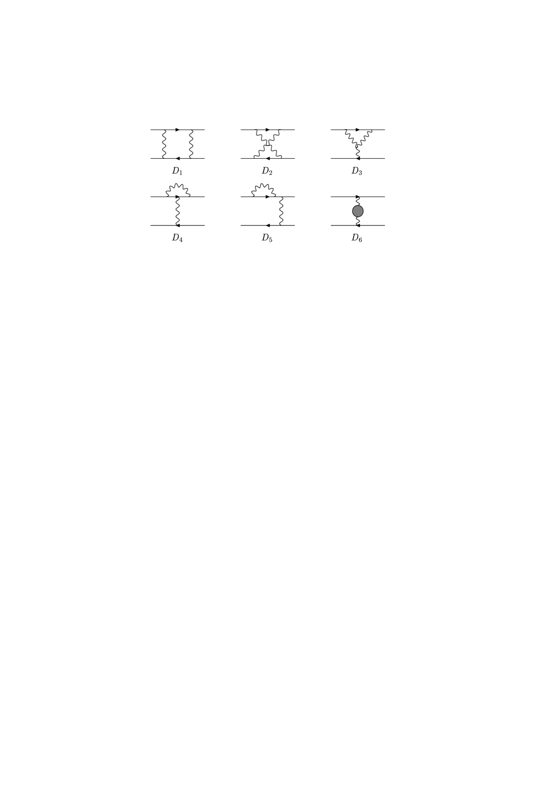
Figure 1: One-loop corrections to the heavy quark potential.

Consider first the one-loop corrections to the potential (see Fig. 1) in dimensional regularisation. In Feynman gauge $D_{3}$ is zero. The colour $C_{F}^{2}$-term cancels in the sum $D_{1}+D_{2}$. $D_{1,2}$ are logarithmically IR divergent. This IR divergence is cancelled by the (logarithmic) scaleless integrals $D_{4,5}$, whose only effect is to convert the IR singularity in $D_{1,2}$ into a UV singularity, which can be absorbed into a renormalisation of $\alpha_{s}$. Hence, we are left with the IR finite parts of (the $C_{A}C_{F}$-part of) $D_{2}$ and $D_{6}$, which yield the well-known one-loop correction to the potential [15, 16]. $D_{6}$ is given in terms of the gluon self-energy at off-shell external momentum $\vec{q}$. For small loop momentum $k$, the integral scales as

$$D_{6}\sim\frac{1}{q^{4}}\int d^{4}k\,\frac{q^{2}}{k^{2}q^{2}}$$ (1)

and gives rise to a contribution of order $\Lambda_{\rm QCD}^{2}/q^{2}$ from the region $k\sim\Lambda_{\rm QCD}$ relative to the tree diagram which scales as $1/q^{2}$. The integral relevant for $D_{2}$ is

$$\int d^{4}k\,\frac{1}{k^{2}(k+q)^{2}(v\cdot k)^{2}},$$ (2)

where $v=(1,\vec{0}\,)$ and $v\cdot q=0$. To find the leading infrared contribution, which is left over after the IR divergence is cancelled as described above, we expand the integrand in $k$ around $k=0$ and around $k+q=0$. The integrals in each term of the expansion depend only on the vector $v$. Hence, in a regularisation scheme that preserves Lorentz invariance all odd terms vanish because $v\cdot q=0$. The long-distance contribution is again of relative order $\Lambda_{\rm QCD}^{2}/q^{2}$. (Note that we are only concerned with IR contributions that are connected with the large-order behaviour of perturbative expansions.)

This argument generalises to an arbitrary diagram. Because $v\cdot q=0$ and because there is no other kinematic invariant linear in $q$, it follows from Lorentz invariance that the leading power correction to the potential in momentum space cannot be $\Lambda_{\rm QCD}/q$, but has to be quadratic:

$$\tilde{V}(q)=-\frac{4\pi C_{F}\alpha_{s}(q)}{q^{2}}\left(1+\frac{\alpha_{s}(q)}{4\pi}\left[\frac{31}{3}-\frac{10n_{f}}{9}\right]+\ldots+\,{\rm const}\times\frac{\Lambda_{\rm QCD}^{2}}{q^{2}}+\ldots\right).$$ (3)

The implication is that the expansion of the potential in the coupling $\alpha_{s}(q)$ diverges as $\sum_{n}r_{n}\alpha_{s}(q)^{n+1}\sim\sum_{n}(-a\beta_{0})^{n}n!n^{b}\alpha_{s}(q)^{n+1}$ with $a=1$ and $\beta_{0}=-(11-2n_{f}/3)/(4\pi)$ the first coefficient of the $\beta$-function. A linear IR power correction would have led to $a=2$ and, hence, a more rapidly divergent perturbative relation. The parameter $b$ remains undetermined by the above analysis, but does not influence the power behaviour.

3. The potential in coordinate space

Consider now the potential in coordinate space, defined by the Fourier transform

$$V(r)=\int\!\frac{d^{3}\vec{q}}{(2\pi)^{3}}\,\,e^{i\vec{q}\cdot\vec{r}}\,\tilde{V}(q).$$ (4)

Note that in the Wilson loop definition of the potential in coordinate space there is a (divergent) constant related to the self-energy of the static sources. This $r$-independent term is usually discarded when one refers to the static potential, and it is also discarded, when $V(r)$ is defined in terms of the Fourier integral above. In what follows the interpretation of this constant plays an important role.

To see that the potential in coordinate space is more sensitive to long distances than the potential in momentum space, it is enough to take the tree approximation to $\tilde{V}(q)$ and to calculate

$$\int\limits_{|\vec{q}\,|<\Lambda_{QCD}}\!\!\!\!\frac{d^{3}\vec{q}}{(2\pi)^{3}}\,\,e^{i\vec{q}\cdot\vec{r}}\,\left(-\frac{4\pi C_{F}\alpha_{s}}{q^{2}}\right)=-\frac{2C_{F}\alpha_{s}}{\pi}\,\Lambda_{\rm QCD}+O(\Lambda_{\rm QCD}^{3}r^{2}).$$ (5)

It follows that the leading power correction is linear in $\Lambda_{\rm QCD}r$:

$$V(r)=-\frac{C_{F}\alpha_{s}(e^{-\gamma_{E}}/r)}{r}\left(1+\frac{\alpha_{s}(e^{-\gamma_{E}}/r)}{4\pi}\left[\frac{31}{3}-\frac{10n_{f}}{9}\right]+\ldots+\,{\rm const}\times\Lambda_{\rm QCD}r+\ldots\right).$$ (6)

($\gamma_{E}$ is Euler’s constant.) The implication is that the expansion of the coordinate space potential in $\alpha_{s}(e^{-\gamma_{E}}r)$ diverges as $\sum_{n}r_{n}\alpha_{s}(e^{-\gamma_{E}}r)^{n+1}\sim\sum_{n}(-a\beta_{0})^{n}n!n^{b}\alpha_{s}(e^{-\gamma_{E}}/r)^{n+1}$ with $a=2$, much faster than the expansion of the potential in momentum space. Note that in absolute terms the IR contribution is a constant of order $\Lambda_{\rm QCD}$.

The rapidly divergent behaviour of the coordinate space potential has been noted in [11] and is discussed in detail in [9, 10]. What we add here is the observation that the linear power correction and, by implication, the rapid divergence originates only from the Fourier transform to coordinate space and is not present in the potential in momentum space. Knowing this we can subtract the leading long-distance contribution and the leading divergent behaviour completely by restricting the Fourier integral to $|\vec{q}\,|>\mu_{f}$ with $\mu_{f}$ a factorisation scale which we make more precise later. The result will be called the ‘subtracted potential’ $V(r,\mu_{f})$. The subtraction terms can be evaluated order by order in $\alpha_{s}$ given $\tilde{V}(q)$ to that order. The relevant calculation will be done in Sect. 5. To be precise, we write

$$V(r,\mu_{f})=V(r)+2\delta m(\mu_{f}),$$ (7)

where

$$\delta m(\mu_{f})=-\frac{1}{2}\int\limits_{|\vec{q}\,|<\mu_{f}}\!\!\!\frac{d^{3}\vec{q}}{(2\pi)^{3}}\,\tilde{V}(q).$$ (8)

To subtract the leading long-distance contribution of order $\Lambda_{\rm QCD}$, it is legitimate to replace $e^{i\vec{q}\cdot\vec{r}}$ by 1 in the Fourier transform and we use this for the definition of the subtraction term. We now define the ‘potential subtracted’ (PS) quark mass parameter as

$$m_{\rm PS}(\mu_{f})=m_{\rm pole}-\delta m(\mu_{f}).$$ (9)

In terms of the subtracted potential and the PS mass the Green function is determined from the Schrödinger-type equation

$$\left[-\frac{\nabla^{2}}{m_{\rm PS}(\mu_{f})}+V(r,\mu_{f})-E\right]G_{C}(\vec{r},E)=\delta^{(3)}(\vec{r}\,),\vspace*{0.1cm}$$ (10)

and it is important that the non-relativistic energy is defined as $E=\sqrt{s}-2m_{\rm PS}(\mu_{f})$, with $s$ the centre-of-mass energy, as compared to the usual definition $\sqrt{s}-2m_{\rm pole}$. The equation above is the conventional Schrödinger equation, but with a ‘residual’ mass term. The subtracted potential $V(r,\mu_{f})$, which contains the residual mass, does not suffer from large loop corrections associated with the leading asymptotic behaviour of its perturbative expansion.

Despite this fact we have not yet gained anything, because the large loop corrections have only been hidden in the contribution $\delta m(\mu_{f})$ to $m_{\rm PS}(\mu_{f})$. The crucial point is this: When $m_{\rm pole}$ is expressed in terms of a ‘short-distance’ mass parameter such as the $\overline{\rm MS}$ mass $m_{\overline{\rm MS}}$ through a perturbative series, this perturbative series also has large loop corrections [12, 13]. The large perturbative corrections absorbed into $\delta m(\mu_{f})$ cancel exactly with large perturbative corrections to the pole mass. The argument is given in the following Section. Hence one can first determine the PS mass from the threshold cross section without encountering large corrections, because of the subtraction in the potential. One can then relate the PS mass to the $\overline{\rm MS}$ mass, again without encountering large corrections related to the asymptotic behaviour of perturbative expansions. In this way, one can, in principle, determine the $\overline{\rm MS}$ mass from threshold cross sections to better accuracy than the pole mass, the use of which is implied by the unsubtracted potential. Conversely, one can begin with $m_{\overline{\rm MS}}$, compute the PS mass and predict the threshold behaviour. The perturbative relation between the PS mass and the $\overline{\rm MS}$ mass is given in Sect. 5.

One may ask why we do not suggest to avoid using the coordinate space potential and to work with the momentum space potential directly. The reason is that the Schrödinger equation for the Coulomb Green function $\tilde{G}_{C}(\vec{p},E)$ in momentum space contains the integration

$$\int\frac{d^{3}k}{(2\pi)^{3}}\,\tilde{V}(\vec{k})\,\tilde{G}_{C}(\vec{p}-\vec{k},E),$$ (11)

which contains exactly the same leading long-distance sensitivity as the Fourier integral (4), because $e^{i\vec{q}\cdot\vec{r}}$ may be replaced by 1 as far as the leading power in $\Lambda_{\rm QCD}r$ is concerned, cf. (8). Hence the problem one encounters with the unsubtracted coordinate space potential enters in momentum space when one solves the Schrödinger equation.

How large can $\mu_{f}$ be? We shall see below that the expansion of $\delta m(\mu_{f})$ is naturally expressed in terms of $\alpha_{s}(\mu_{f})$. Perturbativity hence requires $\mu_{f}>\Lambda_{\rm QCD}$. The scale relevant to the potential is $1/r\sim mv$. Since the subtraction should affect the potential only at distances larger than the physical scale of the process described by the potential we require also $\mu_{f}<mv$. There is another way to arrive at this constraint. If $v=\sqrt{1-4m_{\rm pole}^{2}/s}$ is expanded in terms of $m_{\rm PS}(\mu)$, one generates singular terms (as $v\to 0$) of order $(\delta m(\mu_{f})/(mv^{2}))^{k}$. These terms are small if $\delta m(\mu_{f})$ is small compared to scale $mv^{2}$ of binding energies of a Coulomb system. Counting $\alpha_{s}\sim v$ and using $\delta m(\mu_{f})\sim\mu_{f}\alpha_{s}$, one arrives again at $\mu_{f}<mv$.

4. Cancellation of long-distance contributions with the pole mass

Expressing the pole mass in terms of the $\overline{\rm MS}$ mass and $\delta m(\mu_{f})$ as a series in $\alpha_{s}$, we can write

$$m_{\rm PS}(\mu_{f})=m_{\rm pole}-\delta m(\mu_{f})=M\left[1+\sum_{n=0}r_{n}\alpha_{s}^{n+1}\right]-\mu_{f}\sum_{n=0}s_{n}\alpha_{s}^{n+1},$$ (12)

where $M=m_{\overline{\rm MS}}(m_{\overline{\rm MS}})$. Both series diverge as $r_{n},s_{n}\sim(-a\beta_{0})^{n}n!n^{b}$ with $a=2$. We now show that this behaviour cancels in the difference in (12). Because this divergence arises from long-distance sensitivity of order $\Lambda_{\rm QCD}$ in the Feynman diagrams that contribute to the two series, it is enough to show that the corresponding linear IR behaviour of the Feynman integrands cancels to all orders in perturbation theory in the difference. The remaining long-distance contributions to the difference are of order $\Lambda_{\rm QCD}^{2}/M$ and the corresponding divergent behaviour has only $a=1$. This establishes that the PS mass can be reliably related to the $\overline{\rm MS}$ mass.

Since we are only concerned with infrared behaviour we may work with unrenormalised quantities which differ from $\overline{\rm MS}$ renormalised quantities only by pure UV subtractions. Radiative corrections to the pole mass are given by the self-energy, evaluated at $p^{2}=m_{\rm pole}^{2}$: $\Delta m\equiv m_{\rm pole}-m_{0}=\Sigma_{|\not p=m_{\rm pole}}^{0}$, where $m_{0}$ is the bare mass and $\Sigma^{0}$ the unrenormalised self-energy. Consider the cancellation at the 1-loop order. As long as we are interested only in the leading behaviour at small loop momentum, we can approximate the one-loop contribution to $\Sigma^{0}$ by

$$-iC_{F}g_{s}^{2}\int\!\frac{d^{4}q}{(2\pi)^{4}}\frac{\gamma^{\mu}(\not\!p+\!\not\!q+m_{0})\,\gamma_{\mu}}{((p+q)^{2}-m_{0}^{2})\,q^{2}}\Big{|}_{p^{2}=m_{0}^{2}}\longrightarrow-iC_{F}g_{s}^{2}\int\!\frac{d^{4}q}{(2\pi)^{4}}\frac{1}{(v\cdot q+i\epsilon)\,(q^{2}+i\epsilon)},$$ (13)

setting $p=m_{0}v$. At this order one need not distinguish between $m_{\rm pole}$ and $m_{0}$ in the integrand. Taking the integration over $q_{0}$ in the upper half plane, we obtain

$$-\frac{1}{2}\int\frac{d^{3}\vec{q}}{(2\pi)^{3}}\frac{4\pi C_{F}\alpha_{s}}{-\vec{q}^{\,2}},$$ (14)

which is exactly the leading-order contribution to $\delta m(\mu_{f})$, cf. (8), for small $\vec{q}$. Thus the Feynman integrands of the integrals contributing to $Mr_{0}$ and $\mu_{f}s_{0}$ cancel each other in the infrared region of small $q$. Note that the leading infrared behaviour can be obtained by replacing

$$\frac{1}{v\cdot q+i\epsilon}\longrightarrow-i\pi\,\delta(v\cdot q)$$ (15)

in (13). In other words, the relevant IR behaviour is obtained from setting $q_{0}=0$ first and then from the small-$\vec{q}$ behaviour of the remaining three-dimensional integral.

The denominator of an on-shell heavy quark propagator with momentum $mv+l$ is $v\cdot l+l^{2}/(2m)$. To demonstrate the IR cancellation in higher-loop order, we consider first the static approximation, in which the denominator is simplified to $v\cdot l$ and the gluon coupling $\gamma_{\mu}$ to heavy quarks by $v_{\mu}$. Hence the Feynman rules reduce to those implicit in the definition of the potential. The static approximation implies that we consider all loop momenta small compared to $m$ and take the first term in an expansion in $1/m$. We show that the leading IR contributions of order $\Lambda_{\rm QCD}$ to the pole mass in this approximation cancel exactly with those to the coordinate space potential. At the end of this Section, we address the question of what happens, when one includes further terms in the expansion of the heavy quark propagator in $l$ and the region $l\sim m$, in which the propagator cannot be expanded.

A general self-energy diagram in the static approximation can be written as (see Figure 2a)

$$\int\!\prod_{m=1}^{L}\frac{d^{4}k_{m}}{(2\pi)^{4}}\,S(l_{i})\,\prod_{i=1}^{N}\frac{1}{v\cdot l_{i}+i\epsilon}$$ (16)

where the line momenta $l_{i}$ are linear combinations of the loop momenta $k_{m}$ and $S(l_{i})$ contains no heavy quark propagators. Consider any one-particle irreducible (1PI) subgraph contained entirely in $S$ at fixed, non-zero, external momentum. Such subgraphs are IR finite and at most quadratically IR sensitive. It follows that any subgraph that can give rise to linearly IR sensitive integrals must contain at least one heavy quark propagator with $v\cdot l_{i}\to 0$. Let us call a self-energy diagram (ir-)reducible if it contains (does not contain) a self-energy subgraph.

Figure 2: (a) Structure of an arbitrary self-energy diagram. (b,c) Some 2-loop examples. The double line denotes the static approximation.

Consider irreducible diagrams such as the diagram depicted in Figure 2b first. Irreducible diagrams are IR finite on mass-shell and none of the heavy quark line momenta coincide. The leading IR behaviour is obtained by letting one of the $v\cdot l_{i}=l_{i}^{0}$ go to zero and by neglecting $l_{i}^{0}$ in the other propagators. This can be summarised as the substitution

$$\prod_{i=1}^{N}\frac{1}{v\cdot l_{i}+i\epsilon}\,\longrightarrow\,\sum_{j=1}^{N}\,(-i\pi)\,\delta(v\cdot l_{j})\!\prod_{i=1,\,i\,\not\!=j}^{N}\frac{1}{v\cdot l_{i}+i\epsilon}.$$ (17)

In a term with $\delta(v\cdot l_{j})$ change one loop integration variable to $q=l_{j}(k_{m})$. The delta-function kills the $q_{0}$ integral and sets $q_{0}=0$ in the integrand. One can interpret (17) as cutting the diagram at any heavy quark propagator. This gives rise to $N$ four-point diagrams, to be integrated with $d^{3}\vec{q}/(2\pi)^{3}$, and it is easy to see that the result matches exactly with contributions to $\delta m(\mu_{f})$. For example, the diagram of Figure 2b cancels with the contribution to $\delta m(\mu_{f})$ from $D_{2}+2\cdot D_{4}$ in Figure 1. The signs and $i$’s work out correctly and the factor $1/2$ in (8) comes from the fact that we have $\pi$ in (17) but one factor $1/(2\pi)$ from the four-dimensional integration measure.

One may be concerned about the fact that after setting $q_{0}=0$, the integrals become IR divergent and that hence the leading-order IR approximation (17) may not be sufficient for linearly IR sensitive contributions. The IR divergences are just the IR divergences in individual contributions to the potential mentioned in Sect. 2, which cancel in combinations such as $D_{2}+2\cdot D_{4}$. Moreover, the next term in the small-loop momentum expansion of the integrand is quadratically IR sensitive as shown in Sect. 2, and this is enough to guarantee that (17) is legitimate.

One may also be concerned about the fact that application of (17) does not lead to $D_{2}$ literally, but to an integrand which differs from (2) in that the two factors of $v\cdot k$ have different $i\epsilon$-prescriptions. However, in Sect. 2 we have shown that linearly IR sensitive contributions originate only from the IR behaviour of the Fourier integral. Hence we should consider $q$ small at fixed $k$ or both $q$ and $k$ small simultaneously (but not small $k$ at fixed $q$), in which case the potential pinch singularity is not a problem.

The situation is more complicated for reducible diagrams such as the one in Figure 2c. For reducible diagrams some of the heavy quark line momenta coincide and cutting such a quark line in the sense discussed above leads to one-particle reducible contributions to the potential, i. e. to lower-order contributions to the potential multiplied by on-shell renormalisation of the external legs. ($D_{5}$ in Figure 1 is an example.) Moreover, reducible diagrams are IR divergent when evaluated on-shell, while $\Delta M$ is IR finite. This is related to the fact that $\Delta M$ is not given by $\Sigma_{|\not p=m_{0}}^{0}$ but by $\Sigma_{|\not p=m_{\rm pole}}^{0}$. To make the IR finiteness explicit, the contributions from reducible diagrams to $\Delta M$ should be combined with contributions at the same order in perturbation theory that arise from expanding $\Sigma_{|\not p=m_{\rm pole}}^{0}$ in $\Delta M$:

$$\Sigma_{|\not p=m_{\rm pole}}^{0} = \Sigma_{|\not p=m_{0}}^{0}+\Sigma_{|\not p=m_{0}}^{0}\,\frac{\partial\Sigma^{0}}{\partial\!\!\not\!p}|_{\not p=m_{0}}+\Sigma_{|\not p=m_{0}}^{0}\left(\frac{\partial\Sigma^{0}}{\partial\!\!\not\!p}|_{\not p=m_{0}}\right)^{2}$$ (18)

$$+\,\frac{1}{2}\left(\Sigma_{|\not p=m_{0}}^{0}\right)^{2}\,\frac{\partial^{2}\Sigma^{0}}{\partial\!\!\not\!p^{2}}|_{\not p=m_{0}}+\ldots.$$

This expansion reproduces precisely the combinatorial structure of self-energy subgraphs in reducible diagrams. Combining the various terms on the level of integrands, the resulting integral is IR finite. Moreover, after this cancellation all heavy quark propagators have different momenta and one can again use (17). The ‘cut’ diagrams then cancel again with diagrams to the potential.

Let us illustrate this for the diagram of Figure 2c. According to (18) we combine the diagram with the product of 1-loop contributions to the second term on the right hand side of (18). This gives the following contribution to $\Delta M$:

$$-g_{s}^{4}\int\!\frac{d^{4}k_{1}}{(2\pi)^{4}}\frac{d^{4}k_{2}}{(2\pi)^{4}}\left[\frac{1}{k_{1}^{2}\,k_{2}^{2}\,(v\cdot k_{1})^{2}\,v\cdot(k_{1}+k_{2})}-\frac{1}{k_{1}^{2}\,k_{2}^{2}\,(v\cdot k_{1})^{2}\,v\cdot k_{2}}\right]$$

$$=g_{s}^{4}\int\!\frac{d^{4}k_{1}}{(2\pi)^{4}}\frac{d^{4}k_{2}}{(2\pi)^{4}}\frac{1}{k_{1}^{2}\,k_{2}^{2}\,v\cdot k_{1}\,v\cdot(k_{1}+k_{2})\,v\cdot k_{2}}$$ (19)

$$\longrightarrow\,-\frac{1}{2}\int\!\frac{d^{3}\vec{q}}{(2\pi)^{3}}\,(-i)g_{s}^{4}\int\!\frac{d^{4}k}{(2\pi)^{4}}\left[\frac{-2}{k^{2}\,q^{2}\,(v\cdot k)^{2}}+\frac{1}{k^{2}(k+q)^{2}\,(v\cdot k)^{2}}\right]$$

$$=-\frac{1}{2}\int\!\frac{d^{3}\vec{q}}{(2\pi)^{3}}\,\frac{1}{i}\left[\,4\cdot\frac{1}{2}\cdot D_{5}+D_{1}\right].$$

To arrive at the last two lines we have used (17). Since $1/2\cdot D_{5}$ is the on-shell wave function renormalisation for a single external quark leg times the leading-order potential, we obtain the desired cancellation with IR contributions to the potential. The example and the structure of (18) make it transparent how the IR cancellation for reducible diagrams extends to all orders.

Let us return to the validity of the static approximation. Consider first the contributions to the pole mass from the region of loop momentum where all momenta are small compared to $m$. All heavy quark propagators can be expanded about the static limit. The corrections to the static approximation are suppressed by at least one power of loop momentum divided by $m$. This implies a suppression of long-distance sensitivity by a factor of $\Lambda_{\rm QCD}/m$ relative to the leading term. Since the leading term is already linear in $\Lambda_{\rm QCD}$, we conclude that if the heavy quark line momentum is small, it is sufficient to keep only the leading term in the expansion of the propagator. Consider now the contributions from the region of loop momentum where some loop momenta are of order $m$ and others (at least one) are small compared to $m$. The hard subgraphs with loop momentum of order $m$ reduce to local interactions of form $(l_{i}/m)^{k}$ with respect to the small loop momenta $l_{i}\sim\Lambda_{\rm QCD}$. One obtains contributions suppressed by powers of $\Lambda_{\rm QCD}/m$ unless $k<1$. Hence we need to consider only hard self-energy and vertex subgraphs. The effect of these subgraphs is to renormalise the coefficients of the $\psi^{\dagger}\psi A_{0}$ and $\psi^{\dagger}\partial_{0}\psi$ interaction terms in the non-relativistic effective Lagrangian, from which the potential is derived. In the standard normalisation of the non-relativistic Lagrangian the coefficients of these operators are 1 to all orders in perturbation theory. It follows that the hard subgraphs have no effect on the IR cancellation, or, in other words, they are implicitly taken into account through the coefficient functions of the interaction terms in the non-relativistic Lagrangian which enter the calculation of the Coulomb potential.

5. Relation to the $\overline{\rm MS}$ mass definition

It is straightforward to work out the mass subtraction $\delta m(\mu_{f})$ from known results on the potential in momentum space:

$$\tilde{V}(\vec{q}\,)=-\frac{4\pi C_{F}\alpha_{s}(\vec{q}\,)}{\vec{q}^{\,2}}\left[1+a_{1}\,\frac{\alpha_{s}(\vec{q}\,)}{4\pi}+a_{2}\left(\frac{\alpha_{s}(\vec{q}\,)}{4\pi}\right)^{2}\right]$$ (20)

with $a_{1}$ as in (3) and $a_{2}=634.402-66.3542n_{f}+1.246n_{f}^{2}$ [1]. From the definition (8) one obtains

$$\delta m(\mu_{f}) = \frac{C_{F}\alpha_{s}(\mu)}{\pi}\,\mu_{f}\Bigg{[}1+\frac{\alpha_{s}(\mu)}{4\pi}\left(a_{1}-b_{0}\left(\ln\frac{\mu_{f}^{2}}{\mu^{2}}-2\right)\right)$$

$$+\left(\frac{\alpha_{s}(\mu)}{4\pi}\right)^{2}\Bigg{(}a_{2}-\left\{2a_{1}b_{0}+b_{1}\right\}\left(\ln\frac{\mu_{f}^{2}}{\mu^{2}}-2\right)+b_{0}^{2}\left(\ln^{2}\frac{\mu_{f}^{2}}{\mu^{2}}-4\ln\frac{\mu_{f}^{2}}{\mu^{2}}+8\right)\Bigg{)}\Bigg{]},$$

where $b_{0}=-4\pi\beta_{0}=11-2n_{f}/3$ and $b_{1}=-(4\pi)^{2}\beta_{1}=102-38n_{f}/3$. Note that the logarithms disappear when the coupling is normalised at the scale $\mu_{f}$, which follows from the fact that the potential is physical and independent of $\mu$. At $\mu_{f}=1$-$1.5\,$GeV, a typical scale relevant for bottom quarks, the third-order term already exceeds the second-order term. This is not a point of concern as the series expansion of $\delta m(\mu_{f})$ is expected to behave badly and we are interested only in the combinations $V(r)+2\delta m(\mu_{f})$ and $m_{\rm pole}-\delta m(\mu_{f})$, both of which have better behaved series expansions. The subtracted Coulomb potential $V(r)+2\delta m(\mu_{f})$ at leading order in $\alpha_{s}$ is given by

$$V(r)=-\frac{C_{F}\alpha_{s}(\mu_{r})}{r}\left\{1-\frac{2}{\pi}\,\frac{\alpha_{s}(\mu_{f})}{\alpha_{s}(\mu_{r})}\,\mu_{f}r\right\}$$ (22)

with $\mu_{r}=e^{-\gamma_{E}}/r$. To see the numerical effect of the subtraction, we choose the values $r=1/(20\,\mbox{GeV})$ and $\mu_{f}=3\,$GeV ($n_{f}=5$) as would be appropriate to $t\bar{t}$ production and compare the subtracted and unsubtracted Coulomb potential. The result, including the known higher-order corrections, is

$$V(r,\mu_{f})=-\frac{C_{F}\alpha_{s}(\mu_{r})}{r}\left\{0.86+0.16\,\frac{\alpha_{s}(\mu_{r})}{\pi}+13.64\,\left(\frac{\alpha_{s}(\mu_{r})}{\pi}\right)^{2}+\ldots\right\},$$ (23)

as compared to

$$V(r)=-\frac{C_{F}\alpha_{s}(\mu_{r})}{r}\left\{1+1.19\,\frac{\alpha_{s}(\mu_{r})}{\pi}+32.93\,\left(\frac{\alpha_{s}(\mu_{r})}{\pi}\right)^{2}+\ldots\right\}.$$ (24)

The convergence of the series is improved and the strength of the potential is reduced. For bottom systems one observes a similar effect, although the requirement that $\mu_{f}>\Lambda_{\rm QCD}$ does not allow us to choose $\mu_{f}r$ as small as we would like.

$$\begin{array}[]{c|c|c}\hline\cr\hline\cr\mu_{f}/M&r_{1}^{\rm PS}&r_{2}^{\rm PS}\\ \hline\cr 0&1.33&13.44-1.04n_{f}\\ 1/25&1.28&12.07-0.95n_{f}\\ 1/5&1.07&8.927-0.73n_{f}\\ 1/4&1&8.207-0.68n_{f}\\ 1/3&0.89&7.165-0.61n_{f}\\ \hline\cr\hline\cr\end{array}$$

Table 1: First and second-order (in $\alpha_{s}(M)/\pi$) coefficients in the relation between the PS mass and the $\overline{\rm MS}$ mass (25). For $\mu_{f}=0$ the PS mass coincides with the pole mass.

Since the relation of the pole mass to the $\overline{\rm MS}$ mass is known only to second order [18], we can only make use of $\delta m(\mu_{f})$ to second order to express the potential-subtracted mass $m_{\rm PS}(\mu_{f})=m_{\rm pole}-\delta m(\mu_{f})$ in terms of $M\equiv m_{\overline{\rm MS}}(m_{\overline{\rm MS}})$. The result is

$$m_{\rm PS}(\mu_{f}) = M\,\Bigg{\{}1+\frac{4\alpha_{s}(M)}{3\pi}\left[1-\frac{\mu_{f}}{M}\right]$$ (25)

$$+\left(\frac{\alpha_{s}(M)}{\pi}\right)^{2}\left[K-\frac{\mu_{f}}{3M}\left(a_{1}-b_{0}\left[\ln\frac{\mu_{f}^{2}}{M^{2}}-2\right]\right)\right]+\ldots\Bigg{\}},$$

where $K=13.44-1.04n_{f}$ from [18] and $a_{1}=10.33-1.11n_{f}$. Numerical values for the first and second-order coefficients for various values of $\mu_{f}/M$ are given in Table 1. For small values of $\mu_{f}/M$ as relevant to $t\bar{t}$ production the series is not very different from the series for the pole mass, reflecting the fact that at this order both series still converge well. In absolute terms the difference between the pole and PS mass may still amount to several hundred MeV, which is significant close to threshold. In fact the effect of the subtraction is far from small on the potential even for $t\bar{t}$ production as illustrated by (23) above, because $\mu_{f}$ has to be compared to the scale $m_{t}v/2\sim m_{t}\alpha_{s}/2$ in case of the potential. For ratios of $\mu_{f}/M$ that may be contemplated for bottom quarks near threshold the second-order coefficient in (25) is already considerably smaller than the one in the relation of $m_{\rm pole}$ to $M$ and the convergence of the series expansion is improved. This lends support to the hypothesis that the IR cancellations between $m_{\rm pole}$ and $\delta m(\mu_{f})$ occur not only asymptotically but already at second-order. Eq. (23) and (25) taken together suggest that threshold calculations at NNLO formulated in terms of the subtracted potential and the PS mass exhibit reduced NNLO corrections and that the PS mass can indeed be reliably related to the $\overline{\rm MS}$ mass.

6. Conclusion

In this paper we proposed that perturbative calculations of heavy quark properties near threshold should not use the pole mass but a subtracted mass together with a subtracted potential. This eliminates one source of large corrections in perturbation theory, related to small momentum contributions, although we cannot exclude large corrections due to other reasons. The numerical estimates presented above suggest, however, that the convergence is indeed improved. We emphasise that the potential-subtracted mass is gauge-invariant, because it is derived from the pole mass and an integral over the momentum space potential, both of which are gauge-invariant.

The crucial point is that heavy quark cross sections near threshold are in fact less sensitive to long distances than the quark pole mass parameter. This follows from the observation that the Coulomb potential in momentum space is less sensitive to long distances than the potential in coordinate space and that the large perturbative corrections to the potential in coordinate space cancel to all orders in perturbation theory with those to the pole mass, because of an exact cancellation of the small momentum behaviour of the respective Feynman integrals. That the pole mass is not relevant for physical quantities involving top quarks is quite obvious, because the width of order $1.5\,$GeV provides an intrinsic cut-off for long-distance effects [19]. In particular, the location of the resonance-like peak in the production cross section is not a direct measure of the top quark pole mass despite the fact that top quarks do not hadronise. It is however less obvious that the pole mass is not even relevant for (quasi-) stable quarks near threshold.

Making use of the results of [1] we derived the mass subtraction term to order $\alpha_{s}^{3}$ and the relation between the potential-subtracted (PS) mass and the $\overline{\rm MS}$ mass to order $\alpha_{s}^{2}$. These relations provide the link with other physical quantities involving heavy quarks. In particular, they allow us to determine directly the bottom and top $\overline{\rm MS}$ masses from bottomonium sum rules and the $t\bar{t}$ cross section, thus obviating large NNLO corrections that appear when these quantities are expressed in terms of pole masses [4, 5, 6, 7]. One may hope that this leads to more accurate quark mass determinations than for the pole masses, whose accuracy is limited to order $\Lambda_{\rm QCD}$ by long-distance effects [12, 13] independent of the process utilised to determine them. We will report on these applications in a forthcoming publication.

One cannot use the $\overline{\rm MS}$ masses themselves for threshold problems, because they differ from the pole masses by an amount of order $m\alpha_{s}$. This causes singular terms of order $(\alpha_{s}/v^{2})^{k}$ to appear in perturbative expansions. The all-order resummation of these terms leads one back to the pole mass. It is necessary to introduce a factorisation scale $\mu_{f}$ and to choose a mass definition (the PS mass) that differs from the pole mass by an amount smaller than the typical energies of a Coulomb system, while at the same time not being too sensitive to confinement effects. This leads to a linear dependence on the subtraction scale $\mu_{f}$. The use of a heavy quark mass with a linear factorisation scale dependence has been repeatedly advocated by Bigi et al. (see [13] and the review [20]). In [21] a mass subtraction term $\bar{\Lambda}(\mu_{f})$ (the analogue of our $\delta m(\mu_{f})$) is derived to order $\alpha_{s}^{2}$ from certain integrals over the spectral densities of heavy-light quark currents. This mass subtraction differs from (8) already at order $\alpha_{s}$. This does not imply an inconsistency, since the necessary requirement is only that the long-distance sensitive regions cancel asymptotically in large orders. On the other hand, it seems to us that a subtraction based on the heavy quark Coulomb potential is most natural (and technically simplest) not only for threshold problems involving two heavy quarks, since, as observed in [13], the leading long-distance sensitive contribution to the pole mass is in fact conceptually related to the Coulomb interaction.

Note added: After this paper was completed, we received Ref. [22], which addresses related questions. The authors also note that linear IR sensitivity cancels in $2m_{\rm pole}+V(r)$ and demonstrate this at the 1-loop order.

Acknowledgements. I thank G. Buchalla, A. Signer and V.A. Smirnov for comments on the manuscript and N. Uraltsev for correspondence.

References

- [1] M. Peter, Phys. Rev. Lett. 78 (1997) 602; Nucl. Phys. B501 (1997) 471.
- [2] M. Beneke, A. Signer and V.A. Smirnov, Phys. Rev. Lett. 80 (1998) 2535.
- [3] A. Czarnecki and K. Melnikov, Phys. Rev. Lett. 80 (1998) 2531.
- [4] A.H. Hoang and T. Teubner, UCSD/PTH 98-01 [hep-ph/9801397].
- [5] K. Melnikov and A. Yelkhovsky, BudkerINP-98-7 [hep-ph/9802379].
- [6] A.A. Penin and A.A. Pivovarov, TTP/98-13 [hep-ph/9803363].
- [7] A. Hoang, UCSD/PTH 98-02 [hep-ph/9803454].
- [8] A. Pineda and F.J. Yndurain, UB-ECM-PF-97-34 [hep-ph/9711287]
- [9] M. Jezabek et al., DESY-98-019 [hep-ph/9802373].
- [10] M. Jezabek, M. Peter and Y. Sumino, HD-THEP-98-10 [hep-ph/9803337].
- [11] U. Aglietti and Z. Ligeti, Phys. Lett. B364 (1995) 75.
- [12] M. Beneke and V.M. Braun, Nucl. Phys. B426 (1994) 301; M. Beneke, Phys. Lett. B344 (1995) 341.
- [13] I.I. Bigi, M.A. Shifman, N.G. Uraltsev and A.I. Vainshtein, Phys. Rev. D50 (1994) 2234.
- [14] L. Susskind, Les Houches lectures 1976, in: Weak and electromagnetic interactions at high energies, R. Balian et al. (eds.) (North-Holland, Amsterdam, 1977).
- [15] W. Fischler, Nucl. Phys. B129 (1977) 157.
- [16] T. Appelquist, M. Dine and I.J. Muzinich, Phys. Lett. 69B (1977) 231; Phys. Rev. D17 (1978) 2074.
- [17] M. Beneke and V.A. Smirnov, CERN-97-315, to appear in Nucl. Phys. B [hep-ph/9711391]
- [18] N. Gray, D.J. Broadhurst, W. Grafe and K. Schilcher, Z. Phys. C48 (1990) 673.
- [19] I.I. Bigi et al., Phys. Lett. B181 (1986) 157.
- [20] I.I. Bigi, M.A. Shifman and N.G. Uraltsev, Ann. Rev. Nucl. Part. Sci. 47 (1997) 591.
- [21] A. Czarnecki, K. Melnikov and N. Uraltsev, Phys. Rev. Lett. 80 (1998) 3189.
- [22] A.H. Hoang, M.C. Smith, T. Stelzer and S. Willenbrock, UCSD/PTH 98-13 [hep-ph/9804227].