$B_{s}\rightarrow\gamma\gamma$ decay in the two Higgs doublet model with flavor changing neutral currents


T. M. Aliev ,
Physics Department, Girne American University
Girne , Mersin-10, Turkey

E. O. Iltan
Physics Department, Middle East Technical University
Ankara, Turkey
E-mail address: eiltan@heraklit.physics.metu.edu.tr
Abstract

We calculate the leading logarithmic QCD corrections to the decay $B_{s}\rightarrow\gamma\gamma$ in the two Higgs doublet model with tree level flavor changing currents (model III) including $O_{7}$ type long distance effects. Further, we analyse the dependencies of the branching ratio $Br(B_{s}\rightarrow\gamma\gamma)$ and the ratio of CP-even and CP-odd amplitude squares, $R=|A^{+}|^{2}/|A^{-}|^{2}$, on the charged Higgs mass $m_{H^{\pm}}$ and the selected model III parameters $\xi^{U,D}$ including the leading logarithmic QCD corrections. It is found that to look for charged Higgs effects, the measurement of the branching ratio $Br(B_{s}\rightarrow\gamma\gamma)$ is promising.

1 Introduction

Rare B meson decays constitute one of the most important classes of decays since they are induced by flavor changing neutral currents (FCNC) at loop level in the Standard Model (SM). Therefore they allow us to test the flavor structure of the SM and provide a comprehensive information about the fundamental parameters, such as Cabbibo-Kobayashi-Maskawa (CKM) matrix elements, leptonic decay constants, CP ratio, etc. These decays are also sensitive to the new physics beyond the SM, such as two Higgs Doublet model (2HDM), Minimal Supersymmetric extension of the SM (MSSM) [1], etc.

Among the rare B meson decays, the exclusive $B_{s}\rightarrow\gamma\gamma$ decay has received considerable interest in view of the planned experiments at the upcoming KEK and SLAC-B factories and existing hadronic accelerators, which may measure the branching ratios ($Br$) as low as $10^{-8}$. Since the $B_{s}\rightarrow\gamma\gamma$ decay has two photon system, it is possible to study the CP violating effects [2] and it can be easily detected in the experiments by putting a cut for the energy of final photons [3]. Further, this decay can give information about physics beyond the SM.

The $B_{s}\rightarrow\gamma\gamma$ decay has been studied in the framework of the SM (2HDM) [2],[4]-[5] ([6]) without QCD corrections. It is well-known, that the QCD corrections to the $b\rightarrow s\gamma$ decay are considerably large (see [7] - [10] and references therein). Therefore, one can naturally expect that the situation is the same for the inclusive $b\rightarrow s\gamma\gamma$ decay. Recently, the analysis with the addition of the leading logarithmic (LLog) QCD corrections in the SM [11]-[13], 2HDM [14] and MSSM [15] has been done and the strong sensitivity to QCD corrections was obtained.

The calculations shows that the $Br$ of the decay $B_{s}\rightarrow\gamma\gamma$ is enhanced with the addition of the QCD corrections in the SM. The extension of the Higgs sector (model II in 2HDM) brings extra enhancement to the $Br$. However, the present theoretical results are at the order of ($\sim 10^{-6}$) [14] are far from the experimental upper limit [16]

$\displaystyle Br(B_{s}\rightarrow\gamma\gamma)\leq 1.48\,.10^{-4}\,\,.$ (1)

In the present work, we study this decay in the framework of the two Higgs doublet model with three level flavor changing neutral currents (model III) including perturbative QCD corrections in the LLog approximation, by imposing a method based on heavy quark effective theory for the bound state of the $B_{s}$ meson [11]. Further, we improve our calculations with the inclusion of long-distance effects through the transition $B_{s}\to\phi\gamma\to\gamma\gamma$, which we call $O_{7}$-type, see [11] for details. In the analysis, we use the constraints coming from $\Delta F=2\,(F=K,D,B)$ mixing, the $\rho$ parameter, the ratio Rbe​x​p=Γ​(Zβ†’b​bΒ―)/Γ​(Zβ†’h​a​d​r​o​n​s)(=0.2178Β±0.0011)superscriptsubscript𝑅𝑏𝑒π‘₯𝑝annotatedΞ“β†’π‘π‘Β―π‘Ξ“β†’π‘β„Žπ‘Žπ‘‘π‘Ÿπ‘œπ‘›π‘ absentplus-or-minus0.21780.0011R_{b}^{exp}=\Gamma(Z\rightarrow b\bar{b})/\Gamma(Z\rightarrow hadrons)\,(=0.2178\pm 0.0011) and the CLEO measurement of the decay $B\rightarrow X_{s}\gamma$ [17], for the selected parameters of model III [18], and we get an extreme enhancement for the $Br(B_{s}\rightarrow\gamma\gamma)$. We also predict an upper limit for the model III parameter $\bar{\xi}_{bb}^{D}$ using the present experimental restriction for the $Br$ of the decay $B_{s}\rightarrow\gamma\gamma$, eq.Β (1).

The paper is organized as follows: In section 2, we give the LLog QCD corrected amplitude for the exclusive decay $B_{s}\rightarrow\gamma\gamma$. We further calculate the CP-odd $A^{-}$ and CP-even $A^{+}$ amplitudes in an approach based on heavy quark effective theory, taking the LLog QCD corrections into account. Section 3 is devoted to the analysis of the dependencies of the $Br$ and the ratio $|A^{+}|^{2}/|A^{-}|^{2}$ on the parameters $\mu$ (scale parameter), the Yukawa couplings $\bar{\xi}_{bb}^{D}$, $\bar{\xi}_{tt}^{U}$ and our conclusions. In the appendix , we present the operator basis and the Wilson coefficients responsible for the inclusive $b\rightarrow s\gamma\gamma$ decay in the model III. We also discuss the contributions of the neutral Higgs bosons to the coefficient $C_{7}$ for the decay $b\rightarrow s\gamma$ and the restrictions to the free parameters $\bar{\xi}_{ij}^{D}$, where one of the indices $i$ or $j$ belong to the first or second generation.

2 Leading logarithmic improved short-distance contributions in the model III for the decay $B_{s}\rightarrow\gamma\gamma$

In this section we present the effective Hamiltonian to the exclusive $B_{s}\rightarrow\gamma\gamma$ decay amplitude in the 2HDM with tree level neutral currents (model III). We start with the brief explanation of the model under consideration. The Yukawa interaction in the general case is

$\displaystyle{\cal{L}}_{Y}=\eta^{U}_{ij}\bar{Q}_{iL}\tilde{\phi_{1}}U_{jR}+\eta^{D}_{ij}\bar{Q}_{iL}\phi_{1}D_{jR}+\xi^{U}_{ij}\bar{Q}_{iL}\tilde{\phi_{2}}U_{jR}+\xi^{D}_{ij}\bar{Q}_{iL}\phi_{2}D_{jR}+h.c.\,\,\,,$ (2)

where $L$ and $R$ denote chiral projections $L(R)=1/2(1\mp\gamma_{5})$, $\phi_{i}$ for $i=1,2$, are the two scalar doublets, $\eta^{U,D}_{ij}$ and $\xi^{U,D}_{ij}$ are the matrices of the Yukawa couplings. The choice of $\phi_{1}$ and $\phi_{2}$

$\displaystyle\phi_{1}=\frac{1}{\sqrt{2}}\left[\left(\begin{array}[]{c c}0\\ v+H^{0}\end{array}\right)\;+\left(\begin{array}[]{c c}\sqrt{2}\chi^{+}\\ i\chi^{0}\end{array}\right)\right]\,;\phi_{2}=\frac{1}{\sqrt{2}}\left(\begin{array}[]{c c}\sqrt{2}H^{+}\\ H_{1}+iH_{2}\end{array}\right)\,\,,$ (9)

with the vacuum expectation values,

$\displaystyle<\phi_{1}>=\frac{1}{\sqrt{2}}\left(\begin{array}[]{c c}0\\ v\end{array}\right)\,\,;<\phi_{2}>=0\,\,,$ (12)

permits us to write the Flavor Changing (FC) part of the interaction as

$\displaystyle{\cal{L}}_{Y,FC}=\xi^{U}_{ij}\bar{Q}_{iL}\tilde{\phi_{2}}U_{jR}+\xi^{D}_{ij}\bar{Q}_{iL}\phi_{2}D_{jR}+h.c.\,\,,$ (13)

where the couplings $\xi^{U,D}$ for the FC charged interactions are

$\displaystyle\xi^{U}_{ch}$ $\displaystyle=$ $\displaystyle\xi_{neutral}\,\,V_{CKM}\,\,,$
$\displaystyle\xi^{D}_{ch}$ $\displaystyle=$ $\displaystyle V_{CKM}\,\,\xi_{neutral}\,\,,$ (14)

and $\xi^{U,D}_{neutral}$ 111In all next discussion we denote $\xi^{U,D}_{neutral}$ as $\xi^{U,D}_{N}$. is defined by the expression

$\displaystyle\xi^{U,D}_{N}=(V_{L}^{U,D})^{-1}\xi^{U,D}V_{R}^{U,D}\,\,.$ (15)

Here, the charged couplings appear as a linear combinations of neutral couplings multiplied by $V_{CKM}$ matrix elements.

Now, we would like to discuss the LLog QCD corrections to $b\rightarrow s\gamma\gamma$ decay amplitude in the model III. As it is well known, the effective Hamiltonian method, obtained by integrating out the heavy degrees of freedom, is a powerfull one. In the present case, $t$ quark, $W^{\pm},H^{\pm},H_{1}$, and $H_{2}$ bosons are the heavy degrees of freedom. Here $H^{\pm}$ denote charged, $H_{1}$ and $H_{2}$ denote neutral Higgs bosons. The LLog QCD corrections are done through matching the full theory with the effective low energy theory at the high scale $\mu=m_{W}$ and evaluating the Wilson coefficients from $m_{W}$ down to the lower scale $\mu\sim O(m_{b})$. Note that we choose the higher scale as $\mu=m_{W}$ since the evaluation from the scale $\mu=m_{H^{\pm}}$ to $\mu=m_{W}$ gives negligible contribution to the Wilson coefficients ($\sim 5\%$) since the charged Higgs boson is heavy due to the current theoretical restrictions based on the experimental measurement of $B\rightarrow X_{s}\gamma$ due to the CLEO collaboration [17], for example, $m_{H}^{\pm}\geq 340\,GeV$ [19], $m_{H}^{\pm}\geq 480\,GeV$ [14].

The effective Hamiltonian relevant for our process is

$\displaystyle{\cal{H}}_{eff}=-4\frac{G_{F}}{\sqrt{2}}V_{tb}V^{*}_{ts}\sum_{i}C_{i}(\mu)O_{i}(\mu)\,\,,$ (16)

where the $O_{i}$ are operators given in eqs.Β (31),Β (32) and the $C_{i}$ are Wilson coefficients renormalized at the scale $\mu$. The coefficients $C_{i}$ are calculated perturbatively. The explicit forms of the full-set operators and the corresponding Wilson coefficients are presented in Appendix.

To obtain the decay amplitude for the $B_{s}\rightarrow\gamma\gamma$ decay, we need to sandwich the effective Hamiltonian between the $B_{s}$ and two photon states, i.e. $<B_{s}|{\cal{H}}_{eff}|\gamma\gamma>$. This matrix element can be written in terms of two Lorentz structures [5] - [6], [11]-[13]:

$${\cal A}(B_{s}\rightarrow\gamma\gamma)=A^{+}{\cal F}_{\mu\nu}{\cal F}^{\mu\nu}+iA^{-}{\cal F}_{\mu\nu}\tilde{{\cal F}}^{\mu\nu}\,\,,$$ (17)

where $\tilde{{\cal F}}_{\mu\nu}=\frac{1}{2}\epsilon_{\mu\nu\alpha\beta}{\cal F}^{\alpha\beta}$. Here, the two different operator sets (eqs. (31) and (32)) give contributions to the CP-even $A^{+}$ and CP-odd $A^{-}$ parts. We denote the CP-even (CP-odd) amplitudes due to the first set as $A_{1}^{+}$ ($A_{1}^{-}$) and the second set as $A_{2}^{+}$ ($A_{2}^{-}$). In a HQET inspired approach these amplitudes are:

$\displaystyle A_{1}^{+}$ $\displaystyle=$ $\displaystyle\frac{\alpha_{em}G_{F}}{\sqrt{2}\pi}\frac{f_{B_{s}}}{m_{B_{s}}^{2}}\lambda_{t}\left(\frac{1}{3}\frac{m^{4}_{B_{s}}(m_{b}^{eff}-m_{s}^{eff})}{\bar{\Lambda}_{s}(m_{B_{s}}-\bar{\Lambda}_{s})(m_{b}^{eff}+m_{s}^{eff})}C_{7}^{eff}(\mu)\right.$
$\displaystyle-$ $\displaystyle\left.\frac{4}{9}\frac{m_{B_{s}^{2}}}{m_{b}^{eff}+m_{s}^{eff}}\,[\,(-m_{b}J(m_{b})+m_{s}J(m_{s}))D(\mu)-m_{c}J(m_{c})E(\mu)\,]\,\right),$
$\displaystyle A_{1}^{-}$ $\displaystyle=$ $\displaystyle-\frac{\alpha_{em}G_{F}}{\sqrt{2}\pi}f_{B_{s}}\lambda_{t}\left(\frac{1}{3}\frac{1}{m_{B_{s}}\bar{\Lambda}_{s}(m_{B_{s}}-\bar{\Lambda}_{s})}g_{-}C_{7}^{eff}(\mu)-\sum_{q}Q_{q}^{2}I(m_{q})C_{q}(\mu)\right.$ (18)
$\displaystyle+$ $\displaystyle\left.\frac{1}{9(m_{b}^{eff}+m_{s}^{eff})}[\,(m_{b}\triangle(m_{b})+m_{s}\triangle(m_{s}))D(\mu)+m_{c}\triangle(m_{c})E(\mu)\,]\right)\,\,,$

and

$\displaystyle A_{2}^{+}$ $\displaystyle=$ βˆ’Ξ±e​m​GF2​π​fBsmBs2​λt​(13​mBs4​(mbe​f​fβˆ’mse​f​f)Λ¯s​(mBsβˆ’Ξ›Β―s)​(mbe​f​f+mse​f​f)​C7′⁣e​f​f​(ΞΌ)),subscriptπ›Όπ‘’π‘šsubscript𝐺𝐹2πœ‹subscript𝑓subscript𝐡𝑠superscriptsubscriptπ‘šsubscript𝐡𝑠2subscriptπœ†π‘‘13subscriptsuperscriptπ‘š4subscript𝐡𝑠superscriptsubscriptπ‘šπ‘π‘’π‘“π‘“superscriptsubscriptπ‘šπ‘ π‘’π‘“π‘“subscript¯Λ𝑠subscriptπ‘šsubscript𝐡𝑠subscript¯Λ𝑠superscriptsubscriptπ‘šπ‘π‘’π‘“π‘“superscriptsubscriptπ‘šπ‘ π‘’π‘“π‘“superscriptsubscript𝐢7β€²π‘’π‘“π‘“πœ‡\displaystyle-\frac{\alpha_{em}G_{F}}{\sqrt{2}\pi}\frac{f_{B_{s}}}{m_{B_{s}}^{2}}\lambda_{t}\left(\frac{1}{3}\frac{m^{4}_{B_{s}}(m_{b}^{eff}-m_{s}^{eff})}{\bar{\Lambda}_{s}(m_{B_{s}}-\bar{\Lambda}_{s})(m_{b}^{eff}+m_{s}^{eff})}C_{7}^{\prime eff}(\mu)\right)\,\,,
$\displaystyle A_{2}^{-}$ $\displaystyle=$ $\displaystyle-\frac{\alpha_{em}G_{F}}{\sqrt{2}\pi}f_{B_{s}}\lambda_{t}\left(\frac{1}{3}\frac{1}{m_{B_{s}}\bar{\Lambda}_{s}(m_{B_{s}}-\bar{\Lambda}_{s})}g_{-}C_{7}^{\prime eff}(\mu)\right)\,\,,$ (19)

where $Q_{q}=\frac{2}{3}$ for $q=u,c$ and $Q_{q}=-\frac{1}{3}$ for q=d,s,bπ‘žπ‘‘π‘ π‘q=d,s,b. Here, we have used the unitarity of the CKM-matrix $\sum_{i=u,c,t}V_{is}^{*}V_{ib}=0$ and have neglected the contribution due to $V_{us}^{*}V_{ub}\ll V_{ts}^{*}V_{tb}\equiv\lambda_{t}$. The function $g_{-}$ is defined as [11]:

gβˆ’=mBs​(mbe​f​f+mse​f​f)2+Λ¯s​(mBs2βˆ’(mbe​f​f+mse​f​f)2).subscript𝑔subscriptπ‘šsubscript𝐡𝑠superscriptsuperscriptsubscriptπ‘šπ‘π‘’π‘“π‘“superscriptsubscriptπ‘šπ‘ π‘’π‘“π‘“2subscript¯Λ𝑠subscriptsuperscriptπ‘š2subscript𝐡𝑠superscriptsuperscriptsubscriptπ‘šπ‘π‘’π‘“π‘“superscriptsubscriptπ‘šπ‘ π‘’π‘“π‘“2\displaystyle g_{-}=m_{B_{s}}(m_{b}^{eff}+m_{s}^{eff})^{2}+\bar{\Lambda}_{s}(m^{2}_{B_{s}}-(m_{b}^{eff}+m_{s}^{eff})^{2})\,\,. (20)

The parameter $\bar{\Lambda}_{s}$ enters eq.Β (18) and Β (19) through the bound state kinematics [11]. Now, we would like explain the approach we follow to be clear how to get the amplitudes ( eqs. Β (18) and Β (19)). The momentum of the $\bar{b}-$quark inside the $B_{s}$ meson can be written as $p=m_{b}v+k$, where $k$ is the residual momentum and $v$ is the 4-velocity defined by $v=p_{B}/m_{B_{s}}$. Here $p_{B}$ is the 4-momentum of the meson $B_{s}$. In the matrix elements we need to evaluate $p.k_{i}$ and $p^{\prime}.k_{i}$, $i=1,2$, where $k_{i}$, $p^{\prime}$ are the momenta of the outgoing photon and $s$ -quark respectively. We average the residual momentum of the $\bar{b}$ quark as [20]

$\displaystyle<k_{\mu}>=-\frac{1}{2m_{b}}(\lambda_{1}+3\lambda_{2})v_{\mu}\,\,,$
$\displaystyle<k_{\mu}k_{\nu}>=\frac{\lambda_{1}}{3}(g_{\mu\nu}-v_{\mu}v_{\nu})\,\,,$ (21)

where $\lambda_{1}$, $\lambda_{2}$ are matrix elements from heavy quark expansion. $\lambda_{2}\,(=0.12\,GeV)$ can be determined from the $B^{*}_{(s)}-B_{(s)}$ mass splitting.

Finally we have

$\displaystyle p.k_{i}$ $\displaystyle=$ $\displaystyle\frac{m_{B_{s}}}{2}(m_{B_{s}}-\bar{\Lambda}_{s})\,\,,$
$\displaystyle p^{\prime}.k_{i}$ $\displaystyle=$ $\displaystyle-\frac{m_{B_{s}}}{2}\bar{\Lambda}_{s}\,\,,$
$\displaystyle(m_{b}^{eff})^{2}$ $\displaystyle=$ $\displaystyle p^{2}=m_{b}^{2}-3\lambda_{2}\,\,,$
(mse​f​f)2superscriptsuperscriptsubscriptπ‘šπ‘ π‘’π‘“π‘“2\displaystyle(m_{s}^{eff})^{2} $\displaystyle=$ p′⁣2=(mse​f​f)2βˆ’mBs2+2​mBs​Λ¯s.superscript𝑝′2superscriptsuperscriptsubscriptπ‘šπ‘ π‘’π‘“π‘“2superscriptsubscriptπ‘šsubscript𝐡𝑠22subscriptπ‘šsubscript𝐡𝑠subscript¯Λ𝑠\displaystyle p^{\prime 2}=(m_{s}^{eff})^{2}-m_{B_{s}}^{2}+2m_{B_{s}}\bar{\Lambda}_{s}\,\,. (22)

Here, we use the definitions $p_{B}=p-p^{\prime}$, $p_{B}.k_{i}=\frac{m_{B_{s}}^{2}}{2}$, $v.k_{i}=\frac{m_{B_{s}}}{2}$ and the HQET relation [20]

$\displaystyle m_{B_{s}}=m_{b}+\bar{\Lambda}_{s}-\frac{1}{2m_{b}}(\lambda_{1}+3\lambda_{2})\,\,,$ (23)

In eq. (22), $m_{b}^{eff}$ and mse​f​fsuperscriptsubscriptπ‘šπ‘ π‘’π‘“π‘“m_{s}^{eff} are the effective masses of the quarks in the $B_{s}$ meson bound state [11] and the parameter $\bar{\Lambda}_{s}$ can be defined as Λ¯s=Λ¯+Δ​msubscriptΒ―Ξ›π‘ Β―Ξ›Ξ”π‘š\bar{\Lambda}_{s}=\bar{\Lambda}+\Delta m. $\bar{\Lambda}$ together with $\lambda_{1}$ can be extracted from data on semileptonic $B^{\pm}\,,B_{0}$ decays [21] and the measured mass difference $\Delta m=m_{B_{s}}-m_{B}=90\,MeV$ [22]. Using eq. (23), we correlate the parameters $\bar{\Lambda}_{s}$ and $m_{b}$ and $\bar{\Lambda}$ and $\lambda_{1}$ (Table (Β 1)).

After this brief explanation of the HQET inspired approach we follow, we continue with the LLog QCD-corrected Wilson coefficients $C_{1\dots 10}(\mu)$ [11] - [13] which enter the amplitudes in the combinations

$\displaystyle C_{u}(\mu)$ $\displaystyle=$ $\displaystyle C_{d}(\mu)=(C_{3}(\mu)-C_{5}(\mu))N_{c}+C_{4}(\mu)-C_{6}(\mu)\,\,,$
$\displaystyle C_{c}(\mu)$ $\displaystyle=$ $\displaystyle(C_{1}(\mu)+C_{3}(\mu)-C_{5}(\mu))N_{c}+C_{2}(\mu)+C_{4}(\mu)-C_{6}(\mu)\,\,,$
Cs​(ΞΌ)subscriptπΆπ‘ πœ‡\displaystyle C_{s}(\mu) $\displaystyle=$ $\displaystyle C_{b}(\mu)=(C_{3}(\mu)+C_{4}(\mu))(N_{c}+1)-N_{c}C_{5}(\mu)-C_{6}(\mu)\,\,,$
$\displaystyle D(\mu)$ $\displaystyle=$ $\displaystyle C_{5}(\mu)+C_{6}(\mu)N_{c}\,\,,$
$\displaystyle E(\mu)$ $\displaystyle=$ $\displaystyle C_{10}(\mu)+C_{9}(\mu)N_{c}$ (24)

where $N_{c}$ is the number of colours ($N_{c}=3$ for QCD).

The effective coefficients $C_{7}^{eff}(\mu)$ and $C_{7}^{\prime eff}(\mu)$ are defined in the NDR scheme, which we use here, as [18]

$\displaystyle C_{7}^{eff}(\mu)$ $\displaystyle=$ $\displaystyle C_{7}^{2HDM}(\mu)+Q_{d}\,(C_{5}^{2HDM}(\mu)+N_{c}\,C_{6}^{2HDM}(\mu))\,\,,$
$\displaystyle+$ $\displaystyle Q_{u}\,(\frac{m_{c}}{m_{b}}\,C_{10}^{2HDM}(\mu)+N_{c}\,\frac{m_{c}}{m_{b}}\,C_{9}^{2HDM}(\mu))\,\,,$
$\displaystyle C^{\prime eff}_{7}(\mu)$ $\displaystyle=$ $\displaystyle C^{\prime 2HDM}_{7}(\mu)+Q_{d}\,(C^{\prime 2HDM}_{5}(\mu)+N_{c}\,C^{\prime 2HDM}_{6}(\mu))$ (25)
$\displaystyle+$ $\displaystyle Q_{u}(\frac{m_{c}}{m_{b}}\,C_{10}^{\prime 2HDM}(\mu)+N_{c}\,\frac{m_{c}}{m_{b}}\,C_{9}^{\prime 2HDM}(\mu))\,\,.$

The functions $I(m_{q}),\,J(m_{q})$ and $\triangle(m_{q})$ come from the irreducible diagrams with an internal $q$ type quark propagating and are defined as

$\displaystyle I(m_{q})$ $\displaystyle=$ $\displaystyle 1+\frac{m_{q}^{2}}{m_{B_{s}}^{2}}\triangle(m_{q})\,\,,$
$\displaystyle J(m_{q})$ $\displaystyle=$ $\displaystyle 1-\frac{m_{B_{s}}^{2}-4m_{q}^{2}}{4m_{B_{s}}^{2}}\triangle(m_{q})\,\,,$
$\displaystyle\triangle(m_{q})$ $\displaystyle=$ $\displaystyle\left(\ln(\frac{m_{B_{s}}+\sqrt{m_{B_{s}}^{2}-4m_{q}^{2}}}{m_{B_{s}}-\sqrt{m_{B_{s}}^{2}-4m_{q}^{2}}})-i\pi\right)^{2}\,\,{\mbox{for}}\,\,\frac{m^{2}_{B_{s}}}{4m_{q}^{2}}\geq 1,$
$\displaystyle\triangle(m_{q})$ $\displaystyle=$ βˆ’(2​arctan⁑(4​mq2βˆ’mBs2mBs)βˆ’Ο€)2​for​mBs24​mq2< 1.superscript24superscriptsubscriptπ‘šπ‘ž2superscriptsubscriptπ‘šsubscript𝐡𝑠2subscriptπ‘šsubscriptπ΅π‘ πœ‹2forsubscriptsuperscriptπ‘š2subscript𝐡𝑠4superscriptsubscriptπ‘šπ‘ž21\displaystyle-\left(2\arctan(\frac{\sqrt{4m_{q}^{2}-m_{B_{s}}^{2}}}{m_{B_{s}}})-\pi\right)^{2}\,\,{\mbox{for}}\,\,\frac{m^{2}_{B_{s}}}{4m_{q}^{2}}<\ 1. (26)

Finally the CP-even $A^{-}$ and CP-odd $A^{+}$ amplitudes can be written as

$\displaystyle A^{+}$ $\displaystyle=$ $\displaystyle A_{1}^{+}+A_{2}^{+}\,\,,$
$\displaystyle A^{-}$ $\displaystyle=$ $\displaystyle A_{1}^{-}+A_{2}^{-}\,\,,$ (27)

where the amplitudes $A_{1}^{\pm}$ and $A_{2}^{\pm}$ are given in eqs.  (18) and  (19) respectively.

In our numerical analysis we used the input values given in TableΒ (1).

Parameter Value
$m_{c}$ $1.4$ (GeV)
$m_{b}$ $4.8$ (GeV)
$\alpha_{em}^{-1}$ 129
$\lambda_{t}$ 0.04
$\Gamma_{tot}(B_{s})$ $4.09\cdot 10^{-13}$ (GeV)
$f_{B_{s}}$ $0.2$ (GeV)
$m_{B_{s}}$ $5.369$ (GeV)
$m_{t}$ $175$ (GeV)
$m_{W}$ $80.26$ (GeV)
$m_{Z}$ $91.19$ (GeV)
$\Lambda^{(5)}_{QCD}$ $0.214$ (GeV)
$\alpha_{s}(m_{Z})$ $0.117$
$\lambda_{2}$ $0.12$ $(\mbox{GeV}^{2})$
$\lambda_{1}$ $-0.29$ $(\mbox{GeV}^{2})$
$\bar{\Lambda}_{s}$ $590$ $(\mbox{MeV})$
$\bar{\Lambda}$ $500$ $(\mbox{MeV})$
Table 1: Values of the input parameters used in the numerical calculations unless otherwise specified.

3 Discussion

Before we present our numerical results, we would like to discuss briefly the free parameters of the model under consideration, i.e. model III. This model induces many free parameters, such as $\xi_{ij}^{U,D}$ where i,j are flavor indices. To obtain qualitative results, we should restrict them using the experimental measurements. The explicit expressions of $C_{7}^{h_{0}}$ and $C_{7}^{A_{0}}$ (eq. (34)) show that the the neutral Higgs bosons can give a large contribution to the coefficient $C_{7}$ which can be in contradiction with the CLEO data [17],

$\displaystyle Br(B\rightarrow X_{s}\gamma)=(2.32\pm 0.07\pm 0.35)\,10^{-4}\,\,.$ (28)

Such potentially dangerous terms are removed with the assumption that the couplings ΞΎΒ―N,i​sDsubscriptsuperscriptΒ―πœ‰π·π‘π‘–π‘ \bar{\xi}^{D}_{N,is}($i=d,s,b)$ and $\bar{\xi}^{D}_{N,db}$ are negligible to be able to reach the conditions ΞΎΒ―N,b​bD​ξ¯N,i​sD<<1much-less-thansubscriptsuperscriptΒ―πœ‰π·π‘π‘π‘subscriptsuperscriptΒ―πœ‰π·π‘π‘–π‘ 1\bar{\xi}^{D}_{N,bb}\,\bar{\xi}^{D}_{N,is}<<1 and ΞΎΒ―N,d​bD​ξ¯N,d​sD<<1much-less-thansubscriptsuperscriptΒ―πœ‰π·π‘π‘‘π‘subscriptsuperscriptΒ―πœ‰π·π‘π‘‘π‘ 1\bar{\xi}^{D}_{N,db}\,\bar{\xi}^{D}_{N,ds}<<1. Further, we use the constraints [18] coming from the ratio Rbe​x​p=Γ​(Zβ†’b​bΒ―)/Γ​(Zβ†’h​a​d​r​o​n​s)superscriptsubscript𝑅𝑏𝑒π‘₯π‘Ξ“β†’π‘π‘Β―π‘Ξ“β†’π‘β„Žπ‘Žπ‘‘π‘Ÿπ‘œπ‘›π‘ R_{b}^{exp}=\Gamma(Z\rightarrow b\bar{b})/\Gamma(Z\rightarrow hadrons), namely $\xi^{D}_{Nbb}>\frac{60m_{b}}{v}$, the restrictions due to the $\Delta F=2$ mixing, the $\rho$ parameter [23], and the measurement by CLEO collaboration. The analysis of the mentioned processes and the discussion given above, leads to choose $\bar{\xi}_{Ntc}<<\bar{\xi}^{U}_{Ntt},\bar{\xi}^{D}_{Nbb}$ and $\bar{\xi}^{D}_{Nib}\sim 0\,,\bar{\xi}^{D}_{Nij}\sim 0$, where the indices $i,j$ denote d and s quarks .

After these preliminary remarks, let us start with our numerical analysis. In this section we study the dependencies of the B​rπ΅π‘ŸBr and the ratio R=|A+|2/|Aβˆ’|2𝑅superscriptsuperscript𝐴2superscriptsuperscript𝐴2R=|A^{+}|^{2}/|A^{-}|^{2} on the selected parameters of the model III (ΞΎΒ―N​t​tUsubscriptsuperscriptΒ―πœ‰π‘ˆπ‘π‘‘π‘‘\bar{\xi}^{U}_{Ntt}, ΞΎΒ―N​b​bDsubscriptsuperscriptΒ―πœ‰π·π‘π‘π‘\bar{\xi}^{D}_{Nbb} and mHΒ±subscriptπ‘šsuperscript𝐻plus-or-minusm_{H^{\pm}}) and the QCD scale ΞΌπœ‡\mu. In figs.Β 1 and 2 (Β 3 and Β 4) we plot the B​rπ΅π‘ŸBr of the decay Bs→γ​γ→subscript𝐡𝑠𝛾𝛾B_{s}\rightarrow\gamma\gamma with respect to the charged Higgs mass mHΒ±subscriptπ‘šsuperscript𝐻plus-or-minusm_{H^{\pm}} for the fixed value of ΞΎΒ―N,b​bD=60​mbsuperscriptsubscriptΒ―πœ‰π‘π‘π‘π·60subscriptπ‘šπ‘\bar{\xi}_{N,bb}^{D}=60\,m_{b} (ΞΎΒ―N,b​bD=90​mbsuperscriptsubscriptΒ―πœ‰π‘π‘π‘π·90subscriptπ‘šπ‘\bar{\xi}_{N,bb}^{D}=90\,m_{b}) at three different ΞΌπœ‡\mu scales (ΞΌ=2.5,5,mW)GeV\mu=2.5\,,5\,,m_{W}\,)GeV. Fig.Β 1 (3) represents the case where the ratio |rt​b|=|ΞΎΒ―N,t​tUΞΎΒ―N,b​bD|<<1subscriptπ‘Ÿπ‘‘π‘superscriptsubscriptΒ―πœ‰π‘π‘‘π‘‘π‘ˆsuperscriptsubscriptΒ―πœ‰π‘π‘π‘π·much-less-than1|r_{tb}|=|\frac{\bar{\xi}_{N,tt}^{U}}{\bar{\xi}_{N,bb}^{D}}|<<1 and shows that the B​rπ΅π‘ŸBr obtained in the model III almost coincides with the one calculated in the SM. The suppression of the contribution coming from the charged Higgs boson can be seen from eqs.Β (36) and 18 with the choice |rt​b|<<1much-less-thansubscriptπ‘Ÿπ‘‘π‘1|r_{tb}|<<1. However in fig.Β 2 (4), the B​rπ΅π‘ŸBr is presented for the case rt​b>>1much-greater-thansubscriptπ‘Ÿπ‘‘π‘1r_{tb}>>1. It is seen that there is an extreme enhancement of the B​rπ΅π‘ŸBr, especially for the small values of mHΒ±subscriptπ‘šsuperscript𝐻plus-or-minusm_{H^{\pm}}. Note that this is similar to the result coming from the choice of t​a​n​β<1π‘‘π‘Žπ‘›π›½1tan\beta<1 in the model II [14]. In figs.Β 5 Β (6) we present ΞΎΒ―N,b​bDsuperscriptsubscriptΒ―πœ‰π‘π‘π‘π·\bar{\xi}_{N,bb}^{D} dependence of the B​rπ΅π‘ŸBr at the fixed value of mHΒ±=500​G​e​Vsubscriptπ‘šsuperscript𝐻plus-or-minus500𝐺𝑒𝑉m_{H^{\pm}}=500\,GeV for |rt​b|<<1much-less-thansubscriptπ‘Ÿπ‘‘π‘1|r_{tb}|<<1 (rt​b>>1much-greater-thansubscriptπ‘Ÿπ‘‘π‘1r_{tb}>>1). In the region |rt​b|<<1much-less-thansubscriptπ‘Ÿπ‘‘π‘1|r_{tb}|<<1, the B​rπ΅π‘ŸBr is nonsensitive to the coupling ΞΎΒ―N,b​bDsuperscriptsubscriptΒ―πœ‰π‘π‘π‘π·\bar{\xi}_{N,bb}^{D} and almost coincides with the SM value, however for rt​b>>1much-greater-thansubscriptπ‘Ÿπ‘‘π‘1r_{tb}>>1, it increases with the increasing ΞΎΒ―N,b​bDsuperscriptsubscriptΒ―πœ‰π‘π‘π‘π·\bar{\xi}_{N,bb}^{D}. Note that the B​rπ΅π‘ŸBr is sensitive to the scale ΞΌπœ‡\mu. For |rt​b|<<1much-less-thansubscriptπ‘Ÿπ‘‘π‘1|r_{tb}|<<1, it increases with decreasing ΞΌπœ‡\mu (figs.Β 1, 3 and 5 ) similar to the model II [14]. For rt​b>>1much-greater-thansubscriptπ‘Ÿπ‘‘π‘1r_{tb}>>1, decreasing the scale ΞΌπœ‡\mu causes the B​rπ΅π‘ŸBr to decrease. (figs.Β 2, 4 and 6).

At this stage we would like to estimate the upper limit of $\bar{\xi}_{N,bb}^{D}$ for $r_{tb}>>1$ by using the present experimental result $Br(B_{s}\rightarrow\gamma\gamma)\leq 1.48\cdot 10^{-4}$. By choosing the lower limit for the mass $m_{H^{\pm}}\sim 480\,GeV$ [14] at the scale $\mu=2.5\,GeV$, we get $\bar{\xi}_{N,bb}^{D}<90\,m_{b}$. It is interesting to note that the increasing value of $m_{H^{\pm}}$ makes the restriction region for $\bar{\xi}_{N,bb}^{D}$ smaller.

Since the two photon system can be in a CP-even and CP-odd state, $B_{s}\rightarrow\gamma\gamma$ decay allows us to study CP violating effects. In the rest frame of the $B_{s}$ meson, the $CP=-1$ amplitude $A^{-}$ is proportional to the perpendicular spin polarization $\vec{\epsilon_{1}}\times\vec{\epsilon_{2}}$, and the $CP=1$ amplitude $A^{+}$ is proportional to the parallel spin polarization $\vec{\epsilon_{1}}.\vec{\epsilon_{2}}$. The ratio $R$ is informative to search for CP violating effects in $B_{s}\rightarrow\gamma\gamma$ decays and it has been studied before in the literature in the framework of the 2HDM without [6] and with [14] QCD corrections.

Now, we present the dependence of the ratio $R=|A^{+}|^{2}/|A^{-}|^{2}$ on the selected parameters of model III, displayed in a series of figures (Β 7 - 11). In figs.Β 7 and Β 8 we plot the dependence of $R$ on $m_{H^{\pm}}$ for fixed $\bar{\xi}_{N,bb}^{D}=60\,m_{b}$ and three different $\mu$ scales, $(2.5\,,5\,,m_{W})\,\,GeV$. The $R$ ratio is almost nonsensitive to $m_{H^{\pm}}$ for $|r_{tb}|<<1$ (fig.Β 7). However, it is enhanced with the increasing value of $m_{H^{\pm}}$ ($m_{H^{\pm}}\leq 1000\,GeV$) for $r_{tb}>>1$ (fig.Β 8). Decreasing the scale $\mu$ weakens the dependence of the ratio $R$ on $m_{{H}^{\pm}}$ and the contribution of the charged Higgs bosons to the $R$ ratio becomes small similar to the model II [14]. Further, it becomes less dependent to $m_{H^{\pm}}$ with increasing $\bar{\xi}_{N,bb}^{D}$ (fig Β 8, Β 9).

Fig.Β 10 and 11 show the dependence of $R$ on $\bar{\xi}_{N,bb}^{D}$ for fixed $m_{{H}^{\pm}}=500\,\,GeV$. Like the previous case, $R$ dependence to the coupling $\bar{\xi}_{N,bb}^{D}$ is extremely weak for $|r_{tb}|<<1$. (fig.Β 10). For $r_{tb}>>1$ the ratio $R$ increases with decreasing $\bar{\xi}_{N,bb}^{D}$ (fig Β 11). Note that, this ratio can exceed one unlike the SM case. The same situation appears in model II also [14].

The ratio R𝑅R is quite sensitive to QCD corrections and it is enhanced with decreasing scale ΞΌπœ‡\mu for the SM and |rt​b|<<1much-less-thansubscriptπ‘Ÿπ‘‘π‘1|r_{tb}|<<1 (figs.Β 7, 10). However, this ratio decreases for rt​b>>1much-greater-thansubscriptπ‘Ÿπ‘‘π‘1r_{tb}>>1 (figs.Β 8,Β 9, Β 11). We observe, that the smaller the value of mHΒ±subscriptπ‘šsuperscript𝐻plus-or-minusm_{H^{\pm}} (the larger the value of ΞΎΒ―N,b​bDsuperscriptsubscriptΒ―πœ‰π‘π‘π‘π·\bar{\xi}_{N,bb}^{D}), the less dependent is the ratio on ΞΌπœ‡\mu. This strong ΞΌπœ‡\mu dependence makes the analysis of the model III parameters mHΒ±subscriptπ‘šsuperscript𝐻plus-or-minusm_{H^{\pm}} and ΞΎΒ―U,DsuperscriptΒ―πœ‰π‘ˆπ·\bar{\xi}^{U,D} for the given experimental value of the ratio R𝑅R to be difficult, especially for the case |rt​b|<<1much-less-thansubscriptπ‘Ÿπ‘‘π‘1|r_{tb}|<<1. However, we believe, that the strong ΞΌπœ‡\mu dependence will be reduced with the addition the of next to leading order (NLO) calculation. This requires a computation of finite parts of many two loop diagrams, and divergent part of three-loop diagrams. This lies beyond the scope of the present work and it has to be done to reduce the uncertainity coming from the scale ΞΌπœ‡\mu. Fortunately, the choice of ΞΌ=mb/2πœ‡subscriptπ‘šπ‘2\mu=m_{b}/2 in the LLog approximation reproduces effectively the NLO result for the bβ†’s​γ→𝑏𝑠𝛾b\rightarrow s\gamma decay and one can suggest that it may also work for the bβ†’s​γ​γ→𝑏𝑠𝛾𝛾b\rightarrow s\gamma\gamma decay. In any case, the analysis on the model III parameters will be more reliable after NLO calculations are done.

We complete this section by taking the $O_{7}$ type long distance effects ($LD_{O_{7}}$) for both the $Br$ and the ratio $R$ into account. The $LD_{O_{7}}$ contribution to the CP-odd $A^{-}$ and CP-even $A^{+}$ amplitudes has been calculated with the help of the Vector Meson Dominance model (VMD) [11] and it was shown, that the influence on the amplitudes was destructive. With the addition of the $LD_{O_{7}}$ effects, the amplitudes entering the $Br$ and $R$ ratio are now given as

$\displaystyle A^{+}$ $\displaystyle=$ $\displaystyle A^{+}_{SD}+A^{+}_{LD_{O_{7}}}\,\,,$
$\displaystyle A^{-}$ $\displaystyle=$ $\displaystyle A^{-}_{SD}+A^{-}_{LD_{O_{7}}}\,\,,$ (29)

where $A^{\pm}_{SD}$ are the short distance amplitudes we took into account in the previous sections (eq.(27)). The $LD_{O_{7}}$ amplitudes $A^{\pm}_{LD_{O_{7}}}$ are defined as [11]

$\displaystyle A^{+}_{LD_{O_{7}}}$ $\displaystyle=$ $\displaystyle-\sqrt{2}\frac{\alpha_{em}G_{F}}{\pi}\bar{F_{1}}(0)f_{\phi}(0)\lambda_{t}\frac{m_{b}(m_{B_{s}}^{2}-m_{\phi}^{2})}{3m_{\phi}m_{B_{s}}^{2}}C_{7}^{eff}(\mu)\,\,,$
$\displaystyle A^{-}_{LD_{O_{7}}}$ $\displaystyle=$ $\displaystyle\sqrt{2}\frac{\alpha_{em}G_{F}}{\pi}\bar{F_{1}}(0)f_{\phi}(0)\lambda_{t}\frac{m_{b}}{3m_{\phi}}C_{7}^{eff}(\mu)\,\,,$ (30)

where $f_{\phi}(0)=0.18\,\,GeV$ is the decay constant of $\phi$ meson at zero momentum, $\bar{F}_{1}(0)$ is the extrapolated $B_{s}\rightarrow\phi$ form factor (for details see [11]). Note that we neglect the contribution of operator $O^{\prime}_{7}$ in eq.(Β 30) since the coefficient $C_{7}^{\prime eff}(\mu)$ is negligible compared to the coefficient $C_{7}^{eff}(\mu)$ (see the discussion given in appendix).

In figs. (Β 12 -Β 17 ) we present the mHΒ±subscriptπ‘šsuperscript𝐻plus-or-minusm_{H^{\pm}} and ΞΎΒ―N,b​bDsuperscriptsubscriptΒ―πœ‰π‘π‘π‘π·\bar{\xi}_{N,bb}^{D} dependencies of the B​rπ΅π‘ŸBr and the ratio R𝑅R with the addition of L​DO7𝐿subscript𝐷subscript𝑂7LD_{O_{7}} effects. Here we use FΒ―1​(0)=0.16subscript¯𝐹100.16\bar{F}_{1}(0)=0.16 [11]. The B​rπ΅π‘ŸBr decreases with the addition of L​DO7𝐿subscript𝐷subscript𝑂7LD_{O_{7}} effects, since the effect is destructive. The ΞΌπœ‡\mu scale uncertanity of the B​rπ΅π‘ŸBr is smaller compared to the case where LD effect is not included.

It can be shown, that the value of the ratio $R$ also decreases with the addition of $LD_{O_{7}}$ effects for the SM case. (figs. Β 15 - 17). However, while $m_{H^{\pm}}$ is increasing or $\bar{\xi}_{N,bb}^{D}$ is decreasing, the effect of the $LD_{O_{7}}$ contribution on the ratio $R$ is increasing for $r_{tb}>>1$ (figs.Β 16, Β 17).

There are still non-perturbative effects which can come from the formation of $c\bar{c}$ bound states. However these states are far off-shell and do not give significant contribution to the decay rate [13]. For example the chain process $B_{s}\rightarrow\phi\psi\rightarrow\phi\gamma\rightarrow\gamma\gamma$ is estimated and it is found to be at most $1\%$ of the branching ratio $Br(B_{s}\rightarrow\gamma\gamma)_{SD+LD_{O_{7}}}$ [24]

Besides the strong $\mu$ dependence there is another uncertainity coming from the choice of bound state parameters $m_{b}^{eff}$ and $\bar{\Lambda}_{s}$. It follows that the larger $m_{b}^{eff}$ (smaller $\bar{\Lambda}_{s}$), the larger $Br$ and $R$ ratio. Here the enhacement of the $Br$ is caused by the $\frac{1}{\bar{\Lambda}_{s}}$ dependence in amplitudes.

In conclusion, we analyse the selected model III parameters ( $\bar{\xi}_{N,bb}^{D}$, $\bar{\xi}_{N,tt}^{U}$, $m_{H^{\pm}}$) and QCD scale $\mu$ dependencies of the $Br$ and $R$ ratio for the decay $B_{s}\rightarrow\gamma\gamma$. We predicted the upper bound for $\bar{\xi}_{N,bb}^{D}$, $\bar{\xi}_{N,bb}^{D}\leq 90\,m_{b}$ in the case of $r_{tb}>>1$, using the constraints for $\bar{\xi}_{N,bb}^{D}$, $\bar{\xi}_{N,tt}^{U}$ [18] and the experimental upper limit for the $Br$ of the decay underconsideration. We obtain that the strong enhancement of the $Br$ is possible in the framework of the model III.

Appendix A Appendix
The operator basis and the Wilson coefficients for the decay $b\rightarrow s\gamma\gamma$ in the model III

The operator basis is the same as the one used for the $b\rightarrow s\gamma$ decay in the model III [18] and $SU(2)_{L}\times SU(2)_{R}\times U(1)$ extensions of the SM [25]:

$\displaystyle O_{1}$ $\displaystyle=$ $\displaystyle(\bar{s}_{L\alpha}\gamma_{\mu}c_{L\beta})(\bar{c}_{L\beta}\gamma^{\mu}b_{L\alpha}),$
$\displaystyle O_{2}$ $\displaystyle=$ $\displaystyle(\bar{s}_{L\alpha}\gamma_{\mu}c_{L\alpha})(\bar{c}_{L\beta}\gamma^{\mu}b_{L\beta}),$
$\displaystyle O_{3}$ $\displaystyle=$ (sΒ―L​α​γμ​bL​α)β€‹βˆ‘q=u,d,s,c,b(qΒ―L​β​γμ​qL​β),subscript¯𝑠𝐿𝛼subscriptπ›Ύπœ‡subscript𝑏𝐿𝛼subscriptπ‘žπ‘’π‘‘π‘ π‘π‘subscriptΒ―π‘žπΏπ›½superscriptπ›Ύπœ‡subscriptπ‘žπΏπ›½\displaystyle(\bar{s}_{L\alpha}\gamma_{\mu}b_{L\alpha})\sum_{q=u,d,s,c,b}(\bar{q}_{L\beta}\gamma^{\mu}q_{L\beta}),
$\displaystyle O_{4}$ $\displaystyle=$ (sΒ―L​α​γμ​bL​β)β€‹βˆ‘q=u,d,s,c,b(qΒ―L​β​γμ​qL​α),subscript¯𝑠𝐿𝛼subscriptπ›Ύπœ‡subscript𝑏𝐿𝛽subscriptπ‘žπ‘’π‘‘π‘ π‘π‘subscriptΒ―π‘žπΏπ›½superscriptπ›Ύπœ‡subscriptπ‘žπΏπ›Ό\displaystyle(\bar{s}_{L\alpha}\gamma_{\mu}b_{L\beta})\sum_{q=u,d,s,c,b}(\bar{q}_{L\beta}\gamma^{\mu}q_{L\alpha}),
$\displaystyle O_{5}$ $\displaystyle=$ (sΒ―L​α​γμ​bL​α)β€‹βˆ‘q=u,d,s,c,b(qΒ―R​β​γμ​qR​β),subscript¯𝑠𝐿𝛼subscriptπ›Ύπœ‡subscript𝑏𝐿𝛼subscriptπ‘žπ‘’π‘‘π‘ π‘π‘subscriptΒ―π‘žπ‘…π›½superscriptπ›Ύπœ‡subscriptπ‘žπ‘…π›½\displaystyle(\bar{s}_{L\alpha}\gamma_{\mu}b_{L\alpha})\sum_{q=u,d,s,c,b}(\bar{q}_{R\beta}\gamma^{\mu}q_{R\beta}),
$\displaystyle O_{6}$ $\displaystyle=$ (sΒ―L​α​γμ​bL​β)β€‹βˆ‘q=u,d,s,c,b(qΒ―R​β​γμ​qR​α),subscript¯𝑠𝐿𝛼subscriptπ›Ύπœ‡subscript𝑏𝐿𝛽subscriptπ‘žπ‘’π‘‘π‘ π‘π‘subscriptΒ―π‘žπ‘…π›½superscriptπ›Ύπœ‡subscriptπ‘žπ‘…π›Ό\displaystyle(\bar{s}_{L\alpha}\gamma_{\mu}b_{L\beta})\sum_{q=u,d,s,c,b}(\bar{q}_{R\beta}\gamma^{\mu}q_{R\alpha}),
$\displaystyle O_{7}$ $\displaystyle=$ e16​π2​s¯α​σμ​ν​(mb​R+ms​L)​bα​ℱμ​ν,𝑒16superscriptπœ‹2subscript¯𝑠𝛼subscriptπœŽπœ‡πœˆsubscriptπ‘šπ‘π‘…subscriptπ‘šπ‘ πΏsubscript𝑏𝛼superscriptβ„±πœ‡πœˆ\displaystyle\frac{e}{16\pi^{2}}\bar{s}_{\alpha}\sigma_{\mu\nu}(m_{b}R+m_{s}L)b_{\alpha}{\cal{F}}^{\mu\nu},
$\displaystyle O_{8}$ $\displaystyle=$ g16​π2​s¯α​Tα​βa​σμ​ν​(mb​R+ms​L)​bβ​𝒒a​μ​ν,𝑔16superscriptπœ‹2subscript¯𝑠𝛼superscriptsubscriptπ‘‡π›Όπ›½π‘ŽsubscriptπœŽπœ‡πœˆsubscriptπ‘šπ‘π‘…subscriptπ‘šπ‘ πΏsubscript𝑏𝛽superscriptπ’’π‘Žπœ‡πœˆ\displaystyle\frac{g}{16\pi^{2}}\bar{s}_{\alpha}T_{\alpha\beta}^{a}\sigma_{\mu\nu}(m_{b}R+m_{s}L)b_{\beta}{\cal{G}}^{a\mu\nu}\,\,,
$\displaystyle O_{9}$ $\displaystyle=$ $\displaystyle(\bar{s}_{L\alpha}\gamma_{\mu}c_{L\beta})(\bar{c}_{R\beta}\gamma^{\mu}b_{R\alpha}),$
$\displaystyle O_{10}$ $\displaystyle=$ $\displaystyle(\bar{s}_{L\alpha}\gamma_{\mu}c_{L\alpha})(\bar{c}_{R\beta}\gamma^{\mu}b_{R\beta}),$ (31)

and the second operator set $O^{\prime}_{1}-O^{\prime}_{10}$ which are flipped chirality partners of $O_{1}-O_{10}$:

$\displaystyle O^{\prime}_{1}$ $\displaystyle=$ $\displaystyle(\bar{s}_{R\alpha}\gamma_{\mu}c_{R\beta})(\bar{c}_{R\beta}\gamma^{\mu}b_{R\alpha}),$
$\displaystyle O^{\prime}_{2}$ $\displaystyle=$ $\displaystyle(\bar{s}_{R\alpha}\gamma_{\mu}c_{R\alpha})(\bar{c}_{R\beta}\gamma^{\mu}b_{R\beta}),$
$\displaystyle O^{\prime}_{3}$ $\displaystyle=$ (sΒ―R​α​γμ​bR​α)β€‹βˆ‘q=u,d,s,c,b(qΒ―R​β​γμ​qR​β),subscript¯𝑠𝑅𝛼subscriptπ›Ύπœ‡subscript𝑏𝑅𝛼subscriptπ‘žπ‘’π‘‘π‘ π‘π‘subscriptΒ―π‘žπ‘…π›½superscriptπ›Ύπœ‡subscriptπ‘žπ‘…π›½\displaystyle(\bar{s}_{R\alpha}\gamma_{\mu}b_{R\alpha})\sum_{q=u,d,s,c,b}(\bar{q}_{R\beta}\gamma^{\mu}q_{R\beta}),
$\displaystyle O^{\prime}_{4}$ $\displaystyle=$ (sΒ―R​α​γμ​bR​β)β€‹βˆ‘q=u,d,s,c,b(qΒ―R​β​γμ​qR​α),subscript¯𝑠𝑅𝛼subscriptπ›Ύπœ‡subscript𝑏𝑅𝛽subscriptπ‘žπ‘’π‘‘π‘ π‘π‘subscriptΒ―π‘žπ‘…π›½superscriptπ›Ύπœ‡subscriptπ‘žπ‘…π›Ό\displaystyle(\bar{s}_{R\alpha}\gamma_{\mu}b_{R\beta})\sum_{q=u,d,s,c,b}(\bar{q}_{R\beta}\gamma^{\mu}q_{R\alpha}),
$\displaystyle O^{\prime}_{5}$ $\displaystyle=$ (sΒ―R​α​γμ​bR​α)β€‹βˆ‘q=u,d,s,c,b(qΒ―L​β​γμ​qL​β),subscript¯𝑠𝑅𝛼subscriptπ›Ύπœ‡subscript𝑏𝑅𝛼subscriptπ‘žπ‘’π‘‘π‘ π‘π‘subscriptΒ―π‘žπΏπ›½superscriptπ›Ύπœ‡subscriptπ‘žπΏπ›½\displaystyle(\bar{s}_{R\alpha}\gamma_{\mu}b_{R\alpha})\sum_{q=u,d,s,c,b}(\bar{q}_{L\beta}\gamma^{\mu}q_{L\beta}),
$\displaystyle O^{\prime}_{6}$ $\displaystyle=$ (sΒ―R​α​γμ​bR​β)β€‹βˆ‘q=u,d,s,c,b(qΒ―L​β​γμ​qL​α),subscript¯𝑠𝑅𝛼subscriptπ›Ύπœ‡subscript𝑏𝑅𝛽subscriptπ‘žπ‘’π‘‘π‘ π‘π‘subscriptΒ―π‘žπΏπ›½superscriptπ›Ύπœ‡subscriptπ‘žπΏπ›Ό\displaystyle(\bar{s}_{R\alpha}\gamma_{\mu}b_{R\beta})\sum_{q=u,d,s,c,b}(\bar{q}_{L\beta}\gamma^{\mu}q_{L\alpha}),
$\displaystyle O^{\prime}_{7}$ $\displaystyle=$ e16​π2​s¯α​σμ​ν​(mb​L+ms​R)​bα​ℱμ​ν,𝑒16superscriptπœ‹2subscript¯𝑠𝛼subscriptπœŽπœ‡πœˆsubscriptπ‘šπ‘πΏsubscriptπ‘šπ‘ π‘…subscript𝑏𝛼superscriptβ„±πœ‡πœˆ\displaystyle\frac{e}{16\pi^{2}}\bar{s}_{\alpha}\sigma_{\mu\nu}(m_{b}L+m_{s}R)b_{\alpha}{\cal{F}}^{\mu\nu},
$\displaystyle O^{\prime}_{8}$ $\displaystyle=$ g16​π2​s¯α​Tα​βa​σμ​ν​(mb​L+ms​R)​bβ​𝒒a​μ​ν,𝑔16superscriptπœ‹2subscript¯𝑠𝛼superscriptsubscriptπ‘‡π›Όπ›½π‘ŽsubscriptπœŽπœ‡πœˆsubscriptπ‘šπ‘πΏsubscriptπ‘šπ‘ π‘…subscript𝑏𝛽superscriptπ’’π‘Žπœ‡πœˆ\displaystyle\frac{g}{16\pi^{2}}\bar{s}_{\alpha}T_{\alpha\beta}^{a}\sigma_{\mu\nu}(m_{b}L+m_{s}R)b_{\beta}{\cal{G}}^{a\mu\nu},
$\displaystyle O^{\prime}_{9}$ $\displaystyle=$ $\displaystyle(\bar{s}_{R\alpha}\gamma_{\mu}c_{R\beta})(\bar{c}_{L\beta}\gamma^{\mu}b_{L\alpha})\,\,,$
$\displaystyle O^{\prime}_{10}$ $\displaystyle=$ $\displaystyle(\bar{s}_{R\alpha}\gamma_{\mu}c_{R\alpha})(\bar{c}_{L\beta}\gamma^{\mu}b_{L\beta})\,\,,$ (32)

where $\alpha$ and $\beta$ are $SU(3)$ colour indices and ${\cal{F}}^{\mu\nu}$ and ${\cal{G}}^{\mu\nu}$ are the field strength tensors of the electromagnetic and strong interactions, respectively.

In the calculations, we take only the charged Higgs contributions into account and neglect the effects of neutral Higgs bosons. At this stage we would like to give the reasons by using the restrictions to the effective Wilson coefficient $C_{7}^{eff}$ coming from the CLEO data in the process $B\rightarrow K^{*}\gamma$. (see section 2 and [18] also)

The neutral bosons $H_{0}$, $H_{1}$ and $H_{2}$ are defined in terms of the mass eigenstates $\bar{H}_{0}$ ,$h_{0}$ and $A_{0}$ as

$\displaystyle H_{0}$ $\displaystyle=$ (HΒ―0​c​o​sβ€‹Ξ±βˆ’h0​s​i​n​α)+v,subscript¯𝐻0π‘π‘œπ‘ π›Όsubscriptβ„Ž0𝑠𝑖𝑛𝛼𝑣\displaystyle(\bar{H}_{0}cos\alpha-h_{0}sin\alpha)+v\,,
$\displaystyle H_{1}$ $\displaystyle=$ (h0​c​o​s​α+HΒ―0​s​i​n​α),subscriptβ„Ž0π‘π‘œπ‘ π›Όsubscript¯𝐻0𝑠𝑖𝑛𝛼\displaystyle(h_{0}cos\alpha+\bar{H}_{0}sin\alpha)\,,
$\displaystyle H_{2}$ $\displaystyle=$ $\displaystyle A_{0}\,\,,$ (33)

where $\alpha$ is the mixing angle and $v$ is proportional to the vacuum expectation value of the doublet $\phi_{1}$ (eq. (12)). Here we assume that the massess of neutral Higgs bosons $h_{0}$ and $A_{0}$ are heavy compared to the b-quark mass. The neutral Higgs scalar $h_{0}$ and pseduscalar $A_{0}$ give contribution only to $C_{7}$ for our process. With the choice of $\alpha=0$, $C_{7}^{h_{0}}$ and $C_{7}^{A_{0}}$ can be calculated at $m_{W}$ level as

$\displaystyle C_{7}^{h_{0}}(m_{W})$ $\displaystyle=$ (Vt​b​Vt​sβˆ—)βˆ’1β€‹βˆ‘i=d,s,bΞΎΒ―N,b​iD​ξ¯N,i​sD​Qi8​mi​mb,superscriptsubscript𝑉𝑑𝑏subscriptsuperscript𝑉𝑑𝑠1subscript𝑖𝑑𝑠𝑏subscriptsuperscriptΒ―πœ‰π·π‘π‘π‘–subscriptsuperscriptΒ―πœ‰π·π‘π‘–π‘ subscript𝑄𝑖8subscriptπ‘šπ‘–subscriptπ‘šπ‘\displaystyle(V_{tb}V^{*}_{ts})^{-1}\sum_{i=d,s,b}\bar{\xi}^{D}_{N,bi}\,\,\bar{\xi}^{D}_{N,is}\,\frac{Q_{i}}{8\,m_{i}\,m_{b}}\,\,,
$\displaystyle C_{7}^{A_{0}}(m_{W})$ $\displaystyle=$ (Vt​b​Vt​sβˆ—)βˆ’1β€‹βˆ‘i=d,s,bΞΎΒ―N,b​iD​ξ¯N,i​sD​Qi8​mi​mb,superscriptsubscript𝑉𝑑𝑏subscriptsuperscript𝑉𝑑𝑠1subscript𝑖𝑑𝑠𝑏subscriptsuperscriptΒ―πœ‰π·π‘π‘π‘–subscriptsuperscriptΒ―πœ‰π·π‘π‘–π‘ subscript𝑄𝑖8subscriptπ‘šπ‘–subscriptπ‘šπ‘\displaystyle(V_{tb}V^{*}_{ts})^{-1}\sum_{i=d,s,b}\bar{\xi}^{D}_{N,bi}\,\,\bar{\xi}^{D}_{N,is}\,\frac{Q_{i}}{8\,m_{i}\,m_{b}}\,\,, (34)

where $m_{i}$ and $Q_{i}$ are the masses and charges of the down quarks ($i=d,\,s,\,b$) respectively. Here we used the redefinition

$\displaystyle\xi^{U,D}=\sqrt{\frac{4G_{F}}{\sqrt{2}}\,\,\bar{\xi}^{U,D}}\,\,.$ (35)

Eq. (34) shows that neutral Higgs bosons can give a large contribution to $C_{7}$, which does not respect the CLEO data [17]. Here, we make an assumption that the couplings ΞΎΒ―N,i​sDsubscriptsuperscriptΒ―πœ‰π·π‘π‘–π‘ \bar{\xi}^{D}_{N,is}($i=d,s,b)$ and $\bar{\xi}^{D}_{N,db}$ are negligible to be able to reach the conditions ΞΎΒ―N,b​bD​ξ¯N,i​sD<<1much-less-thansubscriptsuperscriptΒ―πœ‰π·π‘π‘π‘subscriptsuperscriptΒ―πœ‰π·π‘π‘–π‘ 1\bar{\xi}^{D}_{N,bb}\,\bar{\xi}^{D}_{N,is}<<1 and ΞΎΒ―N,d​bD​ξ¯N,d​sD<<1much-less-thansubscriptsuperscriptΒ―πœ‰π·π‘π‘‘π‘subscriptsuperscriptΒ―πœ‰π·π‘π‘‘π‘ 1\bar{\xi}^{D}_{N,db}\,\bar{\xi}^{D}_{N,ds}<<1. These choices permit us to neglect the neutral Higgs effects.

Denoting the Wilson coefficients for the SM with $C_{i}^{SM}(m_{W})$ and the additional charged Higgs contribution with $C_{i}^{H}(m_{W})$, we have the initial values for the first set of operators (eq.(Β 31)) ([18] and references within)

$\displaystyle C^{SM}_{1,3,\dots 6,9,10}(m_{W})$ $\displaystyle=$ $\displaystyle 0\,\,,$
$\displaystyle C^{SM}_{2}(m_{W})$ $\displaystyle=$ $\displaystyle 1\,\,,$
$\displaystyle C_{7}^{SM}(m_{W})$ $\displaystyle=$ $\displaystyle\frac{3x^{3}-2x^{2}}{4(x-1)^{4}}\ln x+\frac{-8x^{3}-5x^{2}+7x}{24(x-1)^{3}}\,\,,$
$\displaystyle C_{8}^{SM}(m_{W})$ $\displaystyle=$ $\displaystyle-\frac{3x^{2}}{4(x-1)^{4}}\ln x+\frac{-x^{3}+5x^{2}+2x}{8(x-1)^{3}}\,\,,$
$\displaystyle C^{H}_{1,\dots 6,9,10}(m_{W})$ $\displaystyle=$ $\displaystyle 0\,\,,$
$\displaystyle C_{7}^{H}(m_{W})$ $\displaystyle=$ $\displaystyle\frac{1}{m_{t}^{2}}\,(\bar{\xi}^{U}_{N,tt}+\bar{\xi}^{U}_{N,tc}\frac{V_{cs}^{*}}{V_{ts}^{*}})\,(\bar{\xi}^{U}_{N,tt}+\bar{\xi}^{U}_{N,tc}\frac{V_{cb}}{V_{tb}})F_{1}(y)\,\,,$
$\displaystyle+$ 1mt​mb​(ΞΎΒ―N,t​tU+ΞΎΒ―N,t​cU​Vc​sβˆ—Vt​sβˆ—)​(ΞΎΒ―N,b​bD+ΞΎΒ―N,s​bD​Vt​sVt​b)​F2​(y),1subscriptπ‘šπ‘‘subscriptπ‘šπ‘subscriptsuperscriptΒ―πœ‰π‘ˆπ‘π‘‘π‘‘subscriptsuperscriptΒ―πœ‰π‘ˆπ‘π‘‘π‘superscriptsubscript𝑉𝑐𝑠superscriptsubscript𝑉𝑑𝑠subscriptsuperscriptΒ―πœ‰π·π‘π‘π‘subscriptsuperscriptΒ―πœ‰π·π‘π‘ π‘subscript𝑉𝑑𝑠subscript𝑉𝑑𝑏subscript𝐹2𝑦\displaystyle\frac{1}{m_{t}m_{b}}\,(\bar{\xi}^{U}_{N,tt}+\bar{\xi}^{U}_{N,tc}\frac{V_{cs}^{*}}{V_{ts}^{*}})\,(\bar{\xi}^{D}_{N,bb}+\bar{\xi}^{D}_{N,sb}\frac{V_{ts}}{V_{tb}})F_{2}(y)\,\,,
$\displaystyle C_{8}^{H}(m_{W})$ $\displaystyle=$ $\displaystyle\frac{1}{m_{t}^{2}}\,(\bar{\xi}^{U}_{N,tt}+\bar{\xi}^{U}_{N,tc}\frac{V_{cs}^{*}}{V_{ts}^{*}})\,(\bar{\xi}^{U}_{N,tt}+\bar{\xi}^{U}_{N,tc}\frac{V_{cb}}{V_{tb}})G_{1}(y)\,\,,$ (36)
$\displaystyle+$ 1mt​mb​(ΞΎΒ―N,t​tU+ΞΎΒ―N,t​cU​Vc​sβˆ—Vt​sβˆ—)​(ΞΎΒ―N,b​bD+ΞΎΒ―N,s​bU​Vt​sVt​b)​G2​(y),1subscriptπ‘šπ‘‘subscriptπ‘šπ‘subscriptsuperscriptΒ―πœ‰π‘ˆπ‘π‘‘π‘‘subscriptsuperscriptΒ―πœ‰π‘ˆπ‘π‘‘π‘superscriptsubscript𝑉𝑐𝑠superscriptsubscript𝑉𝑑𝑠subscriptsuperscriptΒ―πœ‰π·π‘π‘π‘subscriptsuperscriptΒ―πœ‰π‘ˆπ‘π‘ π‘subscript𝑉𝑑𝑠subscript𝑉𝑑𝑏subscript𝐺2𝑦\displaystyle\frac{1}{m_{t}m_{b}}\,(\bar{\xi}^{U}_{N,tt}+\bar{\xi}^{U}_{N,tc}\frac{V_{cs}^{*}}{V_{ts}^{*}})\,(\bar{\xi}^{D}_{N,bb}+\bar{\xi}^{U}_{N,sb}\frac{V_{ts}}{V_{tb}})G_{2}(y)\,\,,

and for the second set of operators eq.Β (32),

$\displaystyle C^{\prime SM}_{1,\dots 10}(m_{W})$ $\displaystyle=$ $\displaystyle 0\,\,,$
$\displaystyle C^{\prime H}_{1,\dots 6,9,10}(m_{W})$ $\displaystyle=$ $\displaystyle 0\,\,,$
$\displaystyle C^{\prime H}_{7}(m_{W})$ $\displaystyle=$ 1mt2​(ΞΎΒ―N,b​sD​Vt​bVt​sβˆ—+ΞΎΒ―N,s​sD)​(ΞΎΒ―N,b​bD+ΞΎΒ―N,s​bD​Vt​sVt​b)​F1​(y),1superscriptsubscriptπ‘šπ‘‘2subscriptsuperscriptΒ―πœ‰π·π‘π‘π‘ subscript𝑉𝑑𝑏superscriptsubscript𝑉𝑑𝑠subscriptsuperscriptΒ―πœ‰π·π‘π‘ π‘ subscriptsuperscriptΒ―πœ‰π·π‘π‘π‘subscriptsuperscriptΒ―πœ‰π·π‘π‘ π‘subscript𝑉𝑑𝑠subscript𝑉𝑑𝑏subscript𝐹1𝑦\displaystyle\frac{1}{m_{t}^{2}}\,(\bar{\xi}^{D}_{N,bs}\frac{V_{tb}}{V_{ts}^{*}}+\bar{\xi}^{D}_{N,ss})\,(\bar{\xi}^{D}_{N,bb}+\bar{\xi}^{D}_{N,sb}\frac{V_{ts}}{V_{tb}})F_{1}(y)\,\,,
$\displaystyle+$ 1mt​mb​(ΞΎΒ―N,b​sD​Vt​bVt​sβˆ—+ΞΎΒ―N,s​sD)​(ΞΎΒ―N,t​tU+ΞΎΒ―N,t​cU​Vc​bVt​b)​F2​(y),1subscriptπ‘šπ‘‘subscriptπ‘šπ‘subscriptsuperscriptΒ―πœ‰π·π‘π‘π‘ subscript𝑉𝑑𝑏superscriptsubscript𝑉𝑑𝑠subscriptsuperscriptΒ―πœ‰π·π‘π‘ π‘ subscriptsuperscriptΒ―πœ‰π‘ˆπ‘π‘‘π‘‘subscriptsuperscriptΒ―πœ‰π‘ˆπ‘π‘‘π‘subscript𝑉𝑐𝑏subscript𝑉𝑑𝑏subscript𝐹2𝑦\displaystyle\frac{1}{m_{t}m_{b}}\,(\bar{\xi}^{D}_{N,bs}\frac{V_{tb}}{V_{ts}^{*}}+\bar{\xi}^{D}_{N,ss})\,(\bar{\xi}^{U}_{N,tt}+\bar{\xi}^{U}_{N,tc}\frac{V_{cb}}{V_{tb}})F_{2}(y)\,\,,
$\displaystyle C^{\prime H}_{8}(m_{W})$ $\displaystyle=$ 1mt2​(ΞΎΒ―N,b​sD​Vt​bVt​sβˆ—+ΞΎΒ―N,s​sD)​(ΞΎΒ―N,b​bD+ΞΎΒ―N,s​bD​Vt​sVt​b)​G1​(y),1superscriptsubscriptπ‘šπ‘‘2subscriptsuperscriptΒ―πœ‰π·π‘π‘π‘ subscript𝑉𝑑𝑏superscriptsubscript𝑉𝑑𝑠subscriptsuperscriptΒ―πœ‰π·π‘π‘ π‘ subscriptsuperscriptΒ―πœ‰π·π‘π‘π‘subscriptsuperscriptΒ―πœ‰π·π‘π‘ π‘subscript𝑉𝑑𝑠subscript𝑉𝑑𝑏subscript𝐺1𝑦\displaystyle\frac{1}{m_{t}^{2}}\,(\bar{\xi}^{D}_{N,bs}\frac{V_{tb}}{V_{ts}^{*}}+\bar{\xi}^{D}_{N,ss})\,(\bar{\xi}^{D}_{N,bb}+\bar{\xi}^{D}_{N,sb}\frac{V_{ts}}{V_{tb}})G_{1}(y)\,\,, (37)
$\displaystyle+$ 1mt​mb​(ΞΎΒ―N,b​sD​Vt​bVt​sβˆ—+ΞΎΒ―N,s​sD)​(ΞΎΒ―N,t​tU+ΞΎΒ―N,t​cU​Vc​bVt​b)​G2​(y),1subscriptπ‘šπ‘‘subscriptπ‘šπ‘subscriptsuperscriptΒ―πœ‰π·π‘π‘π‘ subscript𝑉𝑑𝑏superscriptsubscript𝑉𝑑𝑠subscriptsuperscriptΒ―πœ‰π·π‘π‘ π‘ subscriptsuperscriptΒ―πœ‰π‘ˆπ‘π‘‘π‘‘subscriptsuperscriptΒ―πœ‰π‘ˆπ‘π‘‘π‘subscript𝑉𝑐𝑏subscript𝑉𝑑𝑏subscript𝐺2𝑦\displaystyle\frac{1}{m_{t}m_{b}}\,(\bar{\xi}^{D}_{N,bs}\frac{V_{tb}}{V_{ts}^{*}}+\bar{\xi}^{D}_{N,ss})\,(\bar{\xi}^{U}_{N,tt}+\bar{\xi}^{U}_{N,tc}\frac{V_{cb}}{V_{tb}})G_{2}(y)\,\,,

where $x=m_{t}^{2}/m_{W}^{2}$ and $y=m_{t}^{2}/m_{H^{\pm}}^{2}$. The functions $F_{1}(y)$, $F_{2}(y)$, $G_{1}(y)$ and $G_{2}(y)$ are given as

$\displaystyle F_{1}(y)$ $\displaystyle=$ $\displaystyle\frac{y(7-5y-8y^{2})}{72(y-1)^{3}}+\frac{y^{2}(3y-2)}{12(y-1)^{4}}\,lny\,\,,$
$\displaystyle F_{2}(y)$ $\displaystyle=$ $\displaystyle\frac{y(5y-3)}{12(y-1)^{2}}+\frac{y(-3y+2)}{6(y-1)^{3}}\,lny\,\,,$
$\displaystyle G_{1}(y)$ $\displaystyle=$ $\displaystyle\frac{y(-y^{2}+5y+2)}{24(y-1)^{3}}+\frac{-y^{2}}{4(y-1)^{4}}\,lny\,\,,$
$\displaystyle G_{2}(y)$ $\displaystyle=$ $\displaystyle\frac{y(y-3)}{4(y-1)^{2}}+\frac{y}{2(y-1)^{3}}\,lny\,\,.$ (38)

Note that we neglect the contributions of the internal $u$ and $c$ quarks compared to one due to the internal $t$ quark.

For the initial values of the Wilson coefficients in the model III (eqs. (36)and (37)), we have

$\displaystyle C^{2HDM}_{1,3,\dots 6,9,10}(m_{W})$ $\displaystyle=$ $\displaystyle 0\,\,,$
$\displaystyle C_{2}^{2HDM}(m_{W})$ $\displaystyle=$ $\displaystyle 1\,\,,$
$\displaystyle C_{7}^{2HDM}(m_{W})$ $\displaystyle=$ $\displaystyle C_{7}^{SM}(m_{W})+C_{7}^{H}(m_{W})\,\,,$
$\displaystyle C_{8}^{2HDM}(m_{W})$ $\displaystyle=$ $\displaystyle C_{8}^{SM}(m_{W})+C_{8}^{H}(m_{W})\,\,,$
$\displaystyle C^{\prime 2HDM}_{1,2,3,\dots 6,9,10}(m_{W})$ $\displaystyle=$ $\displaystyle 0\,\,,$
$\displaystyle C_{7}^{\prime 2HDM}(m_{W})$ $\displaystyle=$ $\displaystyle C_{7}^{\prime SM}(m_{W})+C_{7}^{\prime H}(m_{W})\,\,,$
$\displaystyle C_{8}^{\prime 2HDM}(m_{W})$ $\displaystyle=$ $\displaystyle C_{8}^{\prime SM}(m_{W})+C_{8}^{\prime H}(m_{W})\,\,.$ (39)

At this stage it is possible to obtain the result for model II, in the approximation msmb∼0similar-tosubscriptπ‘šπ‘ subscriptπ‘šπ‘0\frac{m_{s}}{m_{b}}\sim 0 and $\frac{m_{b}^{2}}{m_{t}^{2}}\sim 0$, by making the following replacements in the Wilson coefficients:

ΞΎΒ―s​tUβ£βˆ—β€‹ΞΎΒ―t​bUsubscriptsuperscriptΒ―πœ‰π‘ˆπ‘ π‘‘subscriptsuperscriptΒ―πœ‰π‘ˆπ‘‘π‘\displaystyle\bar{\xi}^{U*}_{st}\bar{\xi}^{U}_{tb} $\displaystyle=$ $\displaystyle m_{t}^{2}\frac{1}{tan^{2}\beta}\,\,,$
ΞΎΒ―s​tUβ£βˆ—β€‹ΞΎΒ―t​bDsubscriptsuperscriptΒ―πœ‰π‘ˆπ‘ π‘‘subscriptsuperscriptΒ―πœ‰π·π‘‘π‘\displaystyle\bar{\xi}^{U*}_{st}\bar{\xi}^{D}_{tb} $\displaystyle=$ $\displaystyle-m_{t}m_{b}\,\,,$ (40)

and taking zero for the coefficients of the flipped operator set, i.e $C^{\prime}_{i}\rightarrow 0$.

The evaluation of the Wilson coefficients are done by using the initial values $C_{i}^{2HDM}$ ($C_{i}^{\prime 2HDM}$) and their contributions at any lower scale can be calculated as in the SM case [18].

References

  • [1] J. L. Hewett, in proc. of the $21^{st}$ Annual SLAC Summer Institute, ed. L. De Porcel and C. Dunwoode, SLAC-PUB6521.
  • [2] S. Herrlich and J. Kalinowski , Nucl. Phys. B 381 (1992) 501.
  • [3] L. Reina, G. Ricciardi and A. Soni,Phys. Lett B 396 (1997) 231.
  • [4] G.-L. Lin, J. Liu and Y.-P. Yao, Phys. Rev. Lett. 64 (1990) 1498;
    G.-L. Lin, J. Liu and Y.-P. Yao, Phys. Rev. D 42 (1990) 2314.
  • [5] H. Simma and D. Wyler, Nucl. Phys. B 344 (1990) 283.
  • [6] T. M. Aliev and G. Turan, Phys. Rev. D 48 (1993) 1176.
  • [7] B. Grinstein, R. Springer, and M. Wise, Nucl.Β Phys.Β B339 (1990) 269; R. Grigjanis, P.J. O’Donnel, M. Sutherland and H. Navelet, Phys.Β Lett.Β B213 (1988) 355; Phys.Β Lett.Β B286 (1992) E, 413; G. Cella, G. Curci, G. Ricciardi and A. VicerΓ©, Phys.Β Lett.Β B325 (1994) 227, Nucl.Β Phys.Β B431 (1994) 417; M. Misiak, Nucl. Phys B393 (1993) 23, Erratum B439 (1995) 461.
  • [8] K. G. Chetyrkin, M. Misiak and M. MΓΌnz, Phys. Lett.B 400 (1997) 206; C. Greub, T. Hurth and D. Wyler, Phys. Lett.B 380 (1996) 385; Phys. Rev. D 54 (1996) 3350.
  • [9] M. Ciuchini, E. Franco, G. Martinelli, L. Reina and L. Silvestrini, Phys.Β Lett.Β B316 (1993) 127; Nucl.Β Phys.Β B421 (1994) 41.
  • [10] A. J. Buras, M. Misiak, M. MΓΌnz and S. Pokorski, Nucl.Β Phys.Β B424 (1994) 374.
  • [11] G. Hiller and E. Iltan, Phys. Lett. B409 (1997) 425.
  • [12] C. H. V. Chang, G. L. Lin and Y. P. Yao, Phys. Lett. B415 (1997) 395.
  • [13] L. Reina, G. Riccardi and A. Soni, Phys. Rev. D56 (1997) 5085.
  • [14] T. M. Aliev, G. Hiller and E. O. Iltan, Nucl. Phys. B515 (1998) 321.
  • [15] S. Bertolini and J. Matias, Phys. Rev. D 57 (1998) 4197.
  • [16] M. Acciarri et al. (L3 Collaboration), Phys. Lett. B 363 (1995) 127.
  • [17] M. S. Alam et al., CLEO Collaboration, Phys. Rev. Lett. 74 (1995) 2885.
  • [18] T. M. Aliev, and E. Iltan, hep-ph/9803272,
  • [19] M. Ciuchini et al. , hep-ph/9710335,
  • [20] A. Manohar and M. B. Wise, Phys. Rev. D 49 (1994) 1310.
  • [21] M. Gremm, A. Kapustin, Z. Ligeti and M. B. Wise, Phys. Rev. Lett. 77 (1996) 2.
  • [22] R. M. Barnett et al., Review of Particle Properties, Phys. Rev. D54 (1996) 1.
  • [23] D. Atwood, L. Reina and A. Soni, Phys. Rev. D55 (1997) 3156.
  • [24] G. Hiller and E. O. Iltan, Mod. Phys. Lett. A 12 (1997) 2837.
  • [25] P. Cho and Misiak, Phys. Rev. D 49 (1994) 5894.
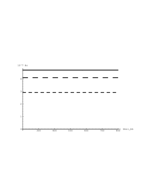
Refer to caption
Figure 1: $Br$ as a function of the mass $m_{H^{\pm}}$ for fixed $\bar{\xi}_{N,bb}^{D}=60\,m_{b}$ at the region $|r_{tb}|<<1$. Here solid lines correspond to the scale $\mu=2.5\,\,GeV$, dashed lines to $\mu=5\,\,GeV$ and small dashed lines to $\mu=m_{W}\,\,GeV$. The lines corresponding to the SM coincides with the lines we present here.
Refer to caption
Figure 2: The same as Fig 1, but at the region $r_{tb}>>1$. Dotted dashed lines correspond to the SM. Note that dotted dashed line almost coincides with the $m_{H}$ axis
Refer to caption
Figure 3: The same as Fig 1, but for fixed $\bar{\xi}_{N,bb}^{D}=90\,m_{b}$ value.
Refer to caption
Figure 4: The same as Fig 2, but for fixed $\bar{\xi}_{N,bb}^{D}=90\,m_{b}$ value.
Refer to caption
Figure 5: $Br$ as a function of the coupling $\bar{\xi}_{N,bb}^{D}$ for fixed $m_{H^{\pm}}=500\,GeV$ at the region $|r_{tb}|<<1$. Here solid lines correspond to the scale $\mu=2.5\,\,GeV$, dashed lines to $\mu=5\,\,GeV$ and small dashed lines to $\mu=m_{W}\,\,GeV$. The lines corresponding to the SM coincides with the lines we present here.
Refer to caption
Figure 6: The same as Fig 5 but at the region $r_{tb}>>1$.
Refer to caption
Figure 7: $R$ ratio as a function of the mass $m_{H^{\pm}}$ for fixed $\bar{\xi}_{N,bb}^{D}=60\,m_{b}$ at the region $|r_{tb}|<<1$. Here solid lines correspond to the scale $\mu=2.5\,\,GeV$, dashed lines to $\mu=5\,\,GeV$ and small dashed lines to $\mu=m_{W}\,\,GeV$. The lines corresponding to the SM coincides with the lines we present here.
Refer to caption
Figure 8: The same as FigΒ 7, but at the region $r_{tb}>>1$. Here solid curves (lines) correspond to the scale $\mu=2.5\,\,GeV$, dashed curves (lines) to $\mu=5\,\,GeV$ and small dashed curves (lines) to $\mu=m_{W}\,\,GeV$ for model III (SM).
Refer to caption
Figure 9: The same as FigΒ 8 but for fixed $\bar{\xi}_{N,bb}^{D}=100\,m_{b}$.
Refer to caption
Figure 10: $R$ ratio as a function of the coupling $\bar{\xi}_{N,bb}^{D}$ for fixed $m_{H^{\pm}}=500\,GeV$ at the region $|r_{tb}|<<1$. Here solid lines correspond to the scale $\mu=2.5\,\,GeV$, dashed lines to $\mu=5\,\,GeV$ and small dashed lines to $\mu=m_{W}\,\,GeV$. The lines corresponding to the SM coincides with the lines we present here.
Refer to caption
Figure 11: The same as Fig 7, but at the region $r_{tb}>>1$. Here solid curves (lines) correspond to the scale $\mu=2.5\,\,GeV$, dashed lines to $\mu=5\,\,GeV$ and small dashed lines to $\mu=m_{W}\,\,GeV$ for model III (SM).
Refer to caption
Figure 12: The same as Fig. 2 but including LD effects. The lines corresponding to the SM coincides almost with the $m_{H^{\pm}}$ axis.
Refer to caption
Figure 13: The same as Fig. 5 but including LD effects.
Refer to caption
Figure 14: The same as Fig. 6 but including LD effects.
Refer to caption
Figure 15: The same as Fig. 7 but including LD effects.
Refer to caption
Figure 16: The same as Fig. 8 but including LD effects.
Refer to caption
Figure 17: The same as Fig 11 , but including LD effects.