THE SMALL $x$ BEHAVIOR OF $g_{1}$ IN THE RESUMMED APPROACH

Abstract

The double logarithmic terms $\alpha_{s}\ln^{2}x$ are important to predict precisely the small $x$ behavior of the spin structure function $g_{1}$. We numerically analyze the evolution of the flavor non-singlet $g_{1}$ including the all-order resummed effect of these terms. It is pointed out that the next-to-leading logarithmic corrections produce an unexpectedly large suppression factor over the experimentally accessible range of $x$ and $Q^{2}$. This implies that the next-to-leading logarithmic contributions are very important in order to obtain a definite prediction.

1 Introduction

Recently many experimental and theoretical works have been devoted to the polarized structure function $g_{1}$. Especially, it is very important and desirable to know the small $x$ behavior of $g_{1}$ in the light of the Bjorken and Ellis-Jaffe sum rules. Since the verification of these sum rules requires the knowledge of the structure function over the entire $x$ regions, one has to rely on the theoretical prediction in the experimentally inaccessible small $x$ region. Although the Regge prediction has usually been assumed for the extrapolation of the experimental data to the small $x$ region, the recent data show a clear departure from this naive Regge prediction  [1]. This fact means that the perturbative QCD effects are very important.
   Recently, various extrapolations have been proposed using the DGLAP equation  [2]. However,it has been known that there appear the double logarithmic terms $\alpha_{s}ln^{2}x$ in the perturbative calculations. These logarithmic corrections seem to give large effects in the small $x$ region and are important to get more reliable predictions on the small $x$ behavior of $g_{1}$. Bartels, Ermolaev and Ryskin [3] have given the resummed expression for the partonic structure function $g^{parton}_{1}$ by using the Infra-Red Evolution Equation and confirmed the old result by Kirschner and Lipatov [4]. They claim that the resummed effects may be important. But, when extracting the physical structure function of hadrons from the partonic one, there is possibility that their conclusion at the parton level is not necessarily true. Indeed,the recent numerical analysis by Blümlein and Vogt [5] shows that there are no significant contributions from the resummation of the leading logarithmic (LL) corrections in the HERA kinematical region. The different conclusions between at the partonic and hadronic level might come from the fact that the resummed “coefficient function” was not included in Ref. [5] because it falls in the next-to-leading logarithmic (NLL) corrections and depends on the factorization scheme adopted. It is also to be noted that the slightly steep input density was used in Ref. [5]. The evolution, in general, strongly depends on the input parton densities. If one chooses a steep input function, the perturbative contribution will be completely washed away. So it will be also interesting to see the sensitivity of the results to the choice of the input densities.
   In this report, we reanalyze the numerical impact of the resummed effects on the small $x$ behavior of $g_{1}$ (non-singlet part). The coefficient function can not be included consistently at present since the anomalous dimension has been calculated only to the LL order. However we consider the effects of this part because we could firstly clarify an origin of the above different conclusions and secondly get some idea about the magnitude of the NLL order corrections in the resummation approach. We also consider two different input densities: one is flat corresponding to the naive Regge prediction and the other is steep in the small $x$ region. Details of the calculations may be found in Ref. [6].

2 Resummed structure function $g_{1}$

The flavor non-singlet part of $g_{1}$ in the moment space is given by,

$$g_{1}(Q^{2},N)\equiv\int^{1}_{0}dxx^{N-1}g_{1}(Q^{2},x)=\frac{\langle e^{2}\rangle}{2}C(\alpha_{s}(Q^{2}),N)\Delta q(Q^{2},N)\ ,$$

where

$$C(\alpha_{s}(Q^{2}),N)\equiv\int^{1}_{0}dxx^{N-1}C(\alpha_{s}(Q^{2}),x)\ \ ,\ \ \Delta q(Q^{2},N)\equiv\int^{1}_{0}dxx^{N-1}\Delta q(Q^{2},x)\ ,$$

and $\Delta q(Q^{2},x)$ ($C$) is the flavor non-singlet combination of the polarized parton densities (the coefficient function). $\langle e^{2}\rangle$ is the average of the quark’s electric charge. The DGLAP equation is,

$$Q^{2}\frac{\partial}{\partial Q^{2}}\Delta q(Q^{2},N)=-\gamma(\alpha_{s}(Q^{2}),N)\Delta q(Q^{2},N)\ .$$ (1)

Here the anomalous dimension $\gamma$ is the moment of the “splitting” function. The coefficient function $C(\alpha_{s},N)$ and the anomalous dimension $\gamma(\alpha_{s},N)$ can be calculated perturbatively and are expanded in the powers of $\alpha_{s}$,

$$C(\alpha_{s},N)=1+\sum_{k=1}^{\infty}c^{k}(N)\bar{\alpha}_{s}^{k}\ \ ,\ \ \gamma(\alpha_{s},N)=\sum_{k=1}^{\infty}\gamma^{k}(N)\bar{\alpha}_{s}^{k}\ .$$

where $\bar{\alpha}_{s}\equiv\frac{\alpha_{s}}{4\pi}$ . The singular behaviors of the anomalous dimension and the coefficient function as $x\to 0$ appear as the pole singularities at $N=0$. We must resum these singular terms to all orders to get a reliable prediction. This resummation has been done in Refs. [3] [4] and the resummed part of these functions are given as follows,

$$\hat{\gamma}(\alpha_{s},N) \equiv \lim_{N\to 0}\gamma(\alpha_{s},N)=-f^{-}_{0}(N)/8\pi^{2}\ ,$$ (2)

$$\hat{C}(\alpha_{s},N) \equiv \lim_{N\to 0}C(\alpha_{s},N)=\frac{N}{N-f^{(-)}_{0}(N)/8\pi^{2}}\ .$$ (3)

Here $f_{0}^{-}$ is given by,

$$f^{-}_{0}(N)=4\pi^{2}N\left(1-\sqrt{1-8C_{F}\frac{\bar{\alpha}_{s}}{N^{2}}\left[1-\frac{1}{2\pi^{2}N}f^{+}_{8}(N)\right]}\right)\ .$$

with

$$f^{+}_{8}(N)=16\pi^{2}N_{c}\bar{\alpha}_{s}\frac{d}{dN}\ln(e^{z^{2}/4}D_{-1/2N_{c}^{2}}(z))\quad,\quad z=\frac{N}{\sqrt{2N_{c}\bar{\alpha}_{s}}}\ .$$

$D_{p}(z)$ is the parabolic cylinder function. One can easily see by expanding Eqs.(2,3) in terms of $\alpha_{s}$ that the resummed expressions Eqs.(2,3) reproduce the known NLO results in the $\overline{\rm MS}$ scheme. Therefore, it is quite plausible that Eqs.(2,3) correctly sum up the “leading” singularities to all orders.
   Before going to the numerical analysis, we explain the reason why the resummed coefficient part was discarded in the analysis of Blümelein and Vogt. For definiteness, let us use the so-called DIS scheme. The parton density and the anomalous dimension in the DIS scheme are obtained by making the transformations,

$$\Delta q\rightarrow\Delta q^{DIS}\equiv C\Delta q\ \ ,\ \ \gamma^{DIS}\equiv C\gamma C^{-1}-\beta(\alpha_{s})\frac{\partial}{\partial\alpha_{s}}\ln C\ .$$ (4)

Using the resummed $\hat{\gamma}$ and $\hat{C}$ Eqs.(2,3), we get the anomalous dimension in the DIS scheme,

$$\hat{\gamma}^{DIS}=N\sum^{\infty}_{k=1}\hat{\gamma}^{k}\left(\frac{\bar{\alpha}_{s}}{N^{2}}\right)^{k}+\beta_{0}N^{2}\sum^{\infty}_{k=2}\hat{d}^{k}\left(\frac{\bar{\alpha}_{s}}{N^{2}}\right)^{k}+{\cal O}\left(N^{3}\left(\frac{\bar{\alpha}_{s}}{N^{2}}\right)^{k}\right)\ ,$$ (5)

where the second term comes from the resummed coefficient function and $\hat{d}^{k}$ are numerical numbers independent of $N$. Since the second term has an extra $N$ in comparison with the first term in the each power of $\alpha_{s}$, the resummed coefficient function belongs to the NLL order corrections in the context of the resummation approach. This is the reason why the LL analysis of Blümlein and Vogt dropped the resummed coefficient function. One must include the NLL order anomalous dimension, which has not yet been available, to perform a consistent analysis at the NLL level.

3 Numerical consideration

We show our numerical results. From Eq.(4), in DIS scheme, $g_{1}$ is given by

$$g_{1}(x,Q^{2})=\frac{\langle e^{2}\rangle}{2}\int_{c-i\infty}^{c+i\infty}\frac{dN}{2\pi i}x^{-N}\Delta q^{DIS}(N,Q^{2})$$ (6)

The DGLAP equation Eq.(1) is easily solved with anomalous dimension $\gamma^{DIS}$,

$$\Delta q^{DIS}(N,Q^{2})=\exp\left(-\int_{\alpha_{s}(Q_{0}^{2})}^{\alpha_{s}(Q^{2})}\frac{d\alpha_{s}}{\beta}\gamma^{DIS}\right)\Delta q^{DIS}(N,Q_{0}^{2}).$$

The anomalous dimension $\gamma^{DIS}$ which includes the resummed effects is obtained by using Eqs.(2,3 ) and the relation Eq.(4),

$$\gamma^{DIS}(N)=\bar{\alpha}_{s}\gamma^{1}(N)+\bar{\alpha}_{s}^{2}\gamma^{2}(N)+K(N,\alpha_{s})-\beta\frac{\partial}{\partial\alpha_{s}}\ln\left(1+\bar{\alpha}_{s}c^{1}+H(N,\alpha_{s})\right)\ ,$$ (7)

where $\gamma^{1,2}$ and $c^{1}$ are respectively the exact anomalous dimension and coefficient function at the one and two-loop fixed order perturbation theory. $K(N,\alpha_{s})$ ($H(N,\alpha_{s})$) is the resummed anomalous dimension Eq.(2) (the coefficient function Eq.(3)) with $k=1,2$ ($k=0,1$) terms being subtracted to avoid the double counting. Although the anomalous dimension at $N=1$ should vanish due to the conservation of the (non-singlet) axial vector current, the resummation of the leading singularities in $N$ does not respect this symmetry. One of prescriptions to restore this symmetry is [5],

$$K(N,\alpha_{s})\to K(N,\alpha_{s})(1-N)\ .$$

In order to estimate $g_{1}$, we must assume the appropriate function for the input density $\Delta q^{DIS}(N,Q_{0}^{2})$. The explicit parameterization we use is [2],

$$\Delta q^{DIS}(Q_{0}^{2},x)=N(\alpha,\beta,a)\eta x^{\alpha}(1-x)^{\beta}(1+ax)\ ,$$

where $N$ is a normalization factor such that $\int dxNx^{\alpha}(1-x)^{\beta}(1+ax)=1$ and $\eta=\frac{1}{6}g_{A}$ ($g_{A}=1.26$) in accordance with the Bjorken sum rule and we choose the input scale $Q_{0}^{2}=4GeV^{2}$. Note that the small $x$ behavior is controlled by the parameter $\alpha$. Since we are also interested in the sensitivity of the final results to the small $x$ behavior of input densities, we choose two types of the input densities A and B: A is a function which is flat at small $x$ ($x^{\alpha},\alpha\sim 0$), and B is slightly steep ($\alpha\sim-0.2$) . A and B correspond to the following values of parameters,

$$A\ (B)\ :\ \alpha=+0.0\ (-0.2)\ ,\ \beta=3.09\ (3.15)\ ,\ a=2.23\ (2.72)\ .$$

We put the flavor number $n_{f}=4$ and $\Lambda_{QCD}=0.23GeV$.
   Now, let us explain how to perform the Mellin inversion Eq.(6) which is an integral in the complex $N$-plane. The contour integration along the imaginary axis from $c-i\infty$ to $c+i\infty$ is numerically inconvenient due to the slow convergence of the integral in the large $|N|$ region. To get rid of this problem, we deformed the contour to the line which have an angle $\phi$ ($\phi>\pi/2$) from the real $N$ axis. By this change of the contour, we have a damping factor $\exp(|N|\ln(1/x)\cos\phi)$ which strongly suppresses the contribution from the large $|N|$ region. In the integration along this new contour, we will be able to cut the large $|N|$ region. Finally we have checked the stability of results by changing the contour parameter. One can find the details of this technique in Ref. [9].
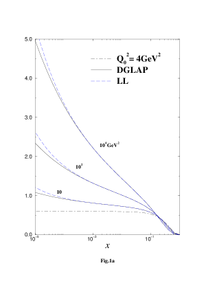
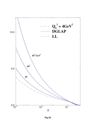
   First we estimate the case which includes only the LL correction. The evolution kernel in this case is obtained by dropping $H(N,\alpha_{s})$ in Eq.(7). Fig.1a (1b) shows the LL results (dashed curves) after evolving to $Q^{2}=10,10^{2},$ $10^{4}GeV^{2}$ from the A (B) input density (dot-dashed line). The solid curves are the predictions of the NLO-DGLAP evolution. These results show a tiny enhancement compared with the NLO-DGLAP analysis and are consistent with those in Ref. [5] The enhancement is, as expected, bigger when the input density is flatter. However any significant differences are not seen between the results from different input densities.

Figure 1: The LL evolution as compared to the DGLAP results with the flat input A (1a) and steep one B (1b).

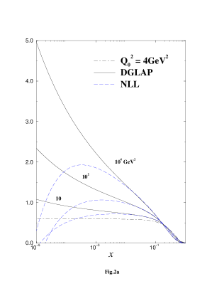
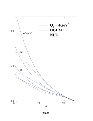
Next, we include the NLL corrections from the resummed “coefficient function”. We show the results in Fig.2 by the dashed curves. The results are rather surprising. The inclusion of the coefficient function leads to a strong suppression on the evolution of the structure function at small $x$.

Figure 2: The NLL evolution as compared to the DGLAP results with the flat input A (2a) and steep one B (2b).

To understand our numerical results, it will be helpful to remember the perturbative expansion of the resummed results Eqs.(2,3). Using the explicit values $N_{C}=3,C_{F}=4/3$, we obtain for the anomalous dimension in the DIS scheme Eq.(5),

$$\hat{\gamma}^{DIS} = N\left[-0.212\left(\frac{\alpha_{s}}{N^{2}}\right)\right.$$

$$\qquad-\,0.068\left.\left(\frac{\alpha_{s}}{N^{2}}\right)^{2}-0.017\left(\frac{\alpha_{s}}{N^{2}}\right)^{3}-0.029\left(\frac{\alpha_{s}}{N^{2}}\right)^{4}+\cdots\right]$$

$$+ \,N^{2}\left[0.141\left(\frac{\alpha_{s}}{N^{2}}\right)^{2}+0.119\left(\frac{\alpha_{s}}{N^{2}}\right)^{3}+0.069\left(\frac{\alpha_{s}}{N^{2}}\right)^{4}+\cdots\right]$$

$$+ \,\,\,\cdots\ \ .$$

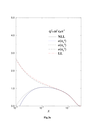
Here note that: (1) the perturbative coefficients of the LL terms (the first part of Eq.(3)) are negative and those of the higher orders are rather small number. This implies that the LL corrections push up the structure function compared to the fixed-order DGLAP evolution, but the deviations are expected to be small. (2) the perturbative ones from the NLL terms (the second part of Eq.(3)), however, are positive and somehow large compared with those of the LL terms. This positivity of the NLL terms has the effect of decreasing the structure function. It might be also helpful to assume that the saddle-point dominates the Mellin inversion Eq.(6). We have numerically estimated the approximate position of the saddle-point and found that the saddle-point stays around $N_{\rm SP}\sim 0.31$ in the region of $x\sim 10^{-5}$ to $10^{-2}$. By looking at the explicit values of the coefficients in Eq.(3), the position of the saddle-point seems to suggest that the NLL terms can not be neglected. Since the coefficients from the higher order terms are not so large numerically, it is also expected that the terms which lead to sizable effects on the evolution may be only first few terms in the perturbative series in the region of $x$ we are interested in.

Figure 3: Contributions from the fixed order terms in the NLL resummation with the flat input A (3a) and steep one B (3b).

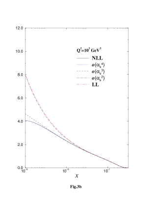Fig.3a (3b) shows the numerical results of the contribution from each terms of the NLL corrections in Eq.(3) at $Q^{2}=10^{2}GeV^{2}$ with the A (B) type input density. The solid (dot-dashed) line corresponds to the NLL (LL) result. The long-dashed, dashed and dotted lines correspond respectively to the case in which the terms up to the order $\alpha_{s}^{2}$, $\alpha_{s}^{3}$, $\alpha_{s}^{4}$, are kept in the NLL contributions. One can see that the dotted line already coincides with the full NLL (solid) line. These considerations could help us to understand why the NLL corrections turns out to give large effects.

4 summary

We have numerically studied the small $x$ behavior of the flavor non-singlet $g_{1}$ by taking into account the resummed effect of $\alpha_{s}ln^{2}x$. Our LL analysis is consistent with the results by Blümlein and Vogt [5]. We have also performed the analysis which includes a part of the NLL corrections from the resummed coefficient function in the light of the assertion of Bartels, Ermolaev and Ryskin [3], though this is not theoretically consistent. Our results suggest that the LL analysis is unstable in the sense that a large suppression effect comes from the resummed coefficient function which should be NLL corrections. We need a full NLL analysis to make a definite conclusion.

This work was supported in part by the Monbusho Grant-in-Aid Scientific Research No. A (1) 08304024, No. C (1) 09640364.

References

- [1] Y.Miyachi,Talk at this symposium; T.Shibata,Talk at this symposium; J.Lichtenstadt,Talk at this symposium.
- [2] G. Altarelli, R. D. Ball, S. Forte and G. Ridolfi, Nucl. Phys. B496 (1997) 337.
- [3] J. Bartels, B. I. Ermolaev and M. G. Ryskin, Z. Phys. C70 (1996) 273; ibid. C72 (1997) 627.
- [4] R. Kirschner and L. N. Lipatov, Nucl. Phys. B213 (1983) 122.
- [5] J. Blümlein and A. Vogt ,Phys. Lett. B370 (1996) 149 ; Acta.Phys.Polonica B27 (1996) 1309; J. Blümlein, S. Riemersma and A. Vogt, hep-ph/9608470.
- [6] Y. Kiyo, J. Kodaira and H. Tochimura, Z. Phys. C74 (1997) 631.;hep-ph/9711260.
- [7] J. Kodaira, S. Matsuda, T. Muta, K. Sasaki and T. Uematsu, Phys. Rev. D20 (1979) 627; J. Kodaira, S. Matsuda, K. Sasaki and T. Uematsu, Nucl. Phys. B159 (1979) 99.
- [8] R. Mertig and W. L. van Neerven, Z. Phys. C70 (1996) 637 and references therein.
- [9] M. Glück, E. Reya and A. Vogt, Z. Phys. C48 (1990) 471; D. Graudenz, M. Hampel, A. Vogt and Ch. Berger, Z. Phys. C70 (1996) 70.
- [10] R. D. Ball and S. Forte, Phys. Lett. B351 (1995) 313; J. R. Forshaw, R. G. Roberts and R. S. Thorne, Phys. Lett. B356 (1995) 79.