CERN-TH/98-70

HIP-1998-14/TH

hep-ph/9803367

March 1998

THERMODYNAMICS OF GAUGE-INVARIANT U(1) VORTICES
FROM LATTICE MONTE CARLO SIMULATIONS

K. Kajantie^a,b,, M. Karjalainen^b,, M. Laine^a,b,, J. Peisa^c,, and A. Rajantie^d,

^aTheory Division, CERN, CH-1211 Geneva 23, Switzerland

^bDepartment of Physics, P.O.Box 9, 00014 University of Helsinki, Finland

^cDepartment of Mathematical Sciences, University of Liverpool,
Liverpool L69 3BX, UK

^dHelsinki Institute of Physics, P.O.Box 9, 00014 University of Helsinki, Finland

Abstract

We study non-perturbatively and from first principles the thermodynamics of vortices in 3d U(1) gauge+Higgs theory, or the Ginzburg-Landau model, which has frequently been used as a model for cosmological topological defect formation. We discretize the system and introduce a gauge-invariant definition of a vortex passing through a loop on the lattice. We then study with Monte Carlo simulations the total vortex density, extract the physically meaningful part thereof, and demonstrate that it has a well-defined continuum limit. The total vortex density behaves as a pseudo order parameter, having a discontinuity in the regime of first order transitions and behaving continuously in the regime of second order transitions. Finally, we discuss further gauge-invariant observables to be measured.

PACS numbers: 98.80.Cq, 11.27.+d, 11.15.Ha, 67.40.Vs, 74.60.-w

1 Introduction

Vortices play a significant role from the low temperatures of liquid crystals [1], superfluids [2] and high-$T_{c}$ superconductors [3], to the relativistic temperatures of the Early Universe [4]. In low temperature systems, vortices can be directly observed [1, 5]; in cosmology, one has studied their effects on the inhomogeneities leading to structure formation [6]. Consequently, vortices have been a subject of immense interest during the last few years. Nevertheless, some important questions, related in particular to non-perturbative studies of vortices in gauge theories, remain poorly understood.

Among the most fundamental principles of Nature appear to be gauge invariance and spontaneous symmetry breaking, and already the simplest theory with these properties, the locally U(1) symmetric gauge+scalar quantum field theory or the Ginzburg-Landau (GL) model, contains vortices. The GL model does describe real physics in liquid crystals and superconductors [7], while in cosmology it is to be viewed as a simple toy model. The phase structure of the GL model is non-trivial: in the type I regime, there is a first order transition [8], whereas in the type II regime, the transition is assumed to be of the second order [9]–[12].

One of the mentioned open questions arises immediately when one realizes that the type II regime of the GL model is completely non-perturbative: perturbation theory does not describe the transition at all [13]. The only known systematic and controllable method for studying this regime are lattice Monte Carlo simulations [13]–[18]. Yet as to date, to our knowledge, the vortex density has not been studied in detail on the lattice even in thermodynamical equilibrium. The purpose of this paper is (a) to provide a gauge-invariant formulation for studying vortices on the lattice, (b) to measure the vortex density both in type I and type II regimes, and (c) to extrapolate the results to the infinite volume and continuum limits. The length distribution of vortices will be studied in a future publication [19]. In a U(1) scalar field theory without gauge symmetry, the thermodynamics of vortices has previously been addressed in [20].

Let us stress that considering the thermodynamics of vortices is certainly only a starting point. Ultimately one is interested in the real-time scaling properties of vortex networks created in a non-equilibrium situation (see, e.g., [21]–[23]). However, the thermodynamical equilibrium situation provides the initial conditions for such non-equilibrium processes. Furthermore, it is clear that non-equilibrium physics cannot be understood in quantitative detail before the equilibrium limit is under control.

2 The theory in the continuum and on the lattice

Let us start by defining the theory. The continuum theory is defined by the functional integral

$$Z = \int{\cal D}A_{i}{\cal D}\phi\,\exp\bigl{[}-S(A_{i},\phi)\bigr{]},$$ (1)

$$S = \int d^{3}x\biggl{[}{\frac{1}{4}}F_{ij}^{2}+|D_{i}\phi|^{2}+m_{3}^{2}\phi^{*}\phi+\lambda_{3}\left(\phi^{*}\phi\right)^{2}\bigg{]},$$ (2)

where $F_{ij}=\partial_{i}A_{j}-\partial_{j}A_{i}$ and $D_{i}=\partial_{i}+ie_{3}A_{i}$. The theory is invariant under the gauge transformations

$$\phi({\bf x})\to e^{i\theta({\bf x})}\phi({\bf x}),\quad A_{i}({\bf x})\to A_{i}({\bf x})-\partial_{i}\theta({\bf x})/e_{3}.$$ (3)

Writing $\phi(\mbox{\bf x})=v(\mbox{\bf x})\exp[i\gamma(\mbox{\bf x})]$, the first of these can be rewritten as $\gamma(\mbox{\bf x})\to[\gamma(\mbox{\bf x})+\theta(\mbox{\bf x})]_{\pi}$, where $[X]_{\pi}\equiv X+2\pi n$ such that $[X]_{\pi}\in(-\pi,\pi]$ and we have chosen to represent the phase of $\phi$ by a number in this interval. The theory in eq. (2) is parameterized by the scale $e_{3}^{2}$ and by the two dimensionless ratios

$$y={m_{3}^{2}(e_{3}^{2})\over e_{3}^{4}},\quad x={\lambda_{3}\over e_{3}^{2}},$$ (4)

where $m_{3}^{2}(\mu)$ is the mass parameter in the $\overline{\mbox{\rm MS}}$ dimensional regularization scheme in $3-2\epsilon$ dimensions. Expressions for $x$ and $y$ in terms of the original physical parameters of both 4d high temperature scalar+fermion electrodynamics and 3d low-$T_{c}$ superconductivity, have been discussed in [18] where we refer to for more details. Here we just study the theory as a function of $x,y$. The phase diagram is shown in Fig. 1.

Figure 1: The phase diagram of the GL model, together with the main simulation points (marked with the diamonds).

As is well known, the classical counterpart of the theory in eq. (2) admits vortex, or string solutions, in the broken (superconducting) phase. In other words, the classical equations of motion have solutions in which the symmetry is restored at the core, but is broken far away from the core [24]. The existence of a vortex inside a loop $C$ can be identified by computing the line integral

$$n_{C}=\frac{1}{2\pi}\oint_{C}\!d\mbox{\bf x}\cdot\nabla\gamma(\mbox{\bf x}),$$ (5)

where the winding number $n_{C}$ is an integer, and a non-zero $n_{C}$ signals a vortex inside the loop. It can be seen from eq. (3) that $n_{C}$ is gauge-invariant for single-valued gauge transformations $\theta(\mbox{\bf x})$. Thus vortices are physical objects, which can be generated in a phase transition or by applying non-trivial boundary conditions, and they can be observed in the superconducting phase. However, in the equilibrium state they are also created and destroyed by thermal fluctuations, and $\langle|n_{C}|\rangle$ gives their density both in the broken and in the symmetric phase. Moreover, it is expected that the behavior of vortices is qualitatively different in the two phases. As the dynamics is non-perturbative, it is then clear that it is very important to be able to study vortices with lattice simulations.

It should be noted here that one often assumes that in the regime of large $x$, the gauge fields are not essential and one can approximate the theory in eq. (2) by the 3d XY-model with a global U(1) symmetry, or its dual version (see, e.g., [13, 26, 27]) whose fundamental objects are the vortices. While these approximations simplify the problem significantly, their validity is uncertain for finite $x$. Thus we consider it essential to approach the problem directly with the original theory in eq. (2).

To allow for lattice simulations, the theory in eq. (2) has to be discretized. As usual, we introduce the link field $U_{i}(\mbox{\bf x})=\exp[iae_{3}A_{i}(\mbox{\bf x})]\equiv\exp[i\alpha_{i}(\mbox{\bf x})]$. Rescaling the continuum scalar field to a dimensionless lattice field by $\phi^{*}\phi\to\beta_{H}\phi^{*}\phi/2a$, the lattice action becomes

$$S = \beta_{G}\!\!\sum_{\mbox{\bf x},i<j}{\frac{1}{2}}\hat{F}_{ij}^{2}(\mbox{\bf x})-\beta_{H}\sum_{\mbox{\bf x},i}{\mbox{Re}}\,\phi^{*}(\mbox{\bf x})U_{i}(\mbox{\bf x})\phi(\mbox{\bf x}+\hat{i})$$ (6)

$$+\sum_{\mbox{\bf x}}\phi^{*}(\mbox{\bf x})\phi(\mbox{\bf x})+\beta_{R}\sum_{\mbox{\bf x}}\left[\phi^{*}(\mbox{\bf x})\phi(\mbox{\bf x})-1\right]^{2},$$

where $\hat{F}_{ij}(\mbox{\bf x})=\alpha_{i}(\mbox{\bf x})+\alpha_{j}(\mbox{\bf x}+\hat{i})-\alpha_{i}(\mbox{\bf x}+\hat{j})-\alpha_{j}(\mbox{\bf x})$. We use here the non-compact formulation for the gauge fields. The gauge transformation properties in eq. (3) go over into

$$\gamma(\mbox{\bf x}) \to [\gamma(\mbox{\bf x})+\theta(\mbox{\bf x})]_{\pi},$$

$$\alpha_{i}(\mbox{\bf x}) \to \alpha_{i}(\mbox{\bf x})+\theta(\mbox{\bf x})-\theta(\mbox{\bf x}+\hat{i}).$$ (7)

Discretization can be viewed as a different regularization scheme, and in order to describe the same continuum physics as in eq. (2), one has to make a 2-loop computation relating the counterterms [28]. As a result, the lattice couplings $\beta_{G},\beta_{H},\beta_{R}$ are determined from

$$\beta_{G}={1\over e_{3}^{2}a},\qquad\beta_{R}={x\beta_{H}^{2}\over 4\beta_{G}},$$ (8)

$$2\beta_{G}^{2}\left({1\over\beta_{H}}-3-{x\beta_{H}\over 2\beta_{G}}\right)=y-{3.1759115(1+2x)\beta_{G}\over 2\pi}$$ (9)

$$\hskip 28.45274pt-\frac{(-4+8x-8x^{2})(\log 6\beta_{G}+0.09)-1.1+4.6x}{16\pi^{2}}.$$

Thus for a given continuum theory depending on one scale $e_{3}^{2}$ and the two dimensionless parameters $y,x$, the use of a lattice introduces a regulator scale $a$, and eqs. (6)–(9) specify, up to terms of order $e_{3}^{2}a$, the corresponding lattice action. Note that the simulations in [29] correspond to $\beta_{R}\to\infty$, whereas according to eq. (8), $\beta_{R}\to 0$ in the continuum limit for any finite $x$ ($\beta_{H}\to 1/3$).

3 Gauge-invariant vortices

Consider now vortices. The naive discretization of eq. (5) gives the standard algorithm used in scalar theories without gauge fields. For each loop $C$ one would define the winding number $\tilde{n}_{C}$ of the phase $\gamma$ of the scalar field. However, any $\gamma(\mbox{\bf x})$ can be changed arbitrarily with a gauge transformation, see eq. (7). Thus the $\gamma(\mbox{\bf x})$’s are essentially random numbers, and $\tilde{n}_{C}$ does not contain any real information about the dynamics of the system. Indeed, the result for a loop around a single plaquette, $\tilde{N}_{1\times 1}\equiv\langle|\tilde{n}_{1\times 1}({\bf x})|\rangle$, would equal $1/3$ in the case of completely uncorrelated field values, and this is what we measure from lattice simulations for $\tilde{N}_{1\times 1}$, irrespective of the parameters of the theory (to be more precise, we always get $\tilde{N}_{1\times 1}=0.32(1)\ldots 0.33(1)$). Thus the quantity $\tilde{n}_{C}$ has to be rejected.

One solution sometimes used in the literature would be to fix the gauge, which makes $\tilde{n}_{C}$ non-trivial. However, its value depends crucially on the gauge chosen, and it is even possible to choose a gauge in which $\tilde{n}_{C}$ always vanishes. Therefore, we believe that it is important to use an explicitly gauge-invariant definition, in order to be able to interpret the results correctly.

Fortunately, the problem with $\tilde{n}_{C}$ is not one of principle, and a satisfactory definition can be given. For each positively directed link $l=({\bf x},{\bf x}+\hat{i})$ let us define

$$Y_{({\bf x},{\bf x}+\hat{i})}=[\alpha_{i}({\bf x})+\gamma({\bf x}+\hat{i})-\gamma({\bf x})]_{\pi}-\alpha_{i}({\bf x}).$$ (10)

For links with negative direction the sign of $Y_{l}$ is changed: $Y_{({\bf x},{\bf x}-\hat{i})}=-Y_{({\bf x}-\hat{i},{\bf x})}.$ Then, for each closed loop $C$, we can define

$$Y_{C}=\sum_{l\in C}Y_{l}\equiv 2\pi n_{C}.$$ (11)

This definition has four main properties:

(a) For any field configuration and any loop $C$, $n_{C}\in{\sf Z\!\!Z}$.

(b) Directly from eqs. (7), one can see that the part of $Y_{l}$ in the square brackets is gauge-invariant. The term $-\alpha_{i}({\bf x})$ is not, but when summed over a closed loop into $Y_{C}$, the gauge dependence cancels. Hence $Y_{C}$ is gauge-invariant.

(c) Since $Y_{C}$ is gauge-invariant, one can always tune the gauge used in the evaluation of the $Y_{l}$’s such that the fields appearing are perturbatively small. But then, in the continuum limit, $\alpha_{i}=e_{3}aA_{i}$ goes to zero and one gets the correct continuum limit containing only the phase of $\phi$.

(d) The quantity $Y_{C}$ is additive: if there is a loop $C$ consisting of the loops $A,B$, then $Y_{C}=Y_{A}+Y_{B}$. This is what one would require for counting the number of vortices going through loops of different sizes. This also implies that vortex lines cannot end, and therefore they form closed vortex loops. Note that we use a non-compact gauge field so that there are no monopoles.

Based on these properties, eq. (11) provides a valid formulation for counting vortices in the locally symmetric U(1) theory [30]. This definition of the winding number coincides with that given in Ref. [29] for the case $\beta_{R}=\infty$.

4 Simulations and results

In order to see how the gauge-invariant definition performs in practice, we have made lattice Monte Carlo simulations in the GL model. We choose $C=n\times n\equiv$ a loop around a plaquette of size $n\times n$ in eq. (11), and measure

$$N_{n\times n}\equiv\langle|n_{n\times n}|\rangle.$$ (12)

The quantity $N_{n\times n}$ measures the average net number of vortices through a loop of size $n\times n$, irrespective of the net direction. Keeping track of the direction would give zero: for symmetry reasons, $\langle n_{n\times n}\rangle=0$. In practice, we average $\langle|n_{n\times n}|\rangle$ over all lattice sites and directions, to improve on the statistics.

Simulations are made at two values of $x$: $x=0.0463$ corresponds to a strongly type I superconductor, $x=2$ to a strongly type II superconductor. For each $x$, values of $y$ are chosen on both sides of the transition (see Fig. 1). For each such continuum parameter point, several lattice spacings are chosen: $\beta_{G}=1/(e_{3}^{2}a)=1,2,3,4,6,8,12$. For $\beta_{G}=4$ ($x=0.0463$) and $\beta_{G}=1,2$ ($x=2$), several volumes are chosen, in order to test that the finite volume effects are small. The volumes thus arrived at (24${}^{2}\times$48 for $\beta_{G}=4$ both at $x=0.0463,x=2$) are then scaled with $\beta_{G}$ such that the physical volume (in units of $1/e_{3}^{6}$) remains constant. The orders of magnitude for $\beta_{G}$ and the volume come from the requirement that the physical correlation lengths, of order $(0.5\ldots 2)/e_{3}^{2}$ at $x=0.0463$ and $(1.5\ldots 3)/e_{3}^{2}$ at $x=2$ [17], are much longer than the lattice spacing but much shorter than the extent of the whole lattice (with the exception of the photon in the symmetric phase).

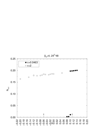
Figure 2: The values of $N_{1\times 1}$ at $x=0.0463$ and $x=2$, as a function of $y$. The transition points are indicated by the arrows. There is a discontinuity at the first order transition at $x=0.0463$, whereas in the regime of large $x$, $N_{1\times 1}$ behaves continuously. Some of the points at $x=0.0463$ correspond to metastable phases.

The results for $N_{1\times 1}$ as a function of $y$ are shown in Fig. 2. The two values of $x$ have a different critical point $y_{c}$, see Fig. 1. At small $x$ the vortex density is very small in the broken phase but jumps discontinuously to a large value at the transition. However, the symmetric-phase value $\approx 0.2$ is much smaller than the trivial value $1/3$. At large $x$ the behavior is completely different. The total vortex density is large also rather deep in the broken phase and there is no discontinuity at the transition.

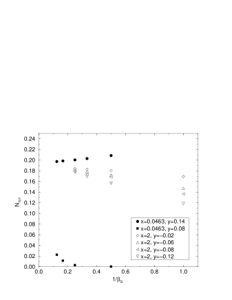
Figure 3: The continuum extrapolation of $N_{1\times 1}$ for different values of $x,y$. Even though there is a lot of structure at finite $\beta_{G}$, all results approach a single point in the continuum limit $\beta_{G}\to\infty$, including those in the broken phase. Both polynomial ($c_{0}+c_{1}/\beta_{G}+c_{2}/\beta_{G}^{2}$) and logarithmic ($c_{0}+c_{1}\ln\beta_{G}/\beta_{G}+c_{2}/\beta_{G}$) fits are allowed at $1/\beta_{G}\to 0$, the latter ones favouring a slightly larger $c_{0}\sim 0.20$.

Let us then discuss the approach to the continuum limit: $a\to 0$ and hence $\beta_{G}\to\infty$. The continuum extrapolation of $N_{1\times 1}$ is shown in Fig. 3. It is seen that even though there is a lot of structure at a finite $\beta_{G}$, all the structure disappears when $\beta_{G}\to\infty$ and one gets a result which is independent of the parameters of the continuum theory [31]. In the continuum limit, the loop of size $1\times 1$ (as well as a loop of any finite size $n\times n$ in lattice units) shrinks to a point, and it is clear that the result is merely an artifact of the lattice regularization, and sensitive only to UV-effects. Note that the continuum value $N_{1\times 1}\sim 0.2$ is close to the “universal” value seen, e.g., in [20] (there it was obtained at a fixed lattice spacing but at the point of a second order phase transition, which corresponds precisely to the continuum limit).

An important point to be noticed from Fig. 3 is that in the broken phase ($x=0.0463,y=0.08$), the asymptotic $\beta_{G}$ regime is obtained quite late, $\beta_{G}\mathop{\raise 1.29167pt\hbox{$>$\kern-7.5pt\raise-4.73611pt\hbox{$\sim$}}}8$. This is somewhat surprising since the smallest physical correlation length at this point is $1/m_{W}\sim 0.4/e_{3}^{2}$ [17], corresponding to $\sim 2.4a$ already at $\beta_{G}=6$. Thus one would expect to be approaching the continuum limit earlier. The Higgs correlation length is much larger, $1/m_{H}\sim 2/e_{3}^{2}\sim 12a$ at $\beta_{G}=6$.

For larger loops $n\times n$, the qualitative behaviour is similar to that for $N_{1\times 1}$, although the numerical values are different. For large $\beta_{G}$, including only terms linear in $a$, we expect the values of $N_{n\times n}$ to behave as

$$N_{n\times n}\approx f(n)+[d(x,y)+e(x,y)n]/\beta_{G}+{\cal O}(1/\beta_{G}^{2}).$$ (13)

In principle, there could be a $\ln\beta_{G}$-term in $d(x,y),e(x,y)$. For fixed $n$, the continuum value is $f(n)$, but it does not reflect the infrared dynamics of the theory. Fitting the data, the functional form of $f(n)$ is found to be consistent with $a+b/n+\bar{c}\ln n$ for large $n$. We cannot conclusively determine whether the coefficient $\bar{c}$ is non-vanishing or not. Assuming $\bar{c}=0$, we get $a\sim 0.33,b\sim-0.13$, but if $\bar{c}$ is allowed to be non-zero, the absolute values of $a$ and $b$ are somewhat smaller. The numerical determination of $\bar{c}$ is difficult, since it requires large values of $n$, for which very large lattices are needed to remove the finite size effects. In any case, the real physics lies in the coefficient of $1/\beta_{G}$ (see below), for which a fit of the form in eq. (13) works very well (the confidence level is CL=10–90%, depending on the parameter values $x,y$).

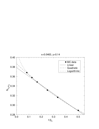
Figure 4: The continuum extrapolation of $N_{\beta_{G}\times\beta_{G}}$ at $x=0.0463,y=0.14$. Linear, quadratic and logarithmic fits are shown; the logarithmic one has the best confidence level, CL$=$11%. The value of $N_{\beta_{G}\times\beta_{G}}$ in the continuum limit is dominated by an unphysical regularization sensitive constant part, see the text.

Let us then discuss loops which are of a fixed size in physical units: $(c/e_{3}^{2})\times(c/e_{3}^{2})$, where $c$ is a constant. In lattice units this loop is $c\beta_{G}\times c\beta_{G}$, i.e., the size is varied as a function of $\beta_{G}$. The continuum extrapolation for the loop $N_{\beta_{G}\times\beta_{G}}$ ($c=1$) is shown in Fig. 4 at the point $x=0.0463,y=0.14$. According to eq. (13), we expect that in the continuum limit,

$$N_{(c\beta_{G})\times(c\beta_{G})}\approx\lim_{\beta_{G}\to\infty}f(c\beta_{G})+ce(x,y)+{\cal O}(c^{2}).$$ (14)

The first term is unphysical and corresponds to the regularization effects in eq. (15) below. (If there is a term $\ln\beta_{G}$ in $e(x,y)$, then the regularization sensitive part can also depend on $x,y$, but this dependence is analytic and does not affect any phase transitions.) Thus the absolute value of $N_{(c\beta_{G})\times(c\beta_{G})}$ is not physical, only its changes are (see Fig. 5). The physical effects, i.e. $ce(x,y)+{\cal O}(c^{2})$, come form the coefficient of $1/\beta_{G}$ (and ${\cal O}(1/\beta_{G}^{2})$) in eq. (13). To understand better the behaviour in eq. (14), let us discuss observables simpler than $n_{C}$.

Consider a typical composite operator, such as $\langle\phi^{*}\phi\rangle$. For $\langle\phi^{*}\phi\rangle$, one can make a perturbative computation to find out what happens in the continuum limit. It turns out the there is a linear (1-loop) and logarithmic (2-loop) divergence. The finite $\overline{\mbox{\rm MS}}$-scheme continuum result $\langle\phi^{*}\phi(e_{3}^{2})\rangle_{\mbox{\scriptsize cont}}$ is [28]

$${\langle\phi^{*}\phi(e_{3}^{2})\rangle_{\mbox{\scriptsize cont}}\over e_{3}^{2}}={\frac{1}{2}}\beta_{H}\beta_{G}\langle\phi^{*}\phi\rangle_{\mbox{\scriptsize latt}}-{3.1759115\beta_{G}\over 4\pi}-{1\over 8\pi^{2}}\biggl{[}\log(6\beta_{G})+0.668\biggr{]},$$ (15)

where “latt” refers to the normalisation of the field in the lattice action (6). The second term on the RHS is the linear, and the third the logarithmic divergence. The value of $\langle\phi^{*}\phi\rangle_{\mbox{\scriptsize latt}}$ measured on the lattice is thus not in itself a physical quantity: only its changes (such as the discontinuity across a first order transition) are, since in them the divergent parts cancel.

We now expect that a similar thing happens for $n_{C}$. The difference is that $n_{C}$ is a more complicated and non-local quantity. The regularization sensitive part is not easily computable in perturbation theory, since even the integral

$$N_{C}^{\rm free}=\int{\cal D}\phi\,|n_{C}|\exp\Bigl{(}-\int d^{3}x|\partial_{i}\phi|^{2}\Bigr{)}$$ (16)

is not Gaussian, due to the non-polynomial expression of $|n_{C}|$. A numerical evaluation of $N_{C}^{\rm free}$ (a mass term has to be included on the lattice to kill a zero mode) gives a result close to the fitted values of $f(n)$ in eq. (13) (and favours $\bar{c}=0$).

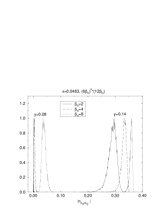
Figure 5: The distributions of the volume average of $|n_{\beta_{G}\times\beta_{G}}|$ for values of $y$ just below and above the critical point $y_{c}$ at $x=0.0463$. Precisely at $y_{c}$, the two peaks would appear simultaneously.

To demonstrate that the changes in $N_{\beta_{G}\times\beta_{G}}$ are physical, the distributions of $N_{\beta_{G}\times\beta_{G}}$ at $x=0.0463,\beta_{G}=2,4,8$ around the first order phase transition are shown in Fig. 5. It is seen that the two-peak structure (in particular, the distance between the peaks) indeed remains the same within statistical errors when $\beta_{G}$ is varied, when $\beta_{G}$ is large enough ($\beta_{G}=4,8$). Thus the two-peak structure is physical and has a finite continuum limit, while the location of the structure on the $|n_{\beta_{G}\times\beta_{G}}|$-axis is unphysical and dominated by UV-effects: both peaks move to the right when $\beta_{G}$ increases (the location of the $y=0.14$ peak is shown in Fig. 4). Note that $\beta_{G}=2$ is not yet in the scaling regime, and thus the distance between the peaks is different from that at $\beta_{G}=4,8$.

For $x=2$, there is only a single peak which moves continuously to larger values as $y$ is increased, see Fig. 2.

5 Conclusions

In conclusion, we have given a gauge-invariant definition for a vortex passing through a loop on a lattice, measured the corresponding total vortex density, and discussed its extrapolation to the continuum limit. We have pointed out that to approach a meaningful continuum limit, one must keep the size of the loop fixed in physical units. We have found that the total vortex density behaves as a pseudo order parameter, analogously to $\langle\phi^{*}\phi\rangle$: the absolute value is always non-zero and is dominated by regularization effects near the continuum limit. Thus only the changes of the total vortex density with respect to the continuum parameters are physically meaningful. In the type I regime, the total vortex density displays a discontinuity, whereas in the type II regime, it behaves smoothly as the phase transition is crossed (Fig. 2).

The system possesses also (non-local) observables which behave analogously to true order parameters. One such is the photon mass, which vanishes exactly in the symmetric phase. It has been suggested that another such quantity might be the density of long vortices passing through the whole lattice [25, 20]. In contrast to the photon mass, this quantity should vanish in the broken phase and remain non-zero in the symmetric phase. The measurement of the density of long vortices is in progress [19].

Finally, it would be interesting to study the spatial distribution of vortices. This can be done by measuring correlators of “vortex density operators” $n_{C}$, separated by a distance $r$. One can define several correlators, depending on the relative orientations of the loops used in the $n_{C}$’s. These quantities would give realistic initial conditions for simulations of the time evolution of vortex networks.

References

- [1] I. Chuang, R. Durrer, N. Turok, and B. Yurke, Science 251 (1991) 1336; M.J. Bowick, L. Chandar, E.A. Schiff, and A. M. Srivastava, Science 263 (1994) 943.
- [2] W.H. Zurek, Phys. Rept. 276 (1996) 177.
- [3] G. Blatter, M.V. Feigel’man, V.B. Geshkenbein, A.I. Larkin and V.M. Vinokur, Rev. Mod. Phys. 66 (1994) 1125.
- [4] A. Vilenkin and E.P.S. Shellard, Cosmic Strings and Other Topological Defects (Cambridge University Press, 1994); M.B. Hindmarsh and T.W.B. Kibble, Rept. Prog. Phys. 58 (1995) 477.
- [5] P.C. Hendry, N.S. Lawson, R.A.M. Lee, P.V.E. McClintock, and C.H.D. Williams, Nature 368 (1994) 315; V.M.H. Ruutu, V.B. Eltsov, A.J. Gill, T.W.B. Kibble, M. Krusius, Yu.G. Makhlin, B. Placais, G.E. Volovik, and Wen Xu, Nature 382 (1996) 334; C. Bäuerle, Yu.M. Bunkov, S.N. Fischer, H. Godfrin, and G.R. Pickett, Nature 382 (1996) 332; V.M.H. Ruutu, V.B. Eltsov, M. Krusius, Yu.G. Makhlin, B. Placais, and G.E. Volovik, Phys. Rev. Lett. 80 (1998) 1465.
- [6] T.W.B. Kibble, J. Phys. A 9 (1976) 1387; Phys. Rep. 67 (1980) 183; U.-L. Pen, U. Seljak and N. Turok, Phys. Rev. Lett. 79 (1997) 1611.
- [7] H. Kleinert, Gauge Fields in Condensed Matter (World Scientific, 1989).
- [8] B.I. Halperin, T.C. Lubensky and S.-K. Ma, Phys. Rev. Lett. 32 (1974) 292.
- [9] J. March-Russell, Phys. Lett. B 296 (1992) 364.
- [10] B. Bergerhoff, F. Freire, D.F. Litim, S. Lola and C. Wetterich, Phys. Rev. B 53 (1996) 5734.
- [11] M. Kiometzis, H. Kleinert and A.M.J. Schakel, Phys. Rev. Lett. 73 (1994) 1975; H. Kleinert and A.M.J. Schakel, supr-con/9606001; cond-mat/9702159.
- [12] I. Herbut and Z. Tešanović, Phys. Rev. Lett. 76 (1996) 4588; I.F. Herbut, J. Phys. A: Math. Gen. 30 (1997) 423 [cond-mat/9610052]; cond-mat/9702167.
- [13] C. Dasgupta and B.I. Halperin, Phys. Rev. Lett. 47 (1981) 1556.
- [14] J. Bartholomew, Phys. Rev. B 28 (1983) 5378.
- [15] Y. Munehisa, Phys. Lett. B 155 (1985) 159.
- [16] P. Dimopoulos, K. Farakos and G. Kotsoumbas, Eur. Phys. J. C 1 (1998) 711.
- [17] K. Kajantie, M. Karjalainen, M. Laine and J. Peisa, Phys. Rev. B 57 (1998) 3011 [cond-mat/9704056].
- [18] K. Kajantie, M. Karjalainen, M. Laine and J. Peisa, Nucl. Phys. B, in press [hep-lat/9711048].
- [19] K. Kajantie, M. Laine, T. Neuhaus, J. Peisa and A. Rajantie, in progress.
- [20] N.D. Antunes, L.M.A. Bettencourt and M. Hindmarsh, Phys. Rev. Lett. 80 (1998) 908.
- [21] T. Vachaspati, CWRU-P18-97 [hep-ph/9710292].
- [22] P. Laguna and W.H. Zurek, Phys. Rev. Lett. 78 (1997) 2519; CGPG-97-12-1 [hep-ph/9711411]; A. Yates and W.H. Zurek, hep-ph/9801223.
- [23] G. Vincent, N.D. Antunes and M. Hindmarsh, Phys. Rev. Lett. 80 (1998) 2277.
- [24] H.B. Nielsen and P. Olesen, Nucl. Phys. B 61 (1973) 45.
- [25] A. Hulsebos, LTH-324 [hep-lat/9406016].
- [26] A. Kovner, B. Rosenstein and D. Eliezer, Nucl. Phys. B 350 (1991) 325; A. Kovner, P. Kurzepa and B. Rosenstein, Mod. Phys. Lett. A 14 (1993) 1343.
- [27] M. Kiometzis, H. Kleinert and A.M.J. Schakel, Fortschr. Phys. 43 (1995) 697.
- [28] M. Laine, Nucl. Phys. B 451 (1995) 484 [hep-lat/9504001]; M. Laine and A. Rajantie, Nucl. Phys. B 513 (1998) 471 [hep-lat/9705003].
- [29] J. Ranft, J. Kripfganz and G. Ranft, Phys. Rev. D 28 (1983) 360; M.N. Chernodub, M.I. Polikarpov and M.A. Zubkov, Nucl. Phys. B (Proc. Suppl.) 34 (1994) 256 [hep-lat/9401027]; M. Chavel, Phys. Lett. B 378 (1996) 227 [hep-lat/9603005].
- [30] A. Rajantie, Talk given in Quantum Phenomena at Low Temperatures, Helsinki, Jan 7–11, 1998 [cond-mat/9803221].
- [31] We thank G.D. Moore for demonstrating that the number can be obtained numerically by simulating the free scalar theory in eq. (16).