Magnetic and axial vector form factors as probes of
orbital angular momentum in the proton

Abstract

We have recently examined the static properties of the baryon octet (magnetic moments and axial vector coupling constants) in a generalized quark model in which the angular momentum of a polarized nucleon is partly spin $\langle S_{z}\rangle$ and partly orbital $\langle L_{z}\rangle$. The orbital momentum was represented by the rotation of a flux-tube connecting the three constituent quarks. The best fit is obtained with $\langle S_{z}\rangle=0.08\pm 0.15$, $\langle L_{z}\rangle=0.42\pm 0.14$. We now consider the consequences of this idea for the $q^{2}$-dependence of the magnetic and axial vector form factors. It is found that the isovector magnetic form factor $G_{M}^{\mathrm{isovec}}(q^{2})$ differs in shape from the axial form factor $F_{A}(q^{2})$ by an amount that depends on the spatial distribution of orbital angular momentum. The model of a rigidly rotating flux-tube leads to a relation between the magnetic, axial vector and matter radii, $\langle r^{2}\rangle_{\mathrm{mag}}=f_{\mathrm{spin}}\langle r^{2}\rangle_{\mathrm{axial}}+\frac{5}{2}f_{\mathrm{orb}}\langle r^{2}\rangle_{\mathrm{matt}}$, where $f_{\mathrm{orb}}/f_{\mathrm{spin}}=\frac{1}{3}\langle L_{z}\rangle/G_{A}$, $f_{\mathrm{spin}}+f_{\mathrm{orb}}=1$. The shape of $F_{A}(q^{2})$ is found to be close to a dipole with $M_{A}=0.92\pm 0.06$ GeV.

I Introduction

In a recent paper [1] we performed a fit to the magnetic moments of the baryon octet in a model in which these quantities are determined partly by the quark spins $\Delta u$, $\Delta d$, $\Delta s$, and partly by an orbital angular momentum $\langle L_{z}\rangle$, shared between the constituent quarks. The model is exemplified by the following ansatz for the proton and neutron magnetic moments: $\displaystyle\mu_{p}$ $\displaystyle=$ $\displaystyle\mu_{u}\Delta u+\mu_{d}\Delta d+\mu_{s}\Delta s+\left[\frac{2}{3}\mu_{u}+\frac{1}{3}\mu_{d}\right]\langle L_{z}\rangle,$ $\displaystyle\mu_{n}$ $\displaystyle=$ $\displaystyle\mu_{u}\Delta d+\mu_{d}\Delta u+\mu_{s}\Delta s+\left[\frac{1}{3}\mu_{u}+\frac{2}{3}\mu_{d}\right]\langle L_{z}\rangle.$ The part containing $\Delta u$, $\Delta d$, $\Delta s$, is the “spin” contribution to the magnetic moments, arising from the polarization of quarks and antiquarks in a polarized proton:

$$\Delta q=(q_{+}-q_{-})+(\bar{q}_{+}-\bar{q}_{-}).$$ (2)

The part proportional to $\langle L_{z}\rangle$ is the “orbital” (or convective) contribution, determined by the prescription of dividing the orbital angular momentum in proportion to the constituent quark masses. The complete set of baryon magnetic moments obtained by this prescription is shown in table I. These expressions, without the orbital part, were written down in Refs. [2, 3].

There are two essential elements that go into the above equations for the magnetic moments:

• It is assumed that one may use the quark spins $\Delta q$ in place of the quantities

  $$\delta q=(q_{+}-q_{-})-(\bar{q}_{+}-\bar{q}_{-})$$ (3)

  that are appropriate to an expression for the magnetic moment. This approximation is justified if antiquarks in a proton carry little polarization. An example of such a situation is the chiral quark model [4], in which antiquarks are embedded in a cloud of spin-zero mesons.

• The partition of $\langle L_{z}\rangle$ in proportion to the masses of the constituent quarks is based on the picture of a baryon as a symmetric three-pronged flux-tube of equal segments (fig.1), rotating collectively around the spin axis [1]. The appearence of the same magnetons $\mu_{u}$, $\mu_{d}$, $\mu_{s}$, in the orbital as in the spin part means, in particular, that the orbital $g$-factor has been taken to be $g_{l}=1$. (In a more general description, one could interpret $\langle L_{z}\rangle$ as $\langle g_{l}L_{z}\rangle$.)

II $S_{z}$ and $L_{z}$ from static properties

The fit to the empirical values of the magnetic moments in [1] was carried out under the following constraints:

• The quark magnetic moments were assumed to satisfy $\mu_{u}=-2\mu_{d}$, $\mu_{s}=0.6\mu_{d}$.

• The quark spins $\Delta u$, $\Delta d$ and $\Delta s$ were constrained to satisfy the measured values of the axial vector couplings $a^{(3)}$ and $a^{(8)}$:
  $\displaystyle a^{(3)}$ $\displaystyle=$ $\displaystyle\Delta u-\Delta d=1.26$ $\displaystyle a^{(8)}$ $\displaystyle=$ $\displaystyle\Delta u+\Delta d-2\Delta s=0.58$ These conditions are equivalent to the statement $F=0.46$, $D=0.80$, in terms of which $a^{(3)}=F+D$ ($\equiv G_{A}$, the axial vector coupling constant of neutron decay) and $a^{(8)}=3F-D$.

• Each magnetic moment was assigned a theoretical uncertainty of $\pm 0.1\mu_{N}$ (as in Ref.[2]). This ensured that all of the baryons were given essentially the same weight in the fit and the $\chi^{2}$ per degree of freedom was about unity.

In this manner, the magnetic moments are reduced to functions of three variables, which we choose to be $\mu_{u}$, $\langle L_{z}\rangle$ and $\langle S_{z}\rangle$, the last being defined as

$$\langle S_{z}\rangle=\frac{1}{2}\left(\Delta u+\Delta d+\Delta s\right)\equiv\frac{1}{2}\Delta\Sigma.$$ (5)

The result of the fit is

$$\mu_{u}=2.16\pm 0.08,\qquad\langle S_{z}\rangle=0.076\pm 0.13,\qquad\langle L_{z}\rangle=0.42\pm 0.10$$ (6)

with $\chi^{2}$/DOF = 1.1. For the central value of $\mu_{u}$, the allowed domain of $\langle S_{z}\rangle$ and $\langle L_{z}\rangle$ is given by the ellipse shown in fig.2. Allowing $\mu_{u}$ to vary over the interval given in eq.(6), we obtain the domain shown in fig.3, from which we infer a final estimate

$$\langle S_{z}\rangle=0.08\pm 0.15,\qquad\langle L_{z}\rangle=0.42\pm 0.14.$$ (7)

It is remarkable that the domain of $\langle S_{z}\rangle$ and $\langle L_{z}\rangle$ determined by the static properties of the baryons fulfils rather closely the condition $\langle S_{z}\rangle+\langle L_{z}\rangle=\frac{1}{2}$. That is, the spin and orbital momenta of the quarks and antiquarks saturate the angular momentum of the proton, without imposing this as an external requirement. This may be regarded as a posteriori justification for the assumption $g_{l}=1$. The fact that $\langle S_{z}\rangle+\langle L_{z}\rangle\approx\frac{1}{2}$ supports the idea, that the spin and orbital angular momentum are linked together by a transition of the form $q_{+}\to q^{\prime}_{-}+M$ ($L=1$), $M$ being a spin-zero meson [4]. This in turn provides support to the assumption $\delta q\approx\Delta q$, based on negligible antiquark polarization.

Also indicated in fig.3 is the location of two “sign-posts”, that serve as reference points in the angular momentum structure:

• NQM: This is the “naive quark model”, which describes the nucleon as 3 independent quarks in $1s$ orbits, corresponding to $\langle S_{z}\rangle=\frac{1}{2}$, $\langle L_{z}\rangle=0$. The $SU(6)$ symmetry of the model leads to the prediction $\Delta u=\frac{4}{3}$, $\Delta d=-\frac{1}{3}$, $\Delta s=0$, axial vector couplings $a^{(3)}=\frac{5}{3}$, $a^{(8)}=1$, and the magnetic moment ratio $\mu_{p}/\mu_{n}=-\frac{3}{2}$.

• QPM ($\Delta s=0$): This is the special case of the quark parton model discussed in Ref. [5], in which $\Delta u$ and $\Delta d$ were allowed to be free, but $\Delta s$ was neglected. The characteristic prediction of this model is $a^{(8)}=a^{(0)}$, where $a^{(0)}=\Delta u+\Delta d+\Delta s$, implying $\langle S_{z}\rangle=\frac{1}{2}a^{(0)}=\frac{1}{2}(3F-D)=0.29$, the remaining angular momentum being attributed to $\langle L_{z}\rangle=\frac{1}{2}-\langle S_{z}\rangle=0.21$. This version of the QPM leads to the Ellis-Jaffe sum rules [6] for polarized structure functions:

  $$\int g_{1}^{p}(x)dx=\frac{1}{2}\left(F-\frac{1}{9}D\right),\qquad\int g_{1}^{n}(x)dx=\frac{1}{3}\left(F-\frac{2}{3}D\right).$$ (8)

In what follows, we consider a test for the presence of orbital angular momentum $\langle L_{z}\rangle$ and its specific association with the collective rotation of the constituent quarks.

III Tests for $L_{z}$ in magnetic and axial vector form factors

We focus on the isovector magnetic moment of the nucleon, obtained by taking the difference of $\mu_{p}$ and $\mu_{n}$ in eq.(LABEL:mupmun):

$$\mu_{p}-\mu_{n}=\left(\mu_{u}-\mu_{d}\right)\left[G_{A}+\frac{1}{3}\langle L_{z}\rangle\right].$$ (9)

Note that the terms containing $\Delta s$ cancel in the difference. We regard this equation as a decomposition of the isovector magnetic moment into a part depending on the axial vector charge and a part depending on orbital angular momentum. Introducing the abbreviation

$$f_{\mathrm{spin}}\equiv\frac{\mu_{u}-\mu_{d}}{\mu_{p}-\mu_{n}}G_{A},\qquad f_{\mathrm{orb}}\equiv\frac{\mu_{u}-\mu_{d}}{\mu_{p}-\mu_{n}}\frac{1}{3}\langle L_{z}\rangle,$$ (10)

eq.(9) amounts to

$$1=f_{\mathrm{spin}}+f_{\mathrm{orb}}.$$ (11)

Returning to the three-parameter fit given by eq.(6), we can regard the fitted parameters as being $\langle S_{z}\rangle$, $f_{\mathrm{spin}}$ and $f_{\mathrm{orb}}$ (in place of $\langle S_{z}\rangle$, $\mu_{u}$ and $\langle L_{z}\rangle$). For the central value of $\langle S_{z}\rangle$, the domain of $f_{\mathrm{spin}}$ and $f_{\mathrm{orb}}$ determined by the various magnetic moments is shown in fig. 4. The fitted values, taking into account the spread of $\langle S_{z}\rangle$, are $f_{\mathrm{spin}}=0.87\pm 0.03$, $f_{\mathrm{orb}}=0.096\pm 0.03$. Considering that these values nearly satisfy the isovector magnetic moment relation, $f_{\mathrm{spin}}+f_{\mathrm{orb}}=1$, we use the following approximate values, which fulfil eq.(11) exactly

$$f_{\mathrm{spin}}=0.90\pm 0.03,\qquad f_{\mathrm{orb}}=0.10\pm 0.03.$$ (12)

Note that the ratio $f_{\mathrm{orb}}/f_{\mathrm{spin}}=\frac{\langle L_{z}\rangle}{3G_{A}}=\frac{1}{9}$ implies $\langle L_{z}\rangle=0.42$, as given in eq.(6). Eq.(12) amounts to the statement, that the isovector magnetic moment is 90% due to quark spin polarization and 10% due to quark rotation.

We now define spatial distributions $\rho_{\mathrm{mag}}(r)$, $\rho_{\mathrm{axial}}(r)$ and $\rho_{\mathrm{orb}}(r)$ whose volume integrals yield the quantities ($\mu_{p}-\mu_{n}$), $G_{A}$ and $\langle L_{z}\rangle$ appearing in eq.(9):

$$\mu_{p}-\mu_{n} = \int d^{3}x\,\rho_{\mathrm{mag}}(r),$$ (13)

$$G_{A} = \int d^{3}x\,\rho_{\mathrm{axial}}(r),$$ (14)

$$\langle L_{z}\rangle = \int d^{3}x\,\rho_{\mathrm{orb}}(r).$$ (15)

The local form of eq.(9) then reads

$$\rho_{\mathrm{mag}}(r)=\left(\mu_{u}-\mu_{d}\right)\left[\rho_{\mathrm{axial}}(r)+\frac{1}{3}\rho_{\mathrm{orb}}(r)\right].$$ (16)

Introducing, for convenience, “ normalized” densities

$$\tilde{\rho}_{\mathrm{mag}}(r) \equiv \rho_{\mathrm{mag}}(r)/(\mu_{p}-\mu_{n}),$$ (17)

$$\tilde{\rho}_{\mathrm{axial}}(r) \equiv \rho_{\mathrm{axial}}(r)/G_{A},$$ (18)

$$\tilde{\rho}_{\mathrm{orb}}(r) \equiv \rho_{\mathrm{orb}}(r)/\langle L_{z}\rangle,$$ (19)

eq.(16) assumes the form

$$\tilde{\rho}_{\mathrm{mag}}(r)=f_{\mathrm{spin}}\,\tilde{\rho}_{\mathrm{axial}}(r)+f_{\mathrm{orb}}\,\tilde{\rho}_{\mathrm{orb}}(r).$$ (20)

The functions $\tilde{\rho}_{\mathrm{i}}(r)$ all satisfy $\int\tilde{\rho}_{\mathrm{i}}(r)d^{3}x=1$, so that the integrated form of eq.(20) is simply the relation (11). Fourier transforming eq.(20), we get a relation between the isovector magnetic, axial vector and “orbital” form factors of the nucleon:

$$H_{\mathrm{mag}}^{\mathrm{isovec}}(Q^{2})=f_{\mathrm{spin}}\,H_{\mathrm{axial}}(Q^{2})+f_{\mathrm{orb}}\,H_{\mathrm{orb}}(Q^{2})$$ (21)

where

$$H_{\mathrm{i}}(Q^{2}=\vec{Q}^{2})=\int\,\tilde{\rho}_{\mathrm{i}}(r)\,e^{i\vec{Q}\vec{x}}d^{3}x$$ (22)

with $H_{\mathrm{i}}(0)=1$.

The form factor $H_{\mathrm{mag}}^{\mathrm{isovec}}(Q^{2})$ is an experimentally measured quantity, related to the magnetic (Sachs) form factors of the proton and the neutron by

$$H_{\mathrm{mag}}^{\mathrm{isovec}}(Q^{2})=\frac{G_{M}^{p}(Q^{2})-G_{M}^{n}(Q^{2})}{\mu_{p}-\mu_{n}}.$$ (23)

To the extent that $G_{M}^{p}(Q^{2})$ and $G_{M}^{n}(Q^{2})$ are both proportional to $(1+Q^{2}/0.71\,\mathrm{GeV}^{2})^{-2}$, we have

$$H_{\mathrm{mag}}^{\mathrm{isovec}}(Q^{2})=\frac{1}{\left(1+\frac{Q^{2}}{M_{V}^{2}}\right)^{2}},\qquad M_{V}=0.84\mathrm{GeV}.$$ (24)

The (normalized) axial vector form factor is likewise usually parametrized as a dipole

$$H_{\mathrm{axial}}(Q^{2})=\frac{1}{\left(1+\frac{Q^{2}}{M_{A}^{2}}\right)^{2}}.$$ (25)

It is clear from eq.(21), that the difference between $H_{\mathrm{mag}}^{\mathrm{isovec}}(Q^{2})$ and $H_{\mathrm{axial}}(Q^{2})$ is a measure of the orbital contribution proportional to $f_{\mathrm{orb}}$: in the limit $f_{\mathrm{orb}}=0$, $f_{\mathrm{spin}}=1$, these two form factors would be identical and we would have $M_{A}\equiv M_{V}$.

The orbital form factor $H_{\mathrm{orb}}(Q^{2})$ is a calculable feature of our model, which ascribes the orbital angular momentum to the rigid rotation of a flux-tube. Assuming matter in the proton to be distributed as $\rho_{\mathrm{matt}}\propto e^{-r/a}$, the density of orbital angular momentum $\tilde{\rho}_{\mathrm{orb}}$ is proportional to $r^{2}e^{-r/a}$. The resulting orbital form factor is

$$H_{\mathrm{orb}}(Q^{2}=\vec{Q}^{2})=\frac{\int e^{i\vec{Q}\vec{x}}\,r^{2}\,e^{-r/a}\,d^{3}x}{\int r^{2}\,e^{-r/a}\,d^{3}x}=\frac{1-Q^{2}a^{2}}{\left(1+Q^{2}a^{2}\right)^{4}}.$$ (26)

In particular, the rms radius associated with the orbital form factor is

$$\langle r^{2}\rangle_{\mathrm{orb}}=\frac{30}{a^{2}}.$$ (27)

This is to be compared with the rms radius of the matter distribution

$$\langle r^{2}\rangle_{\mathrm{matt}}=\frac{12}{a^{2}},\qquad\mathrm{i.e.}\quad\langle r^{2}\rangle_{\mathrm{orb}}=\frac{5}{2}\langle r^{2}\rangle_{\mathrm{matt}}.$$ (28)

Eq.(21) thus implies a relation between the mean square radii of the various form factors:

$$\langle r^{2}\rangle_{\mathrm{mag}}^{\mathrm{isovec}} = f_{\mathrm{spin}}\,\langle r^{2}\rangle_{\mathrm{axial}}+f_{\mathrm{orb}}\,\langle r^{2}\rangle_{\mathrm{orb}}$$ (29)

$$= f_{\mathrm{spin}}\,\langle r^{2}\rangle_{\mathrm{axial}}+\frac{5}{2}f_{\mathrm{orb}}\,\langle r^{2}\rangle_{\mathrm{matt}}.$$ (30)

To the extent that the matter radius of the proton is assumed to be the same as the magnetic radius, we have the prediction

$$\langle r^{2}\rangle_{\mathrm{axial}}=\frac{1-\frac{5}{2}f_{\mathrm{orb}}}{f_{\mathrm{spin}}}\langle r^{2}\rangle_{\mathrm{mag}}.$$ (31)

Using the values $f_{\mathrm{orb}}=0.10\pm 0.03$, $f_{\mathrm{spin}}=0.90\pm 0.03$ obtained from the fits to the magnetic moments, and the dipole parametrization given in eqs.(24) and (25), the above relation yields

$$M_{A}=(1.10\pm 0.07)\,M_{V}=0.92\pm 0.06\,\mathrm{GeV}$$ (32)

in quite reasonable agreement with the value $M_{A}\approx 1.0$ GeV deduced from elastic neutrino-nucleon scattering [7]. It may be remarked here that measurements of elastic $pp$ and $\bar{p}p$ scattering, when interpreted in a geometrical model [8] tend to give a matter radius slightly larger than the charge radius, namely $\sqrt{\langle r^{2}\rangle_{\mathrm{matt}}}\approx 0.89$ fm, as compared to $\sqrt{\langle r^{2}\rangle_{\mathrm{charge}}}\approx 0.84$ fm. If this difference is taken into account, the prediction for $M_{A}$ obtained from eq.(31) increases by about one per cent.

Finally, we can also obtain from eq.(21) a more detailed prediction for the shape of the axial vector factor $H_{\mathrm{axial}}(Q^{2})$, in terms of the empirically known magnetic form factor $H_{\mathrm{mag}}^{\mathrm{isovec}}=(1+Q^{2}/0.71\,\mathrm{GeV}^{2})^{-2}$ and the calculated orbital form factor $H_{\mathrm{orb}}(Q^{2})$ given in eq.(26). The result is plotted in fig.5, and is close to a dipole with $M_{A}\approx 0.92$ GeV.

IV Concluding remarks

We presented in Ref. [1] a model of the proton as a collectively rotating system of quarks, with an orbital angular momentum determined by the baryon magnetic moments and the axial vector couplings to be $\langle L_{z}\rangle=0.42\pm 0.14$. We have now shown that the same assumption of a rigidly rotating structure leads to a difference between the normalized axial vector and isovector magnetic form factors, which is dependent on the spatial distribution of orbital angular momentum. The model of rigid rotation leads to an axial vector form factor which is close to a dipole with $M_{A}=0.92\pm 0.06$ GeV. Our model of a rotating matter distribution has some similarity to that discussed by Chou and Yang [9], who proposed a test for the velocity profile of a polarized proton in hadronic interactions.

It is of interest to ask how our results for $\langle S_{z}\rangle$ and $\langle L_{z}\rangle$, namely

$$\langle S_{z}\rangle=0.08\pm 0.15,\qquad\langle L_{z}\rangle=0.42\pm 0.14,$$ (33)

compare with those obtained from other considerations. Our fit indicates a dominance of orbital over spin angular momentum. This feature is opposite to that in the non-relativistic quark model,

$$\langle S_{z}\rangle=\frac{1}{2},\quad\langle L_{z}\rangle=0,\quad\quad(\mathrm{NQM})$$ (34)

and closer to the soliton picture of the proton represented by the Skyrme model [10]

$$\langle S_{z}\rangle=0,\quad\langle L_{z}\rangle=\frac{1}{2},\quad\quad(\mathrm{Skyrme}).$$ (35)

An interesting version of the soliton model,that interpolates between the NQM and Skyrme limits, is the chiral quark soliton picture [11], which predicts

$$\langle S_{z}\rangle=\frac{9}{2}\frac{G_{A}}{1+F/D}\left[\frac{F}{D}-\frac{5}{9}\right],\quad\quad(\mathrm{\chi QSM}).$$ (36)

In the limit $F/D=5/9$, which is the Skyrme model value, one has $\langle S_{z}\rangle=0$, while in the NQM limit $G_{A}=\frac{5}{3}$, $F/D=\frac{2}{3}$ one has $\langle S_{z}\rangle=\frac{1}{2}$. For the measured values $F=0.46$, $D=0.80$, this model yields $\langle S_{z}\rangle=0.07$, which is very close to the estimate in eq.(33).

Information about $\langle S_{z}\rangle$ has also been derived from the analysis of structure functions $g_{1}^{p,n}$ measured in polarized deep inelastic scattering [12, 13]. The integrals of these structure functions can be written as

$$\int\,g_{1}^{p,n}(x,Q^{2})\,dx=\frac{C_{1}^{NS}(Q^{2})}{12}\left[\pm a^{(3)}+\frac{1}{3}a^{(8)}\right]+\frac{C_{1}^{S}(Q^{2})}{9}a^{(0)}(Q^{2})$$ (37)

where $C_{1}^{NS}$ and $C_{1}^{S}$ are perturbatively calculable coefficients. The singlet axial coupling $a^{(0)}(Q^{2})$ differs from $\Delta\Sigma=\Delta u+\Delta d+\Delta s$ as a consequence of the gluon anomaly. In the Adler-Bardeen factorization scheme, $a^{(0)}(Q^{2})$ is related to $\Delta\Sigma$ by

$$a^{(0)}(Q^{2})=\Delta\Sigma-n_{f}\frac{\alpha_{s}(Q^{2})}{2\pi}\Delta G(Q^{2})$$ (38)

where $\Delta G(Q^{2})$ is the net polarization of gluons in a polarized nucleon. A determination of $\Delta\Sigma$ from the measured quantity $a^{(0)}(Q^{2})$ is only possible by invoking a model for the polarized gluon density, and fitting it to the observed $Q^{2}$-dependence of the structure functions. The result of one such fit [14] is

$$\langle S_{z}\rangle=\frac{1}{2}\Delta\Sigma=0.22\pm 0.045\qquad(\mathrm{polarized\,\,structure\,\,functions})$$ (39)

Other analyses ([13],[12],[15]) obtain values of $\langle S_{z}\rangle$ between $0.1$ and $0.3$. Within errors, the result for $\langle S_{z}\rangle$ obtained from high energy experiments is compatible with the result (33) obtained from a fit to the static properties.

It remains to be seen whether a specific test of rotational angular momentum $\langle L_{z}\rangle$ and its radial distribution can be devised. We have argued that the difference in shapes of the axial vector and isovector magnetic form factors is a probe of orbital angular momentum. A precise determination of $F_{A}(Q^{2})$, which does not presume a dipole behaviour from the outset, would be of great interest in this respect.

• Flux tube connecting three constituent quarks, rotating collectively around proton spin axis.

• The fitted domain of $\langle S_{z}\rangle$ and $\langle L_{z}\rangle$ for the central value of $\mu_{u}$. The dotted lines represent the baryon magnetic moments of table I.

• Allowed domain of $\langle S_{z}\rangle$ and $\langle L_{z}\rangle$ for the full interval of $\mu_{u}=2.16\pm 0.08$.

• The fitted domain of $f_{\mathrm{spin}}$ and $f_{\mathrm{orb}}$ for the central value of $\langle S_{z}\rangle$. The dotted lines represent the baryon magnetic moments of table I.

• Predicted shape of axial vector form factor with $f_{\mathrm{spin}}=0.90$, $f_{\mathrm{orb}}=0.10$, compared to a dipole with $M_{A}=0.92$ GeV.

Table Caption

• Parametrization of magnetic moments in the rotating flux-tube model (model (A) of Ref. [1]). The fits are based on $\lambda=m_{d}/m_{s}=0.6$, $\mu_{u}=-2\mu_{d}$, $\mu_{s}=0.6\mu_{d}$ (for these values, the orbital contribution to the neutral baryons $n$, $\Xi^{0}$ and $\Lambda^{0}$ vanishes).

TABLE I.:

$\mu(p)=\mu_{u}\Delta u+\mu_{d}\Delta d+\mu_{s}\Delta s+\left[\frac{2}{3}\mu_{u}+\frac{1}{3}\mu_{d}\right]\langle L_{z}\rangle$

$\mu(n)=\mu_{u}\Delta d+\mu_{d}\Delta u+\mu_{s}\Delta s+\left[\frac{1}{3}\mu_{u}+\frac{2}{3}\mu_{d}\right]\langle L_{z}\rangle$

$\mu(\Sigma^{+})=\mu_{u}\Delta u+\mu_{d}\Delta s+\mu_{s}\Delta d+\left[\frac{2\lambda}{1+2\lambda}\mu_{u}+\frac{1}{1+2\lambda}\mu_{s}\right]\langle L_{z}\rangle$

$\mu(\Sigma^{-})=\mu_{u}\Delta s+\mu_{d}\Delta u+\mu_{s}\Delta d+\left[\frac{2\lambda}{1+2\lambda}\mu_{d}+\frac{1}{1+2\lambda}\mu_{s}\right]\langle L_{z}\rangle$

$\mu(\Xi^{-})=\mu_{u}\Delta s+\mu_{d}\Delta d+\mu_{s}\Delta u+\left[\frac{\lambda}{2+\lambda}\mu_{d}+\frac{2}{2+\lambda}\mu_{s}\right]\langle L_{z}\rangle$

$\mu(\Xi^{0})=\mu_{u}\Delta d+\mu_{d}\Delta s+\mu_{s}\Delta u+\left[\frac{\lambda}{2+\lambda}\mu_{u}+\frac{2}{2+\lambda}\mu_{s}\right]\langle L_{z}\rangle$

$\mu(\Lambda^{0})=\frac{1}{6}\left(\Delta u+4\Delta d+\Delta s\right)\left(\mu_{u}+\mu_{d}\right)+\frac{1}{3}\left(2\Delta u-\Delta d+2\Delta s\right)\mu_{s}$

$\,\,\,\,\,\,\,\,\,\,\,\,\,\,\,\,\,\,\,\,\,\,\,+\left[\frac{\lambda}{1+2\lambda}\mu_{u}+\frac{\lambda}{1+2\lambda}\mu_{d}+\frac{1}{1+2\lambda}\mu_{s}\right]\langle L_{z}\rangle$

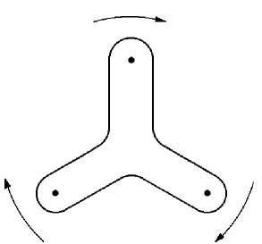
FIG. 1.:

FIG. 2.:

FIG. 3.:

FIG. 4.:

FIG. 5.:

REFERENCES

• [1] M. Casu and L.M. Sehgal, Phys. Rev. D55 (1997) 2644; Erratum ibid. D56 (1997) 3159
• [2] G. Karl, Phys. Rev. D45 (1992) 247
• [3] J. Bartelski and R. Rodenberg, Phys. Rev. D41 (1990) 2800
• [4] Ling-Fong Li and T.P. Cheng, Schladming Lectures, hep-ph/9709293 and references therein; T.P. Cheng and Ling-Fong Li, hep-ph/9709295; X. Song, hep-ph/9802206
• [5] L.M. Sehgal, Phys. Rev. D10 (1974) 1663; Erratum ibid. D11 (1975) 2016
• [6] J. Ellis and R.L. Jaffe., Phys. Rev. D9 (1974) 1444; Erratum ibid. D10 (1974) 1669
• [7] L.M. Sehgal, Proceedings of the EPS Int. Conf. on High Energy Physics, Geneva, 1979 (CERN Scientific Information Service, 1980) Vol.1, p.98; H. Yuta et al., Proceedings of the 12th Int. Conf. on Neutrino Physics and Astrophysics, Sendai, Japan, 1986, Eds. T. Kitagaki and H. Yuta (World Scientific 1986), p.525
• [8] M. Kawasaki, T. Maehara and M. Yonezawa, Phys. Rev. D57 (1998) 1822
• [9] T.T. Chou and C.N. Yang, Nucl. Phys. B107 (1976) 1
• [10] S. Brodsky, J. Ellis and M. Karliner, Phys. Lett. B206 (1988) 309
• [11] Hyun-Chul Kim, M. Polyakov, M. Praszalowicz, K. Goeke, Phys. Rev. D57 (1998) 299
• [12] D. Adams et al. (SMC Collaboration), Phys. Rev. D56 (1997) 5330; B. Adeva et al. (SMC Collaboration), Phys. Lett. B412 (1997) 414
• [13] K. Abe et al. (E143 Collaboration), hep-ph/9802357
• [14] G. Altarelli et al., Nucl. Phys. B496 (1997) 337 and hep-ph/9803237
• [15] M. Glück, R. Reya, M. Stratman and W. Vogelsang, Phys. Rev. D53 (1996) 4775; M. Stratman, hep-ph/9710379; T. Gehrmann and W.J. Stirling, Phys. Rev. D53 (1996) 6100; E. Leader, A.V. Sidorov and D.B. Stamenov, hep-ph/9708335
Figure Captions
• Fig.1.