Low-Energy Compton Scattering of
Polarized Photons on Polarized Nucleons
Abstract
The general structure of the cross section of scattering with polarized photon and/or nucleon in initial and/or final state is systematically described and exposed through invariant amplitudes. A low-energy expansion of the cross section up to and including the order is given which involves ten structure parameters of the nucleon (dipole, quadrupole, dispersion, and spin polarizabilities). Their physical meaning is discussed in detail.
Using fixed- dispersion relations, predictions for these parameters are obtained and compared with results of chiral perturbation theory. It is emphasized that Compton scattering experiments at large angles can fix the most uncertain of these structure parameters. Predictions for the cross section and double-polarization asymmetries are given and the convergence of the expansion is investigated. The feasibility of the experimental determination of some of the structure parameters is discussed.
pacs:
PACS: 11.80.Cr, 13.60.Fz, 13.88.+eI Introduction
Compton scattering on the proton at low and intermediate energies has thus far been studied mainly with unpolarized photons. Many recent data are available on the unpolarized differential cross section both in the region below pion threshold [1, 2, 3] and in the Delta region [4, 5, 6, 7, 8]. They have led to a determination of the dipole electric and magnetic polarizabilities of the proton, have given useful constraints on pion photoproduction amplitudes near the Delta peak, and have provided sensitive tests for different models of Compton scattering, such as those based on resonance saturation [9, 10, 11, 12], chiral perturbation theory [13, 14], and dispersion relations [15, 16, 17, 18, 19].
With the advent of new experimental tools such as highly-polarized photon beams, polarized targets, and recoil polarimetry [20], it becomes possible to study the very rich spin structure of Compton scattering. In particular, many additional structure parameters of the nucleon, such as the spin [21, 22, 23, 24] and quadrupole [25] polarizabilities, could be measured in such new-generation experiments and used for testing hadron models at low energies. The first attempt to determine the “backward” spin polarizability from unpolarized experiments has recently been reported [26]. Therefore, it is timely to give a detailed description of the appropriate polarization observables and their relationship to the low-energy parameters that might be measured in such experiments. That is the main purpose of the present report.
This paper is organized as follows. In Sect. II, we introduce the invariant Compton scattering amplitudes. In Sect. III we develop a general structure for the scattering cross section with polarized photons and/or polarized nucleons in the initial and/or final state. In Sect. IV we do a low-energy expansion of the invariant amplitudes and develop formulas for the low-energy expansion of the cross section and spin observables. In the process, we introduce and discuss the physical meaning of the parameters (polarizabilities) which are required to describe the cross section up to and including the order . In Sect. V we give theoretical predictions for all these polarizabilities by using fixed- dispersion relations and compare them with available predictions of chiral perturbation theory. We then investigate the range of validity of our low-energy expansion and show that it is generally valid below the pion threshold. Finally, we investigate quantitatively the dependence of different observables on the polarizabilities and recommend particularly sensitive experiments to perform. Some of the details related to the definitions and physical meaning of the polarizabilities are contained in the appendices.
II Invariant Amplitudes
The amplitude for Compton scattering on the nucleon,
| (1) |
is defined by
| (2) |
Constrainted by P and T-invariance, it can be expressed in terms of six invariant amplitudes as [27, 28, 15, 17, 18]
| (3) | |||||
| (4) |
where and are the photon polarization vectors, and are the bi-spinors of the nucleons (, is the nucleon mass), and . The orthogonal -vectors , , and are defined as
| (5) | |||||
| (6) |
where the antisymmetric tensor is fixed by the condition .
Unfortunately, there is no accepted standard for the definitions of the invariant amplitudes in nucleon Compton scattering. The definitions we use here may differ from those used in other works. We follow the conventions of Refs. [17, 18, 19], which are related to the so-called Hearn-Leader amplitudes used in Refs. [15, 28] by
| (7) | |||
| (8) |
The amplitudes are functions of the two variables and , where
| (9) |
are the usual Mandelstam variables and and . These functions have no kinematical singularities but they are subject to kinematical constraints arising from the vanishing of the denominators in the decomposition (3) in cases of forward or backward scattering. Therefore, it is useful to define the following linear combinations [18, 19, 29],
| (10) | |||||
| (11) | |||||
| (12) |
with
| (13) |
The amplitudes are even functions of , they have no kinematical singularities or constraints, and they have dimension .
In the Lab system (the nucleon at rest) the kinematic invariants , and read:
| (14) |
where , are the photon energies, is the photon scattering angle, and
| (15) |
We will reserve the symbols , , and for these Lab-frame variables. Note that in the Lab frame, , where is orthogonal to the reaction plane.
In terms of the , the Compton scattering amplitude in the Lab frame assumes the following form:
| (16) | |||||
| (17) | |||||
| (18) | |||||
| (19) | |||||
| (20) | |||||
| (21) | |||||
| (22) | |||||
| (23) |
where and the two magnetic vectors , are defined as:
| (24) |
III Cross sections and asymmetries
A General structure of the cross section
We will consider the general structure of the cross section and double-polarization observables in four related reactions:
| (26) | |||
| (27) | |||
| (28) | |||
| (29) |
We start by introducing the polarization variables.
Photon polarization properties are conveniently described in terms of the Stokes parameters () [30] which define the photon polarization matrix density as follows [31]:
| (30) |
Here the photon polarization vector is taken in the radiation gauge and denote either of two orthogonal directions which are in turn orthogonal to the photon momentum direction . Such a definition of is manifestly frame-dependent; nevertheless, the quantities
| (31) |
and are Lorentz invariant. They give the degree of linear and circular polarization, respectively. Moreover, corresponds to the right (left) helicity state, provided the -frame is right-handed. The total degree of photon polarization is given by . The values and separately are frame dependent, although they are still invariant with respect to boosts or rotations in the -plane. They define the angle that the electric field makes with the -plane:
| (32) |
To fix the azimuthal freedom in and , we first choose a frame in which all the momenta , , and are coplanar. This choice is not too restrictive and includes both the Lab and CM frames. In such a frame and for any polarized photon, either or , we take the -axis in (30) to lie along the direction of . Then the appropriate -axis is given by or , and the -axis is directed along or , respectively. The angle in (32) gives the angle between the electric field and the reaction plane. Thus defined, the Stokes parameters do not depend on further specification of the frame and are the same in the Lab or CM frame. We will use the prime to distinguish the Stokes parameters for initial or final photon, and .
Note that the above-defined Stokes parameters transform under parity as
| (33) |
under time inversion as
| (34) |
and under crossing as
| (35) |
The nucleon polarization matrix density is specified by a polarization 4-vector which is orthogonal to the nucleon 4-momentum [31]:
| (36) |
Introducing also the polarization 3-vector in the nucleon rest frame, one can relate and through the boost transformation,
| (37) |
where gives the degree of nucleon polarization. We apply the notations , and , for the initial and final nucleons, respectively.
Note that the vectors , are frame dependent and undergo Wigner rotation around the -axis when a boost in the reaction plane is applied. Nevertheless, is the same in the Lab and CM frame, although that is not the case for .
In both the Lab and CM frames, the differential cross section of the reactions (III A) reads:
| (38) |
Here the square of the Lorentz-invariant matrix element , appropriately averaged and summed over polarizations, has the same generic form in all four cases (III A),
| (39) |
where we set , and for the moment we disregard optional primes distinguishing polarization variables for initial and final particles. Since and are axial vectors and , have odd P-parity, some of the invariant functions must vanish:
| (40) |
In terms of the remaining , the generic expression (39) gets the following specific form for the individual cases given in Eq. (III A):
| (43) | |||||
| (45) | |||||
| (47) | |||||
| (49) | |||||
Note that the same functions determine the cross section in Eqs. (43) and (49) (as well as in Eqs. (45) and (47)) which are related through T-invariance; the negative signs in (45), (49) are easily found from Eq. (34). The relationship between the cases (43) and (45) is determined by the crossing symmetry of the amplitude and Eq. (35):
| (50) | |||||
| (51) | |||||
| (52) | |||||
| (53) |
In terms of the invariant amplitudes or , the functions read (cf. Ref. [32]):
| (56) | |||||
| (59) | |||||
| (61) | |||||
| (62) | |||||
| (63) | |||||
| (64) | |||||
| (65) | |||||
| (67) | |||||
| (68) | |||||
| (70) | |||||
| (71) | |||||
| (73) | |||||
| (75) | |||||
| (77) | |||||
| (79) | |||||
| (80) |
Below the pion photoproduction threshold, the amplitudes , are real, and therefore only the six structures, and , are different from zero.
B Asymmetries
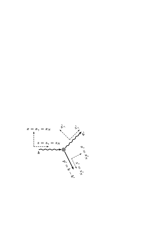
The thirteen invariant quantities standing in Eq. (40) intervene directly in the definition of polarization observables which can be measured experimentally. Not all of them are independent, since with 6 complex invariant amplitudes there are only 11 independent observables. In the following we shall classify them according to the number of polarization degrees of freedom involved in the process. We shall define some -index asymmetries , and , where or refers to the photon Stokes parameters or , and or refers to the right-handed axes along which the nucleon spin or may be aligned. At this point we have to relate the products like , , and in Eq. (40) to the spin vector (or ), and eventually fix a frame. We choose the Lab frame for practical reasons; for any other frame only the coefficients introduced below have to be recalculated. We will indicate all necessary changes to be done for the CM frame.
Directing the and axes along , we choose the -axis along the photon beam direction . Note that since , all the asymmetries obtained in this way in the Lab frame for the reactions (III A-a,b) with the polarized nucleon are the same in the CM frame. In the case of the polarized final nucleon, we choose the axis to lie along the nucleon recoil momentum . Such an axis depends on whether we use the Lab or CM frame so that we get different, though related, asymmetries.
We can further simplify the notation. The axes and are identical and we will denote them in the following by simply . For we will use . Note that, despite the fact that the - and -axes are the same, we will keep the prime when using because it identifies which nucleon ( or ) we are referring to. All these axes are shown in Fig. 1.
The set of observables is defined as follows.
Polarization-Independent Observable (), or simply the unpolarized cross section,
| (81) |
Single-Polarization Observables (), of which there are two for each of the reactions (III A):
(i) the beam asymmetry for photons which are linearly polarized either parallel or perpendicular to the scattering plane and unpolarized nucleons (target and recoil). The same quantity gives the degree of linear polarization () of the photon scattered from unpolarized nucleons:
| (82) |
(the primed polarizations or refer to the final photon state). This asymmetry is often designated as .
(ii) the target asymmetry or recoil polarization for unpolarized photons, whereby either or is polarized along the directions:
| (83) |
Here the coefficient
| (84) |
(as given through both Lab and invariant quantities) determines the scalar product . It is just the negative--component of . The asymmetry is often designated as , the recoil nucleon polarization.
Double-Polarization Observables (), of which there are five for each of the reactions (III A):
(i) the beam-target asymmetry for incoming linearly polarized photons, either parallel or perpendicular to the scattering plane , and target nucleon polarized perpendicular to the scattering plane. The same quantity can be measured as the correlation of polarizations of the outgoing particles and :
| (85) | |||||
| (86) |
Another independent quantity is the correlation of the beam polarization and the polarization of recoil nucleon, or the correlation of the target polarization with the final photon polarization:
| (87) | |||||
| (88) |
(ii) the asymmetries with circular photon
polarizations .
The general expression for the asymmetry with circularly polarized photons
follows from Eq. (40). For example, for the reaction
(III Aa)
| (89) |
Such a quantity survives when the nucleon spin lies in the reaction plane. Considering the cases with the target spin aligned in or directions, we can introduce the beam-target asymmetries
| (90) | |||
| (91) |
and the scattered photon-target asymmetries
| (92) | |||
| (93) |
Here the coefficients determine the scalar products
| (94) |
In terms of Lab or invariant quantities, they read
| (95) | |||
| (96) | |||
| (97) |
Numerically, are the same in the Lab and CM frames.
Another four asymmetries, which are depend linearly on those in Eqs. (90)-(92), describe the correlations of the recoil polarization with the polarization of the photons or :
| (98) | |||
| (99) | |||
| (100) | |||
| (101) |
They are given by the coefficients appearing in the expansions
| (102) |
which in the Lab frame read
| (103) |
where . Since the -axis in the CM frame is different from that in the Lab frame, the corresponding are different too. Except for the signs, they coincide with in Eq. (95):
| (104) |
(iii) the asymmetries with photons linearly polarized at with respect to the scattering plane (. For example, in the case (III Aa),
| (105) |
With the same considerations discussed for Eq. (90), one can define the asymmetries
| (106) | |||
| (107) | |||
| (108) | |||
| (109) |
and a similar linearly dependent set
| (110) | |||
| (111) | |||
| (112) | |||
| (113) |
One can get another representation (with , etc.) for the above asymmetries by using the following relations among the cross sections that have opposite in-plane nucleon (target or recoil) polarizations:
| (114) |
and similarly for the primed cross sections (with the polarized final photon). These relations are due to parity conservation.
Introducing the generic quantities
| (115) | |||||
| (116) | |||||
| (117) |
one can write the differential cross section in the following compact form:
| (118) |
which, being supplied with appropriated primes, is valid for any combination of ingoing or outgoing polarized particles.
Thus, with unpolarized and linearly polarized initial or final photons, one can access two observables: and , respectively. When the nucleon (target or recoil) polarization is added, four more asymmetries appear, and , , (and their primed companions), all of which vanish below the pion threshold. When circularly polarized photons are used with polarized nucleons, two more asymmetries appear, and , both of which survive below the pion threshold.
It is important to emphasize that the formulas like (38) and (118), being used for polarized particle(s) in the final state, give the total yield of the particles and their polarization matrix density. To get a partial cross section of a particle produced with specific final polarization(s), one must use an average instead of a sum over polarizations. That is equivalent to inserting the statistical factor into these formulas, where for the cases (III A-a,b,c,d), respectively.
IV Low-energy expansions
A Invariant amplitudes and polarizabilities
A very general method for obtaining low-energy expansions of physical amplitudes for different reactions consists in introducing invariant amplitudes free from kinematical singularities and constraints and expanding them in a power series [33, 34]. Following this method, we first decompose the invariant amplitudes into Born and non-Born contributions,
| (119) |
The Born contribution is associated with pole diagrams involving a single nucleon exchanged in - or -channels and vertices taken in the on-shell regime,
| (120) |
It is completely specified by the mass , the electric charge , and the anomalous magnetic moment of the nucleon:
| (121) |
where is the elementary charge, , and for the proton and neutron, respectively. The pole residues read
| (122) | |||
| (123) |
The Born contribution to possesses all the symmetries of the total amplitude , including gauge invariance, and takes all singularities of at low energies.
The non-Born parts of the invariant amplitudes, which contain all the structure-dependent information, are regular functions of and and can be expanded as a power series in and . Since
| (124) |
such an expansion can be recast as a power series in the cross-even parameter :
| (125) |
Here the low-energy constants
| (126) |
parametrize the structure of the nucleon as seen in its two-photon interactions.
The expansion (125) directly leads to a corresponding low-energy expansion of the total amplitude in the Lab frame. We first consider the spin-independent part of Eq. (16). The spin-independent part of the Born term follows from Eq. (16):
| (128) | |||||
Here . The leading term in (128) reproduces the Thomson limit,
| (129) |
The non-Born contribution to is determined by the structure constants introduced in the expansion (125). Its spin-independent part starts with a term,
| (130) |
Here the constants and ,
| (131) |
are identified as the dipole electric and magnetic polarizabilities of the nucleon, just in accordance with an effective dipole interaction
| (132) |
of the nucleon with external electric and magnetic fields, leading to the amplitude (130). Due to its interference with the Thomson amplitude (129), the contribution of the polarizabilities, Eq. (130), results in a effect in the differential cross section in the case of the proton () and in a effect in the case of the neutron ().
The terms in Eq. (130) are also easily read out from Eqs. (16) and (125). They are determined by the dipole polarizabilities and the following combinations of - and -derivative constants and of the amplitudes , and :
| (133) | |||||
| (134) | |||||
| (135) | |||||
| (136) |
These polarizability-like quantities are constant coefficients of energy- and angle-dependent corrections to the dipole interaction (132) which enter to next order in photon energy. The recoil correction in Eqs. (133) is explained in Appendix C.
We now introduce linear combinations of the parameters (133) which have a more direct physical meaning. If we consider the partial-wave structure of the amplitude (see Appendix A), we can relate the -derivative constants in Eq. (133) to the quadrupole polarizabilites of the nucleon [25]:
| (137) |
A nonrelativistic example is given in Appendix B. The quantities
| (138) |
which we call “dispersion polarizabilities”, describe the -dependence of the dynamic dipole polarizabilities. In terms of the parameters , , , and , the corresponding effective interaction of has the form
| (139) |
where the dots mean a time derivative and
| (140) |
are the quadrupole strengths of the electric and magnetic fields.
We next consider the spin-dependent part of Eq. (16). The spin-dependent part of starts with terms which come from the Born contribution. To leading order one has [35],
| (142) | |||||
The omitted higher-order terms can be read out from Eqs. (16) and (121).
As shown in Eq. (16), the non-Born part of starts with terms. They are determined by the four constants , , , and . Due to their interference with the spin-dependent terms of Eq. (142), they give rise to a correction to the unpolarized cross section. In the case of a polarized proton and a circularly polarized photon, these terms appear at the order .
The terms in were considered in several papers [21, 22, 23]. In the most recent (and best known) work [23] they are parametrized as
| (146) | |||||
where are structure parameters (often called the “spin polarizabilities”) which are linear combinations of the constants (see Appendix A). In the following we consider a linear combination of these parameters
| (147) | |||||
| (148) | |||||
| (149) | |||||
| (150) |
which have a more transparent physical meaning, as explained in Appendices A and B. The parameters and describe the spin dependence of the dipole electric and magnetic photon scattering, and , whereas and describe the dipole-quadrupole amplitudes and , respectively. The amplitude (146) implies an effective spin-dependent interaction of order
| (151) |
To summarize, we have obtained a low-energy expansion of the amplitudes for nucleon Compton scattering. To , the cross section and polarization observables are determined by 10 polarizability parameters:
-
Two dipole polarizabilities: and
-
Two dispersion corrections to the dipole polarizabilities: and
-
Two quadrupole polarizabilities: and
-
Four spin polarizabilities: , , ,
These polarizabilities have a simple physical interpretation in terms of the interaction of the nucleon with an external electromagnetic field. Equivalently, these ten parameters are linear combinations of the low-energy constants, Eq. (126), representing the zero-energy limit of the six invariant amplitudes plus two combinations of both the - and -devivatives of these amplitudes.
To illustrate the interplay among all these polarizabilities, we consider the two limiting cases of forward and backward scattering.
(i) The amplitude for forward scattering,
| (152) |
has the following low-energy decomposition:
| (154) | |||||
where
| (155) |
is the “forward-angle spin polarizability”, and
| (156) |
(ii) The amplitude for backward scattering,
| (158) | |||||
has the following low-energy decomposition:
| (161) | |||||
where
| (162) |
is the “backward-angle spin polarizability”, and
| (163) |
B Cross sections
A decomposition analogous to (119) can be applied also to the invariant functions :
| (164) |
The Born contribution is given by
| (167) | |||||
| (168) | |||||
| (170) | |||||
| (172) | |||||
The non-Born contributions are more conveniently written by separating the terms of different order in . In particular, for and we have
| (173) |
where
| (175) | |||||
| (176) | |||||
| (179) | |||||
| (181) | |||||
Here and are polynomials in of the third and zero order, respectively, which are determined by the spin polarizabilities as follows:
| (182) | |||||
| (183) | |||||
| (184) | |||||
| (185) |
and
| (186) |
For the invariants and we can stop the expansion at , since they appear in the squared amplitude multiplied by terms of . Therefore we have
| (187) |
where
| (190) | |||||
| (192) | |||||
| (194) | |||||
| (197) | |||||
In order to illustrate the interplay between polarizabilities and the cross sections (in the Lab frame), we consider below the case of polarized photon beam and polarized target at , , and .
(iii) At :
| (207) | |||||
| (210) | |||||
| (213) | |||||
| (216) | |||||
For the low-energy expansion of the amplitudes and structure functions, two further remarks must be considered. First, as is evident from Eq. (3), the -channel -exchange contributes only to (and thus only to ). Owing to the small pion mass , this diagram is a rapidly varying function of and therefore it is profitable to keep its expression unexpanded. This can be achieved with the following replacement in the non-Born part of the amplitude :
| (217) |
where
| (218) |
with or for the proton and neutron, respectively, and where
| (219) |
is the two-photon decay width. The relative sign of the coupling and the coupling is negative. In Eq. (217), is a smoother function of than and is better approximated by a polynomial in (which is just the constant to the order we consider). In terms of the spin polarizabilities, this means that the following substitutions have to be done in all the expansions:
| (220) | |||||
| (221) |
where
| (222) |
Generally, after the separation of the -exchange contribution, all the low-energy expansions discussed in this section become valid provided is a small parameter. The radius of convergence of the -series is, up to a small correction of order , equal to
| (223) |
and is determined by the pion photo-production threshold where the amplitudes have a singularity and acquire an imaginary part. Another close singularity is due to the -channel exchange of two pions, which gives the same restriction (223).
The second remark is that the low-energy expansions of the structure functions , when used within the radius of convergence, give an accurate account of the dependence of the cross sections on the dipole polarizabilities , and the spin polarizabilities , , , . In the expressions for and , the spin polarizabilities enter to leading order as an interference with the Thomson amplitude (129). The subleading terms of order appear due to interference with the amplitude (142). Numerically the latter terms are enhanced by the anomalous magnetic moment (for example, in Eq. (161) for the proton) and are as important as the leading terms. On the other hand, in the expansions for , the leading order contribution of the quadrupole and dispersion polarizabilities , , , are already of order , which is the highest order included in the expansion. Therefore the subleading terms which describe the interference of these polarizabilities with the amplitude (142) are not included, although they may be comparable in magnitude to the leading terms. For this reason, it is generally more accurate to use low-energy expansions for the invariant amplitudes , including all ten polarizabilities which appear to the order considered, and then to calculate the structure functions through Eqs. (III A). This more accurate technique will be used when we discuss the low-energy observables in Section V.
In principle, all the polarizabilities we have defined can be determined from experiment. For example, in the proton case once the dipole polarizabilities and have been determined (from low-energy experiments that are sensitive only to terms of order ), the angular behavior of the coefficients and (from the measurements of and ) enables a determination of all the spin polarizabilities , , , . Then the angular dependence of the unpolarized cross section allows one to determine the remaining polarizabilities , , , . In the next section, we investigate the feasibility of this approach.
V Discussion
In this section we summarize some theoretical predictions for the polarizabilities, examine the question of convergence of the low-energy expansion, and discuss the sensitivity of various observables to these polarizabilities.
A Theoretical predictions for polarizabilities
We now consider various theoretical predictions for the polarizabilities in order to establish the accuracy which should be achieved in experiments to make them useful for resolving theoretical ambiguities. We restrict ourselves to estimates based on chiral perturbation theory and dispersion relations, since these have proved to be successful in applications to strong and electromagnetic interactions of hadrons at low energies.
In its standard form, chiral perturbation theory gives leading-order (LO) predictions for the polarizabilities entirely in terms of the pion mass , the axial coupling constant of the nucleon, , and the pion decay constant MeV. The nucleon mass which describes recoil corrections does not enter into the LO predictions but appears in the next-to-leading order together with some additional parameters. The LO-contributions dominate in the chiral limit and are expected to provide semi-quantitative estimates in the real world. All results quoted here were obtained by Bernard et al., as summarized in Ref. [13]. Using explicit formulas from that work, we have
| (224) | |||
| (225) | |||
| (226) | |||
| (227) | |||
| (228) |
Here the quantities are proportional to -th powers of the inverse pion mass:
| (229) | |||
| (230) |
where is the threshold photoproduction amplitude for charged pions in the chiral limit. Since the values , , are determined by pion loops with charged pions, we use the charged pion mass MeV for obtaining numbers for these ’s. The terms with describe the exchange (218) with couplings fixed by the chiral anomaly (Wess-Zumino-Witten) and by the Goldberger-Treiman relation:
| (231) |
Accordingly, we use the neutral pion mass MeV to evaluate .111In principle, the difference between the masses of and runs beyond the accuracy of leading-order predictions. Its consistent treatment has to involve radiative corrections of . However, we assume that the use of the experimental masses of the pions in the present context still makes sense because this is expected to reduce the size of the counter-term contributions which come from the full treatment.
Calculation to the next order(s) involves new parameters (counter-terms) which are usually estimated via an approximation that takes into account the nearest resonances and/or loops with strange particles. Such a procedure may lead to rather different results for polarizabilities, depending on further details (for example, compare Ref. [13] and Ref. [14]; see also below). Among the nucleon resonances, the is special because it is separated from the nucleon by a relatively small energy gap and has a large coupling to the channel. Therefore this resonance is particularly important for low-energy phenomena such as the polarizabilities. In Refs. [14, 36], the was considered as a partner of the nucleon in the chiral expansion, which was reformulated in terms of a generic small energy scale . In the following we invoke only one component of such an approach, the -pole contribution. We ignore the contribution of pion loops with an intermediate . These terms are relatively small for the spin polarizabilities, although large for and . We take into account both and couplings of the . Although the quadrupole contribution is of higher order in , numerically it is not negligible for the spin polarizability . For the -pole contribution we have
| (232) | |||
| (233) |
(and nothing for the other polarizabilities, as discussed in detail in Appendix D). Here and are the magnetic and quadrupole transition moments, respectively. Depending on how the -coupling is extracted from the experimental radiative width of the (with relativistic or nonrelativistic phase space), the -pole contribution to was evaluated in [14, 36] as
| (234) |
(units are ).222This difference also illustrates how estimates of counter-terms may depend on assumptions. With the generally accepted phenomenological magnitude of (see, for example, [37]), [29, 38]. In the Skyrme model [39] or large- QCD [40], the transition magnetic moment is related to the isovector magnetic moment of the nucleon as , so that . All these contributions are summarized in Table I, where the larger magnitude of Eq. (234) has been assumed. With the fixed ratio fm (see Appendix D), the use of the other value would reduce all the -pole contributions by 40%.
Another way to calculate the polarizabilities is provided by dispersion relations for the amplitudes . In the following we give results of the fixed- dispersion relations which have the form [19]
| (235) |
Here the dispersion integral is taken from the pion photoproduction threshold to some large energy (actually, it is 1.5 GeV). The remaining so-called asymptotic contribution is -dependent but only weakly energy dependent. From unitarity, the imaginary part of the amplitudes and the integral in Eq. (235) can be calculated by using experimental information on single- and double-pion photoproduction which is available at energies below . In the present context we use the latest version of the single-pion photoproduction amplitudes provided by the partial wave analysis of the VPI group [41] (the code SAID, solution SP97K). Also, double-pion photoproduction is taken into account in the framework of a model which includes both resonance mechanisms and nonresonant production of the and states. Details of this procedure are given in Ref. [19].
The quantities take into account contributions of high energies into the dispersion relations. According to Regge phenomenology, only the amplitudes and can have a nonvanishing part at high energies and thus have a large asymptotic contribution. For the other amplitudes (), the dispersion integrals provide a very good estimate of the corresponding non-Born parts. Thus, we can reliably find through Eq. (235) the constants and , , , . Moreover, the constant can be found as well, since it is not affected by the asymptotic contribution. Uncertainties appear only for the constants , , and , which get a sizable contribution from the asymptotic part of the amplitude.
Following the arguments of Ref. [19], we relate the asymptotic contributions to the -channel exchange of the and mesons, respectively. The couplings of the are well known, and we include this contribution by virtue of Eq. (218), in which we use experimental values for couplings and introduce a monopole form factor with MeV. The experimental magnitude of the product is higher than that given by the anomaly equation (231). However, the form factor reduces the strength by and makes the resulting contribution at very close to that given by the anomaly (see Table I). Nevertheless, beyond the , the amplitude can have contributions from other heavier exchanges and thus have an additional piece which weakly depends on . 333 A recent analysis [26] of unpolarized Compton scattering data suggests the existence of such an additional contribution, since the spin polarizability found there deviates considerably from that predicted by the dispersion integral (235) for the amplitude and by the asymptotic contribution (see Table I). Even after allowing for an uncertainty of in the integral contribution given in Table I, as suggested by a sizable integrand at energies above 1 GeV where calculations of are very model dependent, such a strong deviation is difficult to understand theoretically and needs to be confirmed by additional experimental measurements. Therefore the fixed- dispersion relation for should not be considered as a reliable source of information on .
The amplitude gets a large asymptotic contribution from exchange, which contributes to the constant and therefore to the difference of the dipole polarizabilities . Since this difference is experimentally known for the proton to be [3], as determined by low-energy Compton scattering data, the constant is known too. However, the quantity is not fixed by these data and cannot be unambiguously predicted from the dispersion relations (235). Using data on scattering at higher energies (above 400 MeV), the -dependence of the asymptotic contribution at was estimated in [19]. It corresponds to a monopole form factor with the cut-off parameter MeV (“mass” of the ). However, the -dependence of at smaller might be somewhat steeper as suggested from independent estimates. Therefore, the fixed- dispersion relation for should not be considered as a reliable source of information on .
With these precautions, we put into Table I the results of saturating the dispersion integrals by known photoproduction amplitudes and by the asymptotic contributions discussed above. We assume that is the same for the proton and neutron. Depending on which photoproduction input is used, the integrals are slightly different. We give both our results, which use the SAID solution SP97K as an input and a model for double-pion photoproduction, and the results by Drechsel et al. [42], which use photoproduction amplitudes by Hanstein et al. (HDT) [43] (and ignore the double-pion channel). The main difference between these two evaluations comes from near-threshold energies where the SAID and HDT multipoles are rather different (see Ref. [42] for details). For some other (generally similar) dispersion estimates, see Refs. [22, 47, 48]. Available experimental data are also given in the footnotes to Table I, including measurements of and for the proton (see Ref. [3] and references therein), measurements of for the neutron [44, 45] (see also [46] for critical discussion), and a recent estimate of for the proton [26]. It is apparent from Table I that it is necessary to measure the spin polarizabilities to an accuracy in order to obtain constraints valuable for the theory.
Similarly to Ref. [42], we can isolate quantities which can be reliably predicted by the dispersion relations (235) (up to small uncertainties coming from the photoproduction amplitudes), namely those which do not depend on , , and (see Table II). In the absence of precise data on double-polarized Compton scattering at low energies, these predictions can be used to diminish the number of unknown parameters during fits and to help in determination of unconstrained combinations. These latter combinations are (which has already been measured), , and . Therefore, the most interesting and informative experiments on Compton scattering are those which are sensitive to the parameters and , which mainly contribute to the backward scattering amplitude. Below we discuss which observables are the best suitable to this aim. The above remarks apply principally to the proton. The case of the neutron can considered in a similar manner. However, since a free neutron target is not available, neutron polarizabilities are studied through elastic or inelastic nuclear Compton scattering, thereby introducing additional uncertainites due to Fermi motion, meson exchange currents, final-state interactions, etc. (see, e.g., Refs. [49, 50]).
B Convergence of the low-energy expansion
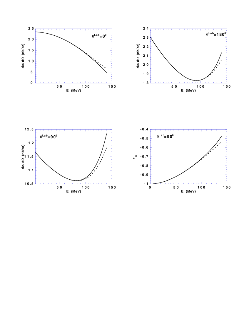
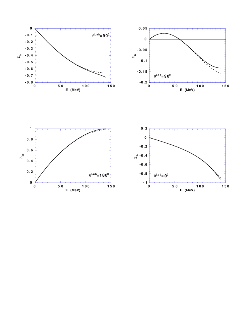
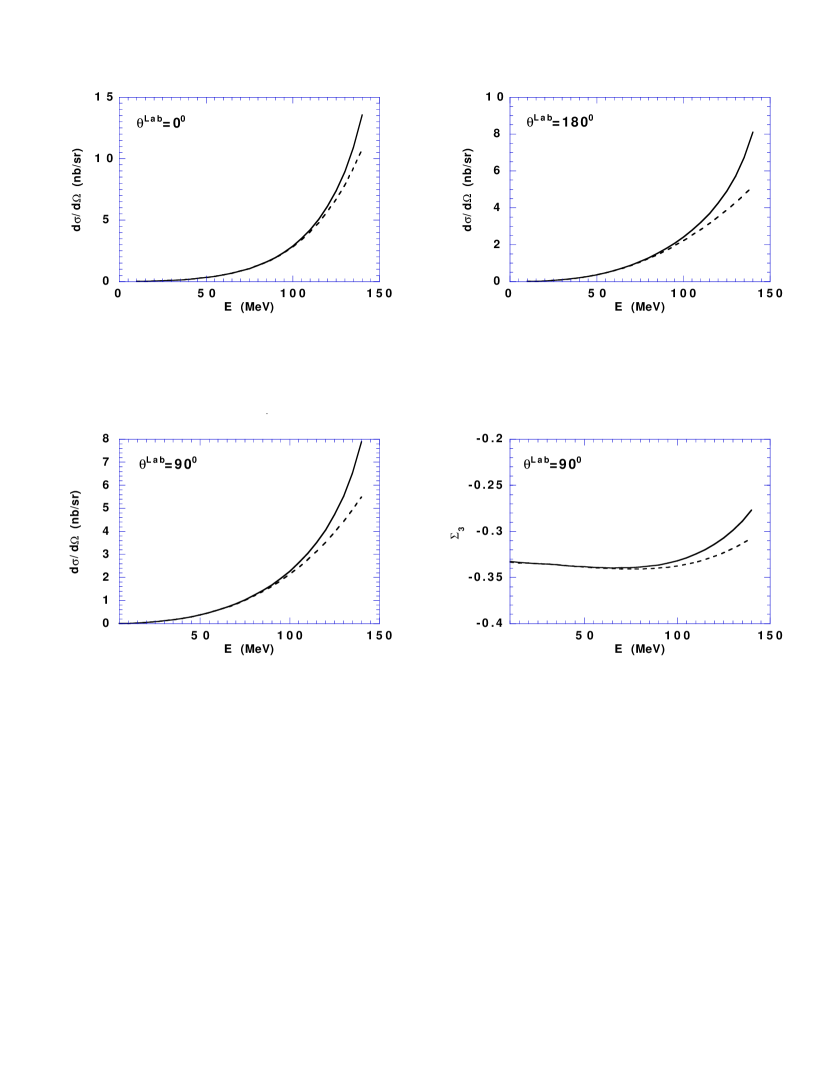
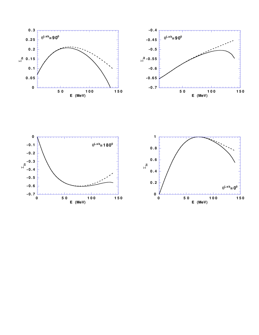
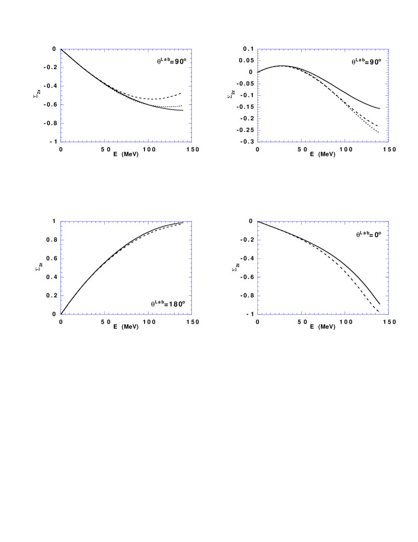
In order to investigate the convergence of the low-energy expansion, we use the same fixed- dispersion relations described in the preceeding section to make an exact prediction for the invariant amplitudes at any energy. From these the can be calculated exactly and predictions for the various observables can be made. These can be compared with predictions calculated by truncating the to , as described in Section IV. Such a comparison is shown in Figs. 2 and 3 for the proton and Figs. 4 and 5 for the neutron. For the proton, the expansion works very well for energies up to the pion threshold. For the neutron, it appears to work less well due to the fact that the Born contributions are considerably smaller than for the proton. The full calculation deviates rapidly from the expansion once the pion threshold is crossed.
C Sensitivity of observables to polarizabilities
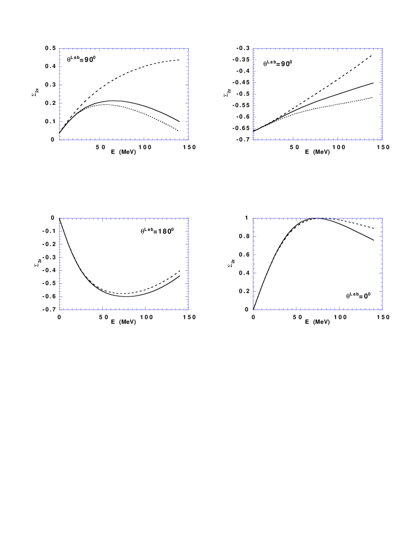
We now address the question of the measurement of the polarizabilities we have defined, with the principal focus being on the spin polarizabilities. To the order of our expansion, the double polarization observables are not sensitive to the quadrupole and dispersion polarizabilities, whereas the unpolarized cross section and are sensitive to all of the polarizabilities. Therefore it seems reasonable to use double polarization measurements to constrain the , then unpolarized measurements to measure the remaining polarizabilities. At extreme forward and backward angles, the observable is sensitive to the in the combinations that give (Eq. 155) and (Eq. 162), respectively. Two other linear combinations can be obtained from measurements of and at 90∘. Indeed, the formulas given at the end of Section IV suggest that these measurements are primarily sensitive to and , respectively, at least to the lowest order. In Figs. 6 and 7 we show these observables as a function of energy, as calculated using our low-energy expansion with polarizabilities fixed by the SAID dispersion relation values given in Table I. In order to evaluate the sensitivity of the observable to the polarizability, we have adjusted various quantities by fm4 relative to the value in Table I. This amount is comparable to the pion loop contribution to each of the polarizabilities but is somewhat larger than the typical discrepancy among the competing theories.
We conclude that in the energy regime below pion threshold where the low-energy expansion is valid, it will be very difficult to measure the spin polarizabilities to an accuracy that can discriminate among the theories, at least at the extreme forward and backward angles. In particular, the backward spin asymmetry is almost completely insensitive to theoretically motivated changes to , whereas the forward spin asymmetry is only moderately sensitive to changes in . Somewhat more sensitive are the asymmetries at 90∘, which might provide some useful constraints on and . Most promising is for the neutron, which is remarkably sensitive to changes in .
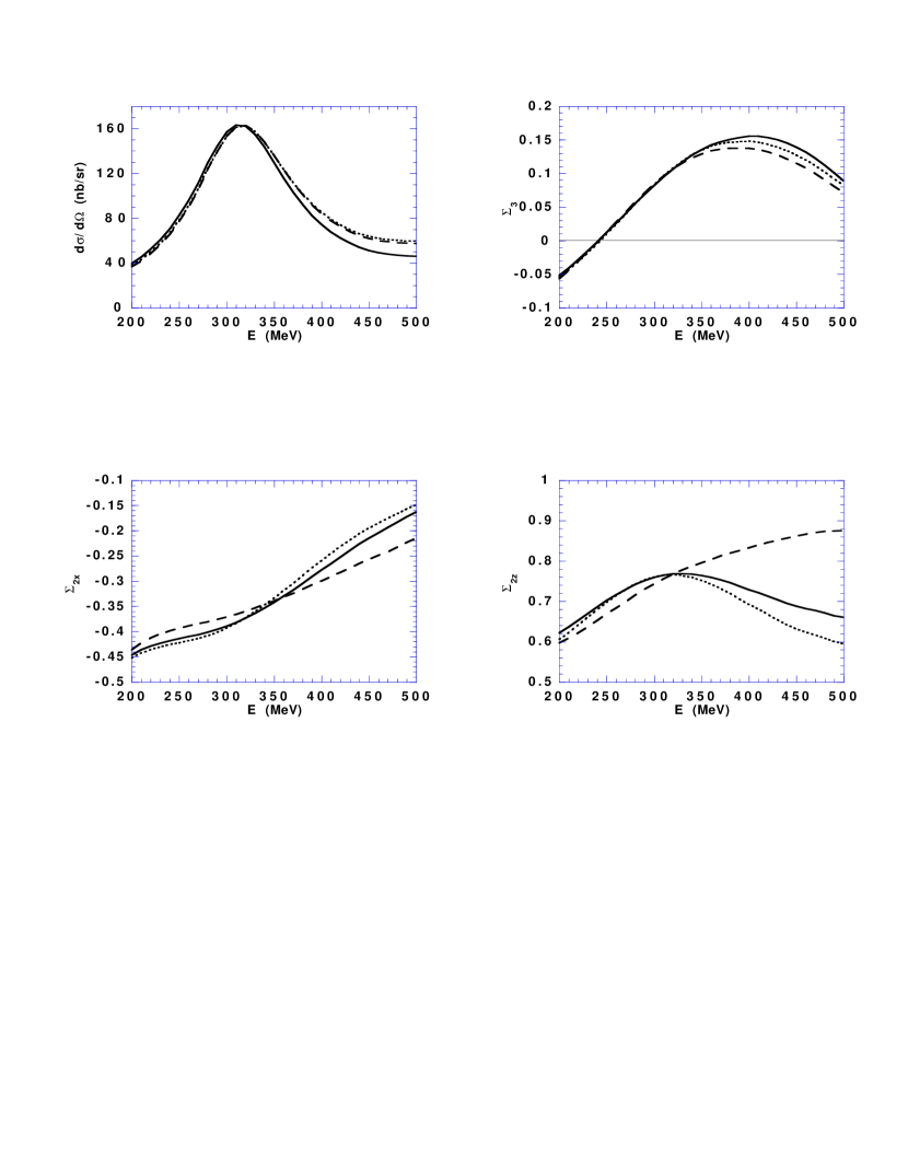
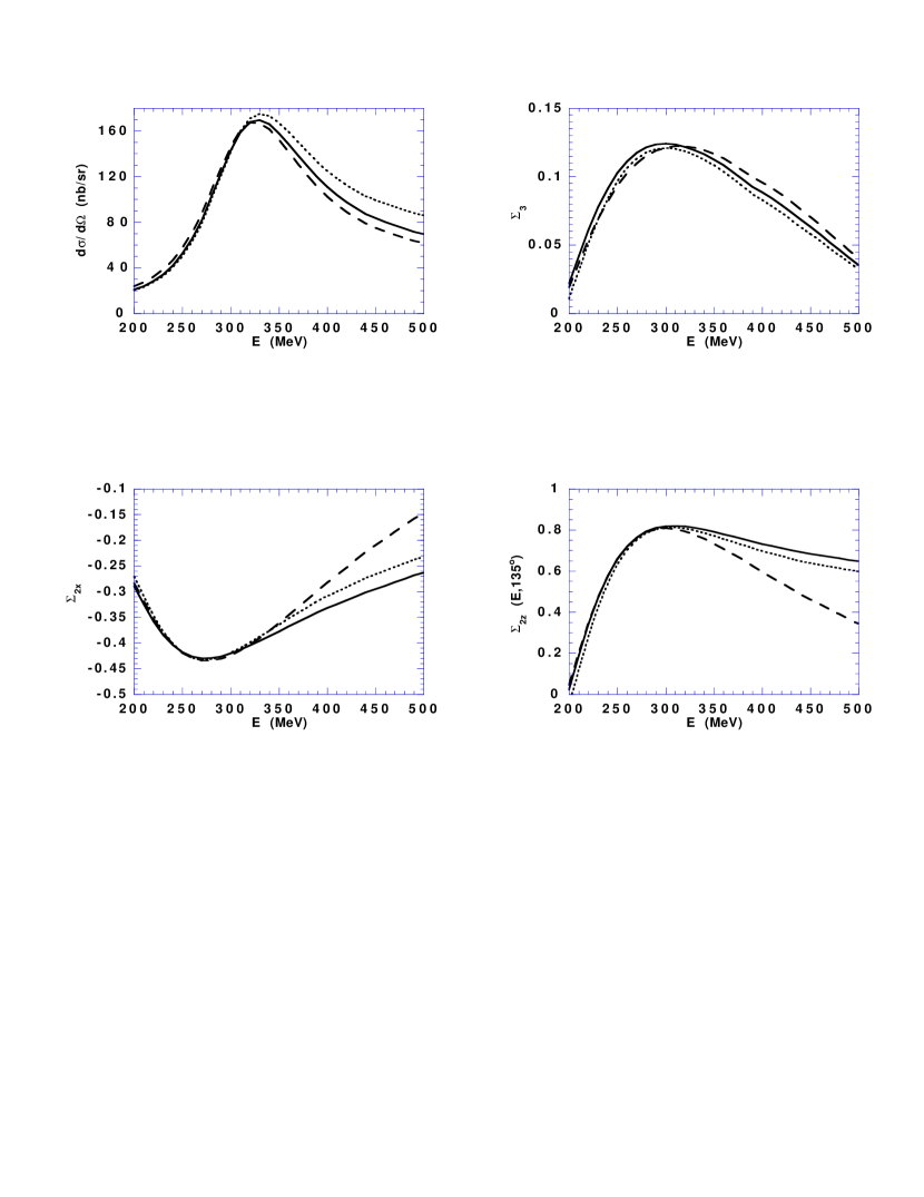
At higher energy, the spin asymmetries are more sensitive to the spin polarizabilities, but of course the low-energy expansion is no longer valid. Dispersion theory provides a convenient formalism for interpreting Compton scattering data beyond the low-energy approximation, but only for those polarizabilties not already constrained by the same dispersion relations. As discussed above, and are not well constrained by the dispersion relations due to potentially unknown asymptotic contributions to and , respectively. We therefore investigate whether Compton scattering in the so-called dip region between the and higher resonances might usefully constrain these two parameters. In Figs. 8 and 9 we present calculations of the unpolarized cross section and the spin observables , , and in the energy range 200–500 MeV. In these calculations, the parameter was adjusted by changing the mass in the asymptotic contribution , where was already fixed by experimental data on . The parameter was adjusted by adding to the asymptotic contribution from the -exchange a contribution of heavier exchanges, i.e. by using in the dispersion relations the ansatz , where was an adjusted constant and was a monopole form factor with the cut-off parameter MeV. In the unpolarized cross section for the proton, a change of from to is indistinguishable from a change in the mass from 500 to 700 MeV (which changes from 49 to 38). However, these possibilities are easily distinguished with , so that a combination of unpolarized and polarized measurements in this energy range offers the possibility of placing strong constraints on both and . Of course, any practical determination of the polarizabilites from Compton scattering data at energies of a few hundred MeV has to take into account uncertainties in the photopion multipoles used to evaluate the dispersion integrals. At the moment, these uncertainties are not negligible (see Ref. [26]).
VI Summary
The general structure of the Compton scattering amplitude from the nucleon with polarized photons and/or polarized nucleons in the initial and/or final state has been developed. A low-energy expansion of the amplitude to has been given in terms of ten polarizabilities: two dipole polarizabilities and , two dispersion corrections to the dipole polarizabilities and , two quadrupole polarizabilities and , and four spin polarizabilities , , , and . The physical significance of the parameters has been discussed, and the relationship between these and the cross section and spin observables below the pion threshold has been established. We have also presented theoretical predictions of these parameters based both on fixed- dispersion relations and chiral perturbation theory. We have established that the range of validity of our expansion extends to the pion threshold. We have shown that low-energy experiments will have to be very precise to resolve the theoretical ambiguities in the polarizabilities. However, we have suggested that measurements at higher energy might help fix the most theoretically uncertain of them, particulary the backward spin polarizabilitiy and the difference of quadrupole polarizabilities .
Acknowledgements.
A.L. appreciates the hospitality of the University of Illinois at Urbana-Champaign and the Institut fur Kernphysik at Mainz where a part of this work was carried out. This work was supported in part by the National Science Foundation under Grant No. 94-20787.A Multipole content of polarizabilities
1 Centre-of-mass amplitudes
In the CM frame, the amplitude of nucleon Compton scattering can be represented by six functions of the energy and the CM angle as [51, 53]
| (A1) |
where and the spin basis reads
| (A2) | |||
| (A3) |
In the particular cases of forward or backward scattering,
| (A4) | |||||
| (A5) |
Some authors [28, 23, 13, 36] utilize a different spin basis, and the following identities provide links with the notation of those works:
| (A6) | |||||
| (A7) | |||||
| (A8) |
where and where we have used .444 A few other relations can be obtained from (A6) by doing a dual transformation, , (and the same for primed vectors) which is just a -rotation of the polarizations. Under such a transformation, , , and . In particular, the amplitudes from [36] (we denote them here by ) read
| (A9) | |||
| (A10) |
where .
The CM amplitudes are related to the invariant amplitudes (10) by
| (A11) | |||||
| (A12) | |||||
| (A13) | |||||
| (A14) | |||||
| (A16) | |||||
| (A18) | |||||
Here and
| (A19) | |||
| (A20) |
Note also that the invariants , , are
| (A21) |
In the important case of low energies (or very heavy nucleon), one has
| (A22) | |||||
| (A23) | |||||
| (A24) |
up to higher orders in . Here and .
A multipole expansion of the amplitudes has the form [52, 53, 54]
| (A25) | |||||
| (A26) | |||||
| (A27) | |||||
| (A28) | |||||
| (A30) | |||||
| (A32) | |||||
Here are Legendre polynomials of . The multipole amplitudes with correspond to transitions and the superscript indicates the angular momentum of the initial photon and the total angular momentum . Due to T-invariance,
| (A33) |
Keeping only dipole-dipole and dipole-quadrupole transitions in these formulas, we obtain
| (A34) | |||
| (A35) | |||
| (A36) |
(plus higher multipoles, which introduce an angular dependence to the amplitudes ).
2 Polarizabilities to order
Low-energy expansions of the amplitudes are obtained from (A11) and (125) [22]. Leading nonvanishing terms of are given by the Born term, in accordance with the low-energy theorem by Gell-Mann-Goldberger-Low:
| (A37) | |||
| (A38) | |||
| (A39) |
where and is the electric charge of the nucleon. Structure-dependent (i.e. non-Born) contributions to start with the terms
| (A40) | |||||
| (A41) | |||||
| (A42) |
where coefficients are directly read out from Eq. (A22):
| (A43) | |||||
| (A44) | |||||
| (A45) |
Here the constants are those that appeared in Eq. (146).
The physical meaning of these polarizabilities can be understood by using the multipole expansion (A34). Comparing with Eq. (A40), we identify the polarizabilities as leading terms in the structure-dependent multipoles:
| (A46) | |||||
| (A47) | |||||
| (A48) | |||||
| (A49) | |||||
| (A50) | |||||
| (A51) |
It is seen that some of these describe mixed effects of spin-dependent dipole scattering and dipole-quadrupole transitions. A more transparent physical meaning can be ascribed to the quantities
| (A52) | |||||
| (A53) |
which describe a spin dependence of the dipole transitions and , and to the quantities
| (A54) | |||||
| (A55) |
which describe transitions to quadrupole states, and . In terms of these quantitities, the structure-dependent parts of the amplitudes to read
| (A56) | |||||
| (A57) | |||||
| (A58) | |||||
| (A59) |
The quantities , , , and are related to the spin polarizabilities , , and of Levchuk and Moroz [22] (they call them gyrations) by
| (A60) |
to the spin polarizabilities of Ragusa [23] by
| (A61) |
to the spin polarizabilities , , , of Babusci et al.[24] by
| (A62) |
and to the forward- and backward-angle spin polarizabilities by
| (A63) |
The parameter in [24] is .
3 Quadrupole and dispersion polarizabilities
Effects described by the constants , , , and correspond to the following contributions of order to the spin-independent amplitudes and :
| (A64) |
(these are not all terms of order in , as is discussed in Appendix C). The constants in (A64) are related to terms in dipole-dipole and quadrupole-quadrupole transitions. Introducing weighed sums over projections of the total angular momentum ,
| (A65) |
we have
| (A66) |
Comparing with Eq. (A64), we conclude that the constants and are proportional to the electric and magnetic quadrupole polarizabilities of the nucleon [25],
| (A67) | |||||
| (A68) |
The normalization coefficient here is explained in Appendix B. It is chosen to conform to the definitions used in atomic physics where, for example, dynamic electric polarizabilities of the hydrogen read [25, 55]
| (A69) |
The factor arises because we use units in which .
The combinations
| (A70) | |||||
| (A71) |
are identified as terms in the dipole amplitudes and ; that is, dispersion effects in the dynamic dipole polarizabilities
| (A72) |
For the hydrogen atom,
| (A73) |
B Normalization of the polarizabilities
In this appendix we explain the normalizations of the polarizabilities and effective interactions, which are defined in Section 4, by using a simple nonrelativistic model. We discuss the quadrupole polarizability and the spin polarizabilities and .
1 Quadrupole polarizability
Let us consider a charged particle in the bound -wave state affected by an external electric potential . Expanding the interaction in powers of , we get the quadrupole interaction with the external field,
| (B1) |
Here is the quadrupole moment of the system and
| (B2) |
is the quadrupole strength of the field. The energy shift of the particle caused by the quadrupole interaction (B1) is given by second-order perturbation theory,
| (B3) |
Here numerates excited states and their energies . The quantity is defined as a coefficient in the expression
| (B4) |
The r.h.s. of Eq. (B4) is the most general tensor which has vanishing traces and is symmetric under , , or .
Taking , we relate to the quadrupole polarizability :
| (B5) |
Finally, the energy shift (B3) takes the form of an effective quadrupole potential
| (B6) |
2 Quadrupole spin polarizability
Now let us consider a particle moving around a heavy nucleus. We assume that both the particle and the nucleus have spin and that the total spin of the system in the ground state is 1/2. In the presence of both an electric quadrupole and magnetic dipole interaction,
| (B7) |
where is the magnetic moment operator, the corresponding energy shift of the system, , has a mixed - term,
| (B8) |
Here is defined as
| (B9) |
The r.h.s. of Eq. (B9) is the most general tensor which has vanishing trace and is symmetric under .
Taking , we relate to the quadrupole spin polarizability :
| (B10) |
where the last equation explicitly shows the normalization and physical meaning of . Such a polarizability can exist if there are tensor forces inside the system. Finally, the energy shift (B3) takes the form of an effective potential
| (B11) |
3 Dipole spin polarizability
Now, let us assume that the above spin-1/2 system scatters a photon through a magnetic dipole interaction . Omitting the Born contribution, we write the Compton scattering amplitude through intermediate excited states as
| (B12) |
Its spin dependent part at low energies is
| (B13) |
where the parameter is defined as a coefficient in the equation
| (B14) |
The scattering amplitude (B13) can be associated with an effective spin-dependent interaction
| (B15) |
4 Compton scattering amplitude
Now we give a summary of interactions and scattering amplitudes based on the above normalizations. Note that the corresponding electric and magnetic effective interactions are related through the duality transformation, , .
With the effective quadrupole interaction
| (B16) |
where and , the Compton scattering amplitude reads
| (B17) |
where are given in (A2). The spin-dependent dipole-quadrupole interaction
| (B18) |
results in the Compton scattering amplitude
| (B19) |
The spin-dependent dipole interaction
| (B20) |
gives the Compton scattering amplitude
| (B21) |
C Quadrupole polarizabilities and
relativistic corrections to the dipole interaction
The polarizabilities of the nucleon can only be given an exact meaning through definition. The simplest definition of the multipole polarizabilities and is that they are the appropriately normalized coefficients of the terms in the partial-wave amplitudes of Compton scattering, and [25, 56]. However, we do not follow this approach for the quadrupole polarizabilities because it leads to some unwanted features when relativistic effects are taken into account. Considering terms in the amplitudes, we want to exclude contributions which are arise merely as relativistic recoil corrections to the dipole polarizabilities.
We would like to associate with the polarizabilities and those nucleon-structure effects in the amplitude which are even functions of the photon energy or momentum and do not depend on the nucleon spin. However, both the energy and the spin depend on the reference frame. If the frame is changed, the energy undergoes a Lorentz transformation and the Pauli spinors of the nucleon undergo a Wigner rotation. If the amplitude associated with the polarizabilities , is chosen to be spin independent in the CM frame, it would be spin dependent in other frames, including the Lab and Breit frames. Moreover, since the electric and magnetic fields are not invariant under Lorentz transformations, the splitting of structure effects into electric and magnetic parts, and , may also depend on the frame. Giving a relativistically sound definition, we have to be cautious when choosing a frame and using correspondence with notions of classical physics.
The CM frame is not good in this respect. The CM amplitudes do not possess all the symmetries which the amplitude itself has. The crossing transformation,
| (C1) |
brings the total momentum of the system, , out of rest, so that the amplitudes are neither odd nor even functions of the energy. Therefore, an effective covariant interaction (i.e., an effective Lagrangian), which describes the polarizabilities and possesses the symmetries of the total amplitude , would result in CM amplitudes which contain terms of mixed order in , both even and odd. It would be difficult to rely on individual terms in when identifying the polarizabilities, except for terms of lowest order.
The amplitudes in the Lab frame are also not good, because of the lack of symmetry between the initial and final nucleon. In particular, the PT-transformation,
| (C2) |
applied to the system, brings the initial nucleon out of rest. That is why Eq. (16) contains both even and odd powers of the photon energies.
The best choice is provided by the Breit frame, in which the nucleon before and after photon scattering has the momentum
| (C3) |
respectively. In such a frame, both T-invariance and crossing symmetry are fulfilled in the simplest way and, importantly, the nucleon is at rest on average, . That is why, in the course of an analysis of elastic -scattering, the Breit frame rather than the CM frame is used to relate the amplitude of the reaction with physically meaningful structure functions of the nucleon, the electromagnetic form factors and . For some deeper motivation in favor of the Breit frame and its relation with the language of wave packets, see Ref. [57].
Therefore in constructing our definitions, we choose to postulate that the polarizability interaction and the related Compton scattering amplitude are spin independent in the Breit frame. It will be spin dependent in the CM frame. Since the nucleon spin in the Lab or Breit frame is the same,555That is because the Wigner angles for the nucleon-spin rotation between the Lab and Breit frames vanish for both the initial and final nucleon. The Wigner angle, , depends on the velocity of the nucleon itself and the relative velocity of the frames. In the case of the transformation between the Lab and Breit frames, for the initial nucleon , because it is at rest, . Also, for the final nucleon , because is parallel to the nucleon velocity . The similar Wigner angles for photons are generally not zero, so that the photon polarizations are different in the Lab and Breit frames. the amplitude in the Lab frame will be spin independent also. Nevertheless, we do not wish to directly relate individual spin-independent terms in Eq. (16) of different orders in with appropriate polarizabilities. That is partly because the amplitude (16) is not symmetric with respect to the initial and final nucleon. The factors and in Eq. (16) represent the electric and magnetic fields taken in the rest frame of the initial nucleon, whereas a sound definition should use the fields in the frame in which the nucleon is at rest, at least on average. Some of the terms in Eq. (16) are actually the result of a Lorentz transformation of terms in the Breit frame.
For the above reasons, we choose as a definition of the Compton scattering amplitude related with the dipole polarizabilities the expression
| (C4) |
where both the energy and all polarizations are taken in the Breit frame. Neither terms nor recoil corrections are explicitly included here. The factor is spin independent in the Breit frame and serves only for a covariant normalization.666Cf. the definition of the electromagnetic form factors of the nucleon [57]. Note also that . Since the spin-independent part of the Compton scattering amplitude in the Breit frame reads
| (C5) | |||||
| (C7) | |||||
the invariant amplitudes corresponding to Eq. (C4) are
| (C8) |
and other are zero. Using Eq. (16), we find the corresponding scattering amplitude in the Lab frame:
| (C9) |
where a recoil correction appears as a result of the no-recoil ansatz in the Breit frame, Eq. (C4).
With the above definition of the contribution of the dipole polarizabilities, we write the remaining terms of the non-Born amplitude as
| (C10) |
They are given by the parameters , , and in Eq. (133), which determine quadrupole and dispersion polarizabilities, as discussed in Appendix A.
D Pole contribution of the to polarizabilities
To calculate the contribution of the -isobar excitation into the polarizabilities, we write an effective interaction in the form similar to Eq. (B7):
| (D1) |
Here and are the magnetic dipole and electric quadrupole transition operators and are characterized by the matrix elements
| (D2) |
Since the interaction (D1) involves and transitions into the state, it contributes to the multipoles , , and therefore to the polarizabilities , , , .
REFERENCES
- [1] F.J. Federspiel et al., Phys. Rev. Lett. 67, 1511 (1991).
- [2] A. Zieger et al., Phys. Lett. B 278, 34 (1992).
- [3] B.E. MacGibbon et al., Phys. Rev. C 52, 2097 (1995).
- [4] E. Hallin et al., Phys. Rev. C 48, 1497 (1993).
- [5] G. Blanpied et al., Phys. Rev. Lett. 76, 1023 (1996).
- [6] C. Molinari et al., Phys. Lett. B 371, 181 (1996).
- [7] J. Peise et al., Phys. Lett. B 384, 37 (1996).
- [8] G. Blanpied et al., Phys. Rev. Lett. 79, 4337 (1997).
-
[9]
T. Ishii et al., Nucl. Phys. B165, 189 (1980);
Y. Wada et al., Nucl. Phys. B247, 313 (1984). - [10] S. Capstick and B.D. Keister, Phys. Rev D 46, 84 (1992).
- [11] V. Pascalutsa and O. Scholten, Nucl. Phys. A591, 658 (1995).
- [12] O. Scholten, A.Yu. Korchin, V. Pascalutsa, and D. Van Neck, Phys. Lett. B 384, 13 (1996).
- [13] V. Bernard, N. Kaiser, and U.-G. Meissner, Int. J. Mod. Phys. E 4, 193 (1995).
- [14] T.R. Hemmert, B.R. Holstein, and J. Kambor, Phys. Rev. D 55 5598 (1997).
- [15] W. Pfeil, H. Rollnik, and S. Stankowski, Nucl. Phys. B73, 166 (1974).
- [16] I. Guiaşu, C. Pomponiu, and E.E. Radescu, Ann. Phys. (N.Y.) 114, 296 (1978).
- [17] D.M. Akhmedov and L.V. Filkov, Sov. J. Nucl. Phys. 33, 1083 (1981).
- [18] A.I. L’vov, Sov. J. Nucl. Phys. 34, 597 (1981).
- [19] A.I. L’vov, V.A. Petrunkin, and M. Schumacher, Phys. Rev. C 55, 359 (1997).
- [20] See for example LSC Collaboration (D. Babusci et al., BNL-61005 (1994)) and GRAAL Collaboration (J.P. Bocquet et al., Nucl. Phys. A622, 124c (1997)).
- [21] K.Y. Lin, Nuovo Cim., 2A, 695 (1971).
- [22] M.I. Levchuk and L.G. Moroz, Proc. Acad. Sci. of Belarus 1, 49 (1985) [in Russian].
- [23] S. Ragusa, Phys. Rev. D 47, 3757 (1993).
- [24] D. Babusci, G. Giordano, and G. Matone, Phys. Rev. C 55, R1645 (1997).
- [25] I. Guiaşu and E.E. Radescu, Ann. Phys. (N.Y.) 120, 145 (1979); ibid. 122, 436 (1979).
- [26] J. Tonnison, A.M. Sandorfi, S. Hoblit, and A.M. Nathan, Phys. Rev. Lett., in press (nucl-th/9801008).
- [27] L.I. Lapidus and C.K. Chao, ZhETP 41, 294 (1961) [Sov. Phys. JETP 14, 210 (1961)].
- [28] A.C. Hearn and E. Leader, Phys. Rev. 126, 789 (1962).
- [29] V.A. Petrun’kin, Sov. J .Part. Nucl. 12, 278 (1981).
- [30] J.D. Jackson, Classical Electrodynamics, 2nd Ed., p. 277, Wiley & Sons 1975.
- [31] V.B. Berestetskii, E.M. Lifshitz, and L.P. Pitaevskii, Quantum Electrodynamics, Pergamon Press 1982.
-
[32]
G.V. Frolov, ZhETP 39, 1829 (1960)
[Sov. Phys. JETP 12, 1277 (1961)];
M.G. Ryskin and G.V. Frolov, Yad. Fiz. 13, 1270 (1971) [Sov. J. Nucl. Phys. 13, 731 (1971)]. - [33] H.D.I. Abarbanel and M.L. Goldberger, Phys. Rev. 165, 1594 (1968).
- [34] W.A. Bardin and W.-K. Tung, Phys. Rev. 173, 1423 (1968).
-
[35]
M. Gell-Mann and M. Goldberger, Phys. Rev. 96, 1433 (1954);
F. Low, Phys. Rev. 96, 1428 (1954). - [36] T.R. Hemmert, B.R. Holstein, J. Kambor, and G. Knochlein, nucl-th/9709063; Phys. Rev. D, in press.
- [37] T.E.O. Ericson and W. Weise, Pions and Nuclei (Clarendon Press, Oxford, 1988).
- [38] N.C. Mukhopadhyay, A.M. Nathan, and L. Zhang, Phys. Rev. D 47, R7 (1994).
- [39] G. Adkins, C. Nappi, and E. Witten, Nucl. Phys. B228, 552 (1983).
- [40] E. Jenkins and A.V. Manohar, Phys. Lett. B335, 452 (1994).
- [41] R.A. Arndt, I.I. Strokovsky, and R.L. Workman, Phys. Rev. C 53, 430 (1996); solution SP97K.
- [42] D. Drechsel, G. Krein, and O. Hanstein, nucl-th/9710029.
- [43] O. Hanstein, D. Drechsel, and L. Tiator, Phys. Lett. B385, 45 (1996); Phys. Lett. B399, 13 (1996); Nucl. Phys. A, in press (nucl-th/9709067).
- [44] J. Schmiedmayer, P. Riehs, J.A. Harvey, and N.W. Hill, Phys. Rev. Lett. 66, 1015 (1991).
- [45] L. Koester et al., Phys. Rev. C 51, 3363 (1995).
- [46] T.L. Enik et al., Yad. Fiz. 60, 648 (1997) [Physics of Atomic Nuclei 60, 567 (1997)].
- [47] A.M. Sandorfi, C.S. Whisnant, and M. Khandaker, Phys. Rev. D 50, R6681 (1994).
- [48] D. Babusci, G. Giordano, and G. Matone, Phys. Rev. C 57, 291 (1998).
- [49] K.W. Rose et al., Nucl. Phys. A514, 621 (1990).
-
[50]
M.I. Levchuk, A.I. L’vov, and V.A. Petrun’kin,
Few-Body Syst. 16, 101 (1994);
M.I. Levchuk and A.I. L’vov, Few-Body Syst. Suppl. 9, 439 (1995). - [51] L.I. Lapidus and C.K. Chao, ZhETP 37, 1714 (1959) [Sov. Phys. JETP 10, 1213 (1960].
- [52] V.I. Ritus, ZhETP 32, 1536 (1957) [Sov. Phys. JETP 5, 1249 (1957)].
- [53] A.P. Contogouris, Nuovo Cim. 25, 104 (1962).
- [54] Y. Nagashima, Progr. Theor. Phys. 33, 828 (1965).
- [55] C.K. Au, J. Phys. B11, 2781 (1978).
- [56] P.A.M. Guichon, G.Q.Liu, and A.W. Thomas, Nucl. Phys. A591, 606 (1995).
- [57] F.J. Ernst, R.G. Sachs, and K.C. Wali, Phys. Rev. 119, 1105 (1960).
- [58] R. Beck et al., Phys. Rev. Lett. 78, 606 (1997).