DFTT 13/98, TPR-98-13, TUM/T39-98-8
Renormalon Model Predictions for Power-Corrections to
Flavour Singlet Deep Inelastic Structure Functions
E. Steina, M. Maulb, L. Mankiewicz111On leave of absence from N. Copernicus Astronomical Center, Polish Academy of Science, ul. Bartycka 18, PL–00-716 Warsaw (Poland) c, A. Schäferb
aINFN Sezione di Torino, Via P. Giuria 1, I-10125 Torino, Italy
bNaturwissenschaftliche Fakultät II, Universität Regensburg, D-93040 Regensburg, Germany
cPhysik Department, Technische Universität München,
D-85747 Garching, Germany
Abstract:
We analyze power corrections to flavour singlet deep inelastic
scattering structure functions in the framework of the infrared
renormalon model. Our calculations, together with previous
results for the non-singlet contribution, allow to model the
-dependence of higher twist corrections to
and in the whole domain.
PACS numbers: 12.38.Cy, 13.60.Hb, 12.38.-t
Keywords: QCD, Structure Functions, Power Corrections,
NLO Computations
1 Introduction
Since the historical experiments of the SLAC-MIT group [1] revealed the partonic character of the nucleon’s constituents, deep-inelastic scattering (DIS) has been one of the most important tools to increase our understanding of the inner structure of the nucleon.
The first experiments established that nucleons can be viewed as consisting of point-like constituents, which later were identified as quarks and gluons. The observed scaling behavior of the lepton-nucleon scattering cross section was interpreted as incoherent scattering of the probing lepton with the partonic constituents of the nucleon.
Since the advent of quantum chromodynamics (QCD) considerable substance has been added to this simple picture. The scaling behavior has found an explanation through the asymptotic freedom of QCD. Asymptotic freedom combined with the factorization property resulted in a systematic expansion of the DIS cross section in terms of the coupling constant , evaluated at the scale set by the virtuality of the hard photon. The leading order term in this expansion accounts for the simple parton model result, while higher order corrections modify the scaling behavior, resulting in a logarithmical scale dependence.
The QCD explanation of logarithmic scaling violations in DIS, as observed in a later set of experiments [2], is considered as one of the most important successes of the theory.
Since then, the experimental precision of DIS measurements has reached remarkable accuracy over a wide range in . Using these data it has been in principle possible to study not only the logarithmic corrections to scaling, but also to extract higher twist terms, i.e., power suppressed corrections that fall off like powers of [3].
From the theoretical side, the best tool to analyze such power corrections is the framework of the operator product expansion (OPE) [4]. Twist-4 corrections to DIS have been studied systematically e.g. in [5]. Kinematical corrections arising from the non-vanishing mass of the target hadron fall off like powers of and can be attributed to power suppressed contributions of twist-2 operators. They can be taken into account exactly by introducing the so-called Nachtmann scaling variable [6].
The other set arises due to the higher twist operators that are sensitive to multi-parton correlations in the target. While estimates of twist-2 matrix elements from lattice QCD are already available [7], reliable estimates of higher twist matrix elements are not yet feasible.
In particular, calculation of higher twist operators with quantum numbers which do not prohibit mixing with lower twist operators is a severe theoretical problem that has not yet been solved [8].
The problem originates from the fact that twist-4 operators, in addition to the usual logarithmic scale dependence due to their renormalization, may exhibit quadratic UV divergences. Recall that the matrix element of a twist-2 operator is a dimensionless number. A related twist-4 operator of the same spin and quantum numbers has therefore a matrix element of dimension 2. Then, radiative corrections result in a contribution of the form of a square of the UV cut-off multiplied by the lower order matrix element of the twist-2 operator. Such a mixing makes the definition of the twist-4 contribution ambiguous. In the OPE of a physical quantity, like DIS structure functions, this ambiguity always cancels against the corresponding ambiguity in the definition of the twist-2 contribution. The latter arises because of the asymptotic character of the QCD perturbation series [9, 10]. Hence, the sum of twist-2 and twist-4 contributions is unambiguous up to order , provided that both are calculated within the same regularization scheme.
Recently, this subtle relation between twist-2 and twist-4 contributions has motivated a phenomenological hypothesis [11] stating that the main contributions to matrix elements of twist-4 operators are proportional to their quadratically divergent parts222 If quantum numbers prohibit mixing of the twist-4 operator with a lower dimensional twist-2 operator, the former exhibits, of course, no quadratic divergences of its matrix elements. It would be very interesting to find a set of experimentally accessible observables which would allow to extract a power correction which cannot be interpreted as a UV dominated twist-4 matrix element.. In processes which cannot be analysed in terms of OPE one extracts information about power corrections directly from the large-order behavior of the corresponding perturbative series. Power suppressed corrections to various observables, like event shape variables in DIS [12] and annihilation, as well as DIS structure functions [13, 14, 15] have been shown to follow the behavior predicted by the UV-dominance hypothesis (for recent reviews see [16, 17]). Hence, with all reservations, it can be considered as a useful phenomenological tool for estimating power suppressed contributions.
Comparison with the existing experimental data on leading power corrections to the structure function [3] has shown that the non-singlet IR renormalon calculation describes the data on proton and deuteron structure functions very well in the region of Bjorken- but there is a systematic discrepancy in the region [18]. In the present paper we extend the existing analysis of power corrections to flavour non-singlet structure functions [13, 14, 15] to the quark pure flavour singlet case. We follow the idea to trace twist-4 operators by calculating their UV divergent part in the renormalon approach. As expected, the resulting correction turns out to be much smaller than the non-singlet one in the large- domain, but it is substantial in the small- region. It is encouraging to see that our predictions agree with the tendency seen in the data points below [3].
Extending the existing measurements deeper into the small- – small- domain of DIS one ultimately enters a transition region between interactions of hard and (almost) real photons with a nucleon. The twist expansion provides a tool to approach this transition from the large- side. The importance of twist-4 corrections to in the small domain has been realized a long time ago [19]. The four-gluon operator was identified as a potential source of large twist-4 corrections [19], and its leading log anomalous dimension was calculated [19, 20]. Recently, a model analysis of twist-4 contributions has been performed in the diagrammatic language [21]. We emphasize that the renormalon analysis of twist-4 contributions in the pure flavour singlet sector, presented in the present paper, cannot substitute a non-perturbative QCD calculation of these corrections. Nevertheless, as we shall discuss in details below, certain interesting features arise which can be confronted with existing data.
Recently, new data have been published [22, 23] which extends a previous NMC analysis [24, 25] further into the small- – small- region. Down to of the order of 1 GeV2 the data can be well described by a set of radiatively generated twist-2 parton distributions [26]. On the other hand, even if the precise form of its -dependence is still subject to debate, there is certainly no reason to assume that twist-4 corrections are small and that they can be neglected. In our opinion, it would be interesting to have the same data reanalyzed using a model for the twist-4 contribution e.g., in the form derived in the present paper or taken from Ref. [21].
In the following we will investigate power corrections to the three structure functions , and that appear in the well known decomposition of the hadronic scattering tensor of deep inelastic lepton nucleon scattering [27]:
| (1) | |||||
Here is the electromagnetic quark current, and . The nucleon state has momentum and spin with , being the nucleon mass. The convention for the -tensor has been taken from [28]. We have neglected terms arising due to weak interactions as well as the second spin dependent structure function which is suppressed kinematically.
Our presentation is organized as follows. In section 2 we present the basic assumptions and definitions of the renormalon model. In section 3 we describe our calculation, which leads to the estimate of the -dependence of the twist-4 corrections to DIS in the flavour singlet channel. Explicit calculation is performed for the pure-singlet quark contribution, and subsequently this result is used to model the -dependence of the corresponding gluon contribution. Section 4 is devoted to phenomenological discussion of our results. We discuss the renormalon model predictions for corrections to unpolarized and polarized nucleon structure functions with a particular emphasis on the small -dependence of these corrections. A possible data fitting procedure is discussed in the summary. Finally, our appendix contains the list of all renormalon model formulae derived in the present paper.
2 Nucleon structure functions beyond the leading twist
According to the OPE, hadronic structure functions in (1) can be decomposed up to accuracy as
| (2) |
where describes the leading twist-2 contribution. describes the target mass corrections which are directly related to twist-2 matrix elements [29]. It is which contains the genuine twist-4 contribution and is sensitive to multi-parton correlations within the hadron. The goal of this paper is to provide a phenomenological model for coefficients in the flavour-singlet sector.
In the QCD-improved parton model the twist-2 contribution to a deep inelastic structure function can be represented as a convolution of process independent, universal parton densities with perturbative coefficient functions. For a general number of flavours the corresponding formula reads:
Here denotes the gluon density, , stand for the singlet (S) and non-singlet (NS) combinations of quark densities, and , , and represent Wilson coefficients in the corresponding channels. represents or . The factorization scale is denoted by .
The flavour singlet combination of the quark densities is defined as
| (4) |
where and stand for quark and antiquark densities of species . The non-singlet combination is given by
| (5) |
The charge of the quarks is denoted by . A decomposition completely equivalent to Eq. (2) can be written for the polarized structure function with polarized quark and gluon densities and , and coefficient functions and , respectively.
The parton densities are pure twist-2 quantities. Taking moments of structure functions one obtains the OPE relation
| (6) | |||||
Here stands for
| (7) |
and the are the matrix elements of the spin-N twist-2 operators which determine the parton densities in Eq. (2). can be , or .The coefficient functions can be calculated order by order in perturbation theory. At present, Wilson coefficients are available up to the second order [30] and in some cases, for the lowest moments, up to the third order in [31].
Matrix elements of twist-4 operators [5] contribute power corrections to the simple partonic picture in Eq. (2). According to the UV dominance hypothesis they can be considered proportional to their quadratically divergent part or, equivalently, to the uncertainty of the perturbation series in the definition of the twist-2 contribution. Commonly, the divergent series of radiative corrections is regarded as an asymptotic series and defined by its Borel integral. The actual calculations are done in the limit of large , which allows to resum the fermion bubble-chain to all orders yielding the coefficient of the - term exactly. Subsequently, it is converted into the exact coefficient of the - term by the substitution , known as the ’Naive Non-Abelianization’ (NNA) [32, 33]. The asymptotic character of the resulting perturbative series leads to resummation ambiguities - a singularity in the Borel integral destroys the unambiguous reconstruction of the series and shows up as a factorial divergence of the coefficients of the perturbative expansion. The general uncertainty in the perturbative prediction can be estimated to be of the order of the minimal term in the expansion, or by taking the imaginary part (divided by ) of the Borel integral. Both procedures lead to resummation ambiguities of order , with for the leading IR renormalon. The resulting model for the twist-4 contributions , see Eq. (2), has the form of a Mellin convolution :
| (8) |
with , and being the twist-2 parton densities of Eq. (2). The scale dependence of the coefficients is at variance with the QCD predictions, as it is related to anomalous dimensions of twist-2 rather then twist-4 operators. In order to escape this difficulty we suggest that Eq. (2) should be understood as a phenomenological model valid at some low scale of the order of GeV2, where higher twist contributions become important. The mass scales have to be fitted to experimental data. The non-singlet coefficients were calculated in [12, 13, 14, 15]. The pure-singlet coefficients (and corresponding coefficients , related to , or twist-6 corrections), which are the main result of the present paper, have been collected in the appendix.
3 Calculation
In this section we describe the calculation of the coefficients and . They can be obtained in many ways, either by calculating one-loop Feynman diagrams with an infrared regulator such as a gluon mass [34], or using a dispersion representation of the ’effective’ coupling constant discussed in [12], or by analysing the large-order behavior of the twist-2 coefficient functions. We follow the third method by investigating the large-order behavior of the coefficient functions in the limit that the number of flavours, i.e. , goes to infinity. In the case of modeling power corrections to NS-structure functions it is sufficient to compute one-loop diagrams, while the evaluation of the singlet part is more complicated and involves two-loop calculation. The effective coupling method has been recently used in the two-loop calculation of power corrections to photon-photon scattering by Hautmann [35]. Up till now, the equivalence of all three aforementioned methods of computing and has been firmly established only at a one loop level. In case of a two-loop calculation like the present one the equivalence between renormalon approach and the finite gluon mass method persists, as discussed below, but the relation to the effective coupling approach [12] has not yet been proven.
The singlet coefficient may be decomposed as
| (9) |
where denotes the so-called ’pure-singlet’ part where the photon line is attached to a closed quark loop which is not sensitive to the flavour of the target. While the large- expansion of is already known, here we describe the large- expansion of , see diagrams in Fig. 1. To investigate the large- behavior of the gluonic coefficient function one has to analyze fermion box diagrams with external gluon legs where in addition a fermion bubble chain is inserted, see Fig. 2.
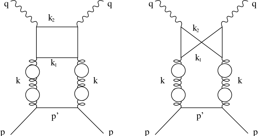
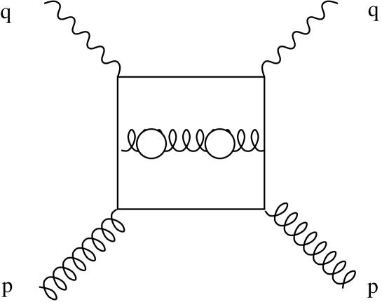
Explicit enumeration of the factors arising in both cases shows that contributions of the latter type are suppressed by a factor of as compared to the quark pure-singlet part. The large- structure of the quark pure-singlet coefficient can be written as
| (10) |
The curly brackets indicate the contribution in the expansion that comes from the fermion box. The gluonic coefficient is formally of the same order in . Taking into account that the lower vertex couples to the quark singlet or gluon structure function one obtains effectively an additional factor of in the former case. The quark singlet structure function is as compared with the gluon structure function 333We thank V.Braun for useful discussions about this point.. Recall, for example, that in the large- limit the fraction of longitudinal momentum carried by quarks and gluons is of the order and , respectively [36]. Following this argument one has to calculate only the quark singlet part as the dominating contribution in the large- limit.
Instead of calculating the corrections term by term to obtain the large-order behavior of the perturbative expansion, it is convenient to deal directly with the Borel transform of the whole series. In the special case we are considering here, there are two bubble chains which contribute, both having the same virtuality , see Fig. 1. By performing the substitution one easily obtains the Borel transform of the square of the running coupling
| (11) |
with , and being the Borel parameter. The Borel transform can be viewed as generating function for fixed order coefficients. Since our expansion starts at order the Borel transform vanishes at as it should be. Inserting Eq. (11) in the loop calculation this simple picture can be destroyed when collinear poles manifest itself as contributions which effectively simulate finite contributions to the Borel transform. Those poles are first to be subtracted to allow for the determination of fixed order results.
At this point it is convenient to discuss the equivalence between the renormalon approach and the finite gluon-mass method, where functions and are identified as coefficients of non-analytic terms in the small gluon-mass expansion of diagrams in Fig. 1. Note that in the present case both gluon chains depend on the same virtuality . Following [37], one can derive the Mellin representation of the square of the massive gluon propagator in the form:
| (12) |
which can be rewritten as
| (13) |
see Eq. (11). Inserting this equation into Eq. (16) below and inverting the resulting formula by means of the Laplace transformation, it is easy to see that the one-to-one correspondence between renormalon poles and non-analytic terms in the small gluon-mass expansion, discussed in [38], holds at the two-loop level as well. On the other hand, relation between the renormalon method and the effective coupling approach still requires further investigation [39].
To obtain the IR-renormalon poles from the diagrams in Fig. 1 we found it advantageous to follow the procedure for calculating DIS coefficient functions explained in [30, 40]. In this method the hadronic scattering tensor is calculated directly as the cross section of photon-parton scattering. Recall that in the partonic picture the hadronic structure functions can be written as
| (14) |
where and denote the bare parton density and the parton structure function corresponding to a parton . The parton structure function can be obtained order by order in the perturbation theory by calculating the radiative corrections to the parton subprocess
| (15) |
where a virtual photon of momentum hits a parton with momentum . In the general case, contains collinear divergences. They can be regularized e.g., by performing the calculation in dimensions. The dependence of on the regulator is indicated by the parameter . The infrared-divergent part has to be subtracted from the partonic cross-section and factored into the bare parton density to define a physical, measurable quantity. In the present calculation it is the Borel parameter which alters the power of the gluon propagator, and therefore regularizes divergent integrals. Because of that, it is sufficient to perform the calculation in dimensions. The collinear poles then show up as poles. Since we are only interested in the power corrections which manifest themselves as poles at , there is no need to calculate the subtractions explicitly. Note that the anomalous dimensions in the scheme do not exhibit renormalon singularities, and therefore the subtraction terms do not introduce additional renormalon poles [38, 41]. Hence, the IR-poles in the Borel image of structure functions arise only from the IR renormalon poles in the Borel image of partonic structure functions , calculated without subtractions.
Partonic structure functions can be obtained from the partonic tensor
| (16) |
where represents the -body phase space integration. The factor comes from averaging over quark spins in the unpolarized case. The tensor allows for an equivalent decomposition in terms of , , as the hadronic scattering tensor in Eq. (1). Choosing appropriate projections it holds:
| (17) |
The normalization is chosen such that in the simple parton model we get
| (18) |
3.1 Quark coefficient functions
To compute the pure-singlet contribution one needs to calculate the diagrams in Fig. 1. In the improved parton model this corresponds to the calculation of the two-to-three-body subprocess
| (19) |
which requires the three body phase space integrals
that appear in Eq. (16). It turns out to be convenient to evaluate the three particle phase space in the CMS system of the outgoing pair of the fermion box. Introducing variables as in [42] we find for the phase space integral
| (21) |
Here and are the polar and azimuthal angles in the CMS system of and respectively, while and are rescaled and channel invariants. The exact definition of theses variables can be found in the appendix of [42]. For our purpose the definition of
| (22) |
is important, where is the virtuality of the dressed gluon and is the argument of the partonic structure function . It follows that the Borel transforms of dimensionless projections of the partonic tensor Eq. (3) can be written in the form
| (23) |
which shows that the dependence on the Borel parameter factorises and is influenced only by the integration. To find the renormalon poles it is therefore not necessary to evaluate the whole expression exactly. Instead, we can expand in . The integration over transforms terms into simple poles and terms into double poles . Note that terms arise from the integration over the polar angle where partons and become collinear.
The expansion of in then leads to an expression of the form
| (24) |
The expansion coefficients and can be expressed as linear combinations
with the coefficients and being simple polynomials in . Inserting Eq. (24) back into Eq. (23) we observe that although the form of the phase space integral suggests that the Borel transform is simply proportional to , after performing the integration one actually obtains an expression of the form
It is interesting to note that the coefficient of the -pole in the sum over all diagrams vanishes, i.e. that the coefficient function of a DIS structure function does not contain any UV-renormalon poles. This is in line with previous observations that positions of UV-renormalon poles in NS-structure functions always depend on the Mellin moment [13], and that therefore UV-renormalon contributions are absent after the inverse Mellin transformation is performed.
Note the appearance of double poles in Eq. (3.1), which were not present in one-loop calculations of renormalon contributions to DIS structure functions in the non-singlet sector [13, 14, 15]. By considering renormalisation group improved version of OPE it can be shown that renormalon singularity of the Borel transform is in general expected to have the form [43]
| (26) |
Here corresponds to an eigenvalue of one-loop anomalous dimension matrix of higher twist operators of dimension which contribute to OPE of the hadronic tensor in Eq. (1). Calculation of anomalous dimensions considerably simplifies in the large- limit, resulting in eigenvalues which are either equal to zero or to a multiple of . The double pole found in Eq. (3.1) arises from operators with .
Terms in Eq. (3.1) singular at are directly related to singularities which occur in a calculation of in dimensions. The coefficient of the pole corresponds to the quadratic collinear divergence and is directly related to the pole in the usual dimensional regularization. In general, this coefficient can be written as a convolution of the leading order splitting functions
| (27) |
Thus, for the structure function one obtains
| (28) |
while for one finds
| (29) |
Note that for the longitudinal projections the fermion box is free of collinear divergences and therefore the contribution does not contain any pole.
The form of the constant term in the expansion can also be determined from general considerations. It is given by a combination of next to leading order splitting function and a convolution of leading order coefficient function and leading order splitting function corresponding to single poles. However, determination of the constant term in our approach requires the expansion to all orders given in Eq. (24).
Recall that for close to 1 one expects the ratio of twist-2 to twist-4 contributions to behave like , or approximately like [44]. The same trend at small would correspond to an expansion in terms of , see e.g. Ref. [45]. However, the exact calculation which takes into account Eq. (3.1) shows that in the small region the expansion parameter, see Eq. (3.1) below, turns out to be instead of . As a consequence, in the renormalon model the ratio of the twist-4 and twist-2 or the twist-6 and twist-4 contributions goes to a constant limit as . Note that in the renormalon model calculation of power corrections to parton fragmentation functions in anihilation into hadrons the expansion parameter turns out to be . Hence, the expansion breaks down in the region and has to be resummed [11]. No such resummation is required in the present case.
To obtain the coefficients in Eq. (2) one has to transform the Borel images back to the representation by using the inverse Borel transformation
| (30) |
An unambigious reconstruction of the perturbative expansion is prevented by the poles on the integration contour and therefore the summed series acquires an imaginary part which is directly related to the UV-divergent part of the higher twist operators we are looking for. Its magnitude can be estimated either directly or by taking the imaginary part (divided by ) of the inverse Borel transform in Eq. (30) [46]. This procedure leads, for the simple and quadratic poles of the right-hand side of Eq. (3.1), to
| (31) |
The ambiguity in the sign of the IR-renormalon contributions is due to the two possible contour deformations, namely above or below the pole at .
3.2 Gluon coefficient functions
As it has been mentioned above, the gluonic contribution is subleading in the large- limit. For finite , however, gluons certainly play an important role. To model their contribution we have adopted a procedure introduced in [11] in the analysis of power corrections in fragmentation processes in annihilation. The idea is to represent the pure-singlet unpolarized quark coefficient function as a convolution of the leading order quark-gluon unpolarized splitting function
| (32) |
with an effective gluonic unpolarized coefficient function . After taking Mellin moments of both sides of the equation
| (33) |
can be obtained by performing an inverse Mellin transformation of
| (34) |
The same procedure can be applied also to define the polarized gluon coefficient function , with the obvious modification that now the polarized pure-singlet quark coefficient function and the polarized quark-gluon splitting function
| (35) |
enter Eq. (34). The obtained formulae are presented in the appendix. In Fig. 3 and Fig. 4 we have compared the ratios of quark and gluonic twist-4 corrections to and to , respectively. It turns out that in both cases the shape of the gluon contribution which results from deconvolution procedure described above is quite similar to the shape of the original quark contribution. It is also easy to show that the ratio of quark and gluon contributions tends to a constant if . As the overall normalisation of each contribution is anyhow an adjustable fit parameter, we have modified the ratios in Fig. 3 and Fig. 4 by dividing in each case the quark contribution by a factor 2.


Note that this procedure results in the twist-4 contribution originated by gluons which depends linearly on the twist-2 gluon longitudinal momentum distribution. On the other hand, it has been known for a long time that an important class of twist-4 corrections to DIS originates from matrix elements of gluonic operators involving four gluon field strength tensors [19], thus being proportional to the square of the gluon momentum distribution. This is a good illustration of the fact that the renormalon model does not provide a description of all contributions to power suppressed corrections, and that some of the missed terms can be important for phenomenology.
4 Discussion
As it is known that the renormalon model cannot account for the absolute normalization of the twist-4 corrections, we follow the attitude proposed in [11, 18], and assume that model parameters, the overall normalization factors and mass scales, should be fitted to the data. Recall that in the flavour non-singlet case data at can be fitted using the normalization factor about 2 times larger than arising directly from the renormalon model. To get a feeling about the shape of pure flavour-singlet twist-4 corrections, in the following we discuss the renormalon model predictions for twist-4 corrections to , , and for a deuteron target, obtained at a fixed mass scale. For definiteness, we have used the NLO MRSA parameterization [47] and the NLO Gehrman-Stirling gluon-A set [48] at GeV2 as an input for twist-2 unpolarized and polarized parton distributions, respectively. We have checked that other sets of LO or NLO parton distributions produce similar results. While such an analysis cannot substitute for a data fit, it transparently reveals the gross features of the model.
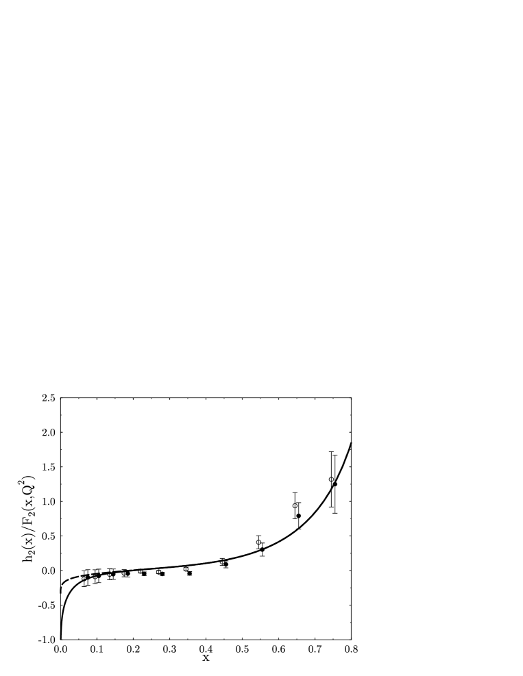
Fig. 5 shows the prediction for the ratio at GeV2 for a deuteron target as compared with the data from Ref. [3]. To obtain this plot we have fixed the sign in the right-hand side of Eq. (3.1), such that contributions arising from both simple and quadratic poles add coherently. At large the renormalon model prediction is dominated by contributions from NS-type graphs, common for singlet and non-singlet channels, see Eq. (9). It explains why it has been possible to fit deuteron and proton data in this domain by the renormalon model correction based only on the non-singlet coefficient function [14]. On the other hand, pure-singlet contributions dominate for smaller than 0.2. In the limit the ratio of twist-4 and twist-2 contributions tends to be a constant. We note that the contribution from the quadratic pole turns out to be larger than the contribution from the single one. If the pure-singlet quark contribution is replaced by a gluonic one, a very similar shape of twist-4 correction results, in accordance with the discussion in section 3.2. Figure 6 shows the same ratio with a logarithmic scale of the -axis.
Fig. 7 shows , the renormalon correction to plotted against the coefficient of the dependent term in the data fit of [49], for a deuteron target. The target mass correction taken from [50], makes up to 15%-20% of as compared to the phenomenological fit. The pure-singlet part becomes considerable only in the small region, where it produces a steep raise, clearly at variance with the parameterization of Ref. [49].


As expected, in the unpolarized case the pure-singlet contribution is negligible at large , but it dominates when becomes small. Although, strictly speaking, the absolute normalization is unknown, the renormalon model clearly suggests that while the non-singlet twist-4 contribution becomes smaller and smaller with decreasing, the magnitude of the pure-singlet contribution raises for below 0.2, and therefore twist-4 corrections should not be neglected in this region.
Recall that at large the UV dominance hypothesis predicts, in accordance with arguments based on an analysis of multiparton contribution of hadronic wave functions [44], that power corrections to are effectively suppressed by , and therefore they can be eliminated by a suitable cut-off. In the small- domain the situation is different. Our calculation predicts that the ratio of twist-4 to twist-2 terms in this region depends rather weakly on , such that the former cannot be minimized by a kinematical cut.
Here a natural question arises to which extent the renormalon model predictions can be trusted in the small domain. Although it is formulated in the field-theoretical framework, the model almost certainly misses some important QCD physics. We note e.g. that ladder corrections which are known to influence strongly the small behavior of twist-2 structure functions are absent here, as they are formally suppressed by . Hence, while we expect that general trends followed by twist-4 contributions are correctly reproduced, it is possible that details of small behavior of twist-4 corrections are not properly described in this approach.
Fig. 8 shows the renormalon model prediction for the twist-4 part of the polarized structure function . The resulting NS correction is negative at small , changes sign around , and reaches a maximum around . The pure-singlet contribution is significant only in the small region but, contrary to the unpolarized case, even there it does not dominate over the NS part. As in the case the ratio of twist-4 and twist-2 contributions to tends to be a constant for . In order to get a maximal magnitude of the pure-singlet correction, in Fig. 8 we have counted contributions from single and quadratic poles coherently.
5 Summary
The calculation presented in this paper extends previous renormalon model analyses of twist-4 corrections to DIS [12, 13, 14, 15] to the flavour singlet sector. We have presented a sample of predictions for the -dependence of twist-4 corrections to nucleon structure functions , , and in the whole domain. Our results suggest that in the small- region the twist expansion parameter is not , as it would follow from a -dependence of higher twist corrections, but is approximately equal to . In this case higher twists cannot be eliminated by a cut, and should be taken into account in the interpretation of the current data.
One possibility is to fit the data taking into account, in addition to twist-2 contribution, twist-4 corrections either in the form derived in the present paper with the non-singlet contribution taken from [14, 15], or as given in Ref. [21].
To obtain the renormalon model predictions for twist-4 corrections to nucleon structure functions in the flavour-singlet sector one should insert the pure-singlet coefficient functions, listed in the appendix below, into the right-hand side of Eq. (2), and add the non-singlet type contribution. For each contribution, the overall factor and its mass scale should be fitted independently. In particular, mass scales can be different for different channels. In principle one should also try a fit in which overall signs differ between contributions arising from single and quadratic poles. Because, as discussed in section 3.2, shapes of the resulting quark and gluon contributions are rather similar, such a fit could involve, besides standard parameterizations of the twist-2 structure functions at some low virtuality, only two additional elements: the quark non-singlet term, which can be taken from [14], and the gluonic term, as given below. Description of twist-4 corrections requires then the introduction of 3 new parameters: the normalization of the non-singlet quark contribution and the normalization and the mass scale which enters the gluonic contribution. In the currently most interesting case of a further simplification is possible: as the flavour non-singlet part is important only in the large- domain, it can be neglected in a fit to the small- data, which would reduce the number of additional fit parameters to 2.
Acknowledgements. This work has been supported by BMBF and DFG. We are indebted to V. Braun, L. Magnea, W. van Neerven and S. Forte for numerous interesting discussions. E.S. thanks DFG for support and the Department of Theoretical Physics of the University of Turin for the kind hospitality.
6 Appendix
In this section we quote explicitly our renormalon model results for the pure-singlet coefficient functions and , which control quark and gluon contributions to corrections to nucleon structure functions in the flavour singlet sector, see Eq. (2). For completeness, we quote also the coefficient functions and , arising from the second IR renormalon at , which can be used to model corrections.
To facilitate comparison with the data which treats contributions from single and quadratic poles separately, we have splitted each coefficient function into contributions arising from the single and quadratic poles, respectively.
6.1 Quark pure-singlet coefficient functions
Coefficient function for the quark pure-singlet renormalon contribution to : The contribution of the quadratic pole is proportional to .
Coefficient function for the quark pure-singlet renormalon contribution to : The first two lines contain the contribution from the single pole, the last line contains the contribution of the quadratic pole:
Coefficient function for the quark pure-singlet renormalon contribution to : The contribution of the quadratic pole is proportional to .
6.2 Gluon coefficients functions
In order to distinguish between contributions arising from single and quadratic poles we have split the coefficient functions explicitly into two parts, both proportional to . In addition, to keep the resulting expressions as compact as possible, we have introduced the notation
| (42) |
which appear often in the process of deconvoluting the unpolarized quark-gluon splitting function from the pure-singlet coefficient function.
Gluon coefficient functions for :
Gluon coefficient functions for :
Gluon coefficient functions for :
| (48) | |||||
References
-
[1]
D. H. Coward et al., Phys. Rev. Lett. 20, 292 (1968)
E. D. Bloom et al., Phys. Rev. Lett. 23, 930 (1969)
H. D. Breidenbach et al., Phys. Rev. Lett.. 23, 935 (1969) - [2] R. E. Taylor, Proc. Int. Sympo. on Lepton and photon interactions at high energies, Stanford, (1975)
- [3] M. Virchaux and A. Milsztajn, Phys. Lett. B274, 221 (1992)
-
[4]
H. D. Politzer, Phys. Rev. Lett. 30, 1346 (1973)
D. J. Gross and F. Wilczek, Phys. Rev. Lett. 30, 1323 (1973) -
[5]
R. L. Jaffe and M. Soldate, Phys. Rev. D26, 49 (1982)
R. K. Ellis, W. Furmanski, and R. Petronzio, Nucl. Phys. B207, 1 (1982)
E. V. Shuryak and A. I. Vainshtein, Nucl. Phys. B199, 451 (1982)
A. B. Bukhostov, G. V. Frolov, L. N. Lipatov, and E. A. Kuraev, Nucl. Phys. B258, 601 (1985)
I. I. Balitsky and V. M. Braun, Nucl. Phys. B311 (1988/89) 541 - [6] H. Georgi and H. D. Politzer, Phys. Rev. D14, 1829 (1976)
- [7] M. Göckeler, R. Horsley, E. M. Ilgenfritz, H. Perlt, P. Rakow, G. Schierholz, A. Schiller, Phys. Rev. D53, 2317 (1996)
- [8] G. Martinelli and C. T. Sachrajda, Nucl. Phys. B478, 660 (1996)
-
[9]
G. ’t Hooft, in ”The Whys of Subnuclear Physics,” Erice 1977,
ed. A.Zichichi (Plenum, New York 1977);
A.H. Mueller, The QCD perturbation series., in “QCD - Twenty Years Later”, edited by P.M. Zerwas and H.A. Kastrup, 162, (World Scientific 1992);
V. I. Zakharov, Nucl. Phys. B385 452 (1992);
A.H. Mueller, Phys. Lett. B308 355 (1993); -
[10]
M. Neubert, Phys.Rev. D51 5924 (1995)
M. Beneke, V.M. Braun, Nucl. Phys. B454 253 (1995)
R. Akhoury, V.I. Zakharov, Phys. Lett. B357 646 (1995)
C.N. Lovett-Turner, C.J. Maxwell, Nucl. Phys. B452 188 (1995)
N. V. Krasnikov, A. A. Pivovarov, Mod. Phys. Lett. A11 835 (1996)
P. Nason, M.H. Seymour, Nucl. Phys. B454 291 (1995)
P. Korchemsky, G. Sterman, Nucl. Phys. B437 415 (1995) - [11] M. Beneke, V. M. Braun, L. Magnea, Nucl. Phys. B497, 297 (1997)
- [12] Yu. L. Dokshitzer, G. Marchesini, B. R. Webber, Nucl. Phys. B469, 93 (1996)
- [13] E. Stein, M. Meyer-Hermann, A. Schäfer, L. Mankiewicz, Phys. Lett. B376, 177 (1996)
- [14] M. Dasgupta, B. R. Webber, Phys. Lett. B382, 273 (1996)
- [15] M. Meyer-Hermann, M. Maul, L. Mankiewicz, E. Stein, A. Schäfer Phys. Lett. B383, 463 (1996), Erratum-ibid. B393, 487 (1997)
- [16] B. R. Webber, Renormalon Phenomena in Jets and Hard Processes Talk given at 27th International Symposium on Multiparticle Dynamics (ISMD 97) hep-ph/9712236
- [17] V. I. Zakharov, Renormalons as a Bridge between Perturbative and Nonperturbative Physics Talk given at YKIS97, Kyoto, 97, hep-ph/9802416
- [18] M. Maul, E. Stein, A. Schäfer, L. Mankiewicz, Phys. Lett. B401, 100 (1997)
-
[19]
J. Bartels, Phys. Lett. B298, 204 (1993)
J. Bartels, Z. Phys. C60, 471 (1993) - [20] E. M. Levin, M. G. Ryskin, and A. G. Shuvaev, Nucl. Phys. B387, 589 (1992)
- [21] A. D. Martin, M. G. Ryskin, Higher Twists in Deep Inelastic Scattering, hep-ph/9802366
- [22] H1 Collaboration, Nucl. Phys. B497, 3 (1997)
- [23] ZEUS-Collaboration, J. Breitweg et al., Phys. Lett. B407, 432 (1997)
- [24] The New Muon Collaboration (NMC), M. Arneodo et al., Phys. Lett. B364, 107 (1995)
-
[25]
The New Muon Collaboration (NMC), M. Arneodo et al.,
Nucl. Phys. B483, 3, (1997)
The New Muon Collaboration (NMC), M. Arneodo et al., Nucl. Phys. B487, 3, (1997) - [26] M. Glück, E. Reya, A. Vogt, Z. Phys. C67, 433 (1995)
- [27] W. A. Bardeen, A. J. Buras, D. W. Duke, and T. Muta, Phys. Rev. D18, 3998 (1978)
- [28] C. Itzykson, J. -B. Zuber, Quantum Field Theory, McGraw Hill, New York,(1986)
- [29] W. R. Frazer, J. F. Gunion, Phys. Rev. Lett. B45, 1138 (1980)
- [30] E. B. Zijlstra and W. L. van Neerven, Nucl. Phys. B383, 525 (1992)
- [31] By S. A. Larin, P. Nogueira,T. van Ritbergen, J. A. M. Vermaseren, Nucl. Phys. B492, 338 (1997)
- [32] D. J. Broadhurst, Z. Phys. C58, 339 (1993)
- [33] M. Beneke Nucl. Phys. B405, 424 (1993)
- [34] M. Beneke and V. M. Braun, Phys. Lett. B348, 513 (1995)
- [35] F. Hautmann, Phys. Rev. Lett. 80, 3198 (1998)
- [36] M. E. Peskin and D. V. Schroeder, ’An Introduction to Quantum Field Theory’, Addison-Wesley (1995)
- [37] M. Beneke,V. M. Braun, V. I. Zakharov, Phys. Rev. Lett. 73, 3058 (1994)
- [38] P. Ball, M. Beneke, and V. M. Braun, Nucl. Phys. B452, 563 (1995)
- [39] L. Mankiewicz, E. Stein, in preparation.
- [40] G. Altarelli, R. K. Ellis, G. Martinelli, Nucl. Phys. B157, 461 (1979)
- [41] L. Mankiewicz, M. Maul, and E. Stein, Phys. Lett. B404, 345 (1997)
- [42] T. Matsuura, S. C. van der Marck, W. L. van Neerven, Nucl. Phys. B319, 570 (1989)
- [43] A. H. Mueller, Nucl. Phys. B250, 327 (1985)
- [44] E. L. Berger and S. J. Brodsky, Phys. Rev. Lett. 42, 940 (1979)
- [45] R. D. Ball, S. Forte, Phys.Lett. B405, 317 (1997)
- [46] V. M. Braun, QCD renormalons and higher twist effects. hep-ph/9505317 (1995)
- [47] A. D. Martin, R. G. Roberts and W. J. Stirling, Phys. Lett. B354, 155 (1995)
- [48] T. Gehrmann, W. J. Stirling, Phys. Rev. D53, 6100 (1996)
- [49] L. W. Whitlow, S. Rock, A. Bodek, S. Dasu, and E. M. Riordan, Phys. Lett. B250, 193 (1990)
- [50] J. Sanchez Guillen, J. L. Miramontes, M. Miramontes, G. Parente, and O. A. Sampayo, Nucl. Phys. B353, 337 (1991)