JLAB-THY-98-07

WM-98-102

QCD Evolution Equations: Numerical Algorithms from the Laguerre Expansion

Claudio Corianò^∗∗ and Cetin Savkli^∗∗†

^∗∗ Theory Group, Jefferson Lab, Newport News, VA 23606, USA

^† Dept. of Physics, College of William and Mary, Williamsburg, VA, 23187

A complete numerical implementation, in both singlet and non-singlet sectors, of a very elegant method to solve the QCD Evolution equations, due to Furmanski and Petronzio, is presented. The algorithm is directly implemented in x-space by a Laguerre expansion of the parton distributions. All the leading-twist distributions are evolved: longitudinally polarized, transversely polarized and unpolarized, to NLO accuracy. The expansion is optimal at finite x, up to reasonably small x-values ($x\approx 10^{-3}$), below which the convergence of the expansion slows down. The polarized evolution is smoother, due to the less singular structure of the polarized DGLAP kernels at small-x. In the region of fast convergence, which covers most of the usual perturbative applications, high numerical accuracy is achieved by expanding over a set of approximately 30 polynomials, with a very modest running time.

Program Summary

Title of the Programs: nsunpol, snunpol, nslong, snlong, trans

Computer:
Sun 19

Operating system: Unix

Programming language used: FORTRAN 77

Peripherals used: Laser Printer

Number of lines in distributed program: 4260

Keywords: Structure function, polarized parton distribution, $Q^{2}$ evolution, Laguerre expansions, numerical solution.

Nature of physical problem:
The programs provided here solve the DGLAP evolution equations, with next-to-leading order $\alpha_{s}$ effects taken to account, for unpolarized, longitudinally polarized and transversely polarized parton distributions.

Method of solution:
The method developed by Furmanski and Petronzio is used. The kernel $P(x)$ of the DGLAP integrodifferential equations and the evolution operators $E(t,x)$ are expanded in Laguerre polynomials.

Typical running time:
About 5 seconds for the transverse polarization case and 30 minutes for the longitudinal polarization and for the unpolarized.

LONG WRITE-UP

1 Introduction

The study of the spin structure of the proton is a fascinating aspect of the theory of the strong interactions. Parton distributions in the nucleon tell us about the structure of fundamental observables such as spin, parton densities and correlations among partons, in a light-cone framework. In a second quantized theory they emerge as matrix elements of nonlocal operators at light-like separations. At low energy they can be described by valence quark models and the impact of the QCD evolution (or Renormalization Group Evolution, RGE) on the shape of these distributions can be performed within the parton model.

It has become more and more common in the high energy literature to describe the evolution of parton distributions by starting from a low energy input.

There is widespread interest in the analysis of the effect of the QCD evolution especially for those leading twist distributions (such as the transverse spin distribution) which have not yet been measured. For instance, in ref. [5], the authors analize the impact of the evolution on transverse spin distributions derived at low $Q$ from the Isgur-Karl quark model [7], and these predictions can be used direclty -at very high energy- for other predictions, such as in the study of the transverse spin dependence of the Drell Yan process. A similar analysis can be done for the chiral quark model [6].

On the numerical side, various methods have been presented in the literature [10] which all try to solve the DGLAP equations by iterating the evolution over infinitesimal steps in the fractional momentum $x$. Another technique is based on the use of Mellin moments and on their inversion.In general, moments are equivalent to finite -rather than infinitesimal- discretizations of the integro-differential equations. In the case of the Mellin moments the inversion (to x-space) is the real difficult and time consuming part of the method.

A different, and very elegant implementation of methods based on finite discretizations of RGE’s for QCD was formulated long ago by Furmanski and Petronzio [2]. Their method uses the Laguerre expansion of the initial distributions and of the kernel of the evolution equations arrested to an arbitrary order $n$. The algorithm that they provide defines the structure of the moments recursively in terms of some initial conditions. In the non-singlet sector there have been attempts to apply the method both to leading and to next to leading order [18, 11], and to leading order in the singlet sector as well [18]. However, a complete implementation and numerical documentation of this algorithm is still missing. We also mention that our interest in this method has aroused from our search for the numerical implementations of more involved evolutions equations, such as those describing the dynamics of Compton scattering in the deeply virtual limit (DVCS) [9]. In this latter case, the RGE evolution is a continuous interpolation between 2 limits: the DGLAP (or Altarelli Parisi) evolution and the Efremov-Radyushkin-Brodsky-Lepage evolution (ERBL) [8]. We believe that a complete numerical understanding of these “non-diagonal” RGE’s and their robust numerical implementation requires finite step integrations. We hope to get back to this issue in the near future, and for the rest of this paper just focus on the usual DGLAP evolution. Here we have implemented the evolution of all the leading twist parton distributions, using the kernels calculated by various authors [2, 3, 13, 14]. A complete list of these kernels can be found in the Appendix.

2 The Laguerre expansion

The Laguerre method for the numerical solution of the evolution equations is due to Furmanski and Petronzio. In this section we briefly outline the method, which is fast converging at intermediate values of x and any $Q^{2}$ value. At very small-x (approximately $10^{-3}$), the Laguerre expansion suffers from numerical instabilities, due to the growth of the moments. We start by defining our notation and other conventions.

The two-loop running of the coupling constant is defined by

$${\alpha(Q_{0}^{2})\over 2\pi}={2\over\beta_{0}}{1\over\ln(Q^{2}/\Lambda^{2})}\left(1-{\beta_{1}\over\beta_{0}}{\ln\ln(Q^{2}/\Lambda^{2})\over\ln(Q^{2}/\Lambda^{2})}+O({1\over\ln^{2}(Q^{2}/\Lambda^{2})})\right).$$ (1)

where

$$\beta_{0}={11\over 3}C_{G}-{4\over 3}T_{R}n_{f}$$

$$\beta_{1}={34\over 3}C_{G}^{2}-{10\over 3}C_{G}n_{f}-2C_{F}n_{f}$$ (2)

where

$$C_{G}=N,\,\,\,\,\,\,\,C_{F}={N^{2}-1\over 2N},\,\,\,\,\,\,\,\,T_{R}={1\over 2}$$ (3)

and N is the number of colours.

The solution for the running coupling is given by

$$\alpha(t) = {\alpha(0)\over 2\pi}e^{-\beta_{0}/2t}$$ (4)

with $\alpha(Q_{0}^{2})\equiv\alpha(0)$, and $Q_{0}$ denoting the initial scale at which the evolution starts. The evolution equations are of the form

$$Q^{2}{d\over dQ^{2}}{q_{i}}^{(-)}(x,Q^{2}) = {\alpha(Q^{2})\over 2\pi}P_{(-)}(x,\alpha(Q^{2}))\otimes q_{i}^{(-)}(x,Q^{2})$$

$$Q^{2}{d\over dQ^{2}}\chi_{i}(x,Q^{2}) = {\alpha(Q^{2})\over 2\pi}P_{(-)}(x,\alpha(Q^{2}))\otimes\chi_{i}(x,Q^{2})$$

with

$$\chi_{i}(x,Q^{2})={q_{i}}^{(+)}(x,Q^{2})-{1\over n_{F}}q^{(+)}(x,Q^{2})$$ (6)

for the non-singlet distributions and

$$Q^{2}{d\over dQ^{2}}\left(\begin{array}[]{c}q^{(+)}(x,Q^{2})\\ G(x,Q^{2})\end{array}\right)=\left(\begin{array}[]{cc}P_{qq}(x,Q^{2})&P_{qg}(x,Q^{2})\\ P_{gq}(x,Q^{2})&P_{gg}(x,Q^{2})\end{array}\right)\otimes\left(\begin{array}[]{c}q^{(+)}(x,Q^{2})\\ G(x,Q^{2})\end{array}\right)$$ (13)

for the singlet sector.

We have defined, as usual

$$q_{i}^{(-)}=q_{i}-\bar{q}_{i},\,\,\,\,\,q^{(+)}_{i}=q_{i}+\bar{q}_{i},\,\,\,\,\,\,q^{(+)}\equiv\Sigma=\sum_{i=1}^{n_{f}}q^{(+)}_{i}.$$ (15)

We introduce the evolution variable

$$t=-{2\over\beta_{0}}\ln{\alpha(Q^{2})\over\alpha(Q_{0}^{2})}$$ (16)

which replaces $Q^{2}$. The evolution equations are then rewritten in the form

$${d\over dt}q_{i}^{(-)}(t,x) = \left(P^{(0)}(x)+{\alpha(t)\over 2\pi}R_{(-)}(x)+...\right)\otimes q_{i}^{(-)}(t,x)$$ (17)

$$Q^{2}{d\over dt}\chi_{i}(x,Q^{2}) = \left(P^{(0)}(x)+{\alpha(t)\over 2\pi}R_{(+)}(x)\right)\otimes\chi_{i}(x,Q^{2}),$$ (18)

$${d\over dt}\left(\begin{array}[]{c}q^{(+)}(t,x)\\ G(x,t)\end{array}\right) = \left(P^{(0)}(x)+{\alpha(t)\over 2\pi}R(x)+...\right)\otimes\left(\begin{array}[]{c}q^{(+)}(x,t)\\ G(x,t)\end{array}\right).$$ (23)

In the new variable $t$, the kernels of the evolution take the form

$$R_{(\pm)}(x) = P^{(1)}_{(\pm)}(x)-{\beta_{1}\over 2\beta_{0}}P^{(0)}_{V}(x)$$

$$R(x) = P^{(1)}(x)-{\beta_{1}\over 2\beta_{0}}P^{(0)}(x).$$ (24)

Equations (17) and (18) are solved independently for the variables $q_{i}^{(-)}$ and $\chi_{i}$ respectively. Finally, the solution $q^{(+)}$ of eq. (23) (or the singlet equation) is substitued into $\chi_{i}$ in order to obtain $q_{i}^{(+)}$. The equations can be written down in terms of two singlet evolution operators $E_{\pm}(t,x)$ and initial conditions $\tilde{q}_{\pm}(x,t=0)\equiv\tilde{q}_{\pm}(x)$ as

$${d\over dt}E_{\pm}=P_{\pm}\otimes E_{\pm},$$ (25)

whose solutions are given by

$$q_{i}^{(-)}(t,x)=E_{(-)}\otimes\tilde{q}_{i}^{(-)}$$

$$\chi_{i}(t,x)=E_{(+)}\otimes\tilde{\chi}_{i}(x).$$ (26)

The singlet evolution for the matrix operator $E(t,x)$

$$\left(\begin{array}[]{cc}E_{FF}&E_{FG}\\ E_{GF}&E_{GG}\end{array}\right)$$ (29)

$${dE\over dt}=P\otimes E$$ (30)

is solved similarly as

$$\left(\begin{array}[]{c}q^{(+)}(t,x)\\ G(t,x)\end{array}\right)=E(t,x)\otimes\left(\begin{array}[]{c}\tilde{q}^{(+)}(x)\\ \tilde{G}(x)\end{array}\right).$$ (35)

The method of Furmanski and Petronzio requires an expansion of the splitting functions and of the parton distributions in the basis of the Laguerre polynomials

$$L_{n}(y)=\sum_{k=0}^{n}\left(\begin{array}[]{c}n\\ k\end{array}\right)(-1)^{k}{y^{k}\over k!}$$ (37)

which satisfies the property of closure under a convolution

$$L_{n}(y)\otimes L_{m}(y)=L_{n+m}(y)-L_{n+m+1}(y).$$ (38)

In order to improve the small-x behaviour of the algorithm, from now on, the evolution is applied to the modified kernel $xP(x)$, which, for simplicity, is still denoted as in all the equations above, i.e. by $P(x)$. At a second step, the $0<x<1$ interval is mapped into an infinite interval $0<y<\infty$ by a change of variable $x=e^{-y}$ and all the integrations are performed in this last interval. We start from the non-singlet case by defining the Laguerre expansion of the kernels and the corresponding (Laguerre) moments to lowest order

$$P_{V}^{(0)}(y) = \sum_{n=0}^{\infty}P_{n}^{(0)}L_{n}(y),$$

$$P_{n}^{(0)} = \int_{0}^{\infty}dye^{-y}L_{n}(y)\,\,P^{(0)}(y)$$ (39)

and to NLO

$$R(y)=\sum_{n=0}^{\infty}R_{n}L_{n}(y).$$ (40)

One defines also the difference of moments

$$p_{i}^{(0)} = P_{i}^{(0)}-P_{i-1}^{(0)}\,\,\,\,\,\,\,(P_{-1}^{(0)}=0)$$

$$r_{i} = R_{i}-R_{i-1}\,\,\,\,\,\,R_{-1}=0.$$ (41)

A similar expansion is set up for the evolution operators $E(t,y)$

$$E^{(0)}(t,y) = \sum_{n=0}^{\infty}E_{n}^{(0)}(t)L_{n}(y)$$

$$E(t,y) = \sum_{n=0}^{\infty}E_{n}(t)L_{n}(y),$$ (42)

where all the information on the $t$ evolution is contained in the moments $E_{n}(t)$. The solution to NLO is expressed as [4]

$$E_{n}(t)=E_{n}^{(0)}(t)-{2\over\beta_{0}}{\alpha(t)-\alpha(0)\over 2\pi}E_{n}^{(1)}(t),$$ (43)

where

$$E_{n}^{(0)}(t)=e^{P_{0}^{(0}t}\sum_{k=0}^{n}{A_{n}^{(k)}t^{k}\over k!}$$ (44)

$$E_{n}^{(1)}(t)=\sum_{i}^{n}r_{n-i}E_{i}^{(0)}(t),$$ (45)

and the coefficients $A_{n}^{(k)}$ are determined recursively from the moments of the lowest order kernel $P^{(0)}$

$$A_{n}^{(0)} = 1$$

$$A_{n}^{(k+1)} = \sum_{i=k}^{n-1}p_{n-i}^{(0)}A_{i}^{(k)}\hskip 28.45274pt(k=0,1,2,...,n-1).$$ (47)

In the singlet case one proceeds in a similar way. The solution is expressed in terms of a 2-by-2 matrix operator

$$E^{(0)}(t,y)=\sum_{n=0}^{\infty}E_{n}^{(0)}(t)L_{n}(y).$$ (48)

The solution (at leading order) is written down in terms of 2 projection matrices and one eigenvalue ($\lambda$) of the $P^{(0)}$ (matrix) kernel

$$e_{1}={1\over\lambda}P^{(0)},\hskip 56.9055pte_{2}={1\over\lambda}\left(-P^{(0)}+\lambda\bf{1}\right),$$ (49)

where

$$\lambda = -({4\over 3}C_{F}+{2\over 3}n_{f}T_{R}),$$ (51)

in the form

$$E^{(0)}_{n}(t) = \sum_{k=0}^{n}{t^{k}\over k!}\left(A_{n}^{(k)}+B_{n}^{(k)}e^{\lambda t}\right).$$ (52)

The recursion relations which allow to build $A_{n}^{(k)}$ and $B_{n}^{(k)}$ are solved in two steps as follows. One solves first for two sets of matrices $a_{n}^{(k)}$ and $b_{n}^{(k)}$ by the relations

$$a_{n}^{(0)} = 0$$

$$a_{n}^{(k+1)} = \lambda e_{1}a_{n}^{(k)}+\sum_{i=k}^{n-1}p_{n-i}^{(0)}a_{i}^{(k)}$$

$$b_{n}^{(0)} = 0$$

$$b_{n}^{(k+1)} = -\lambda e_{2}b_{n}^{(k)}+\sum_{i=1}^{n-1}p_{n-i}^{(0)}b_{i}^{(k)},$$ (53)

which are used to construct the matrices $A_{n}^{(0)}$ and $B_{n}^{(0)}$

$$A_{n}^{(0)} = e_{2}-{1\over\lambda^{n}}\left(e_{1}a_{n}^{(n)}-(-1)^{n}e_{2}b_{n}^{(n)}\right)$$

$$B_{n}^{(0)} = e_{1}+{1\over\lambda^{n}}\left(e_{1}a_{n}^{(n)}-(-1)^{n}e_{2}b_{n}^{(n)}\right).$$ (54)

These matrices are then input in the recursion relations

$$A_{0}^{(0)} = e_{2}\hskip 28.45274ptB_{0}^{(0)}=e_{1}$$

$$A_{n}^{(k+1)} = \lambda e_{1}A_{n}^{(k)}+\sum_{i=k}^{n-1}p_{n-i}^{(0)}A_{i}^{k}$$

$$B_{n}^{k+1} = -\lambda e_{2}B_{n}^{(k)}+\sum_{i=k}^{n-1}p_{n-i}^{(0)}B_{i}^{(k)}$$ (56)

witn $n>0$ and $k=0,1,...,n-1$, which generates the coefficients of the matrix-valued operator $E^{(0)}$ (i.e. the leading order solution). The NLO part of the evolution is obtained from

$$E^{(1)}(t,y) = \sum_{n=0}^{\infty}E_{n}^{(1)}(t)L_{n}(y),$$ (57)

with

$$E_{n}^{(1)}(t) = \tilde{E}_{n}^{(1)}(t)-2\tilde{E}_{n-1}^{(1)}(t)+\tilde{E}_{n-2}^{(1)}(t)$$ (58)

where

$$\tilde{E}_{n}^{(1)}(t)=\int_{o}^{t}d\tau e^{-\beta_{0}\tau/2}\sum_{ijk}E^{(0)}(t-\tau)R_{j}E_{k}^{(0)}(\tau)\delta(n-i-j-k).$$ (59)

The expressions of $E^{(0)}$ and $E^{(1)}$ are inserted into eq. (43) thereby providing a complete NLO solution of the singlet sector.

3 The polarized and the unpolarized evolution

The implementation of the polarized and of the unpolarized evolution is performed in the $\overline{MS}$ scheme, which is by now standard in most of the high energy physics applications. In the unpolarized case, we introduce valence quark distributions $q_{V}(x,Q_{0}^{2})$ and gluon distributions $G(x,Q_{0}^{2})$ at the input scale $Q_{0}$, taken from the CTEQ parametrization [25]

$$q(x) = A_{0}x^{A_{1}}(1-x)^{A_{2}}(1+A_{3}x^{A_{4}}).$$ (60)

Specifically

$$xu_{V}(x) = 1.344x^{0.501}(1-x)^{3.689}[1+6.042x^{0.873}]$$

$$xd_{V}(x) = 0.640x^{0.501}(1-x)^{4.247}[1+2.690x^{0.333}]$$

$$xG(x) = 1.123x^{-0.206}(1-x)^{4.673}[1+4.269x^{1.508}]$$ (61)

and an asymmetric sea contribution

$$x\overline{q}(x) = {1\over 2}[0.255x^{-0.143}(1-x)^{8.041}(1+6.112x)\mp 0.071x^{0.501}(1-x)^{8.041}],$$ (62)

where the $(-)$ holds for the $\bar{u}$ and the $(+)$ for the $\bar{d}$ flavors. The set accounts for a $\bar{u},\bar{d}$ flavour asymmetry, and the sea quark contribution is parameterized by

$$x\bar{s}(x) = [0.064x^{-0.143}(1-x)^{8.041}(1+6.112x)].$$ (63)

In the polarized case we have chosen the first set of ref. [20] which is of the functional form $ABx^{C}(1-x)^{D}(1+Ex+F\sqrt{x})$

$$x\Delta u_{V} = 0.918*1.365*x^{0.512}(1-x)^{3.96}(1+11.65x-4.6\sqrt{x})$$

$$x\Delta d_{V} = -0.339*3.849x^{0.78}(1-x)^{4.96}(1+7.81x-3.48\sqrt{x})$$

$$x\Delta G = 1.71*3.099x^{0.724}(1-x)^{5.71}(1+0.0x+0.0\sqrt{x}).$$ (64)

For the (flavour symmetric) sea contribution we have set $\Delta\bar{u}=\Delta\bar{d}=\Delta\bar{s}$ with

$$\Delta\bar{s}=-0.06*18.521x^{0.724}(1-x)^{14.4}(1+4.63x-4.96\sqrt{x}).$$ (65)

Notice that the evolution in the $\overline{MS}$ requires some care, depending upon the way the subtraction of the collinear singularities in the coefficient functions (hard scatterings) is performed. The (non singlet) hard scatterings, in fact, do not conserve helicities in the annihilation channels. In a “traditional” $\overline{MS}$ scheme, one has to keep both these helicity violating terms of the coefficient functions and has add to the polarized non-singlet kernels of the Appendix some additional terms proportional to $(1-x)$ to NLO [15, 17, 13] As a result of this, both the singlet and the non-singlet evolution are affected to NLO. However, one can factorize out of the coefficient functions these spuriuos (helicity-violating) terms and absorb them into the renormalization of the parton distributions. As a result of this procedure, the NLO kernels of the evolution turn out to be exactly those defined in the Appendix and the hard-scatterings are helicity preserving.

4 The evolution of the transverse spin distribution

The first identification of the transverse spin distribution is due to Ralston and Soper [23] in their study of the factorization formula for the Drell Yan cross section. The parton interpretation of this distribution has been discussed in various papers [16, 24], in which its behaviour as a leading twist distribution has been pointed out.

It appears in the double transverse spin asymmetry $A_{TT}$ for the Drell Yan process [23, 24]

$$A_{TT}={\sin^{2}\theta\cos 2\phi\over 1+\cos^{2}\theta}{\sum_{i}e_{i}^{2}\Delta_{T}q_{i}(x_{1})\Delta_{T}\bar{q}_{i}(x_{2})\over\sum_{i}e_{i}^{2}q_{i}(x_{1})\bar{q}_{i}(x_{2})}.$$ (66)

In eq. (66) the angles $\theta$ and $\phi$ are the polar and the azimuthal angles of the momentum of one of the two leptons, measured with respect to the beam ($\theta$) and to the photon polarization directions ($\phi$). The asymmetry disappears if the momenta of the two leptons are both integrated over. In the parton model, $\Delta_{T}(q)$ is interpreted as the probability of finding a quark with spin polarized along the transverse spin of a transversely polarized proton minus the probability to find it polarized oppositely. This distribution does not couple to gluons and is therefore, purely non-singlet. The LO anomalous dimensions of this distribution have been calculated in [16], while the NLO corrections have been derived by various authors [17], using both the Operator Product Expansion and the method of ref. [12], extended to the polarized case.

Since the gluons don’t couple in the evolution, the equation is simply written as

$${\partial\over\partial\ln Q^{2}}\Delta_{T}q_{\pm}(x,Q^{2})={\alpha_{s}(Q^{2})\over 2\pi}\Delta_{T}P_{q^{\pm}}(x)\otimes\Delta_{T}q_{\pm}(x,Q^{2}).$$ (67)

As in the previous sections, we have set $\Delta_{T}q_{\pm}=\Delta_{T}q\pm\Delta_{T}\bar{q}$.

5 Description of the program

The first step in the calculation is the computation of Laguerre moments -or expansion coefficients- of the kernel which are given by an explicit recursion relation.

The solutions of the integral equations are obtained by first discretizing the integrals in the form

$$\int dq\,f(q)\longrightarrow\sum_{i=1}^{n}w_{i}\,f(q_{i}),$$ (68)

where $w_{i}$ are integration weights for the grid-points $q_{i}$. Various sets of Gauss-Legendre grid-points are provided (by the GAUSS and the LEGENDRE subroutines) in the interval $(-1,1)$ . In order to map the grid points and the weights from the interval $(-1,1)$ to the interval $(0,\infty)$, one can use various mappings. The possible types of mapping provided in the code are
(i) MAPNO=1:

$$y(x)=R_{min}+\frac{(1+x)}{1-x+2/(R_{max}-R_{min})},$$ (69)

(ii) MAPNO=2:

$$y(x)=R_{min}+(R_{max}-R_{min})*(x+1)/2,$$ (70)

(iii) MAPNO=3 (Ref. [21, 22]):

$$y(x)=R_{min}+\frac{R_{d}{\rm tan}(\frac{\pi}{4}(1+x))}{1+\frac{R_{d}}{R_{max}-R_{min}}{\rm tan}(\frac{\pi}{4}(1+x))},$$ (71)

where

$$R_{d}=\frac{R_{med}-R_{min}}{R_{max}-R_{med}}(R_{max}-R_{min}).$$ (72)

Because of its flexibility, we use the tangent mapping. According to the tangent mapping,

$$y(-1)=R_{min},\,\,y(0)=R_{med},\,\,y(1)=R_{max}.$$ (73)

Therefore, one can safely control the range $(R_{min},R_{max})$ and the distribution $(R_{med})$ of the grid points. With this discretization procedure, continuous integral equations are transformed into nonsingular matrix equations.

6 Description of input parameters and input distribution

6.1 Input parameters

NF	Number of quark flavors
NGRID	Number of grid points
PLQCD	$\Lambda_{qcd}$
Q2I	Initial $Q^{2}$
Q2F	Final $Q^{2}$
RMIN	Smallest grid point
RMED	Median of grid poiunts
RMAX	The maximum grid point
LN	The highest degree of Laguerre polynomial included

IFLAV	1	u quark
	2	d quark
	2	s quark
MAPNO	1	type-1 mapping
	2	linear mapping
	3	tangent mapping
IALPH	0	leading order (LO) in $\alpha_{s}$
	1	next-to-leading order (NLO) in $\alpha_{s}$

6.2 Arrays

P(I)	Grid points $y=P(I)$, where $RMIN<P(I)<RMAX$
WP(I)	Weights
PT(I)	Grid points $t=PT(I)$, where $0<t<T=-2/\beta_{0}\ln(\alpha_{s}(q^{2})/\alpha_{s}(q^{2}_{0}))$
WT(I)	Weights
PN(LN,IE,JE)	elements of the LN’th Laguerre moment of LO kernel $[P]_{2\times 2}$
RN(LN,IE,JE)	elements of the LN’th Laguerre moment of NLO kernel $[R]_{2\times 2}$
SPN(I,IE,JE)	PN(I,IE,JE)- PN(I-1,IE,JE)
E1(J,K)	PN(0,J,K)/$\lambda$
E2(J,K)	-PN(0,J,K)/$\lambda$
SA(K,N,IE,JE)	$[a^{k}_{n}]_{2\times 2}$
SB(K,N,IE,JE)	$[b^{k}_{n}]_{2\times 2}$
A(K,N,IE,JE)	$[A^{k}_{n}]_{2\times 2}$
B(K,N,IE,JE)	$[B^{k}_{n}]_{2\times 2}$
ENT(I,IE,JE)	$[E_{n}(t)]_{2\times 2}$
PHI0(Y,IE)	Initial distributions $x\Delta\Sigma_{0}$, $x\Delta G_{0}$ respectively for $IE=1,2$
PHI0N(N,IE)	Laguerre moments of initial distribution.
PHIT(I,IE)	Evolved distributions $x\Delta\Sigma$, $x\Delta G$ respectively for $IE=1,2$

The codes provided are stored in three directories named after the polarization types; namely transverse, longitudinal and unpolarized. In each directory there are exacutable files that can be used to compile the fortran codes (executable file “comp”) and run them (executable file “run”). The transverse polarization case is the simplest. For transverse polarization one has only the nonsinglet equation. In the longitudinally polarized and unpolarized cases both singlet and nonsinglet equations are solved. The solutions of the singlet and nonsinglet equations are provided by separate codes. For the longitudinally polarized case the nonsinglet equation is solved by “nslong.f”, while the singlet equation is solved by “snlong.f”. Both codes use the same input file, which is called “INPUT”. Nonsinglet and singlet equations work in coordination with each other. Upon execution of the “run” command, first the nonsinglet equation is solved, and the output is written into data files. Next the nonsinglet equation is solved. The data produced by the solution of the singlet equation is read by the code which solves the nonsinglet equation. The user is expected to prepare the “INPUT” file, compile the codes by using command “comp” and then run them using the command “run”. The procedure for the unpolarized case is the same, with the only difference being the names of the files which are “nsunpol.f” and “snunpol.f”. Next, we give the detailed descriptions of the programs “sn*.f”

7 SNLONG and SNUNPOL

Since the only difference between these programs are the kernels and the initial conditions, the explanations provided below equally apply to both.

7.1 Main Program

The main program starts by calling the INPUT subroutine. This subroutine reads 12 input parameters described in Table 6.1. Next, the grid points and the weights are calculated by calling the subroutine GAUS, and they are mapped into the desired interval. The mapping is done by the MAP subroutine.

Then, in order to calculate the Laguerre moments of the kernel and input distributions, the subroutine XPL is called. The factors $A^{k}_{n}$, $B^{k}_{n}$ which are used in the construction of the leading order evolution operator $E^{0}_{n}$ are calculated in a subroutine called XBKN. In the next step, the XEN subroutine is called to calculate the evolution operator $E_{n}$. Finally, the evolution of the initial distribution is performed in the VQD subroutine. The results for the evolved distributions $\Delta\Sigma(x)$, and $\Delta G(x)$ are written, respectively, into the files “dltsig.dat”, and “dltglu.dat”. Later, the result for the $\Sigma$ distribution is read by the program that solves the nonsinglet equation.

7.2 Subroutine INPUT

In this subroutine 12 input parameters are read. In addition to reading these parameters, various constants to be used throughout the program are also defined in the INPUT subroutine. These constants are ${\rm PLQCD}=\lambda_{QCD}$, ${\rm PI}=\pi$, ${\rm Z3}=\zeta_{3}$, CF, CG, CA, TR, ${\rm BT0}=\beta_{0}$, ${\rm BT1}=\beta_{1}$, $T=-2/\beta_{0}\ln(\alpha_{s}(q^{2})/\alpha_{s}(q^{2}_{0}))$, and ${\rm XLMBD}=\lambda$.

7.3 Subroutine XPL

In this subroutine we calculate the Laguerre moments of the initial distributions PHI0(Y,IE) and kernels $P_{0}$ and $R=P_{1}-\beta_{1}/(2\beta_{0})P_{0}$. In PHI0(Y,IE),

$$Y=\ln(1/X)\equiv P(J),$$ (1)

and the IE index is used to label the initial distributions for $x\Delta\Sigma(x)$(IE=1), and $x\Delta G(x)$(IE=2). We use variable $Y=[0,\inf)$ rather than $X=[0,1]$ in calculating the Laguerre moments. The results for the Laguerre moments of the initial distributions are stored in PHI0N(I,IE) where $IE=1,2$ corresponds to the Laguerre moments of $x\Delta\Sigma,x\Delta G$ respectively, and $I$ refers to the order of Laguerre moments. In order to calculate the Laguerre moments of the kernel, we express it in the following form

$$P=P_{r}+\frac{P_{s}}{(1-x)_{+}}+P_{\delta}\delta(1-x).$$ (2)

The singular part $P_{s}$ is regulated according to the “+” regularization prescription, while the regular part $P_{r}$ is directly integrated. The delta function part requires no numerical integration. Therefore, the contribution of this piece is trivially added after performing the numerical integrals for $P_{r}$ and $P_{s}$. The kernels are stored in the arrays P0R(Y,IE,JE), P0S(Y,IE,JE), P1R(Y,IE,JE), P1S(Y,IE,JE), where “R” and “S” stand for the “regular” and “singular” parts of the kernels, and $IE=1,2$, $JE=1,2$ are matrix indices. According to our convention, the distributions are introduced by define $2\times 1$ vector array as $(x\Delta\Sigma,x\Delta G)$. In this subroutine we also define the arrays SPN(I,IE,JE), E1(J,K), and E2(J,K).

7.4 Subroutine XBKN

In this subroutine we construct the arrays SA(K,N,IE,JE), SB(K,N,IE,JE), A(K,N,IE,JE), B(K,N,IE,JE) using nested loops.

7.5 Subroutine XEN

This is the subroutine where the Laguerre moments of the evolution operator, ENT(N,IE,JE), are constructed. In this subroutine the functions E0N(N,T,IE,JE) and E1N(N,T,IE,JE) are called. These functions represent the 0th and 1st order contributions to the Laguerre moments.

7.6 Function E0N(N,T,IE,JE)

Calculates E0N(N,T,IE,JE) using the previously calculated A(K,N,IE,JE), and B(K,N,IE,JE) arrays. Notice that we have defined E0N(N,T,IE,JE) as a function rather than a subroutine. The reason for this is the following: E0N(N,XT,IE,JE) appears inside an integral in the calculation of E1N(N,T,IE,JE), where XT($0<XT<T$) is the integration variable. Therefore, on needs to know E0N for all possible values of XT.

7.7 Function E1N(N,T,IE,JE)

Calculates E1N. The set of grid points for the XT integral is PT(I), and the weights are WT(I). Grid points, which was determined in the mained program using Gauss-Legendre subroutines, are chosen such that $0<PT(I)<T$.

7.8 Subroutine VQD

Evaluates the final result PHIT(I,IE) for evolved distributions. Here, “I” represents the x (Bjorken) value, where $x=e^{(}-P(I))$, and IE as usual refers to two different parton distributions, that is $PHIT(I,1)=xG(x)$, and $PHIT(I,2)=x\Sigma(x)$ (IE=2).

7.9 Functions XLAG, FCTRL, S2, S1, ST

XLAG(N,Y) computes the Laguerre polynomial of order N at Y. FCTRL(N) computes N!. The result is given in double precision. S2(X) and S1(x) are respectively the functions $S_{1}(x)$, and $S_{2}(x)$. ST(x) represents $\tilde{S}(x)$.

7.10 Other functions

We also define various simple functions which are used throughout the program. $ALPHAS(Q^{2})$ is $\alpha_{s}(Q^{2})$. GS(X,A,B,C,D,E,F) is the Gehrmann-Stirling ansatz “A” [20] for the polarized parton distributions. In addition, for convenience in typing in the kernel for longitudinal parton distributions, we define PF(X), PGS(X), PGR(X), PNFS(X), PNFR(X), PA(X), FQQ(X), F1QG(X), F2QG(X), F1GQ(X), F2GQ(X), F3GQ(X), F1GGS(X), F1GGR(X), F2GG(X), F3GGS(X), F3GGR(X).

7.11 subroutines GAUSS, LEGENDRE and MAP

The LEGEND(X,L,PSUBL) subroutine computes Legendre polynomials of argument x from 0 to order L. The GAUS(Y,WY,N) subroutine determines N gaussian points(in the vector Y) and N weights(in the vector WY). For this routine N must be even and not greater than 100. Since the points and weights are symmetric about zero, only half are stored. The original version of this subroutine was written by S. Cotanch [19], at the Univ. of Pittsburgh in the years 1974-75. The MAP(Y,WY,N,MTYPE,RMIN,RMAX,RMED) subroutine maps the initial set of N grid points Y(I) and weights WY(I) to the desired interval (RMIN,RMAX). As explained in detail earlier, the mapping type MTYPE=3 allows one to control the median(RMED) of the distribution. For the Y variable that we use in calculating the Laguerre moments, we have used RMIN=0.0D0, RMAX=1.0D2, and RMED=5.0d0 Since the Laguerre moment integrals are damped by exponential factors $e^{-Y}$, RMAX=1.0D2 was a large enough cutoff for the integral.

8 NSLONG and NSUNPOL

The structure of the codes NSLONG and NSUNPOL are the same as that of SNLONG and SNUNPOL. All subroutine names and their functions are identicle. The only major difference comes from the fact that in the nonsinglet case one no longer has a matrix equation. Rather, there are two uncoupled equations. The nonsinglet codes read the $x\Sigma(x)$ results which are produced by the singlet codes.

9 Running the code

In order to get reliable results for $0.001<x<1$ we have used approximately 30 Laguerre polynomials. The number of grid points used was $N=60$. The nonsinglet codes run in about 1 minute. The singlet and nonsinglet codes together run in about 20 minutes. At very small x $(x<0.001)$ the Laguerre polynomials diverge, and therefore they are not a convenient basis to use in the very small x region. However, for $0.001<x<1$, the results are stable for a reasonable number of Laguerre polynomials.

10 Conclusions

We have shown that the Laguerre expansion is a significant tool in the analysis of the QCD evolution equations from the numerical side. These advantages include both short running times in the actual implementation of the evolution and the possibility to have well defined recursion relations. The Laguerre algorithm is a very powerful way to address efficiently these problems.

We remark that polynomial expansions are going to be of wide use in the analysis of more general parton distributions -such as the non-forward or the double distributions- which have been introduced in the recent literature on Compton processes. Here we have just began our tour on the analysis of QCD renormalization group equations and their solutions by finite step integrations. We hope to return to the study of the extension of these methods to the non-diagonal partonic evolution in the near future.

Acknowledgements

We are grateful to L.E. Gordon, Gordon Ramsey for discussions.

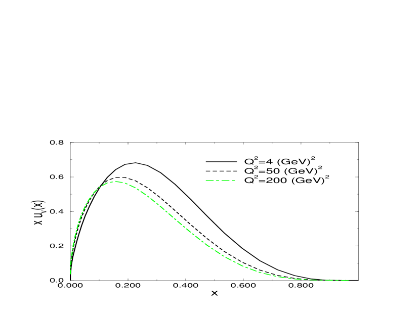
Figure 1: Evolution of the unpolarized valence quark distributions ${x\rm u_{v}}$ versus x for various $Q^{2}$ values

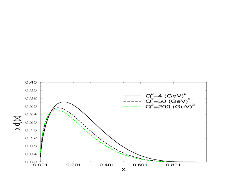
Figure 2: Unpolarized ${x\rm d_{v}}$ versus x for various $Q^{2}$ values

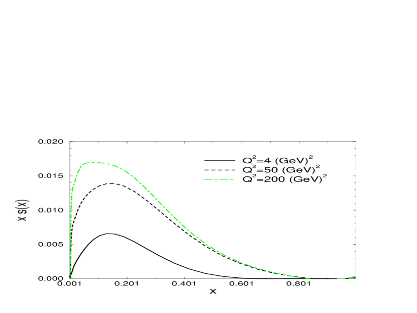
Figure 3: Unpolarized ${x\rm s}$ distribution versus x for various $Q^{2}$ values

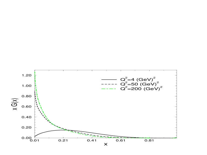
Figure 4: Unpolarized gluon distribution ${x\rm G}$ versus x for various $Q^{2}$ values

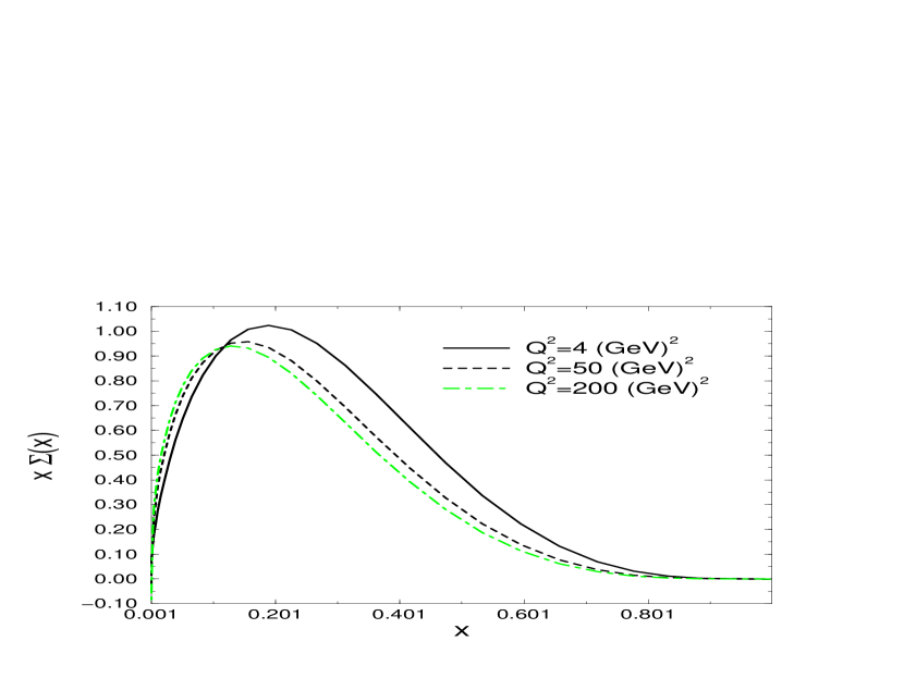
Figure 5: Unpolarized $x\Sigma=x(u+d+s)$ versus x for various $Q^{2}$ values

Figure 6: Longitudinally polarized ${x\rm\Delta u_{v}}$, plotted versus x, for various $Q^{2}$ values

Figure 7: Longitudinally polarized ${x\rm\Delta d_{v}}$ versus x for various $Q^{2}$ values

Figure 8: Longitudinally polarized ${x\rm\Delta s}$ versus x for various $Q^{2}$ values

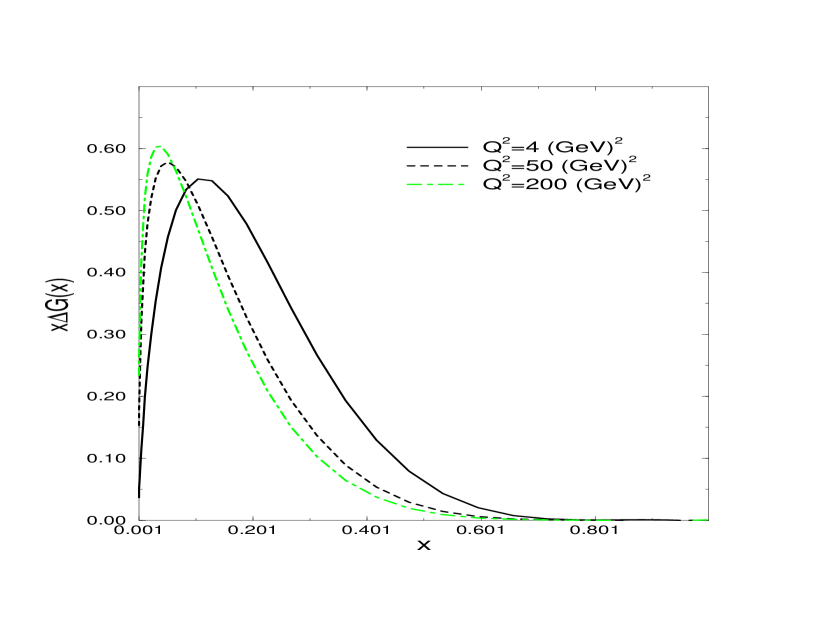
Figure 9: Longitudinally polarized ${x\rm\Delta G}$ versus x, shown for various $Q^{2}$ values

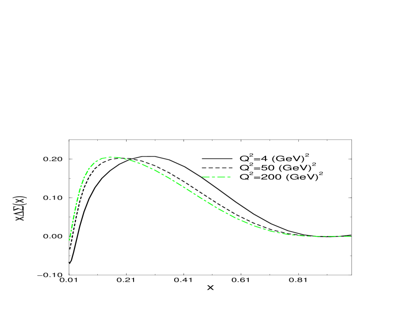
Figure 10: Longitudinally polarized $x\Delta\Sigma$ versus x, shown for various $Q^{2}$ values

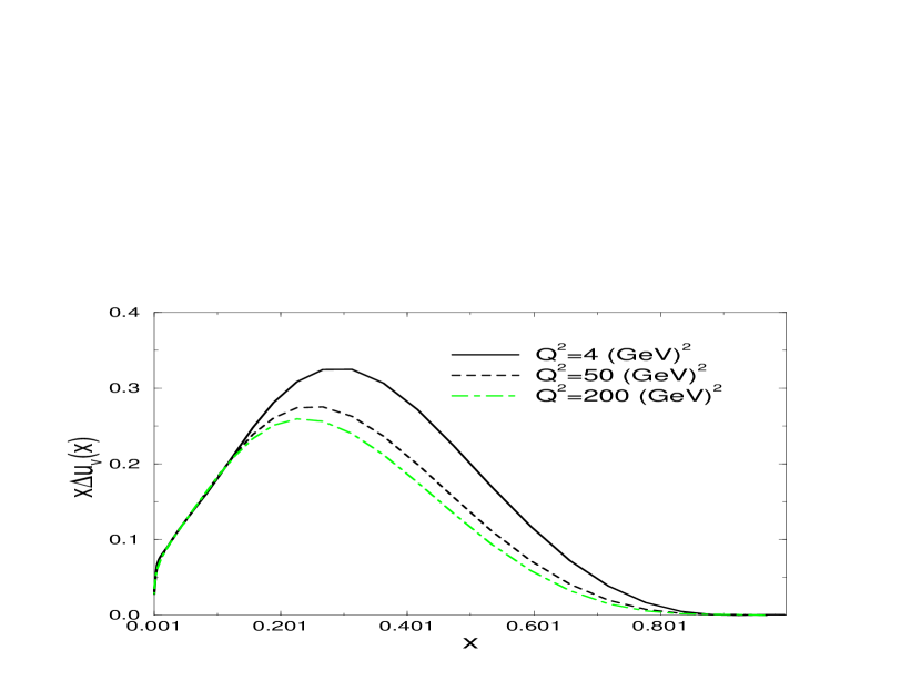
Figure 11: Transversely polarized ${x\rm\Delta_{T}u_{v}}$ versus x, shown for various $Q^{2}$ values

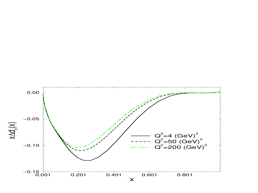
Figure 12: Transversely polarized ${x\Delta_{T}d_{v}}$ versus x, shown for various $Q^{2}$ values

Figure 13: Transversely polarized ${\rm x\Delta_{T}s}$, versus x, shown for various $Q^{2}$ values

11 Appendix. List of all the NLO polarized kernels

The references for the unpolarized NLO kernels are [2, 3]. The longitudinally polarized kernels can be found either as anomalous dimensions or splitting functions in [13, 14] The Perturbative expansion of the kernels is

$$\Delta P_{ij}(x,\alpha_{s})=\left({\alpha_{s}\over 2\pi}\right)\Delta P^{(0)}_{ij}(x)+\left({\alpha_{s}\over 2\pi}\right)\Delta P^{(1)}_{ij}(x)+...$$ (3)

where $ij$ are flavour indices. The non-singlet and the singlet polarized LO kernels, respectively, are given by

$$\Delta P^{(0)}_{NS}(x)=P^{(0)}_{qq}(x)=C_{F}\left({2\over(1-x)_{+}}-1-x+{3\over 2}\delta(1-x)\right)$$

$$\Delta P^{(0)}_{qq}(x)=\Delta P^{(0)}_{NS}(x)$$

$$\Delta P^{(0)}_{qg}(x)=2n_{f}T_{R}(2x-1)$$

$$\Delta P^{(0)}_{gq}(x)=C_{F}(2-x)$$

$$\Delta P^{(0)}_{gg}(x)=2C_{G}\left({1\over(1-x)_{+}}-2x+1\right)+{\beta_{0}\over 2}\delta(1-x).$$ (4)

The “+” distributions are defined by

$$\int_{0}^{1}dx{f(x)\over(1-x)_{+}}=\int_{0}^{1}dx{f(x)-f(1)\over 1-x}.$$ (5)

The non-singlet NLO kernels are given by

$$\Delta P^{(1)}_{NS\pm}=C_{F}^{2}\left[P_{F}(x)\mp P_{A}(x)+\delta(1-x)\left({3\over 8}-{\pi^{2}\over 2}+6\zeta(3)\right)\right]$$

$$\hskip 56.9055pt+{1\over 2}C_{F}C_{A}\left[P_{G}(x)\pm P_{A}(x)+\delta(1-x)\left({17\over 12}+{11\over 9}\pi^{2}-6\zeta(3)\right)\right]$$

$$\hskip 56.9055pt+C_{F}T_{R}n_{f}\left[P_{N_{F}}(x)-\delta(1-x)\left({1\over 6}+{2\over 9}\pi^{2}\right)\right]$$

$$P_{F}(x)=-2{1+x^{2}\over 1-x}\ln x\ln(1-x)-\left({3\over 1-x}+2x\right)\ln x-{1\over 2}(1+x)\ln^{2}x-5(1-x)$$

$$P_{A}(x)=2\left({1+x\over 1+x^{2}}\right)S_{2}(x)+2(1+x)\ln x+4(1-x)$$

$$P_{G}(x)={1+x^{2}\over(1-x)_{+}}\left[\ln^{2}x+{11\over 3}\ln x+{67\over 9}-{\pi^{2}\over 3}\right]+2(1+x)\ln x+{40\over 3}(1-x)$$

$$P_{N_{F}}(x)={2\over 3}\left[{1+x^{2}\over(1-x)_{+}}\left(-\ln x-{5\over 3}\right)-2(1-x)\right]$$

where

$$S_{2}(x)=-2{\it Li}_{2}(-x)-2\ln x\ln(1+x)+{1\over 2}\ln^{2}x-{\pi^{2}\over 6}.$$ (8)

The NLO polarized singlet kernels are given by

$$\Delta P^{(1)}_{qq}(x)=\Delta P^{(1)}_{NS+}+2C_{F}T_{R}n_{f}\Delta F_{qq}$$

$$\Delta P^{(1)}_{qg}(x)=C_{F}n_{f}T_{R}\Delta F^{(1)}_{qg}(x)+C_{G}n_{f}T_{R}\Delta F^{(2)}_{qg}(x)$$

$$\Delta P^{(1)}_{gq}(x)=C_{F}n_{f}T_{R}\Delta F^{(1)}_{gq}(x)+C_{F}^{2}F^{(2)}_{gq}(x)+C_{F}C_{G}\Delta F^{(3)}_{gq}(x)$$

$$\Delta P^{(1)}_{gg}(x)=-C_{G}T_{R}n_{f}\Delta F^{(1)}_{gg}(x)-C_{F}T_{R}n_{f}\Delta F^{(2)}_{gg}(x)+C_{G}^{2}\Delta F^{(3)}_{gg}(x)$$ (9)

where $C_{G}=C_{A}=N_{c}$ and

$$\Delta F_{qq}(x)=1-x-(1-3x)\ln x-(1+x)\ln^{2}x$$

$$\Delta F^{(1)}_{qg}(x)=-22+27x-9\ln x+8(1-x)\ln(1-x)$$

$$\hskip 56.9055pt+\delta p_{qg}(x)\left[2\ln^{2}x(1-x)-4\ln(1-x)\ln x+\ln^{2}x-{2\over 3}\pi^{2}\right]$$

$$\Delta F^{(2)}_{qg}(x)=2(12-11x)-8(1-x)\ln(1-x)+2(1+8x)\ln x$$

$$\hskip 56.9055pt-2\left[\ln^{2}(1-x)-{\pi^{2}\over 6}\right]\delta p_{qg}(x)-\left[2S_{2}(x)-3\ln^{2}x\right]\delta p_{qg}(-x)$$

$$\Delta F^{(1)}_{gq}(x)=-{4\over 9}(x+4)-{4\over 3}\delta p_{gq}(x)\ln(1-x)$$

$$\Delta F^{(2)}_{gq}(x)=-{1\over 2}-{1\over 2}(4-x)\ln x-\delta p_{gq}(-x)\ln(1-x)+\left[-4-\ln^{2}(1-x)+{1\over 2}\ln^{2}x\right]\delta p_{qg}(x)$$

$$\Delta F^{(3)}_{gq}(x)=(4-13x)\ln x+{1\over 3}(10+x)\ln(1-x)+{1\over 9}(41+35x)+{1\over 2}\left[-2S_{2}(x)+3\ln^{2}x\right]\delta p_{gq}(-x)$$

$$\hskip 56.9055pt+\left[\ln^{2}(1-x)-2\ln(1-x)\ln x-{\pi^{2}\over 6}\right]\delta p_{gq}(x)$$

$$\Delta F^{(1)}_{gg}(x)=4(1-x)+{4\over 3}(1+x)\ln x+{20\over 9}\delta p_{gg}(x)+{4\over 3}\delta(1-x)$$

$$\Delta F^{(2)}_{gg}=10(1-x)+2(5-x)\ln x+2(1+x)\ln^{2}x+\delta(1-x)$$

$$\Delta F^{(3)}_{gg}(x)={1\over 3}(29-67x)\ln x-{19\over 2}(1-x)+4(1+x)\ln^{2}x-2S_{2}(x)\delta p_{gg}(-x)$$

$$\hskip 56.9055pt+\left[{67\over 9}-4\ln(1-x)\ln x+\ln^{2}x-{\pi^{2}\over 3}\right]\delta p_{gg}(x)+\left[3\zeta(3)+{8\over 3}\right]\delta(1-x),$$ (10)

with

$$\delta p_{qg}(x)=2x-1$$

$$\delta p_{gq}(x)=2-x$$

$$\delta p_{gg}(x)={1\over(1-x)_{+}}-2x+1.$$ (11)

The unpolarized kernels, to LO are given by

$$P^{(0)}_{qq,NS}=\Delta P^{(0)}_{NS}$$ (12)

for the non-singlet sector, and by

$$P^{(0)}_{qq}(x)=P^{(0)}_{qq,NS}$$

$$P^{(0)}_{qg}(x)=2T_{R}n_{f}\left(x^{2}+(1-x)^{2}\right)$$

$$P^{(0)}_{gq}(x)=C_{F}{1+(1-x)^{2}\over x}$$

$$P^{(0)}_{gg}(x)=2N_{c}\left({1\over(1-x)_{+}}+{1\over x}-2+x(1-x)\right)+{\beta_{o}\over 2}\delta(1-x)$$ (13)

in the singlet sector.

The NLO unpolarized non-singlet and singlet kernels are given by

$$P^{(1)\pm}_{NS}(x)=\Delta P^{(1)\mp}_{NS}(x)$$ (14)

and

$$P^{(1)}_{qq}(x)=P^{(1)}_{NS+}+2C_{F}T_{R}n_{f}F_{qq}$$

$$P^{(1)}_{qg}(x)=C_{F}n_{f}T_{R}F^{(1)}_{qg}(x)+C_{G}n_{f}T_{R}F^{(2)}_{qg}(x)$$

$$P^{(1)}_{gq}(x)=C_{F}n_{f}T_{R}F^{(1)}_{gq}(x)+C_{F}^{2}F^{(2)}_{gq}(x)+C_{F}C_{G}F^{(3)}_{gq}(x)$$

$$P^{(1)}_{gg}(x)=C_{F}T_{R}n_{f}F^{(1)}_{gg}(x)+C_{G}T_{R}n_{f}F^{(2)}_{gg}(x)++C_{G}^{2}F^{(3)}_{gg}(x)$$

$$F_{qq}(x)={20\over 9x}-2+6x-{56\over 9}x^{2}+(1+5x+{8\over 3}x^{2})\ln x-(1+x)\ln^{2}x$$

$$F^{(1)}_{qg}=4-9x-(1-4x)\ln x-(1-2x)\ln^{2}x+4\ln(1-x)$$

$$+\left[2\ln^{2}\left({1-x\over x}\right)-4\ln\left({1-x\over x}\right)-{2\over 3}\pi^{2}+10\right]p_{qg}(x)$$

$$F^{(2)}_{qg}={182\over 9}+{14\over 9}x+{40\over 9x}+({136\over 3}x-{38\over 3})\ln x-4\ln(1-x)-(2+8x)\ln^{2}x$$

$$+\left[-\ln^{2}x+{44\over 3}\ln x-2\ln^{2}(1-x)+4\ln(1-x)+{\pi^{2}\over 3}-{218\over 9}\right]p_{qg}(x)$$

$$\hskip 28.45274pt+2p_{qg}(-x)S_{2}(x)$$

$$F^{(1)}_{gq}=-{4\over 3}x-\left[{20\over 9}+{4\over 3}\ln(1-x)\right]p_{gq}(x)$$

$$F^{(2)}_{gq}(x)=-{5\over 2}-{7\over 2}x+(2+{7\over 2}x)\ln x-(1-{1\over 2}x)\ln^{2}x-2x\ln(1-x)$$

$$-\left[3\ln(1-x)+\ln^{2}(1-x)\right]p_{gq}(x)$$

$$F^{(3)}_{gq}(x)=\left({28\over 9}+{65\over 18}x+{44\over 9}x^{2}-(12+5x+{8\over 3}x^{2}\right)\ln x+(4+x)\ln^{2}x+2x\ln(1-x)$$

$$\hskip 28.45274pt+\left[-2\ln x\ln(1-x)+{1\over 2}\ln^{2}x+{11\over 3}\ln(1-x)-{\pi^{2}\over 6}+{1\over 2}+\ln^{2}(1-x)\right]p_{gq}(x)$$

$$\hskip 28.45274pt+S_{2}(x)p_{gq}(-x)$$

$$F^{(1)}_{gg}(x)=-16+8x+{20\over 3}x^{2}+{4\over 3x}-(6+10x)\ln x-2(1+x)\ln^{2}x-\delta(1-x)$$

$$F^{(2)}_{gg}(x)=2-2x+{26\over 9}(x^{2}-{1\over x})-{4\over 3}(1+x)\ln x-{20\over 9}p_{gg}(x)-{4\over 3}\delta(1-x)$$

$$F^{(3)}_{gg}(x)={27\over 2}(1-x)+{67\over 9}(x^{2}-{1\over x})-({25\over 3}-{11\over 3}x+{44\over 3}x^{2})\ln x+4(1+x)\ln^{2}x$$

$$\hskip 28.45274pt+\left[{67\over 9}-4\ln x\ln(1-x)+\ln^{2}x-{\pi^{2}\over 3}\right]p_{gg}(x)+2p_{gg}(-x)S_{2}(x)$$

$$\hskip 56.9055pt+\delta(1-x)\left({8\over 3}+3\zeta(3)\right)$$ (16)

We have set

$$p_{qq}(x)={2\over(1-x)_{+}}-1-x$$

$$p_{qg}(x)x^{2}+(1-x)^{2}$$

$$p_{gq}(x)={1+(1-x)^{2}\over x}$$

$$p_{gg}(x)={1\over(1-x)_{+}}+{1\over x}-2+x(1-x)$$ (17)

The kernel for the transverse polarization is written as

$$\Delta_{T}P_{q^{\pm}}=\Delta_{T}P^{(0)}_{qq}(x)+{\alpha_{s}(Q^{2})\over 2\pi}\Delta_{T}P^{(1)}_{q^{\pm}}(x)$$ (18)

with the LO expression [16]

$$\Delta_{T}P_{q^{\pm}}=C_{F}\left[{2x\over(1-x)_{+}}+{3\over 2}\delta(1-x)\right].$$ (19)

The NLO corrections are given by [17]

$$\Delta_{T}P^{(1)}_{q^{(\pm)}}(x)=\Delta_{T}P^{(1)}_{qq}(x)\pm\Delta_{T}P^{(1)}_{q\bar{q}}(x),$$ (20)

$$\Delta_{T}P^{(1)}_{qq}(x)=C_{F}^{2}\left[1-x-\left({3\over 2}+2\ln(1-x)\right)\ln x\Delta_{T}P^{(0)}_{qq}(x)\right.$$

$$\left.+\left({3\over 8}-{\pi^{2}\over 2}+6\zeta(3)\right)\delta(1-x)\right]+{1\over 2}C_{F}C_{G}\left[-(1-x)+\left({67\over 9}+{11\over 3}\ln x+\ln^{2}x-{\pi^{2}\over 3}\right)\delta_{T}P^{(0)}_{qq}(x)\right.$$

$$\left.+\left({17\over 12}+{11\over 9}\pi^{2}-6\zeta(3)\right)\delta(1-x)\right]+{2\over 3}C_{F}T_{R}n_{f}\left[\left(-\ln x-{5\over 3}\right)\delta_{T}P^{(0)}_{qq}(x)-\left({1\over 4}+{\pi^{2}\over 3}\right)\delta(1-x)\right),$$

$$\Delta_{T}P^{(1)}_{q\bar{q}}(x)=C_{F}\left(C_{F}-{1\over 2}C_{G}\right)\left(-(1-x)+2S_{2}(x)\delta_{T}P^{(0)}(-x)\right).$$ (22)

References

- [1] G.P. Ramsey, Prog. Part. Nucl. Phys. 39 (1997) 599.
- [2] W. Furmanski and R. Petronzio, Nucl. Phys. B195 (1982) 237;
- [3] Z. Phys. C11 (1982) 293; Phys. Lett. 97B, (1980) 437.
- [4] Notice that eqs. (3.26) and (3.37) of [2] should read as in our eq. (43) and eq. (53) respectively.
- [5] M. Ropele, M. Traini and V. Vento, Nucl. Phys. A584 (1995) 634.
- [6] X. Song, J.S. McCarthy and H.J. Weber, hep/ph 9702363. H. Weber X. Song and M. Kirchbach, Mod. Phys. Lett. A12, (1997) 729.
- [7] N. Isgur and G. Karl, Phys. Rev. D 18 (1978) 4187; D19 (1979) 2653.
- [8] A.V. Efremov and A.V. Radyushkin, Theor. Math. Phys. 42 (1980) 97; Phys. Lett. B94 (1980) 245; S.J. Brodsky and G.P. Lepage, Phys. Lett. B 87 (1979) 359; Phys. Rev. D22 (1980) 2157.
- [9] X. Ji, Phys. Rev. D55 (1997) 7114; A.V. Radyushkin Phys. Rev. D56 (1997).
- [10] M. Hirai, S. Kumano, M. Miyama, Comput.Phys.Commun.108 (1998) 38; J. Blümlein, B. Geyer and D. Robaschik, hep-ph/9711405. M. Miyama, S. Kumano, hep-ph/9508246.
- [11] R. Kobayashi, M. Konuma, S. Kumano, Comput.Phys.Commun.86:264-278,1995.
- [12] G. Curci, W. Furmanski and R. Petronzio, Nucl. Phys. B175 (1980) 27.
- [13] R. Mertig and W. L. Van Neerven, Z.Phys.C70:637-654,1996.
- [14] W. Vogelsang, Nucl.Phys.B475:47-72,1996.
- [15] S. Chang. C. Corianò, R. D. Field and L. E. Gordon, hep-ph/9705249, to appear on Nucl. Phys. B; Phys. Lett. B403 (1997) 344.
- [16] X. Artru and M. Mekhfi, Z. Phys. C45 (1990) 669.
- [17] S. Kumano and M Miyama, Phys. Rev. D56 (1997) 2504; A. Hayashigaki, Y. Kanazawa and Y. Koike, hep-ph/9707208; W. Vogelsang, hep-ph/9706511.
- [18] G. Ramsey, Journ. of Comput. Phys. 60, (1985) 119.
- [19] S. Cotanch, unpublished.
- [20] T. Gehrmann and W.J. Sterling, Z.Phys.C65:461-470,1995.
- [21] D. Heddle, Y. R. Kwon and F. Tabakin, Comp. Phys. Comm. 38 (1985) 71.
- [22] Y.R. Kwon, F. Tabakin, Phys. Rev. C 18 (1978) 932.
- [23] J.P. Ralston and D.E. Soper, Nucl. Phys. B152 (1979) 109.
- [24] R.L. Jaffe and X. Ji, Phys. Rev. Lett. 67 (1991) 552;
- [25] H.L. Lai et al, Phys. Rev. D55, (1997) 1280; Phys. Rev. D51 (1996) 4763; W.K. Tung hep-ph/9608293.