Quark distribution in the pion within the instanton liquid model

Abstract

The leading-twist valence-quark distribution function in the pion is obtained at a low normalization scale of an order of the inverse average size of an instanton $\rho_{c}$. The momentum dependent quark mass and the quark-pion vertex are constructed in the framework of the instanton liquid model, using a gauge invariant approach. The parameters of instanton vacuum, the effective instanton radius and quark mass, are related to the vacuum expectation values of the lowest dimension quark-gluon operators and to the pion low energy observables. An analytic expression for the quark distribution function in the pion for a general vertex function is derived. The results are QCD evolved to higher momentum-transfer values, and reasonable agreement with phenomenological analyzes of the data on parton distributions for the pion is found.

1 Introduction

Hadron structure functions, in terms of quark and gluon distributions specifying the fraction $xp$ of the initial hadron momentum $p$ carried by the active parton, play an important role in QCD inclusive processes. Although the evolution of parton distributions at sufficiently large virtuality $Q^{2}$ is controlled by the renormalization scale dependence of twist-2 quark and gluon operators within QCD perturbation theory, the derivation of the parton distributions themselves at an initial $Q^{2}$ value from first principles still remains a challenge. Hence, central predictions unknown in QCD are parton distributions at relatively low virtuality determined in a nonperturbative scheme.

There is some recent progress in the calculation of moments of the pion and $\rho-$ meson parton distributions [1] within the lattice QCD (LQCD) using Wilson fermions in the quenched approximation, where internal quark loops are neglected. These LQCD predictions for the moments of the pion distribution function confirm the results of previous analyzes [2], being also in qualitative agreement with that extracted phenomenologically[3, 4] from experiment[5]. However, the calculated moments are still of a relatively low accuracy. Besides, only a few lowest-order moments are available, while the reconstruction of the $x$-dependent distributions needs, in principle, the knowledge of all moments. Furthermore, the QCD sum rules calculations of parton distributions in the pion are only moderately successful [6], the results being justified in a limited region of the scaling variable $x$.

Recently, the quark distribution function in the pion was obtained [7] in the framework of the Nambu - Jona - Lasinio (NJL) model [8]. These and similar studies are based on the assumption that the calculation of the twist-2 matrix elements, within the QCD inspired effective approaches, gives distributions at a low momentum scale $\mu_{0}\raisebox{-2.27621pt}{\hskip 2.84526pt$\stackrel{{\scriptstyle<}}{{\sim}}$\hskip 2.84526pt}1$ GeV, where such effective theories make sense. The distributions obtained are extrapolated to higher experimentally accessible momentum scales using perturbative QCD, so that comparison with experimental data can be made. However, the problem of the NJL model is that it is nonrenormalizable and thus, to avoid this defect, different ad hoc assumptions about momentum cutoff parameters are introduced.

The instanton model of the QCD vacuum (for recent review see , e.g., [9, 10]), which gives the dynamical mechanism of chiral symmetry breaking and provides the solution of the $U_{A}(1)$ problem[11], describes well the properties of pion [12, 13, 14] and kaon [15]. Moreover, it dynamically generates the momentum-dependent effective quark mass $M_{q}$ and quark-pion vertex $g_{\pi qq}$, and, as a consequence, provides inherently a natural ultraviolet cutoff parameter in the quark loop integrals through the effective instanton size $\rho_{c}$. On these grounds, one may believe that the instanton vacuum framework represents an important advance with respect to NJL-type models. The first attempt to calculate the pion structure function within the instanton model has been made in [16]. More recently, important progress has been achieved [17, 18] in calculating quark distributions in the nucleon within instanton-inspired approaches.

In the present paper, based on the quark-pion dynamics in the framework of the instanton liquid model, we calculate the leading-twist valence-quark distribution in the pion at a low normalization point of the order of the inverse average instanton size $\rho_{c}$. The calculations are performed in a gauge-invariant manner by taking into account $P-exp$ factor explicitly in the definition of nonlocal quantities [19, 20] and gauging the nonlocal quark - pion interaction[21, 22]. The momentum dependent quark mass and quark - pion vertex are constructed. The parameters of the instanton vacuum, effective instanton radius and quark mass, are related to the vacuum expectation values (VEV) of the lowest dimension quark-gluon operators and to the pion low energy observables. We derive the quark distribution in the pion and all its moments for the general form of the effective quark - pion vertex function. The validity of the isospin and total momentum parton sum rules is ensured by the pion compositeness condition[23], and it is consistent with the gauge invariant approach. As the effective instanton model is valid for values of the quark relative momentum up to $p\sim\rho_{c}^{-1}\approx 0.5-1$ GeV, the parton distributions calculated here are defined at this (low) normalization point $\mu_{0}\sim\rho_{c}^{-1}$. The results are QCD evolved to higher momentum-transfers, and we found reasonable agreement with phenomenological analyzes of the data on the pion distribution function.

The paper is organized as follows. In Sect. 2, we briefly outline the instanton liquid model and introduce the quark-pion vertex. In Sects. 3 and 4, the parameters of the instanton vacuum model are related to the vacuum expectation values of the lowest dimension quark-gluon operators and to the pion low energy observables. Then, we derive the expressions for the moments of the pion distribution (Sect. 5) and for the $x$-dependent distribution itself (Sect. 6), followed by the QCD evolution to higher values of the momentum transfer. In the last section, the results are discussed.

2 The instanton liquid model and the quark-pion vertex

We start with the nonlocal, chirally invariant Lagrangian of the instanton liquid model[9, 10], which describes the soft quark fields with the soft gluon fields being integrated out. The corresponding action for quarks interacting through the ’t Hooft vertices[11] can be expressed in a form similar to that of the NJL model

$$S_{inst}=\int d^{4}x\ \bar{q}(x)i\hat{\partial}q(x)+\int d^{4}xd^{4}x^{\prime}d^{4}yd^{4}y^{\prime}\ K(x,x^{\prime};y,y^{\prime})\cdot$$

$$\cdot\frac{1}{4(N^{2}_{c}-1)}\left\{\left[\frac{2N_{c}-1}{2N_{c}}\left(\bar{q}_{R}(x^{\prime})\tau^{a}q_{L}(x)\right)\left(\bar{q}_{R}(y^{\prime})\tau^{a}q_{L}(y)\right)+\right.\right.$$ (1)

$$\left.\left.+\frac{1}{8N_{c}}\left(\bar{q}_{R}(x^{\prime})\tau^{a}\sigma_{\mu\nu}q_{L}(x)\right)\left(\bar{q}_{R}(y^{\prime})\tau^{a}\sigma_{\mu\nu}q_{L}(y)\right)\right]+(R\leftrightarrow L)\right\}.$$

Here, $\tau^{a}=(1,i\vec{\tau})$ are the matrices for the flavor space, $N_{c}=3$ is the number of colors, and

$$q_{R(L)}(x)=\frac{1\pm\gamma_{5}}{2}q(x)$$

are the quark fields with definite chirality. In the following we neglect the current quark mass and restrict ourselves only by the nonstrange quark sector. In eq. (1), the kernel of the four-quark interaction $K(x,x^{\prime};y,y^{\prime})$ characterizes the region of the non-local quark-(anti)quark instanton induced interaction. It is dominated by the contribution of the zero mode quark wave functions in the field of (anti-)instanton:

$$K(x,x^{\prime};y,y^{\prime}) = \int dn(\rho)d^{4}zdU\left[\Big{(}i\hat{\partial}\varphi_{\rho}(x-z)\Big{)}\Big{(}i\hat{\partial}\varphi^{\dagger}_{\rho}(x^{\prime}-z)\Big{)}\right]\cdot$$ (2)

$$\cdot\left[\Big{(}i\hat{\partial}\varphi_{\rho}(y-z)\Big{)}\Big{(}i\hat{\partial}\varphi^{\dagger}_{\rho}(y^{\prime}-z)\Big{)}\right],$$

where $\varphi_{\rho}(x)$ is a quark zero mode profile function. In eq. (2), $n(\rho)$ denotes the density of instantons with size $\rho$, $z$ is the position of the instanton in the configuration space, and $dU$ is the color-space phase factor.

The spin-flavor structure of the action eq. (1) is invariant under the global axial $q(x)\to\exp{(i\gamma_{5}\tau\cdot\theta)}q(x)$ and vector transformations $q(x)\to\exp{(i\tau\cdot\theta)}q(x)$ and it anomalously violates the $U_{A}(1)$ symmetry: $q(x)\to\exp{(i\gamma_{5}\theta)}q(x)$. Within the instanton liquid model [24, 13, 14] it is argued that due to the long range instanton - anti-instanton interaction, configurations with large size instantons are strongly suppressed and the instanton density is sharply peaked at some finite average instanton size $\rho_{c}$ in the form $n(\rho)=n_{c}\delta(\rho-\rho_{c})$. Since the instanton liquid is assumed to be dilute, the mean separation between instantons is much larger than the average instanton size and the effective density $n_{c}$ is a small parameter of the approach. The values of $n_{c}$ and $\rho_{c}$ are estimated from the phenomenology of the QCD vacuum and hadron spectroscopy to be $n_{c}\sim 1\ fm^{-4}$, and $\rho_{c}$ changes within an interval $(1.5-2)\ GeV^{-1}$, where we put less restrictive limits on the range of values. It is important to note that the effective instanton size $\rho_{c}$, which defines the range of nonlocality, serves as a natural cutoff parameter of the effective low energy model. Moreover, the coupling constants of the model, eq. (2), are also expressed through the fundamental parameters describing the QCD instanton vacuum, $n_{c}$ and $\rho_{c}$. The model incorporates all attractive features of the NJL model and, at the same time, is free of arbitrariness in the choice of the ultraviolet cutoff procedure and physically all parameters are well understood. These peculiarities provide important advantages of the instanton model as compared to different versions of the NJL model (for a review, see, e.g., [8]).

The instanton induced interaction of quarks is responsible for strong spin-dependent forces in hadron multiplets[25]. In particular, this force is attractive for quark-antiquark states with vacuum and pion quantum numbers, repulsive for the singlet part of $\eta^{\prime}$, and absent (in the zero mode approximation) in the vector-like channels $\rho,\omega,$ etc. If the attraction is sufficiently large, it can rearrange the vacuum and bind a quark and an antiquark to form a light (Goldstone) meson state.

To study the formation of quark-antiquark bound states in the instanton liquid, it is convenient to rewrite the four-fermion term in the action eq. (1), linearizing the bilocals $\bar{q}(x)q(y)$ and $\bar{q}(x)\gamma_{5}\vec{\tau}q(y)$ by introducing the auxiliary composite meson fields $M(x)$[26] (mean field approximation) by virtue of the separability of the four-quark kernel. Then, we arrive at the following form of the effective nonlocal action corresponding to eq. (1):

$$S=S_{0}+S_{int},$$ (3)

where $S_{0}$ is the free action for quark and meson fields

$$S_{0}=\int d^{4}x\ \left\{\bar{q}(x)\ i\hat{D}q(x)+\frac{1}{2}\left[\sigma(x)(\Delta-m_{\sigma}^{2})\sigma(x)\right]+\frac{1}{2}\left[\vec{\pi}(x)(\Delta-m_{\pi}^{2})\vec{\pi}(x)\right]\right\},$$ (4)

and $S_{int}$ is the quark-meson interaction part

$$S_{int}= -\int d^{4}Xd^{4}x_{1}d^{4}x_{2}\ F(x_{1},x_{2};\mu_{0}^{2})\cdot$$

$$\cdot\bar{q}(X+x_{1})\ E(X+x_{1};X-x_{2})[M_{q}+g_{M\bar{q}q}(\Gamma\cdot T)M(X)]\ q(X-x_{2}),$$

with Dirac and isospin matrices for different meson states according to $\displaystyle(\Gamma\cdot T)_{\sigma}=I\cdot I,$ $\displaystyle(\Gamma\cdot T)_{\pi}=i\gamma_{5}\cdot\vec{\tau}$. In eq. (2), $g_{M\bar{q}q}$ is the quark-meson coupling constant and $M_{q}$ is the effective quark mass fixed in a gauge - invariant manner (see below) by the compositeness condition eq. (16) and the gap equation (17) in terms of the instanton density $n_{c}$ and the instanton size $\rho_{c}$. In Eqs. (4, 2) we neglect the terms induced by tensor interaction in eq. (1) since they do not contribute to the scalar channels.

To ensure the gauge invariance of the bilocal quark operators, which enters in Eqs. (3 - 2), with respect to external electromagnetic $A_{\mu}(z)$ and strong $A^{a}_{\mu}(z)$ gauge fields, we include into eq. (2), following [21], the path-ordered Schwinger phase factors

$$E(x;y)=E_{\gamma}(x;y)\cdot E_{g}(x;y),$$ (6)

$$E_{\gamma}(x;y)=P\ \exp\left\{-ieQ\int_{x}^{y}dz^{\mu}\ A_{\mu}(z)\right\},$$

$$E_{g}(x;y)=P\ \exp\left\{-ig\frac{\lambda^{a}_{c}}{2}\int_{x}^{y}dz^{\mu}\ A^{a}_{\mu}(z)\right\},$$

where the charge matrix is $Q=(1/3+\tau^{3}_{f})/2$, and the partial derivative $\partial_{\mu}$ is replaced by the covariant one $D_{\mu}=\partial_{\mu}-ieA_{\mu}-igA_{\mu}^{a}\lambda^{a}/2$. We adopt here that the integral in the exponent is evaluated along a straight line with $P$ being the path-ordering operator. The incorporation of a gauge - invariant interaction with gauge fields is of principal importance in order to treat correctly the hadron characteristics probed by external sources such as hadron form factors, structure functions, etc.

The Fourier transformed gauge-invariant nonlocal vertex function $\tilde{F}(k_{1},k_{2};\mu_{0}^{2})$ describes the amplitude of soft transition of a pion with momentum $p$ into a quark and an antiquark with momenta $k_{1}=p+k/2$ and $k_{2}=p-k/2$, respectively. This function represents the full interaction vertex with all quark-gluon excitations, harder than the scale $\mu_{0}\sim 1/\rho_{c}$, strongly (exponentially) suppressed. It is defined

$$F(k_{1},k_{2};\mu_{0}^{2})=\sqrt{\tilde{Q}(k_{1})\tilde{Q}(k_{2})}.$$ (7)

through the quark propagator $\tilde{Q}(p)$ normalized at zero to unity

$$\tilde{Q}(p)=\frac{1}{(2\pi)^{2}}\frac{p^{2}}{\rho_{c}^{2}}\int d^{4}x\ exp{(-ip\cdot x)}Q(x^{2}),\;\;\;(p=|p|)\;\;\;,$$ (8)

where

$$Q(x^{2})=\langle:\bar{q}(0)E_{g}(0,x)q(x):\rangle/\langle:\bar{q}(0)q(0):\rangle$$ (9)

is the normalized instanton induced nonperturbative part of the gauge invariant quark propagator in configuration space. Using the explicit expressions for the instanton field and quark zero mode the gauge-invariant quark propagator is given by [24, 19, 20]

$$Q(x^{2})=\frac{8\rho_{c}^{2}}{\pi}\int_{0}^{\infty}\ drr^{2}\int_{-\infty}^{\infty}\ dt\frac{\cos[\frac{r}{R}(\arctan(\frac{t+|x|}{R})-\arctan(\frac{t}{R}))]}{[R^{2}+t^{2}]^{3/2}[R^{2}+(t+|x|)^{2}]^{3/2}},$$ (10)

where $R^{2}=\rho_{c}^{2}+r^{2},~{}r=|\vec{z}|,~{}t=z_{4}$. In the derivation of these equations a reference frame is used, where the instanton is at the origin and $x^{\mu}$ is parallel to one of the coordinate axes, say $\mu=4$, serving as a “time” direction $({\it i.e.},\vec{x}=0,\ x_{4}=|x|)$. The propagator has the following expansions at small and large distances:

$$\displaystyle Q(x^{2})=\left\{\begin{array}[]{l}{1-{\displaystyle\frac{1}{4}}\frac{\displaystyle x^{2}}{\displaystyle\rho_{c}^{2}}+...\;\;\;{\rm as}\;\;\;x^{2}\to 0;}\\ {2\frac{\displaystyle\rho_{c}^{2}}{\displaystyle x^{2}}+...\;\;\;{\rm as}\;\;\;x^{2}\to\infty.}\end{array}\right.$$ (12)

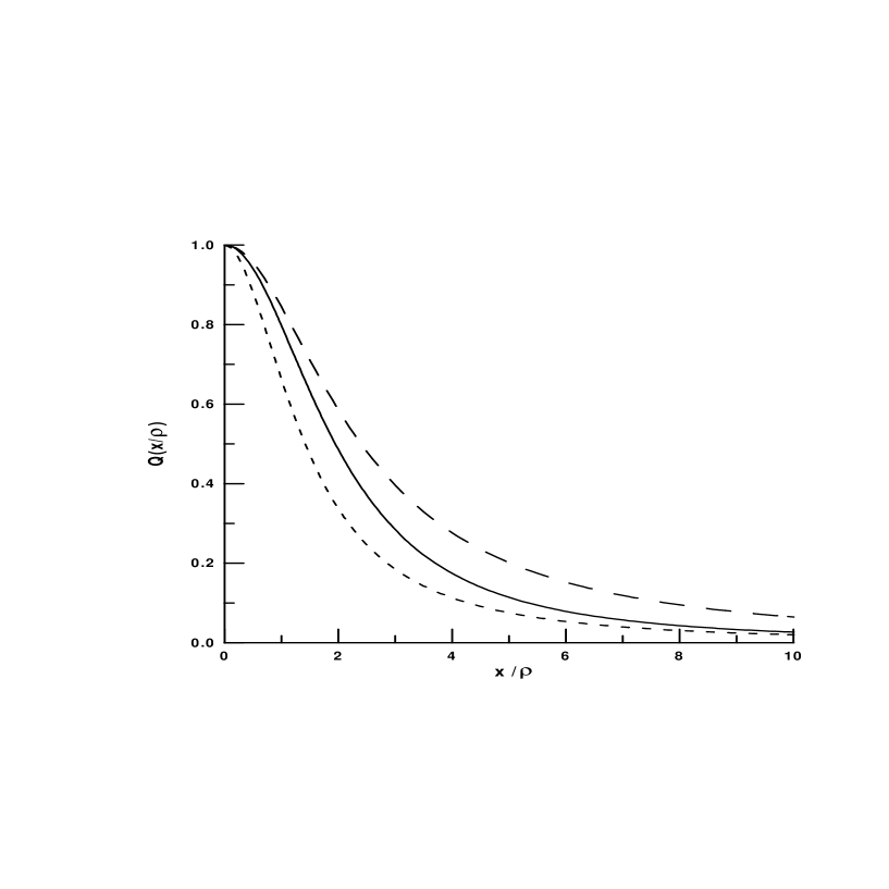
Figure 1: Configuration space representation of the normalized instanton induced nonperturbative part of the gauge-invariant quark propagator, eq.(10) (solid line); and the corresponding propagators derived without $P-exp$ factor in the singular (short-dashed) and regular, eq.(13), (long-dashed) gauges.

The gauge-invariant quark propagators in configuration and momentum representation are plotted in Figs. 1 and 2, respectively, along with the propagators derived in neglecting $P-exp$ factor in (9) and using the expressions for the quark zero mode in the singular and regular gauges. In the regular gauge, one has

$$Q_{reg}(x^{2})=\left.\frac{2}{y^{2}}\left(1-\frac{1}{\sqrt{1+y^{2}}}\right)\right|_{\displaystyle y=\frac{\displaystyle x}{\displaystyle 2\rho_{c}}}.$$ (13)

In the momentum representation, the normalized quark propagators (without $P-exp$ factor) are proportional to the square of the quark zero mode in the corresponding regular and singular gauges:

$$\tilde{Q}_{reg}(p) = \exp{(-2\rho_{c}p)}$$ (14)

$$\tilde{Q}_{sing}(p) = \left\{\left.z\frac{d}{dz}\left[I_{1}(z)K_{1}(z)-I_{0}(z)K_{0}(z)\right]\right|_{\displaystyle z=\frac{\displaystyle\rho_{c}p}{\displaystyle 2}}\right\}^{2}.$$ (15)

From Fig. 2, one can observe that in the momentum representation the shape of the propagator is very sensitive to the $P-exp$ factor .

One of the advantages of using the gauge - invariant formalism is that the parameters of the model, such as the size of instantons and the effective quark mass, gain physical meaning. As a consequence, all other physical quantities expressed through these parameters become automatically gauge - invariant ones. Moreover, they could be compared with those calculated in the lattice QCD, QCD sum rules or other QCD inspired approaches. In contrast, when one deals with noninvariant - gauge objects there can be chosen any convenient gauge.  It is most correct to consider the instanton vacuum field in the singular gauge and to construct the effective action in this specific gauge [9, 10]. In the coordinate space in the singular gauge the instantons fall off rapidly enough to provide small overlaps of neighbor pseudoparticles and quasiclassical considerations are justified. But at the end the action has to be independent on the choice of the gauge, otherwise the form of the action and other observables look rather awkward. This explicitly gauge invariant form is suggested in Eqs. (1 - 2). Note also that the quark propagator, eq. (9), has a direct physical interpretation in the heavy quark effective theory of heavy-light mesons as it describes the propagation of a light quark in the color field of an infinitely heavy quark [24].

It is important to emphasize that the meson fields entering the action eq. (3) are renormalized and the field renormalization constants of composite mesons are set equal to zero,

$$Z_{M}=1-g^{2}_{Mq\bar{q}}\left.\frac{\partial{\Pi}_{M}(p^{2})}{\partial p^{2}}\right|_{p^{2}=-m^{2}_{M}}=0,$$ (16)

where $\Pi_{M}(p^{2})$ is the meson field polarization operator. This condition [23] fixes the couplings of meson fields to quarks, $g_{Mq\bar{q}}$, (see section 4) and is a consequence of the compositeness of hadron states manifesting themselves as poles in the quark-(anti)quark scattering amplitude. As we will see below, it is precisely this condition supplemented by the gauge - invariance of the effective action, given by eq. (3), that leads to the correct parton isospin and momentum sum rules in the model.

3 Dynamical quark mass and expectation values of quark-gluon operators

Due to the effect of spontaneous breaking of the chiral symmetry, the momentum dependent quark mass $M_{q}(k)$ is dynamically developed. It obeys the well-known gap equation[9, 14]

$$\int\frac{d^{4}k}{(2\pi)^{4}}\frac{M_{q}^{2}(k)}{k^{2}+M_{q}^{2}(k)}=\frac{n_{c}}{4N_{c}},$$ (17)

the solution of which has the form

$$M_{q}(k)=M_{q}\tilde{Q}(k).$$ (18)

Given the dynamical mass, the values of the quark condensate,

$$\langle\bar{q}q\rangle=-4N_{c}\int\limits\frac{d^{4}k}{(2\pi)^{4}}\frac{M_{q}(k)}{k^{2}+M_{q}^{2}(k)},$$ (19)

and the average quark virtuality in the vacuum [27],

$$\lambda_{q}^{2}\equiv\frac{\langle:\bar{q}D^{2}q:\rangle}{\langle:\bar{q}q:\rangle}=-\frac{4N_{c}}{\langle\bar{q}q\rangle}\int\limits\frac{d^{4}k}{(2\pi)^{4}}k^{2}\frac{M_{q}(k)}{k^{2}+M_{q}^{2}(k)},$$ (20)

can be found.  The average quark virtuality defines the derivative of the quark condensate and thus nonlocal property of it. One of the main suggestion of the QCD sum rule method [28] was that the local quark and gluon condensates dominate in the light hadron physics and introduction of higher dimensional corrections or even nonlocal condensates themselves [27] have not to change the standard results too much. Thus, at least for consistency of local and nonlocal QCD sum rules, the derivative (virtuality) value has to be relatively small.  Phenomenologically, there is rather fine QCD sum rule analysis of this value [29] where it has to be defined as $\lambda_{q}^{2}\approx 0.4\pm 0.2$ GeV². The LQCD calculation yields $\lambda_{q}^{2}=0.55\pm 0.05\ GeV^{2}$ [30]. Certainly, there is corrections from direct instantons to the QCD sum rule result, but they have not to change the result drastically. It would also be urgent if the LQCD estimation could be confirmed by new calculations. The ratio $\eta=M_{q}^{2}(\lambda_{q})/\lambda_{q}^{2}$ characterizes the diluteness of the instanton liquid vacuum. The smallness of $\eta$ means that the dynamically generated quark mass is not big enough essentially to modify the instanton vacuum.

For the moment, it is instructive to consider equations Eqs. (17 - 20), neglecting the term $M_{q}^{2}(k)$ compared to $k^{2}$ in the denominator of the integrands. This approximation is justified in the dilute liquid regime where $\langle k^{2}\rangle=\lambda^{2}_{q}>>M_{q}^{2}(\lambda_{q})$. The observed accuracy of such procedure is better than $20-30\%$ if $\eta<1$.  Then, from Eqs. (19) and (20), by using the explicit forms given in Eqs. (10), (8), (18), we have

$$\langle\bar{q}q\rangle=-\frac{N_{c}M_{q}}{2\pi^{2}{\rho_{c}}^{2}},\ \ \ \ \ \lambda_{q}^{2}=\frac{2}{{\rho_{c}}^{2}}.$$ (21)

The first relation, put in the form $\displaystyle M_{q}=-({2\pi^{2}}/{N_{c}}){{\rho_{c}}^{2}\langle\bar{q}q\rangle},$ coincides with the result obtained in ref. [31], where the effective quark mass has been defined in a system of small size instantons interacting with long wave vacuum fields. The coefficient in this relation is equal to the normalization factor of the momentum representation of the quark propagator. It turns out that this factor, which is equal to $(2\pi)^{2}$, as seen in Eq.(8), is the same which appears in the gauge-invariant propagator and also in the singular gauge propagator (without $Pexp$).

The second relation in eq. (21) has recently been obtained in ref.[20], where nonlocal properties of the quark condensate are studied within the instanton model. The same result was also obtained in ref. [32] from direct calculations of the local mixed quark-gluon condensate in the framework of the Diakonov - Petrov model:

$$\frac{\lambda_{q}^{2}}{2}=\frac{\displaystyle\langle:\bar{q}(ig\sigma_{\mu\nu}G_{\mu\nu}^{a}\frac{\lambda^{a}}{2})q:\rangle}{\displaystyle\langle:\bar{q}q:\rangle}.$$ (22)

It is clear, from the expressions for the average quark virtuality, that the range of the quark - antiquark interaction is characterized by the effective size $\rho_{c}$ of the instanton fluctuations in the QCD vacuum. The natural gauge - invariant definition for the average quark virtuality, eq. (20) (and also that in eq. (19) for the quark condensate), with $M_{q}(k)$ defined in Eqs. (8) and (18), is valid only if the zero mode solution in eq. (8) is written in the gauge-invariant way. If we substituted its expression in the singular gauge (in neglecting $Pexp$ factors) in eq. (20), we would obtain $\lambda_{q}^{2}=9/(2\rho_{c}^{2})$, with a coefficient far from the correct one.

Inverting the relations eq. (21), we express the parameters of the instanton vacuum model in terms of the fundamental parameters of QCD vacuum ${\rho_{c}}^{2}={2}/{\lambda_{q}^{2}},$ $M_{q}=-({4\pi^{2}}/{N_{c}})({\langle\bar{q}q\rangle}/{\lambda_{q}^{2}}).$ If we expected “standard” values for the quark condensate, $\langle~{}\bar{q}q\rangle\approx-(230\ \mbox{MeV})^{3}$ (see, e.g., [10]), and for the average quark virtuality, $\lambda_{q}^{2}\approx 0.5\ GeV^{2}$ [29, 30], we would obtain $\rho_{c}^{-1}\approx 0.5$ GeV and $M_{q}\approx 0.32$ GeV. As we will see in the next section, the joined analysis of the vacuum and pion properties confirms this estimation.

Within the dilute liquid approximation, the gap equation, (17), leads to

$$n_{c}=\frac{N_{c}M_{q}^{2}\lambda^{2}_{q}}{4\pi^{2}}I_{n},\;\;\;{\rm with}\;\;\;I_{n}=\int_{0}^{\infty}duu\tilde{Q}^{2}(u/\rho_{c})\approx 0.61,$$ (23)

where the constant $I_{n}$ is independent of $\rho_{c}$. There are other different useful combinations relating vacuum parameters with each other. For example,

$$\langle\bar{q}q\rangle=-\frac{1}{I_{n}}\frac{n_{c}}{M_{q}}=-\frac{1}{2\pi\sqrt{I_{n}}}\sqrt{N_{c}n_{c}\lambda_{q}^{2}}.$$ (24)

These relations have the same parametric dependence as in the estimations obtained in [24, 10] but with different coefficients. The first one expresses the quark condensate in terms of the effective single instanton contribution times the density of instantons. The reason for the difference in the coefficients is that in [24], where it looks as $\displaystyle\langle\bar{q}q\rangle=-{n_{c}}/{M_{q}}$, the expressions were obtained from the instanton formula in the gas approximation by ad hoc replacing the current quark mass by the effective quark mass. In contrast, in deriving eq. (24) this replacing procedure is fixed by the gap equation eq. (17), with a definite coefficient mainly defined by the slope of the form factor $M_{q}(k)$. The second relation represents a self-consistent value of the quark condensate in the instanton vacuum model (cf. [10]). Further, since the instanton contribution to the value of the gluon condensate is given by: $\displaystyle\langle\frac{\alpha_{s}}{\pi}G^{2}\rangle|_{inst}=8n_{c}$, it can be expressed through the quark condensate and the average quark virtuality

$$\langle\frac{\alpha_{s}}{\pi}G^{2}\rangle|_{inst}=\frac{2^{5}\pi^{2}I_{n}}{N_{c}}\frac{\langle\bar{q}q\rangle^{2}}{\lambda_{q}^{2}}\raisebox{-2.27621pt}{\hskip 2.84526pt$\stackrel{{\scriptstyle<}}{{\sim}}$\hskip 2.84526pt}0.019\ GeV^{4}.$$ (25)

The “standard” value of the gluon condensate estimated in the original work, in ref. [28], was $\displaystyle\langle({\alpha_{s}}/{\pi})G^{2}\rangle\simeq 0.012$ GeV⁴. The latest reanalysis [33] of the QCD sum rules for heavy and light mesons and also recent lattice results [34] provide values which are twice or even larger than the “standard” one.

4 Pion low energy observables

Let us now consider the low-energy observables of the pion. The pion - quark coupling constant is determined by the compositeness condition, eq. (16), with the pion mass operator being

$$\Pi_{\pi}(p^{2})=N_{c}\int\frac{d^{4}k}{(2\pi)^{4}}\tilde{F}^{2}(k,k+p;\mu_{0}^{2})Tr\{\gamma_{5}S(k+p)\gamma_{5}S(k)\},$$ (26)

where the normalized nonlocal vertex is given in (7) and the quark Green function is $\displaystyle S(k)=[{M}_{q}\tilde{Q}(k)+\hat{k}]^{-1}$ with $\tilde{Q}(k)$ defined in (8).

From the definition eq. (16) we derive the expression for the pion - quark coupling constant $g_{\pi q\bar{q}}$

$$g_{\pi q\bar{q}}^{2}=\frac{2\pi^{2}}{N_{c}I_{g\pi}(-m_{\pi}^{2})}.$$ (27)

In the case of a massless pion, the integral $I_{g\pi}$ reduces to

$$I_{g\pi}(0)=\int\limits_{0}^{\infty}\frac{dk\ k^{3}\tilde{Q}(k)}{D^{2}(k)}\left[1-\frac{k}{4}\frac{\tilde{Q}^{\prime}(k)}{\tilde{Q}(k)}+\left(\frac{k}{4}\frac{\tilde{Q}^{\prime}(k)}{\tilde{Q}(k)}\right)^{2}\right],$$ (28)

where

$$\tilde{Q}^{\prime}(k)=\frac{d}{dk}\tilde{Q}(k),\;\;\;\;D(k)=M_{q}^{2}\tilde{Q}^{2}(k)+k^{2}.$$ (29)

The expression for $g_{\pi q\bar{q}}$ given in Eqs. (27) and (28) agrees with that derived in [14].

To fix the parameters in the instanton model, we consider the low energy decay constants of the pion. As it has recently been shown in [22], in the presence of nonlocal separable interaction the axial current conserved in the chiral limit can be constructed from the action eq. (1) by using a Noether - like method. The full current is the sum of local,

$$j^{\mu a}_{5(loc)}(x)=\frac{1}{2}\bar{q}(x)\gamma^{\mu}\gamma_{5}\tau^{a}q(x),$$ (30)

and nonlocal,

$$j^{\mu a}_{5(nl)}(x)= \int\prod_{i=1}^{4}dx_{i}\ K(x_{1},x_{2},x_{3},x_{4})\{A_{1}(x_{1},x_{2},x_{3},x_{4})\bar{q}(x_{1})i\gamma_{5}\tau^{a}q(x_{3})\bar{q}(x_{2})q(x_{4})+$$ (31)

$$+A_{2}(x_{1},x_{2},x_{3},x_{4})i\varepsilon^{abc}\bar{q}(x_{1})\tau^{c}q(x_{3})\bar{q}(x_{2})i\gamma_{5}\tau^{b}q(x_{4})\}$$

pieces. The coefficients $A_{1}$ and $A_{2}$ are derived in ref. [22] and in principle depend on the gauge fixing procedure. Fortunately, there is no path dependence for the longitudinal components of the current, and thus, the decay constants considered below are well-defined.

The axial and vector currents in different isospin states have a similar structure [22]. As a result, various Ward identities which follow from (partial) current conservation and the low-energy theorems are satisfied. In particular, the Goldberger - Treiman relation for the quark-pion coupling constant has the usual form

$$g_{\pi qq}=\frac{{M}_{q}}{f_{\pi}}$$ (32)

and the $\pi^{0}\rightarrow\gamma\gamma$ decay constant

$$g_{\pi\gamma\gamma}=\frac{1}{4\pi^{2}f_{\pi}}$$ (33)

is consistent with the requirement of axial anomaly.

We fix the model parameters to give the pion weak decay constant $f_{\pi}$, within 1% of accuracy.  In Table 1, we present the results. For the two model parameters, $M_{q}$ and $\rho_{c}$, we show the predictions for the quark-pion coupling $g_{\pi qq}$, the quark condensate $\langle\bar{q}q\rangle$, the average vacuum quark virtuality $\lambda_{q}^{2}$ and the instanton density $n_{c}$.

Table 1. The values of the low energy vacuum and pion observables discussed in the text.

$M_{q}$	$\rho_{c}$	$f_{\pi}$	$g_{\pi qq}$	$|\langle\bar{q}q\rangle|^{1/3}$	$\lambda_{q}^{2}$	$n_{c}$
(GeV)	(GeV-1)	(MeV)		(MeV)	(GeV2)	(fm-4)
0.18	1.0	92	3.7	294	2.2	1.56
0.22	1.5	92	5.5	233	1.0	0.86
0.23	1.7	93	6.2	215	0.83	0.70
0.26	2.0	91	7.7	197	0.63	0.57

As shown in Table 1, the values of the parameters $M_{q}$ and $\rho_{c}$ that reproduce the lowest dimension VEV with an accuracy of an order of $30\ \%$ are in the “window” $M_{q}=(220-260)$ MeV, $\rho_{c}=(1.5-2.0)$ GeV^-1. In the following we use the typical set of parameters:

$$M_{q}=230MeV,\ \ \ \ \ \rho_{c}=1.7\ GeV^{-1}.$$ (34)

The diluteness condition $\eta=M_{q}^{2}(\lambda_{q})/\lambda_{q}^{2}<<1$ is well satisfied within the whole “window”.

The momentum dependence of the vertices in the numerators of the integrands (which are defining physical quantities) is important because it provides the ultraviolet regularization. Also, due to momentum dependence of the vertices, the measure in the integrals looks like product of some powers of $k^{2}$ and the function $\tilde{Q}(k)$. This measure has maximum at $k^{2}$ of order $1/\rho_{c}^{2}$ and, at small momenta, the momentum dependent quark mass in denominators can be substituted by an effective constant mass parameter $m_{q}\approx M_{q}(k\sim\rho_{c}^{-1})$. With the form of momentum distribution shown in Fig. 2, it approximately equals to the mass at zero, $M_{q}(0)$. This mass parameter $m_{q}$ has to be identified with the standard constituent quark mass. Corresponding to this substitution, we redefine the function $D(k)$ given in eq. (29) as $D(k)=m_{q}^{2}+k^{2}$. The choice of the mass parameter,

$$m_{q}=230\ \mbox{MeV},$$ (35)

well reproduces the integrals defining the VEV given by Eqs. (17 - 20). This constant - mass approximation is often used in practice with the quark mass in the region $250-350$ MeV (see, f.i. [18, 35, 36]).

The model parameters and predictions for vacuum and pion observables are obtained within a set of approximations. We are working in the chiral limit of zero current quark mass. Further, within the zero mode approximation small contributions coming from vector mesons are neglected. Also only the lowest two - quark Fock intermediate state in the pion is taken into account, which corresponds to the quenched approximation. We regard that all these factors can change a little the numbers in Table 1, but the qualitative results discussed are not greatly influent.

5 Moments of the quark distribution function

The standard QCD analysis based on the Operator Product Expansion (OPE) relates moments of parton distributions at a given scale to the hadronic matrix elements of local twist-2 operators. This formalism is employed to separate the hard and soft parts of the forward scattering amplitude. Within the OPE, the hard part is calculable within perturbation theory in the form of Wilson coefficients. The soft part is represented by a set of local operators classified by the twist. Their matrix elements accumulate information on the nonperturbative structure of the QCD vacuum.

The twist-2 gauge - invariant non-singlet local quark operators with flavor $j$ are defined by

$$O_{\mu_{1}\mu_{2}..\mu_{N}}^{j}=i^{N}\bar{q}_{j}\{\gamma_{\mu_{1}}D_{\mu_{2}}..D_{\mu_{N}}\}_{S}q_{j},$$ (36)

where $D_{\mu}=\partial_{\mu}-igA^{a}_{\mu}\tau_{a}$ is the covariant derivative and the symbol $\{...\}_{S}$ means the traceless and symmetric part of the tensor. The matrix elements $A_{N}^{j}$ of the local operators $O_{N}^{j}$ between pion states $|\pi(p)\rangle$ with momentum $p$, renormalized at the normalization scale $\mu$, are defined by

$$A_{N}^{j}(\mu^{2})=\frac{i^{N}}{2}\langle\pi(p)|\bar{q}_{j}\hat{n}(n_{\nu}D^{\nu})^{N}q_{j}|\pi(p)\rangle|_{\mu},$$ (37)

where $n_{\nu}$ is a light-like vector, with $n^{2}=0$ and $(np)=1$, introduced to select the symmetric traceless part of the operator $O_{N}^{j}$, eq. (36). Let us now define the quark distribution for the $j-$th flavor in terms of its moments, viz.:

$$A_{N}^{j}(\mu^{2})=\int^{1}_{0}dx\ x^{N-1}q_{j}(x,\mu^{2}).$$ (38)

The $x-$variable is the fraction of the longitudinal pion momentum carried by a quark in the infinite-momentum frame. The $\mu^{2}$ dependence of $A^{j}_{N}$ is known exactly from the solution of the perturbative QCD evolution equations, while the nonperturbative dynamical model provides the initial input for this evolution. These initial values of the moments are calculated here in the instanton model, which specifies a low momentum transfer value related to the scale $\mu_{0}^{2}\propto 1/\rho_{c}^{2}$.

The $N-$th moment $A_{N}^{val}(\mu_{0}^{2})$ in the instanton model, from Eqs. (36 - 38), can be expressed as (see Fig. 3)

$$\displaystyle A_{N}^{val} (\mu_{0}^{2})p_{\mu_{1}}p_{\mu_{2}}..p_{\mu_{N}}=2N_{c}g_{\pi q\bar{q}}^{2}\int\frac{d^{4}k}{(2\pi)^{4}}\cdot$$

$$\cdot\left\{\tilde{F}^{2}(k,k+p;\mu_{0}^{2})Tr[\gamma_{5}S(k+p)\{\gamma_{\mu_{1}}(k+p)_{\mu_{2}}..(k+p)_{\mu_{N}}\}_{S}S(k+p)\gamma_{5}S(k)]-\right.$$

$$\left.-2\Big{[}\frac{\partial\tilde{F^{2}}(k,k+p;\mu_{0}^{2})}{\partial(k+p)^{2}}\Big{]}Tr[\gamma_{5}S(k+p)\{(k+p)_{\mu_{1}}(k+p)_{\mu_{2}}..(k+p)_{\mu_{N}}\}_{S}\gamma_{5}S(k)]\right\}.$$

Here, due to the nonlocal character of the interaction Eqs. (2 - 6), the additional term with a derivative ensures gauge invariance of the approach and enables us to satisfy the isospin and momentum conservation sum rules. Indeed, taking into account the compositeness condition eq. (16) we get for the first two moments

$$A_{1}^{val}(\mu_{0}^{2})=g_{\pi q\bar{q}}^{2}\cdot\left.\frac{\partial{\Pi}_{\pi}(p^{2})}{\partial p^{2}}\right|_{p^{2}=0}=1,\;\;A_{2}^{val}(\mu_{0}^{2})=\frac{g_{\pi q\bar{q}}^{2}}{2}\cdot\left.\frac{\partial{\Pi}_{\pi}(p^{2})}{\partial p^{2}}\right|_{p^{2}=0}=\frac{1}{2}.$$ (40)

The results for the first two moments, eq. (40), manifest the (normalization) isospin and momentum sum rules for the valence-quark distribution function as

$$\int^{1}_{0}dx\ q^{val}(x,\mu_{0}^{2})=1\;\;\;{\rm and}\;\;\;\int^{1}_{0}dx\ x[q^{val}(x,\mu_{0}^{2})+\bar{q}^{val}(x,\mu_{0}^{2})]=1,$$ (41)

where $\bar{q}^{val}(x)$ is the antiquark distribution. The fact that, at the low momentum scale $\mu_{0}$, the whole momentum in the pion is carried off by the valence quarks is due to the quenched approximation used, when only valence quark-antiquark intermediate states are included and all intrinsic quark-gluon sea states are neglected.

Thus, in the quenched approximation the dynamical information contained in the first two moments is strongly restricted by the symmetries and kinematics, and as a result, it is model independent. The nontrivial dynamics is contained in the moments with $N>2$. The general structure of the moments of the structure function (SF), from eq. (5), can be written in the form

$$A_{N}^{SF}(\mu_{0}^{2})=\frac{1}{2^{N-1}}\sum_{i=0}^{[\frac{N-1}{2}]}\frac{1}{2i+1}{N-1\choose 2i}J_{i}^{SF}(\mu_{0}^{2}),\ \ \ \ \ N=1,2,...$$ (42)

with the coefficients $J_{i}^{SF}$ given by

$$J_{i}^{SF}(\mu_{0}^{2})=\frac{1}{I_{g\pi}(0)}\left\{\int\limits_{0}^{\infty}\frac{dk\ k^{4i+3}\tilde{Q}(k)}{(k^{2}+m_{q}^{2})^{2i+3}}\Big{[}2k^{2}+(2i+3)m_{q}^{2}\Big{]}+...\right\},$$ (43)

where the vertex terms with derivatives, like that appearing in eq. (28) for $I_{g\pi}(0)$, are denoted by dots. In eq. (42), the square brackets $[...]$ mean the integer part of the number, and $\displaystyle{a\choose b}$ are the binomial coefficients.

It is instructive to consider two extreme cases, depending on the physics under consideration. If the QCD vacuum were a very dense medium, $\eta>>1$, then $J_{i}^{SF}=0$ for all $i$ except $i=0$. As a result, it leads to the set of moments $A_{N}=1/2^{(N-1)}$ for all $n$ and to a quark distribution which has the form of a delta function: $q(x)=\delta(x-1/2)$. This extreme case corresponds to the heavy quark limit, and the coefficients $J_{i}^{SF}$ represent consequent corrections in inverse powers of the heavy quark mass: $\displaystyle\sim(\langle k^{2}\rangle/m_{q}^{2})^{i}$. In the opposite extreme case of a very dilute vacuum $\eta<<1$ one gets $J_{i}^{SF}=1$ for all $i$ and $A_{N}=1/N$ for the moments. This extreme case corresponds to the momentum independent quark mass and provides flat quark distribution $q(x)=1$. Moreover, the first term in eq. (43) dominates over the terms indicated by dots, since the latter are small of an order of $O(\rho_{c}m_{q})$. A realistic situation seems to be somewhere in-between these two extremes. Note that the role of pion mass is negligible, but the interplay of the effective quark mass and the slope of the nonlocality in $\tilde{Q}(k)$ has an important effect.

6 Quark distribution function and its QCD evolution

Let us now turn our attention to the quark distribution itself. This distribution for the pion with 4-momentum $p$ is given by (see a graphical representation in Fig. 3)

$$q(x;\mu_{0}^{2})p^{\mu}=2N_{c}g^{2}_{\pi q\bar{q}}\int\frac{d^{4}k}{(2\pi)^{4}}\delta\big{[}x-1-(k\cdot n)\big{]}\cdot$$ (44)

$$\cdot Tr\left\{\gamma_{5}S(k+p)\left[\tilde{F}^{2}(k,k+p;\mu_{0}^{2})\gamma_{\mu}S(k+p)-2\left(\frac{\partial\tilde{F^{2}}(k,k+p;\mu_{0}^{2})}{\partial(k+p)^{2}}\right)(k+p)_{\mu}\right]\gamma_{5}S(k)\right\},$$

where $q(x)=\bar{u}(x)_{val}=d(x)_{val}$ for $\pi^{-}$. Here, we arrive at the quark distribution defined in a similar manner as that used in [37, 38]. The $\delta\big{[}x-1-(k\cdot n)\big{]}-$ function appearing in eq. (44) represents the effective vertex related to the composite operator $O_{N}^{j}$ given by eq. (36). It accumulates information about all moments of the distribution function (5) and is related to them by a Mellin transformation if the light-cone vector $n$ is normalized by $(pn)=1$. The light-cone vector $n$ serves to project out in Eqs. (5) and (44) symmetric traceless tensors. It can be easily shown that the first moments of $q(x)$ will reproduce the parton sum rules eq. (40).

To calculate the $k-$integral in eq. (44), we use $\alpha-$representation for the propagators,

$$\frac{1}{k^{2}+m^{2}}=\int\limits_{0}^{\infty}d\alpha\ \exp{\left[-\alpha(k^{2}+m^{2})\right]},$$ (45)

and for the vertex $\delta-$function,

$$\delta\big{[}x-(k\cdot n)\big{]}=\frac{1}{2\pi}\int\limits_{-\infty}^{\infty}d\alpha\ \exp{[i\alpha(x-k\cdot n)]}.$$ (46)

Then, a direct calculation from eq. (44) provides the result for the quark distribution, which in the massless case ($m_{\pi}^{2}=-p^{2}=0$) is reduced to

$$\displaystyle q(x,\mu_{0}^{2}) = \frac{N_{c}g^{2}_{\pi q\bar{q}}}{2\pi^{2}}\int\limits_{0}^{\infty}\int\limits_{0}^{\infty}d\nu_{1}d\nu_{2}\ F(\nu_{1})F(\nu_{2})\exp\Big{(}\frac{m_{q}^{2}}{\nu_{1}}+\frac{m_{q}^{2}}{\nu_{2}}\Big{)}\cdot$$

$$\cdot\left\{\left[E_{1}\left(\frac{m_{q}^{2}}{x\nu_{1}}\right)+\bar{x}\exp\left(-\frac{m_{q}^{2}}{x\nu_{1}}\right)\right]\Theta(\bar{x}\nu_{2}\geq x\nu_{1})+(x\leftrightarrow\bar{x})\right\}.$$

In the above equation, $\bar{x}=1-x$, $E_{1}(z)$ is the integral exponential, and $F(\nu)$ is the correlation function related to the vertex function $\tilde{Q}(k)$ by the Laplace transformation. The vertex $\tilde{Q}(p)$, in the essential region of $p$ ($0\leq p\leq 4/\rho_{c}$) is approximated by

$$\tilde{Q}(p)=4.5\exp{(-1.9\rho_{c}p)}-3.5\exp{(-3.6\rho_{c}p)},$$ (48)

which leads to the Laplace transform,

$$F(\nu)=\frac{\rho_{c}}{\sqrt{\pi}\sqrt{\nu}}\left[8.55\exp(-0.9\rho_{c}^{2}\nu)-12.6\exp(-3.24\rho_{c}^{2}\nu)\right].$$ (49)

Let us stress that the expressions eq. (42) for the moments and eq. (6) for the valence-quark distribution in the pion are universal ones and valid for any shape of the functions $\tilde{Q}(k)$ and $F(\nu)$, which in turn are determined by the concrete model of the quark-pion dynamics.

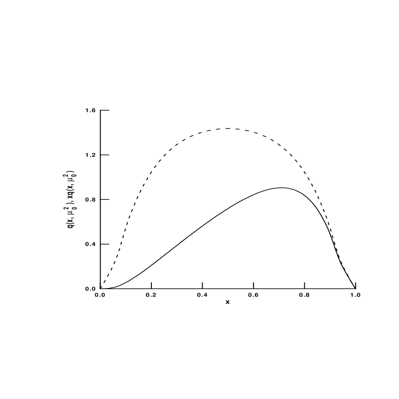
Figure 4: The valence-quark distribution function (DF) $q(x;\mu_{0}^{2})$ (dashed line) and the quark momentum distribution function (MDF) $xq(x;\mu_{0}^{2})$ (solid line) for the pion as a function of the longitudinal momentum fraction $x$ at the low momentum scale $\mu^{2}_{0}=0.19$ GeV² and density parameter ${\rho}_{c}m_{q}=0.39$.

The quark distribution $q(x,\mu_{0}^{2})$ and the momentum distribution (structure function) $xq(x,\mu_{0}^{2})$ are shown graphically in Fig. 4. We have to note that the shape of the distribution is quite stable with respect to changes of the instanton model parameters, if they are fixed to reproduce the pion low energy properties. We remind that we are computing only the leading-twist distributions at a low normalization point $\mu_{0}\sim\rho_{c}^{-1}$ rather than the full structure functions which contain also higher-twist corrections. The latter may be large at low $q^{2}$. We have also to note that these results differ strongly from those obtained in calculations with the NJL model [7] which yield distributions that are rather consistent with the strict chiral limit $q(x,\mu_{0}^{2})\approx 1$.

The computed distributions are then used as initial conditions for the perturbative evolution to higher values of $Q^{2}$, where the power corrections are expected to be suppressed, so that one can compare them with the available experimental data. Actually, we compare our theoretical predictions with the phenomenological analysis by Sutton et al [3] of the data taken from Drell - Yan and prompt photon experiments performed by the groups NA10 (CERN) and E615 (Fermilab) [5].

The form of the evolved distribution $q(x,Q_{0}^{2})$ at the momentum scale $Q_{0}^{2}=4$ GeV² is reconstructed from its moments evolved to this scale in the leading order (LO) and next-to -leading order (NLO) perturbative QCD in the $\overline{MS}$ scheme by using the first six Jacobi polynomials. To this goal we use the well-known expressions [39] for the perturbatively calculable coefficient function of the process $\displaystyle C_{i}^{N}=C_{0i}^{N}+\frac{\alpha_{s}(Q^{2})}{4\pi}C_{1i}^{N}$ and the anomalous dimensions $\gamma_{(n)}$ calculated up to LO and NLO. Thus, the final result for the moments obtained from the factorization procedure is

$$A_{N}(Q^{2})=\sum\limits_{i}C_{i}^{N}(Q^{2},\mu^{2})O_{i}^{N}(\mu^{2})=\int\limits_{0}^{1}dx\ x^{N}q(x,Q^{2}).$$ (50)

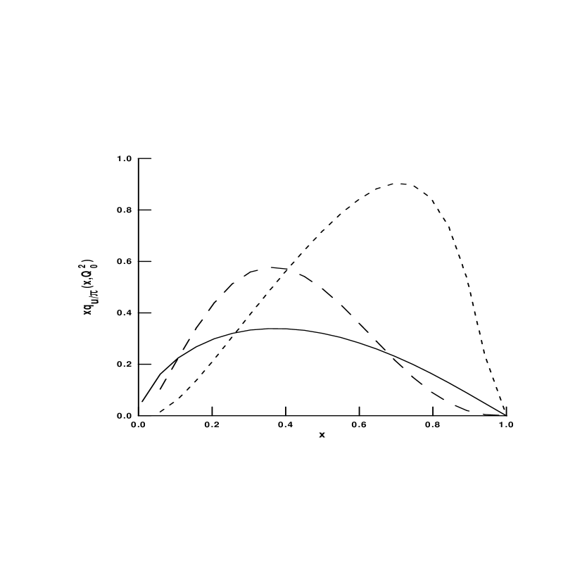
Figure 5: The quark momentum distribution function $xq(x;Q_{0}^{2})$ (long dashed line) for the pion as a function of the variable $x$ evolved to the momentum scale $Q^{2}_{0}=4$ GeV² (LO approximation), using ${\rho}_{c}m_{q}=0.39$ for the density parameter. The solid line denotes the phenomenological curve [3] on the same scale $Q_{0}^{2}$, extracted from the data. The short - dashed line shows the same distribution on the low momentum scale $\mu^{2}_{0}=0.19$ GeV².

In performing the evolution analysis we choose a low momentum scale $\displaystyle\mu_{0}^{2}=0.19\pm 0.05\ GeV^{2}$, and a set for the QCD scale parameter $\Lambda_{QCD}^{(3)}=0.19\ GeV$ in order to be consistent with [3]. The resulting distribution $q(x,Q_{0}^{2})$ is shown in Fig. 5 together with the phenomenological curve derived from the data in [3]. The initial distribution function at the low-momentum scale $\mu_{0}^{2}$ is also shown for comparison.

The values of the first moments of the pion quark distribution at $Q^{2}_{0}=4\ GeV^{2}$ calculated in LO and NLO are shown in Table 2. The error bars quoted in Table 2 for our calculations are due to accepted uncertainty in the choice of the initial scale of evolution $\mu_{0}$. These values should be compared with those obtained from the phenomenological analysis [3] and from LQCD simulations [1]. In Table 2 we also include the moments of quark distribution in the pion obtained from the parametrization [4].

Table 2. The values of the first moments at $Q_{0}^{2}=4$ GeV².

	LO	NLO	LQCD[1]	Exp. fit[3]	Exp. fit[4]
	(this	calculations)
$A_{2}(Q^{2}_{0})$	$0.321\pm 0.02$	$0.293\pm 0.03$	$0.279\pm 0.083$	$0.230\pm 0.01$	$0.193\pm 0.01$
$A_{3}(Q^{2}_{0})$	$0.150\pm 0.02$	$0.112\pm 0.025$	$0.107\pm 0.035$	$0.101\pm 0.005$	$0.083\pm 0.005$
$A_{4}(Q^{2}_{0})$	$0.083\pm 0.015$	$0.057\pm 0.025$	$0.048\pm 0.020$	$0.057\pm 0.005$	$0.046\pm 0.005$

Let us finally discuss the uncertainties of the QCD evolution from the low momentum scale $\mu_{0}$. As we see from Table 2, the difference of the LO and NLO results is in the range of $30\%$. It turns out that the use of a larger initial evolution scale, say $\mu_{0}^{2}\geq 0.3$ GeV², gives a rather good convergence with deviations less than $10\%$, whereas in the opposite case, i.e., for scales smaller than about $0.1$ GeV² the deviations increase and perturbative evolution loses any sense. This behavior has also been observed in analyzes within the NJL model [7].

The comparison shows that our calculations, in particular in NLO, are consistent with the phenomenological analysis of [3] and fairly close to the LQCD results. Both theoretical approaches (LQCD and the instanton model) predict moment values systematically larger than the phenomenological one. One of the reasons for this disagreement may be traced to the quenched approximation which does not take into account any sea-quark contributions at the initial scale, attributing in this way the whole pion momentum to the valence quarks. Indeed, the origin of the $A_{2}$ moment at the initial scale (in the quenched approximation) and its subsequent evolution is purely kinematic and does not depend on the details of the model. In principle, one could match the valence momentum fraction derived in our calculation with that determined in [3] by shifting the initial value $\mu_{0}^{2}$ down to $0.01$ GeV² (see, for instance, [7]a). However, to start a perturbative evolution from this very low scale is formally incorrect and technically amounts to a rather unstable procedure. In our opinion, it is more realistic to expect that including in our analysis contributions from the sea, which may have momentum fractions of an order of $10\%$, the agreement between the theoretical predictions and the phenomenological analysis can be considerably improved. In addition, the effect of nonperturbative evolution [40] from an initial scale $\mu_{0}^{2}$ up to $Q^{2}\sim 1$ GeV² could be important.

7 Results and discussions

In summary, we have presented theoretical predictions for the valence-quark distribution function, eq. (6), and its moments, eq. (42), for the pion. The calculations are based on the instanton model of the QCD vacuum as a candidate treatment of nonperturbative dynamics, expressing the observable hadron properties in terms of fundamental characteristics of the vacuum state. We found that the instanton model describes well the vacuum expectation values of the lowest-dimension quark-gluon operators and the pion low-energy observables. To obtain these results, we have used gauge invariant forms for the dynamically generated quark masses and quark pion vertex. Thus, we are led to express the form of the pion quark distribution function in terms of the effective instanton size $\rho_{c}$, and the quark-mass parameter $m_{q}$. The pion quark distribution function extracted corresponds to a low normalization scale, where the effective instanton approach is justified. It is shown that the validity of parton sum rules for the isospin and total momentum distribution is a consequence of the compositeness condition and the strict implementation of gauge invariance. We have used techniques to derive these results which constitute a complementary approach to lattice simulations and to phenomenological fits to experimental data. Using this distribution function as an input, we obtained the quark distribution function in the pion via standard perturbative evolution to higher momentum values, accessible by experiment. A reasonable agreement with the data was found. In fact, the calculations are performed in the quenched approximation, where the effect of intrinsic quark-gluon sea is neglected. We expect that the effects of the intrinsic quark component of the pion wave function and the nonperturbative evolution at intermediate energy scale provide a better agreement between theoretical predictions and phenomenological analysis.

Acknowledgments

The authors are grateful to I.V. Anikin, M. Birse, D.I. Diakonov, S.B. Gerasimov, P. Kroll, A.E. Maximov, S.V. Mikhailov, M. Polyakov, R. Ruskov, N.G. Stefanis, M.K. Volkov for fruitful discussions of the results. One of us (A.E.D.) thanks the members of the particle physics groups of the Wuppertal University and Instituto de Física Teórica, UNESP, (São Paulo) for their hospitality and interest in the work. This investigation (A.E.D.) was supported in part by the Russian Foundation for Fundamental Research (RFFR) 96-02-18096 and 96-02-18097, St. - Petersburg center for fundamental research grant: 95-0-6.3-20 and by the Heisenberg-Landau program. L.T. also thanks partial support received from Fundação de Amparo à Pesquisa do Estado de São Paulo (FAPESP) and from Conselho Nacional de Desenvolvimento Científico e Tecnológico do Brasil.

Figure 2: Normalized momentum space representation for the same propagators given in Fig.1, corresponding to eqs. (8) (solid line), (14) (long-dashed) and eq.(15) (short-dashed).

Figure 3: Graphical representation of the operator product expansion. The left hand side of this diagram is the imaginary part (Discontinuity) of the forward scattering amplitude. Within OPE it is represented by the convolution of the Wilson coefficient function $C_{NS}(Q^{2})$ of a “hard” parton subprocess (upper block of the right diagram) and the “soft” parton distribution function $q(x,Q^{2})$ (lower block of the right diagram). The constituent quark and pion are depicted by solid and double lines, respectively. The wavy line denotes the virtual photons. $O_{NS}$ is the local operator and cross on the quark line correspond to $\delta(x-(kn))$.

References

- [1] C. Best et al., Phys. Rev. D 56 (1997) 2743.
- [2] G. Martinelli and C.T. Sachrajda, Nucl. Phys. B306 (1988) 865.
- [3] P.J. Sutton, A.D. Martin, R.G. Roberts, and W.J. Stirling, Phys. Rev. D 45 (1992) 2349.
- [4] M. Glück, E. Reya, and A. Vogt, Z. Phys. C, 53 (1992) 651.
-
[5]
NA3 Coll., J. Badier et al., Z. Phys. C 18 (1983) 281;
NA10 Coll., B. Betev et al., Z. Phys. C 28 (1985) 15;
E537 Coll., E. Anassontzis et al., Phys. Rev. D 38 (1988) 1377;
E615 Coll., P. Bordalo et al., Phys. Lett. B 193 (1987) 368;
WA70 Coll., M. Bonesini et al., Z. Phys. C 37 (1988) 535. -
[6]
A.V. Belitsky, Phys. Lett. B 386 (1996) 359;
V.M. Belyaev and M.B. Johnson, Phys. Rev. D 56 (1997) 1481. -
[7]
R. M. Davidson and E. Ruiz Arriola, Phys. Lett.
B 348 (1995) 163;
K. Suzuki, Phys. Lett. B 368 (1996) 1. -
[8]
T. Hatsuda, T. Kunihiro, Phys. Rep. 247 (1994) 221;
D. Ebert, H. Reinhardt, and M.K. Volkov, Progr. Part. Nucl. Phys. 35 (1994) 1. - [9] D. Diakonov, Chiral Symmetry Breaking by Instantons, in Varenna 1995 Selected Topics in Nonperturbative QCD, 397-432, Varenna, Italy (1995); hep/ph-9602375 and references therein.
- [10] T. Schäfer and E.V. Shuryak, Rev. of Mod. Phys. 70(2) (1998) 323, and references therein.
- [11] G. ’t Hooft, Phys. Rev. D 14 (1976) 3432.
- [12] R.D. Carlitz and D.B. Creamer, Ann. Phys. (NY) 118 (1979) 429.
- [13] D.I. Dyakonov and V. Yu. Petrov, Nucl. Phys. B245 (1984) 259.
- [14] D.I. Dyakonov and V. Yu. Petrov, Zh. Eksp. Teor. Fiz. 89 (1985) 751 [Sov. Phys. JETP 62 (1985) 431]; Nucl. Phys. B272 (1986) 457.
- [15] S.V. Esaǐbegyan and S.N. Tamaryan, Yad. Fiz. 49 (1989) 815 [Sov. J. Nucl. Phys. 49 (1989) 507].
- [16] V.B. Rosenhaus and M.G. Ryskin, Yad. Fiz. 44 (1986) 1276 [Sov. J. Nucl. Phys. 44 (1986) 829].
- [17] A.E. Dorokhov and N.I. Kochelev, Phys. Lett. B 304 (1993) 167.
- [18] D.I. Dyakonov, V.Yu Petrov, P.V. Pobylitsa, M.V. Polyakov, and C. Weiss, Nucl. Phys. B480 (1996) 341.
- [19] M. Hutter, Gauge Invariant Quark Propagator in the Instanton Background, München preprint LMU-95-03 (1995); hep-ph/9502361.
- [20] A.E. Dorokhov, S.V. Esaibegyan, and S.V. Mikhailov, Phys. Rev. D 56 (1997) 4062.
- [21] J. Terning, Phys. Rev. D 44 (1991) 887.
-
[22]
R.D. Bowler and M.C. Birse,
Nucl. Phys. A582 (1995) 655;
R.S. Plant and M.C. Birse, Nucl. Phys. A628 (1998) 607. - [23] B. Jouvet, Nouvo Cim. 5 (1957) 1; M.T. Vaughn, R. Aaron, and R.D. Amado, Phys. Rev. 124 (1961) 1258; A. Salam, Nouvo Cim. 25 (1962) 224; S. Weinberg, Phys. Rev. 130 (1963) 776.
-
[24]
E.V. Shuryak, Nucl. Phys. B203 (1982) 93, 116;
E.V. Shuryak, Nucl. Phys. B328 (1989) 102. - [25] See f.i. for a review: A.E. Dorokhov, N.I. Kochelev, and Yu.A. Zubov, Fiz. Elem. Chastits At. Yadra 23 (1992) 1192 [Sov. J.Part. Nucl. Phys. 23 (1992) 522].
-
[26]
H. Kleinert, Phys. Lett. 62B (1976) 429;
T. Kugo, Phys. Lett. 76B (1978) 625;
M.K. Volkov, Ann. Phys. (NY) 157 (1984) 282; Fiz. Elem. Chastits At. Yadra 17 (1986) 433 [Sov. J. Part. Nucl. Phys. 17 (1986) 186]. - [27] S.V. Mikhailov and A.V. Radyushkin, Yad. Fiz. 49 (1989) 794 [Sov. J. Nucl. Phys. 49 (1989) 494]; Phys. Rev. D 45 (1992) 1754.
- [28] M.A. Shifman, A.I. Vainshtein. and V.I. Zakharov, Nucl.Phys B147 (1979) 385, 448.
-
[29]
V. M. Belyaev and B.L.Ioffe,
Zh. Eksp. Teor. Fiz. 83 (1992) 876
[Sov. Phys. JETP 56 (1982) 493];
A. A. Ovchinnikov and A. A. Pivovarov, Yad. Fiz. 48 (1988) 1135 [Sov. J. Nucl. Phys. 48 (1988) 721]. - [30] M.Kremer and G. Schierholz, Phys. Lett. B 194 (1987) 283.
- [31] M.A. Shifman, A.I. Vainshtein and V.I. Zakharov, Nucl. Phys. B163 (1980) 46.
- [32] M.V. Polyakov and C. Weiss, Phys. Lett. B 387 (1996) 841.
-
[33]
D.J. Broadhurst et al., Phys. Lett. B 329 (1994) 103;
B.V. Geshkenbein, Phys. Atom. Nucl. 58 (1995) 1171;
S. Narison, Phys. Lett. B387 (1996) 162. - [34] M. D’Elia, A. Di Giacomo, and E. Meggiolaro, Phys. Lett. B 408 (1997) 315.
- [35] H. Ito, W.W. Buck, and F. Gross, Phys. Rev. C 43 (1992) 2483.
- [36] I. Anikin, M. Ivanov, N. Kulimanova, and V. Lyubovitskii, Phys. Atom. Nucl. 57 (1994) 1082.
- [37] L. Baulieu, E.G. Floratos, and C. Kounnas, Nucl. Phys. B166 (1980) 321.
- [38] S.V. Mikhailov and A.V. Radyushkin, Nucl. Phys. B254 (1985) 89.
- [39] See, e.g., F.J. Ynduráin, Quantum Chromodynamics, Springer Verlag, Berlin, 1983.
- [40] M. Genovese, Nuovo Cim. A 109 (1996) 177.