EUROPEAN LABORATORY FOR PARTICLE PHYSICS

CERN-EP/98-043

March 11th, 1998

The Cambridge jet algorithm:
features and applications

Stan Bentvelsen and Irmtraud Meyer

Jet clustering algorithms are widely used to analyse hadronic events in high energy collisions. Recently a new clustering method, known as ‘Cambridge’, has been introduced. In this article we present an algorithm to determine the transition values of $y_{\mathrm{cut}}$ for this clustering scheme, which allows to resolve any event to a definite number of jets in the final state. We discuss some particularities of the Cambridge clustering method and compare its performance to the Durham clustering scheme for Monte Carlo generated $\mathrm{e^{+}e^{-}}$ annihilation events.

Submitted to Eur. Phys. J. C

1 Introduction

In collider physics, clustering of the experimentally accessible hadronic final states is used to determine the underlying parton structure of events. In $\mathrm{e^{+}e^{-}}$ annihilation the widely known JADE [1] and Durham [2] jet algorithms have become indispensable in this process, permitting a wide range of important tests of QCD, allowing refined measurements of electro-weak physics with hadronic final states and being used in searches for new physics.

Recently a new jet clustering scheme, known as Cambridge, has been introduced [3]. This scheme is a modification of the original Durham $k_{T}$-clustering scheme. The Cambridge algorithm is designed to minimise the formation of spurious ‘junk-jets’, jets formed from a multitude of low transverse momentum particles, unrelated to the underlying parton structure.

For all the above mentioned algorithms, clustering of the final state is performed iteratively and is terminated at a clustering specific resolution scale, generically denoted by the resolution parameter $y_{\mathrm{cut}}$. By changing the value of $y_{\mathrm{cut}}$, the final state is resolved into a varying number of jets. The Cambridge algorithm involves three basic components in this iterative process. It uses an ordering variable, $v_{ij}$, a test variable, $y_{ij}$, and a recombination procedure. In JADE-type jet clustering algorithms only two basic components are involved, since the ordering variable, $v_{ij}$, and the test variable, $y_{ij}$, are identical.

In this note we review the Cambridge finder and discuss some of its experimental peculiarities. In terms of computing this algorithm is more complex compared to the JADE and Durham algorithms. Due to the distinction between test and ordering variables, the sequence of clustering now depends on the value of $y_{\mathrm{cut}}$. We show that the jet multiplicity obtained with this algorithm is not monotonically decreasing for increasing $y_{\mathrm{cut}}$, and that for some events it is impossible to resolve a certain jet multiplicity. Therefore the concept of the ‘transition values in $y_{\mathrm{cut}}$’ has to be defined more precisely. The transition value at which the event classification changes from $n$-jets to $m$-jets, when going to larger values for $y_{\mathrm{cut}}$, will subsequently be referred to as $y^{\mathrm{m\leftarrow n}}$ value.

Next we developed a fast algorithm to obtain the transition values $y^{\mathrm{m\leftarrow n}}$ for the Cambridge finder. Using this algorithm, we compare results for Monte Carlo generated $\mathrm{e^{+}e^{-}}\rightarrow q\bar{q}$ events between the Durham and Cambridge finder. We compare their performance in determining the size of the hadronization corrections. As another example, we determine the performance for hadronic decays of $W^{+}W^{-}$ production at LEP2 [4]. Finally we give our conclusions and cite an address to download our FORTRAN code.

2 The Cambridge algorithm

In JADE-type jet clustering algorithms one iteratively combines particles to form final state jets. First one introduces a ‘test variable’ $y_{ij}$. The pair of two objects $i$ and $j$ with smallest value for $y_{ij}$ is selected and its objects are combined or the iteration is terminated when $y_{ij}>y_{\mathrm{cut}}$ for all pairs of objects. For the JADE and Durham algorithms, the test variables $y_{ij}^{J}$ and $y_{ij}^{D}$ are defined respectively as

$$y_{ij}^{J} = \frac{2E_{i}E_{j}}{E_{vis}^{2}}(1-\cos\theta_{ij})$$ (1)

$$y_{ij}^{D} = \frac{2\min(E_{i}^{2},E_{j}^{2})}{E_{vis}^{2}}(1-\cos\theta_{ij})$$ (2)

where $E_{i}$ and $E_{j}$ denote the energies of particles $i$ and $j$ and $\theta_{ij}$ their opening angle. Note that we normalise the values of $y_{ij}^{J}$ and $y_{ij}^{D}$ to the visible energy, $E_{vis}$, which is the sum of energies for all particles observed in the final state. The second ingredient is the recombination procedure. Normally the $E$-scheme is taken, for which the four-momentum of the resulting object is simply the sum of the four-momenta of the two objects $p_{i}$ and $p_{j}$.

In contrast to this the Cambridge algorithm involves three basic components to form the final state jets. The algorithm starts from a table of $N_{\mathrm{obj}}$ primary objects, which is the set of the particles’ four-momenta. It starts clustering the pair of particles with the smallest opening angle, using the ordering variable $v_{ij}$. The test variable $y_{ij}^{D}$, which is identical to the one for the Durham algorithm, decides when the iterative procedure is stopped. It is subsequently denoted by $y_{ij}$. The algorithm proceeds as follows:

1. If only one object remains, store this as a jet and stop.

2. Select the pair of objects $i$ and $j$ that have the minimal value for their ordering variable, $v_{ij}$, with $v_{ij}=2(1-\cos\theta_{ij})$.

3. Inspect the test variable $y_{ij}$.

   • If $y_{ij}<y_{\mathrm{cut}}$ then combine $i$ and $j$ in a new object using the $E$-scheme. Remove particles $i$ and $j$ from the table of objects that remain to be combined and add the new object with four-momentum $p_{i}+p_{j}$.

   • If $y_{ij}\geq y_{\mathrm{cut}}$ then store the object $i$ or $j$ with the smaller energy as a separated jet and remove it from the table. The higher energetic object remains in the table.

Removing the softer of two resolved objects, as described in the last step, is called soft freezing. It prevents the softer jet from attracting any extra particles, thereby reducing non-intuitive clustering effects.

3 The Cambridge algorithm: an example

In order to test the various clustering algorithms, we generate Monte Carlo $e^{+}e^{-}\rightarrow q\bar{q}$ events at $\sqrt{s}=91.2$ GeV with the PYTHIA event generator [5]. The generation includes parton showering (‘parton-level’), and subsequent fragmentation and decays of the final state (‘hadron-level’). The parameters of the Monte Carlo event generator are adjusted in order to provide an optimal description of large samples of hadronic $Z^{0}$ decay data [6].

Figure 1: Display, projected onto the $xy$-plane, of a $q\bar{q}$ generated event at $\sqrt{s}=91.2$ GeV. The lengths of the arrows are proportional to the energies of the objects. The jet-axes are indicated by the arrows, left at the parton level, right at the hadron level. The particle and jet three-momenta are shown for the Cambridge and Durham algorithms separately. Particle association to jets is indicated with various line-styles. The length of the parton and jet axes are scaled down by a factor of four.

To illustrate the differences between the Cambridge and Durham finders we present in Figure 1 the three-momenta of a typical event projected onto the $xy$-plane. The underlying parton level is shown in the figure by the thick arrows and consists of a quark $q$ recoiling against a $\bar{q}g$ system, with the gluon being relatively soft.

At the hadron level, the event is clustered again to three final state jets, both with the Durham and Cambridge algorithm. The final jets are indicated by thick arrows, and the association of particles to the three jets is indicated by various line styles.

In this example one clearly observes the positive effect of soft freezing on the hadronization corrections. In the Cambridge algorithm the soft gluon jet is separated and classified as a final state jet. Most particles in the hemisphere are assigned in an intuitive way to the quark jet. The three final jets closely resemble the underlying parton structure. In contrast to this, in the Durham algorithm more particles are clustered around the soft gluon, so that the gluon jet becomes even more energetic than the quark jet. It is obvious that in this example the final state found for the Cambridge algorithm resembles the parton structure more than the Durham algorithm.

Figure 2: Example of the jet multiplicity, $N_{\mathrm{jet}}$  as function of $y_{\mathrm{cut}}$ for two Monte Carlo generated events. The dash-dotted line is for the Durham algorithm, the full line for the Cambridge algorithm. The points mark the $y^{\mathrm{m\leftarrow n}}$ transition values.

As an illustration of some of the peculiarities of the Cambridge algorithm, in Figure 2 we present the jet multiplicity as function of $y_{\mathrm{cut}}$ for two events. In the figures the dashed lines correspond to the Durham algorithm, whereas the full lines correspond to the Cambridge clustering. For the Durham algorithm, the jet multiplicity is decreasing monotonically for increasing $y_{\mathrm{cut}}$. In addition, each event can be resolved into each jet-multiplicity $N_{\mathrm{jet}}$, with $1\leq N_{\mathrm{jet}}\leq N_{\mathrm{obj}}$.

In the Cambridge finder the situation is a little more complex, as can be seen in the same figure. In the left plot of Figure 2 an example is given where

• the jet multiplicity is not monotonically decreasing for increasing $y_{\mathrm{cut}}$.

In this example, at the resolution $y_{\mathrm{cut}}\sim 10^{-4.3}$, the jet-multiplicity decreases from 6 to 5 to 4 when $y_{\mathrm{cut}}$ increases, but then increases from 4 to 5 again. At $y_{\mathrm{cut}}\sim 10^{-4.1}$ the multiplicity decreases from 5 to 4. At $y_{\mathrm{cut}}\sim 10^{-3.8}$ a situation occurs where the jet multiplicity does not change from being 4, but the four final state jets change their four-momenta. The jet configuration of the two 5-jet states and three 4-jet state are all different.

In the right plot of Figure 2 we show an example where

• it may not be possible to resolve the event into a certain $n$-jet final state.

In this example, at $y_{\mathrm{cut}}\sim 10^{-3.3}$, the event changes from being classified as a 6 jet event to a 3 jet event. For this event, it is impossible to choose a value for $y_{\mathrm{cut}}$ such that the event is resolved into a 4 or a 5 jet configuration.

As a last ‘peculiarity’ of the Cambridge jet clustering we consider the particle to jet association. For the JADE and Durham algorithms, when crossing a transition value in $y_{\mathrm{cut}}$ towards higher values, two of the jets are merged into one new jet while all other jets are left untouched. The resulting new jet consists of exactly all particles that belonged to the two merged jets, and the subjet history of jets can be traced unambiguously. In the Cambridge algorithm this need not be the case, since the sequence of recombination may be different for different values of $y_{\mathrm{cut}}$. It thus can happen that the particle contents of a jet at a given value for $y_{\mathrm{cut}}$ does not match the sum of the particle contents of two resolved jets at lower values of $y_{\mathrm{cut}}$.

For many applications it is essential to obtain the transition values $y^{\mathrm{m\leftarrow n}}$. For example, in previous studies of $\mathrm{e^{+}e^{-}}$ annihilation data the value of $y^{2\leftarrow 3}$ was analysed in order to obtain $\alpha_{s}(Q^{2})$ [7]. In other studies all events were classified as four [8] or five [9] jets and their angular correlations were studied in order to probe the non-Abelian nature of QCD. In current studies at $\mathrm{e^{+}e^{-}}$ annihilation energies reached by the LEP2 programme [4], events also have to be clustered to four jets in order to determine the $W$-boson characteristics in the hadronic decays of $W^{+}W^{-}$ pairs. Therefore, an algorithm to obtain all transition values $y^{\mathrm{m\leftarrow n}}$ with full information on the particle to jet association is highly desirable.

4 Transition values of ${\bf y_{\mathrm{{\bf cut}}}}$

In the JADE and Durham algorithm, the sequence of clustering of an event can be determined once and completely, and is independent of the value of $y_{\mathrm{cut}}$. From this clustering information about jet multiplicities, four-momenta and jet-particle association, can subsequently be retrieved for any value of $y_{\mathrm{cut}}$. This is the strategy used in the KTCLUS[10] and YKERN [11] packages. The final jet configuration is identical for all values of $y_{\mathrm{cut}}$ between two subsequent transition values. At the transition value $y^{n\leftarrow n+1}$, the event flips from a $n+1$-jet to a $n$-jet configuration. The transition values for the JADE and Durham algorithms are ordered in $y_{\mathrm{cut}}$. Using the transition values one can select a value for $y_{\mathrm{cut}}$ such that the event is resolved into the required number of jets.

In contrast to this, the clustering sequence in the Cambridge algorithm depends on the value of $y_{\mathrm{cut}}$ because it distinguishes between ordering and testing variables. It is therefore no longer straightforward to calculate the transition values. In general, at the transition values $y^{m\leftarrow n}$ the event can flip between a $n$-jet configuration to a $m$-jet configuration where $n$ and $m$ are not necessarily consecutive. As it is important to obtain the values for $y^{\mathrm{m\leftarrow n}}$, it was suggested in [3] to perform a binary search in $y_{\mathrm{cut}}$ to determine these transition values, by repeated evaluation of the clustering. This proposal is not completely satisfactory since such a search has an intrinsic limited precision, might skip over several transition values and becomes very computing time intensive.

We have developed a method to determine the transition values of $y_{\mathrm{cut}}$ for the Cambridge finder exactly, as follows. While performing the clustering at a particular value of $y_{\mathrm{cut}}$, denoted by $y_{\mathrm{init}}$, we keep track of the maximum value of $y_{ij}$, between any two objects $i$ and $j$ encountered in this process, with $y_{ij}$ being always smaller than $y_{\mathrm{init}}$. By construction this maximum value, which we denote by $y^{\mathrm{max}}_{ij}$, is smaller than $y_{\mathrm{init}}$. We now note that for any value of $y_{\mathrm{cut}}\in\left[y^{\mathrm{max}}_{ij},y_{\mathrm{init}}\right)$, the Cambridge algorithm will follow the same clustering sequence. Only when the cluster algorithm is performed with a value $y_{\mathrm{cut}}$ smaller than $y^{\mathrm{max}}_{ij}$, the condition $y_{ij}\geq y_{\mathrm{cut}}$ is satisfied at least once more and the subsequent clustering sequence may change completely. The value $y^{\mathrm{max}}_{ij}$ is therefore one of the $y_{\mathrm{cut}}$ transition values. Note that the clustering may also change completely for values of $y_{\mathrm{cut}}$ larger than $y_{\mathrm{init}}$.

These observations can be utilised to scan the complete region of $y_{\mathrm{cut}}$. We therefore start by clustering the complete event to a one-jet configuration by chosing $y_{\mathrm{cut}}=1$ in the first step. After this step one iteratively repeats the clustering to calculate smaller and smaller values of $y^{\mathrm{max}}_{ij}$ at which the clustering changes, and thereby calculates smaller and smaller transition values. The process terminates if either the number of resolved jets equals the number of input objects or if the desired number of jets is resolved. To summarise:

1. Start with value $y_{\mathrm{init}}=1$ and set $y_{\mathrm{cut}}=y_{\mathrm{init}}$.

2. Perform the Cambridge jet clustering for $N_{\mathrm{obj}}$ objects. During the clustering, keep track of all values of $y_{ij}$ between all objects $i$ and $j$, and determine their maximum value, $y^{\mathrm{max}}_{ij}$.

3. Store the value of $y^{\mathrm{max}}_{ij}$, the number of jets, $n$, their four-momenta and the jet-particle association. The clustering for $y_{\mathrm{cut}}>y^{\mathrm{max}}_{ij}$ is now completely determined.

4. The algorithm stops if:

   • The number of resolved jets equals the number of input objects, $n=N_{\mathrm{obj}}$. Then the event is classified completely and the algorithm necessarily stops.

   • The desired number of jets or a preset lower limit in $y_{\mathrm{cut}}$ is reached, and the algorithm is stopped.

5. Set $y_{\mathrm{cut}}=y^{\mathrm{max}}_{ij}$ and go to step 2.

Once this process has been performed, all information about the clustering is accessible without any appreciable additional computing time. The total amount of computing time is proportional to the desired jet-multiplicity. For example, to study four jet final states with the Cambridge finder requires approximately four times as much computing time compared to the Durham or JADE algorithms.
Instead of the top-down approach for which the clustering starts at $y_{\mathrm{cut}}=1$ as explained above, a bottom-up approach is in principle also possible. One may implement the bottom-up approach by starting the clustering at the lowest value $y_{\mathrm{cut}}=0$. For $N_{\mathrm{obj}}$ given at the start of the clustering, one finds the pair of objects with smallest value $v_{ij}$ (corresponding to the pair closest in angle) and determines the corresponding value for $y_{ij}$. Then the two possible cases are considered: one in which the softer object is frozen, the other in which the two objects are combined. In both cases the number of objects that remain to be combined is reduced by one. This combinatorical procedure is subsequently continued, and all possible clustering sequences are listed. The procedure terminates when only one object remains.

From the corresponding values for $y_{ij}$, saved for each step, one can deduce the final transition values $y^{\mathrm{m\leftarrow n}}$ and the jet configuration associated to them. Note that the number of possible clustering sequences is proportional to $2^{N_{\mathrm{obj}}+1}$, which limits the practical use of the bottom-up approach.

5 Monte Carlo results

Jet finder comparison and hadronization corrections

With the transition values $y^{\mathrm{m\leftarrow n}}$ defined both for the Cambridge and Durham algorithms, we compare, as an example, the values for $y^{2\leftarrow 3}$. In [12] similar studies have been performed to compare the performance of the Durham and JADE algorithms. In all the following we will define the region with the highest value for $y_{\mathrm{cut}}$ as the nominal $y_{\mathrm{cut}}$ region. Here, in Figure 3a we show the correlation of the Cambridge and Durham algorithms for $y^{2\leftarrow 3}$ at the parton level, at the end of the PYTHIA parton shower. For most of our generated events, the obtained values for $y^{2\leftarrow 3}$ are identical for the Cambridge and the Durham algorithms (approximately 75% of the events are found on the line in the figure). For a small fraction of events, the value obtained with the Cambridge algorithm is smaller compared to the value for the Durham algorithm. At the hadron level, as shown in Figure 3b, the values at low $y^{2\leftarrow 3}$ obtained using the Cambridge algorithm are smaller for almost all events, but become similar for the two algorithms for increasing values of $y^{2\leftarrow 3}$. At the hadron level, approximately 15% of the events have identical values for $y^{2\leftarrow 3}$ for both algorithms.

Next, in Figure 4a and 4b, we compare the hadronization corrections for the Cambridge and Durham algorithms. We present the correlation between the transition values $y^{2\leftarrow 3}$ calculated at the hadron and at the parton level, for both. The line indicates the ideal case for which equal values for $y^{2\leftarrow 3}$ at both levels are found. For the Durham algorithm the difference in $y^{2\leftarrow 3}$ at the parton and hadron level is small. When going to lower $y^{2\leftarrow 3}$ values, the distribution broadens and shifts toward smaller $y^{2\leftarrow 3}$ values at the hadron level. For the Cambridge algorithm, at high values of $y^{2\leftarrow 3}$ the parton and hadron level correlation is similar to the one for the Durham algorithm. Whereas, when going to smaller values for $y^{2\leftarrow 3}$, the values at the hadron level get increasingly larger with respect to the parton level values. The width of the distribution is similar to that for the Durham algorithm. In order to quantify the differences, we calculated the mean of the logarithmic ratio of the $y^{2\leftarrow 3}$ values for the parton level and the hadron level: this value equals $0.232\pm 0.002$ for the Durham algorithm, and $0.257\pm 0.002$ for the Cambridge algorithm, which indicates that the overall hadronization corrections for the Durham algorithm are $\sim 10$% smaller than for the Cambridge algorithm. Note however that the hadronization corrections do not only depend on the jet algorithm but also on the hadronization model used.

Figure 3: Monte Carlo generated events at $\sqrt{s}=91.2$ GeV using PYTHIA [5]. In a) we present the correlation between $y^{2\leftarrow 3}$ calculated using the Cambridge and $y^{2\leftarrow 3}$ calculated using the Durham algorithm, at the parton level. Note that the majority of events have identical values of $y^{2\leftarrow 3}$ for both algorithms. In b) the same is shown for the hadron level.

Figure 4: Monte Carlo generated events at $\sqrt{s}=91.2$ GeV using PYTHIA [5]. In a) we present the correlation between $y^{2\leftarrow 3}$ calculated at the parton level and $y^{2\leftarrow 3}$ calculated at the hadron level, using the Durham algorithm. In b) the same is shown for the Cambridge algorithm.

The mean hadronization corrections can be studied more directly, as a function of $y_{\mathrm{cut}}$, from plots as presented in Figures 5a and 5b. In Figure 5a we show the mean of the logarithmic ratio of the values $y^{2\leftarrow 3}$ for the parton and hadron level, $\left<\log_{10}(y^{2\leftarrow 3}_{parton}/y^{2\leftarrow 3}_{hadron})\right>$, as a function of the transition value at the parton level. When calculating the mean deviation between hadron and parton level for each value $y^{2\leftarrow 3}$, the contribution to the hadronization corrections for many events may cancel. To exclude effects due to cancellation we present in Figure 5b the size of the hadronization corrections. We show the mean absolute difference of $y^{2\leftarrow 3}$ calculated on the parton and at the hadron level, $\left<\mbox{Abs}\left(\log_{10}(y^{2\leftarrow 3}_{parton}/y^{2\leftarrow 3}_{hadron})\right)\right>$, as a function of $y^{2\leftarrow 3}$ calculated at the parton level.

Figure 5: In a) we show for both the Cambridge and the Durham algorithms the mean logarithmic ratio between $y^{2\leftarrow 3}$ calculated at the parton and the hadron level, as function of $y^{2\leftarrow 3}$ at the parton level, using the PYTHIA event generator. Identical values for $y^{2\leftarrow 3}$ are represented by the full horizontal line. The dashed lines correspond to a deviation between the parton and hadron level by a factor of two. In b) we present the absolute value of the mean as calculated in a). The three regions indicated in both figures by $I$, $II$ and $III$ are discussed in the text.

Figure 6: In a) we present the relative jet production rates $R_{n}$, as a function of $y_{\mathrm{cut}}$, for the Durham algorithm, using the PYTHIA event generator. The full lines with the points correspond to the hadron level and the dashed line correspond to the parton level. For $R_{5}$ we summed all contributions for jet multiplicities of 5 and larger. In b) the same is shown for the Cambridge algorithm.

To compare the performance of the two jet finders we distinguish in Figure 5a and 5b three regions in $y^{2\leftarrow 3}$, denoted by $I$, $II$ and $III$. In region $I$, for values of $y^{2\leftarrow 3}$ above $10^{-2}$, the hadronization corrections are small and comparable for both algorithms. A fraction of about 37% of our generated events belongs to this region.

Region $II$ is defined for values of $y^{2\leftarrow 3}$ between $10^{-3.2}$ and $10^{-2}$. In this region differences between the two algorithms occur. The mean deviation for the Durham algorithm reaches a maximum of about 20%, and vanishes at $y^{2\leftarrow 3}\sim 10^{-2.8}$, as can be seen in Figure 5a. However, Figure 5b shows that this decrease is due to cancellations and that the absolute hadronization corrections increase at $y^{2\leftarrow 3}\sim 10^{-2.8}$. For the Cambridge algorithm a different behaviour is observed. The mean deviation reaches a maximum of 100% for this algorithm, at $y^{2\leftarrow 3}\sim 10^{-2.6}$, implying large hadronization corrections. The absolute hadronization corrections for the Cambridge algorithm, as shown in Figure 5b, reach a maximum at about $10^{-2.6}$, and then decrease until the value for the Durham algorithm is reached. In the whole region $II$, where about 49% of our generated events can be found, hadronization corrections for the Cambridge algorithm are significantly larger than for the Durham algorithm.

In region $III$, for values of $y^{2\leftarrow 3}$ below $10^{-3.2}$, the figures show that the hadronization corrections are large for both algorithms and that they increase rapidly towards smaller values of $y^{2\leftarrow 3}$. The corrections for the Cambridge algorithm are smaller compared to the Durham algorithm. However, only about 14% of our generated events can be found in region $III$.

Our analysis of the hadronization corrections for $y^{2\leftarrow 3}$ shows that the Cambridge algorithm performs clearly better only in the region of low $y^{2\leftarrow 3}$ values (region $III$). This region contains 14% of the events and the corrections there are large for both algorithms. In all other regions the Durham finder performs equally well (region $I$) or even significantly better (region $II$). These two regions contain a fraction of 85% of our generated $\mathrm{e^{+}e^{-}}\rightarrow q\bar{q}$ events. These basic tendencies of the hadronization corrections are also found when studying the transition value $y^{3\leftarrow 4}$. Note that for very low values of $y_{\mathrm{cut}}$ the approximations used for the implemention of QCD in PYTHIA might not give a reliable description of the hadronization process. Therefore, for very low values of $y_{\mathrm{cut}}$ the jets returned by the Cambridge algorithm may correspond closer to the underlying parton structure than can be shown in these Monte Carlo studies.
Classical tests of QCD rely on relative production rates for multijet hadronic decays, defined as $R_{n}=\sigma_{n}/\sigma_{tot}$ [11]. In Figures 6a and 6b we present the relative production rates for two, three, four, and five or more jet final states, for the hadron level and the parton level. For these figures we used the same set of $\mathrm{e^{+}e^{-}}\rightarrow q\bar{q}$ events as before. In Figure 6a the performance for the Durham algorithm is shown. For all $y_{\mathrm{cut}}$ values between one and approximately $10^{-2.8}$ the hadron and parton level agree reasonably well. When going to smaller values of $y_{\mathrm{cut}}$ the curves for the two levels increasingly deviate. For the Cambridge algorithm the hadronization corrections are larger for the region in $y_{\mathrm{cut}}$ where the Durham algorithm performs well, between $y_{\mathrm{cut}}$ of one and approximately $10^{-2.8}$. However, when going to lower values of $y_{\mathrm{cut}}$  the differences between hadron and parton level are, for most jet multiplicities, smaller than for the Durham algorithm.

To summarise our investigations of the hadronization corrections, we conclude that the Durham algorithm provides smaller hadronization corrections for a large region in $y_{\mathrm{cut}}$.

In [3], the hadronization corrections for the mean jet multiplicity, $\left<n_{jet}\right>=\sum_{1}^{\infty}nR_{n}$, was studied. There it was found that hadronization corrections for the Cambridge and Durham algorithms are small for values of $y_{\mathrm{cut}}>10^{-3.2}$. Our Figures 6b show that for these values of $y_{\mathrm{cut}}$ the hadronization corrections for each jet production rate, $R_{n}$, are sizable for the Cambridge algorithm, whereas for the Durham algorithm they are small. The small hadronization corrections found for the Cambridge algorithm in the study of the mean jet rate $\left<n_{jet}\right>$ are due to fortuitous cancellations in the individual jet production rates.

Multiple and impossible jet multiplicities

As already indicated, the transition values $y^{\mathrm{m\leftarrow n}}$ in the Cambridge algorithm need not be the transition between two consecutive jet-multiplicities. Several intervals in $y_{\mathrm{cut}}$ may lead to the same jet-multiplicity, and they have in general different jet four-momenta. Secondly, it need not always be possible to cluster the event to any required jet multiplicity.

Figure 7: The full points show, as a function of $n$-jet, the fraction of events for which multiple $n$-jet final states could be reconstructed. This is done for a set of $\mathrm{e^{+}e^{-}}\rightarrow q\bar{q}$ generated events. The open points show, as a function of $n$-jet, the fraction of events for which no $n$-jet final state could be reconstructed. All points are normalised to the overall number of generated events.

In order to determine the frequency that this might occur, we generated for Figure 7 $e^{+}e^{-}\rightarrow q\bar{q}$ Monte Carlo events with full hadronization, at $\sqrt{s}=91.2$ GeV. The full points present the fraction of events that have multiple regions in $y_{\mathrm{cut}}$ with the same jet multiplicity, as a function of the jet-multiplicity. For our generated events, for example, about 2.2% have multiple regions in $y_{\mathrm{cut}}$ that lead to a four-jet final state, albeit with different jet four-momenta. In the same figure the open points show the fraction of events were the indicated number of jets could not be resolved. For example, in about 2.5% of events no four-jet configuration could be found.

The figure shows that the fraction of impossible jet multiplicities and multiple jet multiplicities increases with increasing $n$, reaches a maximum at around $n=12$, and decreases again. The generated events have a mean total multiplicity of 44.2, and 95% of the events have a multiplicity larger than 25. Note that both distributions are naturally limited by the input number of four-momenta in each event.

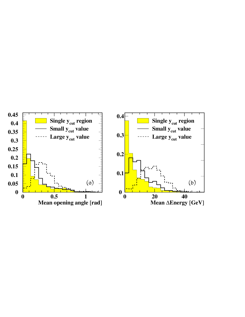
Figure 8: Monte Carlo generated $W^{+}W^{-}$ events at $\sqrt{s}=184$ GeV. In a) we present the mean of the opening angles between the momenta of the four partons and of the four jets at the hadron level. The shaded histogram shows the events for which one four-jet configuration was found. The open histograms correspond to the set of events were the Cambridge algorithm returned two four-jet configurations. The one with the dashed line corresponds to the configuration with the higher values of $y_{\mathrm{cut}}$, whereas the one with the full line corresponds to the configuration with the lower values of $y_{\mathrm{cut}}$. In b) the same is shown, but for the mean absolute energy difference between the four parton and hadron jets.

As another example we generated hadronic decays of $W^{+}W^{-}$ pairs at LEP2 [4] using PYTHIA: $\mathrm{e^{+}e^{-}}\rightarrow W^{+}W^{-}\rightarrow q\bar{q}^{\prime}q^{\prime\prime}\bar{q}^{\prime\prime\prime}$, at $\sqrt{s}=184$ GeV. Information about the kinematics of the two $W$’s can be obtained by forcing the hadronic final state to four jets.

Using the Cambridge finder, we find that about 0.9% of the events have multiple regions in $y_{\mathrm{cut}}$ with four final state jets. For those events one therefore has the freedom to select the set of jets with the larger $y_{\mathrm{cut}}$ values, or the set with the smaller $y_{\mathrm{cut}}$ values. Clearly the selection which corresponds closer to the four primary partons is preferred. In Figure 8a we compare the mean opening angle between the jets and primary four partons, and in Figure 8b the mean absolute energy difference between the jets and the primary partons. It can be clearly seen that in both cases the resolution is better for the fraction of 99% of events in which only one four-jet configuration is found. For the small fraction of events where two four-jet configurations were found, the jet configuration with the lower values of $y_{\mathrm{cut}}$ matches the four primary partons better than the one with larger values of $y_{\mathrm{cut}}$, which can be explained by the following observation. In the majority of events for which the Cambridge algorithm returned two four jet configurations the appearance of hard gluon radiation in the parton shower was observed. Detailed inspection revealed that the hard gluon, radiated from a quark-pair originating from one $W$, points in the direction of a quark originating from the other $W$. The configuration with the low value of $y_{\mathrm{cut}}$ correctly separates the gluon from this quark by the mechanism of soft-freezing, whereas they are merged for the configuration with the larger value of $y_{\mathrm{cut}}$. The correspondence between partons and jets is therefore better in the configuration with the lower value of $y_{\mathrm{cut}}$.

6 Conclusions

In this note we review the Cambridge jet clustering algorithm, as was recently introduced in [3]. We show some of its particularities for Monte Carlo generated events. Firstly, the algorithm may find several regions in $y_{\mathrm{cut}}$ with identical final state multiplicity, but different jet four-momenta. Secondly, for some events it is impossible to resolve a certain jet multiplicity. Both these properties are absent in the JADE and Durham algorithms.

We propose a fast, new algorithm that is able to determine the transition values for $y_{\mathrm{cut}}$, based on the YCLUS package. All transition values, jet multiplicities, jet four-momenta and the jet to particle associations are derived and stored, and can be subsequently inferred for all values of $y_{\mathrm{cut}}$ without any substantial additional computing time.

Using this algorithm we determine the hadronization corrections of $\mathrm{e^{+}e^{-}}\rightarrow q\bar{q}$ generated events according to PYTHIA, by comparing parton and hadron level values for $y^{2\leftarrow 3}$, both for the Durham and Cambridge algorithms. This comparative study of the two algorithms is completed by a presentation of the relative jet production rates. For a large interval of $y_{\mathrm{cut}}$ values the hadronization corrections for the Cambridge algorithm are found to be significantly larger than for the Durham algorithm. However, in the region of very small values of $y_{\mathrm{cut}}$ ($y_{\mathrm{cut}}<10^{-3.2}$), the hadronization corrections are large, but better under control for the Cambridge algorithm. Note that for very low values of $y_{\mathrm{cut}}$ the reliability of the comparative Monte Carlo studies is limited due to the fact that for these values of $y_{\mathrm{cut}}$ the approximations used for the implementation of QCD in PYTHIA might not give an appropriate description of the hadronization process.

Further, we present for the Cambridge algorithm the fraction of events for which certain jet multiplicity could never be resolved, or could be resolved multiple times. Four jet final states were explicitly studied in hadronic decays of $W^{+}W^{-}$ events. The large fraction of events where just one four jet configuration was found has better energy and angular resolution than the small fraction of events with multiple four jet configurations.

Fortran code, containing our CKERN routines to obtain the $y_{\mathrm{cut}}$ transition values, can be obtained from the World-Wide Web at

http://wwwcn1.cern.ch/~stanb/ckern/ckern.html.

7 Acknowledgements

We would like to thank S. Bethke for help and inspiring discussions, as well as B. Webber, Yu. Dokshitzer, S. Moretti and Z. Trocsanyi for comments. We like to thank CERN for its hospitality and in particular the OPAL collaboration for providing indispensable recourses.

References

- [1] JADE Collaboration, W. Bartel et al., Phys. Lett. B123(1993)460; Z. Phys. C33(1986)23.
- [2] Yu. L. Dokshitzer, Contribution cited in Report of the Hard QCD Working Group, Proc. Workshop on Jet Studies at LEP and HERA, Durham, December 1990, J. Phys. G17(1991)1537.
- [3] Yu. L. Dokshitzer, G. Leder, S. Moretti and B. Webber, JHEP 08(1997)001.
- [4] The OPAL Collaboration, K. Ackerstaff et al. Eur. Phys. J. C1(1998)395.
- [5] PYTHIA 5.722: T. Sjöstrand, Comput. Phys. Commun. 82(1994)74.
- [6] OPAL Collaboration, G. Alexander et al., Z. Phys. C69(1996)543.
-
[7]
OPAL Collaboration, M. Z. Akrawy et al., Phys. Lett. B235(1990)389,
Mark-II Collaboration, S. Komamiya et al., Phys. Rev. Lett., 64(1990)987. -
[8]
DELPHI Collaboration, P. Abreu et al., Phys. Lett. B414(1997)401,
ALEPH Collaboration, D. Decamp et al., Z. Phys. C76(1997)1
OPAL Collaboration, R. Akers et al., Z. Phys. C65(1995)367. - [9] OPAL Collaboration, R. Akers et al., OPAL Internal Physics Note 188(1995)
-
[10]
M. H. Seymour, Z. Physik C62(1994)127:
KTCLUS program available at http://hepwww.rl.ac.uk/theory/seymour/ktclus/ -
[11]
OPAL Collaboration, M. Z. Akrawy et al., Z. Phys. C49(1991)375,
OPAL Collaboration, P. Acton et al., Z. Phys. C55(1992)1. -
[12]
S. Bethke, Z. Kunszt, D.E. Soper and W.J. Stirling,
Nucl. Phys. B370(1992)310.
S. Bethke, Z. Kunszt, D.E. Soper and W.J. Stirling, Erratum: Jet Clustering Algorithms in Annihilation, hep-ph/9803267.