PHASE TRANSITIONS IN THE UNIVERSE

Marcelo Gleiser

Department of Physics and Astronomy

Dartmouth College

Hanover, NH 03755, USA

and

Nasa/Fermilab Astrophysics Center

Fermi National Accelerator Laboratory

Batavia, IL 60510, USA

and

Osservatorio Astronomico di Roma

Vialle del Parco Mellini, 84

Roma I-00136, Italy

ABSTRACT

During the past two decades, cosmologists turned to particle physics in order to explore the physics of the very early Universe. The main link between the physics of the smallest and largest structures in the Universe is the idea of spontaneous symmetry breaking, familiar from condensed matter physics. Implementing this mechanism into cosmology leads to the interesting possibility that phase transitions related to the breaking of symmetries in high energy particle physics took place during the early history of the Universe. These cosmological phase transitions may help us understand many of the challenges faced by the standard hot Big Bang model of cosmology, while offering a unique window into the very early Universe and the physics of high energy particle interactions.

I- The Universe we know

The fascination with grand questions is as old as time. Some of the earliest records we have of ancient cultures, produced long before what we now call science existed, tell stories about the creation of the world or about the Sun, the Moon, and the visible planets. Although many empires have risen and fallen since then, and society has gone through countless transformations, this fascination with grand questions has remained. It seems that we just cannot avoid being curious about our origin, our future or that of the world as a whole [1].

With the development of modern science, physicists and astronomers have continued this ancient tradition of asking grand questions about the world around us. In 1609 Galileo pointed a telescope to the skies for the first time, revealing a cosmos completely different from the then prevalent Aristotelian view, while later in the same century Newton unified the physics of earthly phenomena with that of the skies through his law of universal gravitation.

But it was during the 20th century, through the marriage of Einstein’s new theory of gravity, the general theory of relativity, and the construction of large telescopes, that physicists and astronomers could really begin to face quantitatively questions concerning the origin and future of our world and of our place in it. Hence was born modern cosmology, the branch of physics which studies the properties and evolution of the Universe as a whole.

In 1929, the American astronomer Edwin Hubble made the incredible discovery that the Universe is expanding. Studying the spectra of galaxies, he showed that the spectra were in general shifted towards the red, indicating that these galaxies were moving away from us [2]. Before him, a few theorists showed that some of the solutions obtained when applying Einstein’s equations of general relativity to the Universe as a whole implied that the Universe could be expanding [3].

But what does this really mean, an expanding Universe? First, a few words about general relativity. According to Einstein’s theory, gravity can be understood as a deformation in the geometry of space and in the flow of time due to the presence of matter. In the absence of matter, space is flat and time flows undisturbed. One can think of a marble rolling on a flat tabletop as a two dimensional analogy. When matter is present things change dramatically. Imagine that the tabletop is made of an elastic material. Now place a heavy lead ball in its centre. The table top won’t be flat anymore, due to the presence of the ball. This is a somewhat simplified view of what happens to the geometry of space in the presence of mass. The trajectories of the marbles will deviate from straight lines due to the curvature of space. Thus, Einstein explained the acceleration caused by gravity as being simply motion in curved space.

Now we can go back to the question of the expansion of the Universe. Since the main force controlling the expansion is gravity, the evolution of the Universe will depend on its total mass. If the average density of matter is equal or smaller than a critical value of about $10^{-29}{\rm g/cm}^{3}$, the Universe will continue its expansion forever. Otherwise, the Universe will collapse onto itself, possibly alternating cycles of expansion and contraction. What is important to stress here is that the expansion of the Universe is an expansion of its geometry. Galaxies are moving away from each other because they are being carried by the expanding geometry, somewhat like corks passively floating down a sloping river [4].

In 1946, George Gamow, a Russian physicist working in the United States, inspired by ideas from the Russian meteorologist-turned-cosmologist Alexander Friedmann and from the Belgian physicist (and priest) George Lemaître, proposed that the Universe emerged from a hot and dense soup of particles and that it has been expanding ever since. Applying what was then known of nuclear physics to a mixture of thermodynamics and general relativity, Gamow and his collaborators were able to reconstruct the history of the first few minutes (actually about half an hour with nuclear data from 1950) of the Universe’s infancy, starting from this primordial hot and dense soup of mainly protons, neutrons, electrons, and photons. This model became later known as the hot Big Bang model of cosmology [5].

The mathematical equations that dictate the evolution of the geometry in the Big Bang model are quite simple [4]. Assuming that the Universe is homogeneous (same everywhere) and isotropic (same in all directions), the geometry is characterized by one single function of time, the scale factor $R(t)$ and by one parameter $k$, which determines if the geometry is closed like that of a sphere ($k=1$), flat ($k=0$), or open ($k=-1$) like that of a saddle. Basically, the scale factor measures how the geometry stretches in time. Assuming further that matter can be modelled by an ideal gas with energy density $\rho(t)$ and pressure $p(t)$, Einstein’s equations determine the dynamics of the scale factor $R(t)$ as follows,

$$\left({{\dot{R}}\over R}\right)^{2}\equiv H^{2}={{8\pi G}\over 3}\rho+{k\over{R^{2}}}~{},$$

and

$$2{{\ddot{R}}\over R}+\left({{\dot{R}}\over R}\right)^{2}=-8\pi Gp-{k\over{R^{2}}}~{}.$$

$H(t)$ is the Hubble factor. Note that $H^{-1}$ defines the time scale at which quantities change in an expanding Universe. This time scale corresponds to a length scale called the Hubble radius, $d_{H}(t)=H(t)^{-1}$. Processes can only operate coherently within the Hubble radius.

The equations above are suplemented by the first law of thermodynamics,

$$d\left(\rho R^{3}\right)=-pd\left(R^{3}\right)~{}.$$

These three equations are related by an identity called the Bianchi identity. Thus, we can choose just two as independent equations. The Friedmann models use the first and third equations. For a simple equation of state, $p=\omega\rho$, we can find a relation between the energy density $\rho$ and the scale factor $R(t)$. There are three cases of interest, fixed by the choice of the constant parameter $\omega$:

$${\rm radiation}:\omega={1\over 3}\Rightarrow\rho\propto R^{-4},$$

$${\rm cold~{}matter}:\omega=0\Rightarrow\rho\propto R^{-3},$$

$${\rm vacuum~{}energy}:\omega=-1\Rightarrow\rho={\rm constant}~{}.$$

Each of these cases is characterized by a different time evolution of the scale factor: $R\propto t^{1/2}$ for radiation, $R\propto t^{2/3}$ for cold matter, and $R\propto{\rm exp}(\sqrt{\Lambda_{\rm vac}}t)$ for vacuum energy, where $\Lambda_{\rm vac}=8\pi G\rho/3$. The relevance of this last case will become clear further on. In general, the total energy density is a combination of all three kinds of matter. However, the evolution of the scale factor is determined by the contribution that dominates the energy density. For example, before $t_{\rm EQ}\sim 4\times 10^{10}{\rm sec}$, radiation dominated over cold matter. Here we will be mostly interested in times $t<t_{\rm EQ}$, that is, in a radiation-dominated Universe, the realm of cosmological phase transitions.

What was remarkable about Gamow’s proposal is that it made two crucial predictions about our present Universe, which could be verified by observations. First, that the Universe should be permeated by electromagnetic radiation with wavelength on the microwave region and temperature of a few degrees above absolute zero. These were the remnant photons from the epoch when hydrogen atoms were made, roughly around 300,000 years after the bang (in today’s numbers).

Second, that light nuclei such as deuterium (${\rm H}_{1}^{2}$), tritium ( ${\rm H}_{1}^{3}$), helium 4 (${\rm He}_{2}^{4}$), helium 3 (${\rm He}_{2}^{3}$), and lithium 7 (${\rm Li}_{3}^{7}$) were cooked when the Universe was about 1 second old (in today’s numbers), during an epoch called “nucleosynthesis” and with calculable proportions [6]. Thus, Gamow and his collaborators predicted that about $24\%$ of the Universe is made of ${\rm He}_{2}^{4}$.

During the past three decades, a growing amount of observational evidence has offered very strong support for the Big Bang model. The cosmic background radiation has been found by Penzias and Wilson in 1965, and is currently the object of intense study by several groups in the world [7, 8]. The abundances of light nuclei have been observed to be consistent with the nucleosynthesis predictions with one free paramenter, the relative excess of matter over antimatter, something we will discuss further down. The fact that the Universe was once very hot and dense as described by the Big Bang model is now widely accepted by the vast majority of physicists and astronomers.

II - Challenges to the Big Bang model

But not everything is fireworks. As with any model in physics, the Big Bang model has its limitations. It describes very successfully the evolution of the Universe from a hot and dense initial state, but fails to address several questions which are of great interest to modern cosmology. The application of atomic physics to cosmology led to the understanding of the generation of the microwave background radiation; the application of nuclear physics led to the understanding of the formation of light nuclei during nucleosynthesis. Now, in order to progress further with our understanding of the early Universe, we must apply higher energy physics to cosmology. For the past two decades or so, physicists have explored the possible consequences of applying particle physics, the physics of subnuclear structures, to the Universe’s infancy. The topic of this article lies precisely in this interface between particle physics and cosmology and on how this interface may help resolve some of the challenges faced by the Big Bang model today. Before we move on, here is a sample of questions that keep modern cosmologists busy.

$\bullet$ The smoothness problem: One of the most startling properties of the cosmic background radiation is its incredible smoothness. By smoothness I mean the lack of variarion in the temperature of the photons as measured in all directions of the sky. When radio antennas are pointed at different angles to measure the temperature of the cosmic background, they find it to be $T=2.726\pm 0.005$ Kelvin, with deviations of less than 0.03%. These beautiful measurements present cosmologists with a serious problem. Regions of the sky now separated by more than about a few degrees were not in causal contact when the microwave radiation was produced, as indicated in the figure. That is, due to the finiteness of the speed of light, interactions between particles that could insure thermal contact and homogeneity were not active beyond what today is a small patch in the sky. If this is the case, how come all sky has the same temperature?

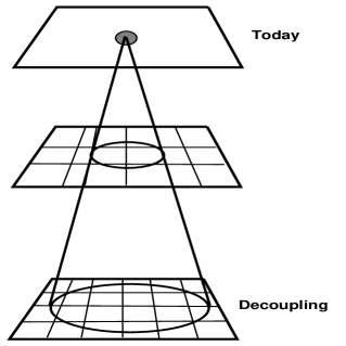
Figure 1: The smoothness problem: A small patch in the sky today corresponds to many causally disconnected regions during decoupling. Yet, the temperature of the cosmic background radiation today is the same over the whole sky.

$\bullet$ The large-scale structure problem: Some astronomers nowadays are doing what great sailors of the 16th century did: extending the frontiers of the world, and mapping the new lands found beyond. Making a map of the visible Universe is an extremely cumbersome task. Basically, one has to identify each galaxy (actually, a statistically representative sample of galaxies) and mark its position in a three dimensional model of the cosmos. Apart from the obvious impossibility of actually locating each galaxy (there are several billions of them out there), one has to be able to measure its position, something which is quite complicated when we are dealing with distances ranging from millions to billions of light years away from us. As a consequence, at this point in time, our maps of the Universe are somewhat approximate, and may look to future generations of astronomers as naive as the maps from the 16th century look to us today.

Still, our maps of the sky reveal something quite unexpected. In principle, we would expect the galaxies to be scattered across the Universe without any sort of pattern, in a perfectly random way. Instead, what is revealed by these maps is a richly-structured Universe, where galaxies tend to lay on vast sheet-like structures surrounding large empty regions, somewhat like the foamy patterns we see in bubble baths [9]. Some of those empty regions, or voids, have diameters of tens of Megaparsecs, or several million light years. ($1{\rm Mpc}=3.26\times 10^{6}{\rm light~{}years}=3.09\times 10^{24}{\rm cm}$). Why would galaxies choose this rather particular distribution, as opposed to being simply scattered across the sky without forming any obvious large-scale patterns?

Figure 2: Voids: A three-dimensional view of voids in the SSRS2 survey. Voids are regions (bubbles here) of space where very few galaxies are found. [Figure can be found in H. El-Ad, T. Piran, and L. N. da Costa, Ap. J. Lett. 462, (1996) L13.]

$\bullet$ The matter-antimatter problem: Most of us learned in high school that matter is made of atoms and that atoms are made of protons, neutrons and electrons. What we don’t usually learn in high school is that to each particle of matter there is another particle, an “anti-particle”, which is essentially the same as the particle but with opposite electric charge. Thus, the electron has its “anti-electron”, called a positron, which has positive electric charge, the proton has an anti-proton, and so on. According to the laws of particle physics, matter and anti-matter should be present in the Universe in equal amounts. And yet, we have ample observational evidence that, at least in a very large volume extending far beyond our galaxy, there is much more matter than anti-matter [10, 11].

When particles collide with their anti-particles, the effects are devastating; they both disintegrate into electromagnetic radiation, their energy carried away in photons. In other words, if there were as much matter as anti-matter in the Universe, we wouldn’t be here asking grand questions. The Universe is somehow unbalanced, biased toward the existence of matter over anti-matter. One of the greatest challenges in modern cosmology is to unveil the roots of this cosmic imperfection.

Now that we have a sample of open challenges to cosmology, we can examine how particle physics can help clarify them. As we will see, the application of particle physics to early Universe cosmology will in many cases invoke another branch of physics, perhaps more familiar to everyday life than the physics of the very large or the very small; the physics of phase transitions.

III-Particles, Forces, and Symmetry Breaking

Matter is organized in a hierarchical structure. Molecules are made of atoms, and atoms of electrons orbiting nuclei made of protons and neutrons. Protons and neutrons are examples of hundreds of particles found in particle accelerators called hadrons, which (fortunately!) are not elementary, but made of yet smaller constituents called quarks. So far, six quarks have been found. The distinctive feature of hadrons is that they interact via the strong nuclear force, the force responsible for keeping the atomic nucleus together. They come in two types, baryons like the proton and the neutron, which are made of three quarks, and mesons, which are made of a quark and an anti-quark. For example, a proton is made of two up quarks and one down quark, while a neutron is made of an up quark and two down quarks.

According to modern particle physics, matter is made of two types of elementary particles, quarks and leptons. The electron is a lepton, and so is the muon. More recently another lepton has been found, the tau, which is heavier than a proton. The name lepton, which comes from the Greek for light weight, is a bit of an anachronism. Each of the three leptons comes with its own neutrino, a massless and neutral particle. The three neutrinos bring the number of leptons to six.

The distinctive feature of the leptons is that they interact via the other force active at subnuclear distances, the weak force. In several situations (but not all) when a lepton interacts via the weak force, its associated neutrino appears. The best-known example is beta decay, where a free neutron decays into a proton, an electron, and its anti-neutrino with a half-life of approximately 10 minutes. [Or, in terms of quarks, $d\rightarrow u+e+{\bar{\nu}_{e}}$.]

The six quarks and the six leptons are the basic building blocks of matter. They are neatly arranged in three families, as shown in the Table below. Only the members of the first family make up matter familiar to us. Heavier quarks and leptons appear as debris in very high energy collisons promoted by particle accelerators or some in cosmic rays. And, of course, in the hot furnace of the early Universe.

Types of Particles	Family 1	Family 2	Family 3
Leptons	$e~{}~{}~{}\nu_{e}$	$\mu~{}~{}~{}\nu_{\mu}$	$\tau~{}~{}~{}\nu_{\tau}$
Quarks	$u~{}~{}~{}d$	$c~{}~{}~{}s$	$b~{}~{}~{}t$

Table: Fundamental Building Blocks of Matter

But this picture is not yet complete. In addition to identifying the basic building blocks of matter, we must understand how these particles interact with each other. Apart from the two short range forces mentioned above, the strong and weak nuclear forces, there are, of course, two more forces which, being long (actually infinite) range, are very familar to us, the electromagnetic and the gravitational forces. These four fundamental forces describe how the basic building blocks of matter interact with each other.

During the 19th century, mainly through the work of Michael Faraday and James C. Maxwell, it became clear that the interactions between magnetic and electric bodies were best described in terms of the electromagnetic field. The concept of field allowed for a local characterization of the interactions which was lacking in the Newtonian notion of action at a distance. This notion of field has been generalized to all four interactions between elementary particles. Furthermore, following again the lead from the electromagnetic field and its quantization in terms of photons, each field has its associated quantum (or quanta). The same is true for the particles themselves, considered quanta of their associated matter fields. For example, an electron is a quantum of the “electronic field”, etc. Thus, we arrive at a description of particles and their interactions in terms of interacting fields and their quanta.

According to this description, there are two kinds of particles in Nature. The particles that make up matter (quarks and leptons), which are quanta of their associated matter fields, and the particles responsible for their interactions, the quanta of the force fields, namely the photon (electromagnetism), the graviton (gravity), the eight gluons (strong interaction), and the three vector bosons $W^{+},~{}W^{-},~{}{\rm and}~{}Z^{0}$ (weak interaction) [12].

One of the great successes of particle physics is to have arrived at a consistent mathematical description of how elementary particles interact with each other up to energies of about 1000 GeV. This formulation is based on the so-called “principle of gauge invariance” (PGI). In its simplest version, applied to electromagnetism, the PGI asserts that Maxwell’s equations are invariant under certain transformations of the scalar and vector potentials. [Specifically, $A_{0}({\bf x},t)\rightarrow A_{0}({\bf x},t)-(1/c)\partial\Lambda({\bf x},t)/\partial t$ and ${\vec{A}}({\bf x},t)\rightarrow{\vec{A}}({\bf x},t)+{\vec{\nabla}}\Lambda({\bf x},t)$, where $\Lambda({\bf x},t)$ is an arbitrary scalar function.] The relativistic Hamiltonian describing the interaction of a charged particle of mass $m$ and charge $e$ with an electromagnetic field is also invariant under the same transformations ($c$ restored for convenience),

$$H(A_{0},{\vec{A}})=\sqrt{c^{2}\left({\vec{p}}-{e\over c}{\vec{A}}\right)^{2}+m^{2}c^{4}}+eA_{0}=H\left(A_{0}^{\prime},{\vec{A}}^{\prime}\right)$$

The important point is that the interaction, or better, the coupling, between the particle and the electromagnetic field is uniquely fixed by the PGI. This is seen through the terms coupling the particle’s momentum to the electromagnetic vector potential [${\vec{p}}-(e/c){\vec{A}}$] and the term $eA_{0}$, coupling the particle’s charge to the scalar potential. Other forms of coupling would not be “gauge” invariant.

The PGI is easily generalized for studying the dynamics of charged fields as opposed to charged particles. The coupling follows the same rule, but using the substitution ${\vec{p}}\rightarrow-i\hbar{\vec{\nabla}}$, familiar from quantum mechanics. This operator acts, for example, on a complex scalar field $\phi$ [that is, a field defined by two real functions, [$\phi=(\Phi_{1}\pm i\Phi_{2})/{\sqrt{2}}$] in its four dimensional relativistic generalization, $D_{\mu}\phi=(\partial/\partial t+ieA_{0},{\vec{\nabla}}+ie{\vec{A}})\phi$, where the index $\mu$ runs from 0 to 3. A complex scalar field represents electrically charged spin-0 particles.

A Lagrangian density (as we are dealing now with fields and not point particles) describing the coupling of scalar and electromagnetic fields (also known as the Abelian-Higgs model) is then built by squaring this operator with its complex conjugate (the Lagrangian is a real function of the fields) and adding a kinematic term for the electromagnetic field itself. To this, we could add a potential term for the field $\phi$, generally written as $V(|\phi|^{2})$. Thus, the Lagrangian density is written as [13]

$${\cal L}(|\phi^{2}|,A_{\mu})=(D_{\mu}\phi)(D^{\mu}\phi)^{\ast}-V(|\phi|^{2})-[{\rm kinematic~{}term~{}for~{}}A_{\mu}],$$

where a summation is understood for the up and down indices. Note that the interaction between the fields is built into the derivative terms. As in ordinary Lagrangian mechanics, a variation of this Lagrangian density (henceforth Lagrangian) with respect to the fields will generate their equations of motion.

Now comes the beautiful part. As long as the scalar field $\phi$ transforms as $\phi\rightarrow e^{ie\Lambda}\phi$ (and its complex conjugate), where $\Lambda$ is the scalar function appearing in the gauge transformation of the electromagnetic field, this Lagrangian is gauge invariant. In other words, making sure that the Lagrangian is gauge invariant determines uniquely how the scalar field interacts with the electromagnetic field.

There is another crucial piece of information that comes from the PGI. Above I mentioned that we should add a kinematic term to the Lagrangian describing the dynamics of the charged-scalar and electromagnetic fields, but said nothing of a mass term for the photon. “Why should you?”, the reader would ask, “as we know the photon is massless anyway?” Right, but we can actually invert this statement and say that we know that the photon is massless because a mass term for the photon would break the gauge invariance of the Lagrangian! [The reader can easily verify this by adding a mass term $m_{\gamma}^{2}A_{\mu}A^{\mu}$ for the photon in the Lagragian above. This term does not remain invariant under the gauge transformation $A_{\mu}\rightarrow A_{\mu}+\partial_{\mu}\Lambda({\bf x},t)$.]

The point of this argument is that if we want to generalize the PGI to other interactions, we must be careful. Let us consider the weak interactions. The weak force carriers, the $W^{\pm}$ and the $Z^{0}$, known as the “gauge bosons”, are massive, as they should be for a short range force. This being the case, how can we apply the PGI to the weak interactions? Here is where one of the most important ideas in modern particle physics comes to the rescue. This idea is also the main link between particle physics and early Universe cosmology. It is known as spontaneous symmetry breaking, and is inspired by similar ideas in condensed matter physics.

The gauge bosons are massive because at low energies the weak interactions are not gauge invariant: The gauge symmetry is broken at low energies. However, at high energies the gauge symmetry is restored and the gauge bosons are massless, just like the photon. In other words, at high energies the weak interactions become long range, just like electromagnetism. Based on this idea, S. Glashow, A. Salam, S. Weinberg and others showed that at sufficiently high energies the electromagnetic and weak interactions can be unified into a single description, the electroweak theory. In fact, their unified description predicted the existence of the gauge bosons, which were observed in 1983 at CERN, the European particle physics laboratory located in Geneva, Switzerland. This very successful theory is known as the Standard Model of particle physics.

The symmetry breaking is implemented by a Lagrangian similar to the one we examined above. As in the classical mechanics of a massive particle, a mass term for the field appears as a quadratic term in the Lagrangian. For example, the potential for a free massive scalar field is written as $V(|\phi|^{2})=m^{2}|\phi|^{2}$. But in order to break the gauge invariance, it is the interaction field (the photon in the Lagrangian above) that must get a mass. It turns out that a mass term for the gauge boson is naturally generated by the derivative terms in the Lagrangian. From the expression for the derivative above,

$$(D_{\mu}\phi)(D^{\mu}\phi)^{\ast}=\partial_{\mu}\phi\partial^{\mu}\phi^{\ast}+e^{2}|\phi|^{2}A_{\mu}A^{\mu}+{\rm other~{}unimportant~{}terms}.$$

We can see that the term proportional to $e^{2}$ can be interpreted as an effective mass term for the gauge boson, as long as the scalar field $\phi$ acquires a constant value, known as the vacuum expectation value of $\phi$ or VEV, for reasons that will become clear shortly. It is customary to denote the VEV by $\langle\phi\rangle$. This constant value of the field $\phi$ is fixed through its interactions, that is, through its potential. In order to generate a mass term for the gauge boson, the potential for the scalar field is written as

$$V(|\phi|^{2})=m^{2}|\phi|^{2}+\lambda|\phi|^{4}~{}~{},$$

where $\lambda$ is the positive scalar self-coupling constant. There are two possible cases, depending on the sign of $m^{2}$. If $m^{2}>0$ then the potential has only a minimum at $|\phi|^{2}=0$, and the Lagrangian describes ordinary scalar electrodynamics with 2 massive scalar particles with mass $m$ and a massless photon. Since this minimum is also the energy minimum for the system (with all fields constant), this minimum is known as the “vacuum” of the theory and the value of $\phi$ there, the vacuum expectation value. But if $m^{2}<0$ the potential assumes the “mexican hat” shape, there is a maximum at the origin and a minimum at $|\phi|^{2}=-m^{2}/2\lambda\equiv\nu^{2}/2$ and the gauge boson gets a mass term. At this minimum, the gauge symmetry is broken.

In order to compute the correct masses, one must look at small fluctuations about the minimum, or vacuum, of the theory. Leaving the details aside, one finds that this theory describes a massive scalar field with mass $m_{\phi}^{2}=-2m^{2}$ and a massive vector field with mass $m_{A_{\mu}}=e\nu$. Thus, the whole procedure can be summarized quite simply in two steps: We first impose that the Lagrangian describing the dynamics of the interacting fields be gauge invariant. This determines uniquely the couplings between the various fields. By choosing the appropriate potential for the scalar field, the gauge invariance is spontaneously broken in the “broken vacuum”, where the gauge fields acquire a finite mass.

IV-Phase Transitions

How can we connect this whole description of spontaneous symmetry breaking to cosmology? The answer is temperature. The main effect of including temperature in the above description is to change the shape of the potential $V(|\phi|^{2})$. In particular, the main corrections to the potential come in the mass term for the scalar field, which gains a positive contribution proportional to the square of the temperature. Thus, including the leading temperature corrections, the potential is written as,

$$V(|\phi|^{2},T)=(-m^{2}+\alpha T^{2})|\phi^{2}|+\lambda|\phi|^{4}~{}~{},$$

where $\alpha$ represents a combination of numerical factors and relevant coupling constants. The crucial point to note here is that depending on the value of the temperature, the coefficient of the quadratic term may be positive or negative. For $T^{2}>-m^{2}/\alpha$, the potential has only one minimum at $|\phi|^{2}=0$, the theory is symmetric and the gauge bosons are massless. For $T^{2}<-m^{2}/\alpha$ the minimum is away from the origin, the symmetry is broken and the gauge bosons are massive. Thus, we can define the critical temperature $T_{c}^{2}=-m^{2}/\alpha$, below which the symmetry is broken. [The reader may also want to consult the article by M. Shaposhnikov for a discussion of finite temperature effects on symmetry breaking.]

The early Universe was a very hot place. In order to describe the way particles interacted we must include temperature effects. And since high temperatures restore symmetries, at sufficiently early times the electroweak symmetry was restored! With parameters from the standard model of particle physics, the electroweak symmetry was broken at about $10^{-12}$ sec after the bang, when the temperatures were of the order of hundreds of GeV. For comparison, the mass of the $Z^{0}$ is $m_{Z^{0}}=91~{}{\rm GeV}/c^{2}$. Thus, through its history the Universe may have had different phases, where particle interactions obeyed different symmetries.

There is another area of physics where the concept of symmetry breaking is very familiar, i.e., condensed matter physics, in particular in applications of statistical mechanics to the study of phase transitions [14]. We all know of phase transitions from everyday experiences as simple as boiling or freezing water. More relevant to our discussion, we also know that temperature changes may affect the symmetries of substances, just as it does the symmetries of particle physics. As an illustration, let’s consider water and its phases. In its liquid phase, the probability that we will find a molecule of water somewhere in a container is fairly constant. As we drop the temperature and water freezes, the molecules will arrange themselves in some kind of lattice and this uniformity will be lost. Thus, we can say that the decrease of temperature decreased the symmetry of water.

A more concrete example is that of a ferromagnet. There are two effects competing with each other, the interactions between nearby spins, which tend to align them, and the temperature, which tends to randomize their directions. At high enough temperatures the net magnetization of a sample is zero, as spins will have equal probability of pointing in all directions. This is the paramagnetic phase. We say that the ferromagnet has a rotational symmetry ${\cal O}(3)$, for the orthogonal group. The net magnetization can be written, in a continuous approximation, as ${\vec{M}}(T)=(1/V)\int{\vec{s}}({\vec{x}},T)dV$, where ${\vec{s}}({\vec{x}},T)$ is the local spin density. As the temperature is lowered, temperature fluctuations will decrease and nearby spins will tend to become aligned. As a result, the ferromagnet will develop domains with a certain magnetization. If there is an external magnetic field, all spins will tend to align with it. Thus, the original rotational symmetry is broken below a certain temperature, the critical temperature, $T_{c}$.

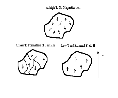
Figure 3: Domain formation during a continuous phase transition: At high temperatures, there is no magnetization. At lower temperatures, individual magnets tend to align with their neighbours creating a local net magnetization, or magnetic domain. The interfaces of the domains move, until the whole sample has the same magnetization. An external magnetic field can bias the direction of the magnetization.

The connection between symmetry breaking in the early Universe and phase transitions has led, during the past 15 years or so, to the emergence of a new interface in physics, namely, that of cosmology and condensed matter physics. Thus, a cosmologist interested in the physics of the early Universe will have to learn techniques from statistical mechanics of phase transitions. Terms like spinodal decomposition and bubble nucleation are now part of the vocabulary of many cosmologists.

What is more important, if phase transitions indeed occurred in the early Universe they would have generated a host of possible observational consequences that not only offer a window to very high energy physics but also may help us solve some of the cosmological problems listed in Section II. Although I won’t be exhaustive here, I hope to give the reader at least a flavour of how this is done in practice. In order to do so, I will concentrate on how ideas from phase transitions can be applied to the resolution of the three challenges to the Big Bang model explained above.

A beautiful and simple description of symmetry breaking in condensed matter physics is presented by the Ginzburg-Landau theory [15]. In order to describe symmetry breaking, one must identify an order parameter, that is, a variable which describes the bulk properties of the system as a given control parameter changes. For example, for the ferromagnet the order parameter may be the net magnetization and the control parameter may be the temperature, or, if we have a mixture of two fluids, the order parameter may be the local concentration difference of the two fluids, and the order parameter the temperature, etc. Order parameters may be scalar functions or complicated matrices, as in the case of ${\rm He}^{3}$. For simplicity, we will restrict ourselves to the simplest possible example (already quite complicated!), that of a scalar order parameter. These models describe liquid-gas transitions, binary fluid mixtures, metal alloys, and Ising ferromagnets, ferromagnets where the spins are restricted to point either up or down with respect to some axis. All these models fall in the so-called Ising universality class, that is, have critical properties which are essentially identical.

For a scalar order parameter, the homogeneous part of the Ginzburg-Landau free energy density is written as

$$V_{\rm GL}(\phi,T)={1\over 2}\alpha(T)\phi^{2}+{{\lambda}\over 4}\phi^{4}-{\cal H}\phi~{}~{},$$

where $\alpha(T)\equiv a(T-T_{c})/T_{c}$ and ${\cal H}$ is an external magnetic field. The similarity with the finite temperature potential for the scalar field is striking! Again, depending on the value of the temperature, $\alpha(T)$ can be positive or negative, being zero at $T_{c}$. The values of the order parameter $\phi$ above and below $T_{c}$ will depend on the external magnetic field ${\cal H}$, as shown in the Figure.

Figure 4: Ginzburg-Landau potentials: Different Ginzburg-Landau potentials for a scalar order parameter are shown without (left) and with (right) an external magnetic field.

The reader can see that there are basically two possible kinds of phase transitions depending on the value of the external field ${\cal H}$. If ${\cal H}=0$, the free energy is symmetric with respect to a $\phi\rightarrow-\phi$ reflection and is simply a degenerate double well. As the temperature drops below $T_{c}$, the order parameter changes continuously between the symmetric $\phi=0$ and the broken-symmetric phase with $\phi^{2}=-\alpha/\lambda$. This is an example of a continuous phase transition, sometimes called a second order phase transition based on an old classification by P. Ehrenfest. The heat capacity $C_{V}=-T\partial^{2}V_{\rm GL}/\partial T^{2}$ has a discontinuity at $T_{c}$.

Continuous phase transitions evolve by spinodal decomposition [16]. Basically, long-wavelength small-amplitude fluctuations grow exponentially fast as domains of the two phases form and compete for dominance. These domains are separated by an interface, where the order parameter changes continuously from one phase to another. Clearly, the order parameter only provides information of the global behavior of the system, leaving aside the complicated local dynamics of the interfaces, a topic of much interest for researchers.

Figure 5: Spinodal Decomposition: The system is initially prepared in thermal equilibrium at $<\phi>=0$. It is then suddently cooled and left to relax to its lowest free energy state. The formation of an interface can be easily seen. [The color PostScript file can be obtained by request from Carmen Gagne at: carmen.gagne@dartmouth.edu]

If the external field $H$ is not zero, the free-energy density will not be degenerate anymore. The presence of the field will bias the system, determining the lowest free energy phase. If the system starts in the highest free energy phase at high temperatures and is rapidly cooled (or quenched) to below $T_{c}$, it will remain trapped in the high free energy phase. In this case, we say that the system is in a metastable phase. The transition to the lowest free energy phase is discontinuous, and occurs through the nucleation of bubbles of the low free energy phase within the metastable phase. This is an example of a discontinuous or first order phase transition. The phenomenon of bubble nucleation is a beautiful illustration of nonlinearities in action; the bubble configuration represents a coherent fluctuation of the field, excited by thermal or quantum effects. We will say more about quantum nucleation below. Let us examine this mechanism in a little more detail.

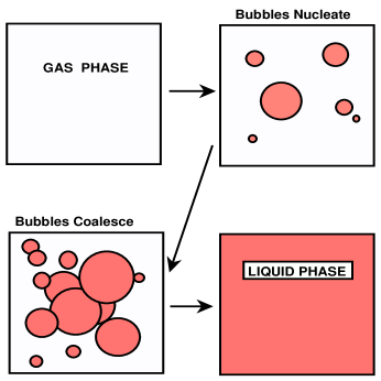
Figure 6: Bubble Nucleation in a discontinuous phase transition: Bubbles from the liquid phase appear inside the gas phase. If they are large enough they grow and percolate, eventually converting the whole volume into the liquid phase.

The energy of a field configuration $\phi_{c}$ is given by

$$E[\phi_{c}]=\int dV\left[{1\over 2}{\vec{\nabla}}\phi_{c}\cdot{\vec{\nabla}}\phi_{c}+V_{\rm GL}(\phi_{c})\right]~{}~{}.$$

It is convenient to analyse the expression for the energy of a thin-wall bubble, that is, a spherically symmetric configuration with a well-defined interior of radius $R$, separated from the exterior by a wall of thickness $L\ll R$. Thus, we can divide the configuration into three parts: the “inside”, where $\phi_{c}={\rm const}=\phi_{+}$; the “outside”, the metastable phase, where $\phi_{c}={\rm const}=\phi_{-}$; and the bubble wall, where the field interpolates between the two minima, $\phi_{\rm w}(x/L)\propto\tanh(x/L)$. Within this approximation we can write, for the energy of a thermally nucleated bubble,

$$E[R]=4\pi\sigma R^{2}-{{4\pi}\over 3}\epsilon R^{3}~{}~{},$$

where $\sigma\equiv(1/2)\int dr{\vec{\nabla}}\phi_{c}\cdot{\vec{\nabla}}\phi_{c}$ is the surface density and $\epsilon\equiv|V_{\rm GL}(\phi_{+},T)-V_{\rm GL}(\phi_{-},T)|$ is the free-energy difference between the two phases. Thus, there is a critical radius $R_{c}=2\sigma/\epsilon$ above which it is favourable for the configuration, or bubble, to grow. If $R<R_{c}$, the surface tension dominates and the bubble shrinks. Note that if $\epsilon=0$, that is, if the two phases are degenerate, $R_{c}\rightarrow\infty$. $R_{c}$ also determines the free energy barrier for the nucleation of the critical bubble, $E[R_{c}]=(16\pi/3)\sigma^{3}/\epsilon^{2}$. The nucleation rate per unit time and unit volume is approximately written as

$$\Gamma\propto T^{4}\exp[-E(R_{c})/T]~{}.$$

If bubbles with $R>R_{c}$ start being nucleated they will grow and coalesce, eventually converting the whole volume of the system from the metastable phase to the lower free energy phase, completing the phase transition. (See Figure 6.)

A similar bubble nucleation mechanism is possible via quantum fluctuations as opposed to thermal fluctuations. The field, trapped in the metastable state, will tunnel to the ground state with a given rate calculated in a similar way. This tunneling is the field theoretical equivalent of the usual barrier penetration mechanism in nonrelativistic quantum mecyhanics, where the wave function has a nonzero probability flow through a potential barrier. As one would expect, the “vacuum decay” rate is smaller than the thermal decay rate, $\Gamma_{\rm vac}\propto m^{4}\exp[-S(R_{c})/\hbar]$, where $S(R_{c})\propto\sigma^{4}/\epsilon^{3}$ and $m$ is the typical mass scale in the problem. $S(R_{c})$ is the four dimensional Euclidean action for the critical bubble configuration, a measure of the barrier for quantum tunneling. Both thermal and quantum bubble nucleation may play a role in the early Universe. Next we will examine how these ideas are applied in the context of early Universe cosmology.

V-Cosmological Phase Transitions

In order to gain some insight into what effects the expansion of the Universe may have in the dynamics of a phase transition, we must first remember that the expansion rate determines how fast the temperature drops compared to the interaction time scale of the particles. From Friedmann’s equations above, the expansion rate of the Universe for a radiation-dominated era is (we can safely take the curvature constant $k=0$ in this regime)

$${{\dot{R}}\over R}=H\simeq 1.66g_{\ast}^{1/2}{{T^{2}}\over{m_{{\rm Pl}}}}~{}~{},$$

where I used that for a relativistic gas in thermal equilibrium at temperature $T$, $\rho={{\pi^{2}}\over{30}}g_{\ast}T^{4}$, where $g_{\ast}$ is the number of relativistic degrees of freedom. A given particle species is in thermal equilibrium in an expanding Universe as long as its interaction rate is faster than the expansion rate, $\Gamma_{\rm int}>H$. With mild assumptions about how particles interact at very high energies, this happens as long as $k_{B}T\leq 10^{16-17}$ GeV [4].

So far I have motivated the discussion of cosmological phase transitions using only the electroweak phase transition as an example. Now, I would like to discuss another phase transition which may have ocurred much earlier than the electroweak symmetry breaking. This is a phase transition related to the breaking of the symmetry described by the so-called Grand Unified Theory (GUT), where the strong interaction is unified with the electroweak interaction [17]. Current estimates of when this unification occurs lead to an energy scale of about $10^{16}$ GeV, roughly 14 orders of magnitude above the electroweak unification. In the context of the Big Bang model, such energies were achieved when the Universe was about $10^{-38}$ sec old.

If a phase transition indeed happened at this early time, it would have left some very interesting signatures. One of them, which will be treated in future articles by A. Gill and T. Vachaspati in this magazine, is the possibility that the transition generated certain “energy knots” in the field configurations, known as topological defects. The various types of topological defects are determined by the kind of symmetry that is broken, which in turn depends on the details of the unification scheme. For example, if a discrete (left-right) symmetry is broken as in the simple GL model above, sheet-like defects known as “domain walls” or interfaces would appear between the two phases [18].

These topological defects are both a blessing and a curse for cosmologists. Curse because some of them may dominate the energy density of the Universe and cause an expansion rate different from the observed one. Domain walls would create an ultra fast expansion rate, where the scale factor would expand as $R\propto t^{2}$ [19]. This expansion rate would lead to severe discrepancies with observations, for example the abundance of light elements predicted from nucleosynthesis. Thus, cosmology rules out this kind of symmetry breaking at the GUT scale, a beautiful example of how it can influence particle physics. (Unless, of course, the left-right symmetry is not exact…) Blessing because these topological defects may play a role in the formation of large-scale structure, although models are becoming increasingly constrained by observations of the cosmic background radiation.

But here I want to explore another possible consequence of the GUT-scale phase transition, known as the inflationary cosmology, as it exemplifies very clearly the interplay between cosmology and the dynamics of phase transitions. Since the original model proposed by the American physicist Alan Guth in 1981, the idea of inflation has mutated into several different scenarios, some of them not invoking directly a GUT-scale symmetry breaking [20]. However, in this author’s opinion, these various scenarios are viability studies which indicate how a larger theory related to unification at high energy scales will be applied to cosmology. With this said, I move on to explain the basic mechanism of inflation, starting with Guth’s original model.

In Guth’s model, the effective potential responsible for the breaking of the GUT symmetry had a metastable phase. As the Universe expanded and cooled, the scalar field responsible for the symmetry breaking became trapped in this metastable state. In this case, at high enough temperatures, the energy density of all matter would have two terms, one from relativistic radiation and one from the vacuum energy,

$$\rho={{\pi^{2}}\over{30}}g_{\ast}T^{4}+V_{0}~{}~{},$$

where $V_{0}$ is the constant energy density of the field while trapped in the metastable minimum. Clearly, when the temperature $T<\left(30V_{0}/g_{\ast}\pi^{2}\right)^{1/4}$, the energy density will be dominated by the constant vacuum energy, and, as we saw in Section 1, the scale factor will expand exponentially fast, $R\propto{\rm exp}(\sqrt{\Lambda_{\rm vac}}t)$. Hence the name inflation. While the scalar field is trapped in this metastable phase, the Universe will expand superluminally and become supercooled. [Note that this doesn’t mean that information will be travelling faster than the speed of light. Particles, and their interactions, will still obey causality.] Due to the sudden drop in temperature, quantum effects will dominate over thermal effects. Eventually, the field will decay into the lowest energy state by the mechanism of quantum bubble nucleation. These bubbles will grow and coalesce, completing the phase transition.

The problem with this original scenario, now called “old inflation”, is that the bubbles’s growth rate, which is determined by causal processes, can not compete with the exponential expansion rate of the Universe; the bubbles can not meet and coalesce to complete the phase transition. Many alternatives have been proposed since then, with names like new inflation, chaotic inflation, extended inflation, natural inflation, etc. In one way or another, all scenarios for inflation rely on the extra potential energy available as a given scalar field (or fields) approaches its final low energy state, be it through bubble nucleation, or by rolling down its potential. At this point it is fair to say that we understand what are the desirable and undesirable consequences of an inflationary epoch in the early Universe, although we are still lacking a truly compelling model. Information coming from GUT-scale particle physics and from the cosmic microwave background would be most welcome here.

What are the benefits of an inflationary phase? First, if there are any unwanted relics from the phase transition, such as undesirable topological defects, these would be “inflated away”, that is, their number density would decrease to a negligible and harmless amount. Second, for a sufficiently long inflationary expansion, a small causally connected volume could have grown to encompass the whole of the observed Universe today. In this case, the smoothness problem of the Big-Bang model could be solved (see Figure 7).

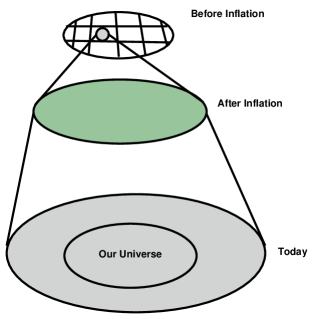
Figure 7: Smoothness problem solved by inflation: Due to the exponentially fast expansion during inflation, a small, causally-connected patch (shown in grey) can grow to encompass our whole visible Universe.

In order to solve the smoothness problem, the scale factor must grow by about 30 orders of magnitude during inflation, such that a length scale which before inflation was $10^{-28}{\rm cm}$ would be “stretched” to $10^{2}{\rm cm}$ by the end of inflation. Today, this length scale would correspond to $10^{28}{\rm cm}$, roughly the size of the observable Universe. The important point is that before inflation, length scales smaller than $10^{-24}{\rm cm}$ were causally connected. Thus, our whole observable Universe would have fitted quite comfortably within a causally connected patch!

A second benefit from the inflationary model is that it can also provide a mechanism to generate the seeds that will be ultimately responsible for the observed large-scale structure of the Universe. As we know from basic quantum mechanics, the zero-point energy of a quantum system indicates the presence of fluctuations about the classical minimum of energy. An example is the simple harmonic oscillator in the position representation. As we move on to fields, the vacuum will also be populated by zero point fluctuations of different wavelengths. Since during inflation length scales are stretched exponentially fast ($R\propto{\rm exp}(\sqrt{\Lambda_{\rm vac}}t)$, while the Hubble radius ($D_{H}(t)=H(t)^{-1}=R/{\dot{R}}$) remains constant, it is possible for a perturbation of a given length scale to grow bigger than the Hubble radius during inflation and then reenter it at a later time during the radiation or the matter dominated eras (see Figure 8). Thus, inflation offers a mechanism of amplification of quantum fluctuations into the density perturbations which will cause the gravitational instabilities needed for structure formation later on in the evolution of the Universe.

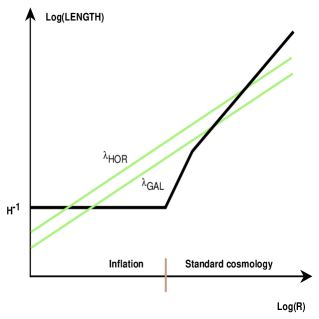
Figure 8: Perturbations reentering causally connected horizon: During inflation, perturbations of both galactic ($\lambda_{\rm GAL}$) and horizon scale ($\lambda_{\rm HOR}$) are stretched outside causally-connected regions defined by the Hubble radius ($H^{-1}$). As inflation ends, the Universe enters a radiation-dominated era, followed by a matter-dominated era, grouped jointly in the figure as “standard cosmology”. During the standard cosmology era, the perturbations grow slower than the Hubble radius and will eventually reenter the causally-connected Universe, generating the perturbations responsible for large-scale structures of different sizes.

Finally, we will examine how the third of the challenges to the Big Bang model we mentioned earlier, that of the excess of matter over anti-matter, can be solved by a primordial phase transition. There are several mechanisms for generating the matter (or baryonic) excess, either during the GUT phase transition or the electroweak phase transition. However, here we will focus more on electroweak baryogenesis as it calls for physics of much lower energy scales. The basic ideas, applicable to both situations, were presented in a pioneer work by A. Sakharov in 1968. [The reader interested in more details should consult the article by M. Shaposhnikov dedicated to electroweak baryogenesis.]

Sakharov suggested that three conditions must be satisfied in order to produce the matter excess; first, there must be a way of creating both more baryons and anti-baryons. Then, there must be a mechanism to bias the creation of more baryons than anti-baryons. And finally, once we have an excess of matter particles over their anti-matter partners, we must make sure that this excess is not erased as the Universe continues to expand [10, 11].

The first of these conditions is the creation of both baryons and anti-baryons from collisions involving the other particles present in the primordial soup. At low energies, the number of baryons participating in collisions between different particles is conserved, that is, just like electric charge, the total number of baryons before an interaction equals the total after. If we are interested in making baryons, as we must in order to create matter in the Universe, this conservation law is not very useful. According to Sakharov’s requirement, however, at very high energies the interactions between elementary particles should not conserve the number of baryons. This is both true from the decay of heavy GUT-scale particles and from the non-trivial vacuum structure of the electroweak theory, which has degenerate minima with different baryon number, as shown in Figure 9.

But this first condition does not differentiate between baryons and anti-baryons. At high temperatures we could still create the same number of each, and that wouldn’t cause a bias toward matter over anti-matter. We need a second condition. Once the high energies of the early Universe allow for the creation of baryons and anti-baryons, we need a condition that selects, or biases, the creation of baryons over anti-baryons, an arrow pointing in the right direction (i.e., toward baryons). This is known as CP violation, from the operations of charge conjugation and parity, familiar from quantum mechanics. In 1964, J.H. Christenson and collaborators found experimental evidence that interactions between certain baryons do indeed exhibit this bias. It is as if Nature has its own biases, in this case toward more baryons. If this is true in laboratory experiments, no doubt this will also be true in the early Universe.

Finally, once we have produced a net baryonic excess, we must ensure that it will not go away. This leads to the third Sakharov condition, that baryogenesis requires the Universe to be out of thermal equilibrium. We can understand the need for this condition with the following illustration.

Hot systems have no memory of their past. Imagine a coffee spoon which is initially cold. Now immerse one of its ends into a very hot cup of coffee. What happens? Although early on only the end in the coffee will be hot, very quickly the whole spoon will be equally hot. You won’t be able to tell which of the two ends was immersed into the coffee cup; the system (coffee spoon and hot coffee) lost its “memory”. Another term for this loss of memory is thermal equilibrium. If the early Universe was in thermal equilibrium, any excess baryons would have been deleted; in equilibrium, the net baryon number is zero. In order to maintain the baryon bias as the Universe cools, we need to make sure the Universe doesn’t “lose it’s memory” and delete the new baryons. We need out of equilibrium conditions.

In GUT-scale baryogenesis out of equilibrium conditions are achieved by the irreversible decays of heavy particles. Due to the expansion of the Universe, the reaction rate of processes involving the decays of a heavy particle into lighter ones won’t be able to keep up with the expansion rate of the Universe. Roughly, the expansion makes it hard for the lighter particles to meet and keep the reaction going both ways. [$X\rightarrow q_{i}+{\bar{q}_{j}}$, where $q_{i}$ and $q_{j}$ are two lighter particles.]

In electroweak baryogenesis, the idea is to use the dynamics of the phase transition to generate the excess baryon number. It is clear that a phase transition always involve out of equilibrium conditions: whenever the system finds itself in a higher free energy density phase, it will relax into the lowest possible free energy phase. Most mechanisms of electroweak baryogenesis assume a typical discontinuous phase transition via the usual bubble nucleation mechanism.

In the symmetric high temperature phase, baryon number is freely violated with a rate proportional to $T^{4}$. However, in the broken-symmetric, low-temperature phase, this rate is suppresed by a Boltzmann factor, $\Gamma_{\rm b-viol}\propto\exp{[-E_{\rm sph}/T]}$, where $E_{\rm sph}$ is the energy of the so-called sphaleron configuration (from the Greek “ready to fall”), which interpolates between vacua of different baryon number (see Figure 9). Thus, the excess baryons are generated in the symmetric phase.

Figure 9: Baryon number violation in the electroweak theory: The nontrivial vacuum of the electroweak theory allows for degenerate minima with different baryon number. Thus, jumping from one vacuum to another it is possible to generate the baryon number excess. The field configuration responsible for the interpolation between different vacua at high enough temperatures is the sphaleron. At very high temperatures, higher than the barrier shown, the baryon number violation rate is simply proportional to $T^{4}$.

As the Universe expands and cools, bubbles of the broken-symmetric phase form inside the symmetric phase. The excess baryons “cooked” in the symmetric phase have a probability of going through the bubble wall, generating a net baryon number excess inside the bubble. Since inside the growing bubbles baryon number is conserved (up to exponential accuracy), this net excess survives and becomes the matter we are ultimately made of. (See Figure 10.)

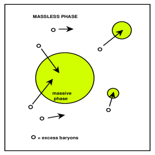
Figure 10: Schematics of electroweak baryogenesis: In the symmetric massless phase baryon number is violated, while in the massive broken symmetric phase baryon number is conserved. The excess baryons generated in the massless phase will penetrate the bubbles, generating the excess baryon number in the Universe.

There have been several different versions of electroweak baryogenesis in the past five years or so, motivated mostly by the difficulty of generating the right amount of CP violation in the Standard Model of particle physics. These so-called extensions to the Standard Model come in many different flavours, but are usually able to generate a much larger amount of CP violation and thus of baryonic excess, even if at the cost of introducing more arbitrary parameters. On the other hand, one could argue that electroweak baryogenesis calls for physics beyond the Standard Model, another beautiful illustration of the cosmology/particle physics interface implemented through cosmological phase transitions.

Although much progress has been made in our understanding of the dynamics of cosmological phase transitions and their impact on the history of the Universe, it should be clear that the future of this field is still quite open. As this author has shown in a series of articles, the use of typical bubble nucleation mechanisms to describe these transitions may be naive, the truth lying somewhere in between the two “archetypes” of continuous and discontinuous phase transitions [21, 22]. Since cosmological phase transitions are the main link between micro and macro physics, we should expect many surprises in the years to come.

References

- [1] A general overview of the history of cosmological ideas from the Greeks to the Big Bang can be found in M. Gleiser, The Dancing Universe: From Creation Myths to the Big Bang, (Dutton, New York, 1997).
- [2] E. P. Hubble, Proc. Nat. Acad. Sci, 15, (1929) 168; Ap. J., 71, (1930) 231.
- [3] W. de Sitter, Mon. Not. Roy. Astron. Soc., 78, (1917) 3; A. Friedmann, Z. Phys., 10, (1922) 377; ibid., 21, (1924) 326; G. Lemaître, Ann. Soc. Sci. Brux., A47, (1927) 49; Mon. Not. Roy. Astron. Soc., 141, (1931) 483.
- [4] For a more technical overview of modern cosmology see, e.g., E. W. Kolb and M. S. Turner, The Early Universe (Addison-Wesley, New York, 1990).
- [5] G. Gamow, Phys. Rev., 70, (1946) 572; R. A. Alpher, H. Bethe, and G. Gamow, Phys. Rev., 73, (1948) 803; G. Gamow, Phys. Rev. 74, (1948) 505; R. A. Alpher and R. C. Hermann, Nature, 162, (1948) 774; R. A. Alpher, R. C. Hermann, and G. Gamow, Phys. Rev., 74, (1948) 1198; R. A. Alpher and R. C. Hermann, Rev. Mod. Phys., 22, (1950) 153.
- [6] For an account of nucleosynthesis for the general audience see, L. Lederman and D. Schramm, From Quarks to the Cosmos (Scientific American Library, New York, 1989).
- [7] A. A. Penzias and R. W. Wilson, Ap. J., 142, (1965) 419; R. H. Dicke, P. J. E. Peebles, P. G. Roll, and D. T. Wilkinson, Ap. J., 142, (1965) 414.
- [8] For a review with an excellent list of references see L. Page in Critical Dialogues in Cosmology, ed. N. Turok (World Scientific, Singapore, 1997). For a popular account of the discovery and history of the microwave background see S. Weinberg, The First Three Minutes, (Basic Books, New York, 1977).
- [9] L. N. da Costa, M. J. Geller, P. S. Pellegrini, D. W. Latham et al., Ap. J. Lett., 424, (1994) L1. See also the review by M. Davis in Critical Dialogues in Cosmology, ed. N. Turok (World Scientific, Singapore, 1997).
- [10] A. G. Cohen, D. B. Kaplan, and A. E. Nelson, Annu. Rev. Nucl. Part. Sci., 43, 27 (1993); A. Dolgov, Phys. Rep., 222, 311 (1992). For a popular account of the matter/anti-matter problem, see, M. Gleiser’s contribution to the internet text of the BBC series Stephen Hawking’s Universe at http://www.pbs.org.
- [11] M. Gleiser, in The Birth of the Universe and Fundamental Physics, ed. F. Occhionero (Kluger, XXXX, 1996).
- [12] For a technical account see, C. Quigg, Gauge Theories of the Strong, Weak, and Electromagnetic Interactions (Benjamin/Cummings, Reading, MA, 1983).
- [13] L. H. Ryder, Quantum Field Theory, (Cambridge University Press, Cambridge, 1985).
- [14] For a technical review of phase transitions see, J. D. Gunton, M. San Miguel and P. S. Sahni, in Phase Transitions and Critical Phenomena, Vol. 8, Ed. C. Domb and J. L. Lebowitz (Academic Press, London, 1983).
- [15] See for example, N. Goldenfeld, Lectures on Phase Transitions and the Renormalization Group, Frontiers in Physics, Vol. 85, (Addison-Wesley, 1992).
- [16] J. S. Langer, Physica 73, 61 (1974); Ann. Phys. (NY) 41, 108 (1967); 54, 258 (1969).
- [17] G. G. Ross, Grand Unified Theories (Benjamin/Cummings, Reading, MA, 1984).
- [18] T. W. B. Kibble, J. Phys., A9, (1976) 1387. For reviews see M. B. Hindmarsh and T. W. B. Kibble, Rep. Prog. Phys., 55, (1995) 478; A. Vilenkin and E. P. S. Shellard, Cosmic Strings and Other Topological Defects, (Cambridge University Press, Cambridge, 1994).
- [19] G. Gelmini, M. Gleiser, and E. W. Kolb, Phys. Rev. D39, (1989) 1558.
- [20] A. H. Guth, Phys. Rev., D 23, (1981) 347; For a recent debate of the status of the inflationary universe see the contributions by A. H. Guth, W. Unruh, and A. Albrecht in, Critical Dialogues in Cosmology, ed. N. Turok (World Scientific, Singapore, 1997); For a popular account of inflation see, A. Guth, The Inflationary Universe (Addison-Wesley, New York, 1997).
- [21] M. Gleiser, E. W. Kolb, and R. Watkins, Nucl. Phys., B364, (1991) 411; G. Gelmini and M. Gleiser, Nucl. Phys., B419, (1994) 129; M. Gleiser and E. W. Kolb, Phys. Rev. Lett., 69, (1992) 1304; A. Heckler and M. Gleiser, Phys. Rev. Lett., 76, (1996) 180; M. Gleiser, A. Heckler, and E.W. Kolb, Phys. Lett., B405 (1997) 121.
- [22] M. Gleiser, Phys. Rev. Lett., 73, (1994) 3495; J. Borrill and M. Gleiser, Phys. Rev., D51, (1995) 4111; J. Borrill and M. Gleiser, Nucl. Phys. B483, (1997) 416.