KA-TP-2-1998
hep-ph/9803277
QCD Corrections to the Masses of the neutral ${\cal CP}$-even Higgs Bosons in the MSSM

Abstract

We perform a diagrammatic calculation of the leading two-loop QCD corrections to the masses of the neutral ${\cal CP}$-even Higgs bosons in the Minimal Supersymmetric Standard Model (MSSM). The results are valid for arbitrary values of the parameters of the Higgs and scalar top sector of the MSSM. The two-loop corrections are found to reduce the mass of the lightest Higgs boson considerably compared to its one-loop value. The numerical results are analyzed in the GUT favored regions of small and large $\tan\beta\hskip 2.84526pt$. Their impact on a precise prediction for the mass of the lightest Higgs boson is briefly discussed.

Supersymmetric theories (SUSY) [1] are the best motivated extensions of the Standard Model (SM) of the electroweak and strong interactions. They provide an elegant way to break the electroweak symmetry and to stabilize the huge hierarchy between the GUT and the Fermi scales, and allow for a consistent unification of the gauge coupling constants as well as a natural solution of the Dark Matter problem; for recent reviews see Ref. [2]. The MSSM predicts the existence of scalar partners $\tilde{f}_{L},\tilde{f}_{R}$ to each SM chiral fermion, and spin-$1/2$ partners to the gauge bosons and to the scalar Higgs bosons. So far, the direct search for SUSY particles has not been successful. One can only set lower bounds of ${\cal O}(100)\,\,{\mathrm{G}eV}$ on their masses [3].

A particularly stringent test of the MSSM is the search for the lightest Higgs boson. At tree level its mass, $m_{h}$, is predicted to be lower than the one of the $Z$ boson. However, the one-loop corrections are known to be huge [4, 5]. As an impact, $m_{h}>M_{Z}$ is possible, and an upper bound of approximately $150\,\,{\mathrm{G}eV}$ is obtained. Hence a two-loop calculation is inevitable for a precise prediction of the mass of the lightest Higgs boson. This is particularly important in view of the search for this particle at LEP2, where a precise knowledge of $m_{h}$ in terms of the relevant SUSY parameters is crucial in order to determine the discovery (and of course also the exclusion) potential of LEP2.

Up to now there exist renormalization group improvements of the one-loop result by including the two-loop leading logarithmic contributions [6, 7, 8], and a diagrammatic calculation of the dominant two-loop contributions in the limiting case of vanishing $\tilde{t}$-mixing and infinitely large $M_{A}$ and $\tan\beta\hskip 2.84526pt$ [9]. These results indicate that the two-loop corrections considerably reduce the prediction for $m_{h}$. However, a diagrammatic two-loop calculation of the neutral mass spectrum going beyond the above-mentioned limiting case has been missing so far. Such a Feynman diagrammatic calculation is technically very involved, but it is of particular interest since it allows for general parameters of the MSSM Higgs sector and for virtual particle effects without restrictions on their masses and mixing. It is the purpose of this letter to investigate the leading QCD corrections to the masses of the neutral ${\cal CP}$-even Higgs bosons and in particular to provide in this way a two-loop prediction of $m_{h}$ for arbitrary values of the parameters of the Higgs and scalar top sector of the MSSM.

Contrary to the SM, in the MSSM two Higgs doublets are needed. The Higgs potential is given by [10]

$$V= m_{1}^{2}H_{1}\bar{H}_{1}+m_{2}^{2}H_{2}\bar{H}_{2}-m_{12}^{2}(\epsilon_{ab}H_{1}^{a}H_{2}^{b}+\mbox{h.c.})$$ (1)

$$+ \frac{g^{\prime 2}+g^{2}}{8}\,(H_{1}\bar{H}_{1}-H_{2}\bar{H}_{2})^{2}+\frac{g^{2}}{2}\,|H_{1}\bar{H}_{2}|^{2},$$ (2)

where $m_{1},m_{2},m_{12}$ are soft SUSY-breaking terms, $g,g^{\prime}$ are the $SU(2)$ and $U(1)$ gauge couplings, and $\epsilon_{12}=-1$.

The doublet fields $H_{1}$ and $H_{2}$ are decomposed in the following way:

$$H_{1} = \left(\begin{array}[]{c}H_{1}^{1}\\ H_{1}^{2}\end{array}\right)=\left(\begin{array}[]{c}v_{1}+(\phi_{1}^{0}+i\chi_{1}^{0})/\sqrt{2}\\ \phi_{1}^{-}\end{array}\right),$$ (7)

$$H_{2} = \left(\begin{array}[]{c}H_{2}^{1}\\ H_{2}^{2}\end{array}\right)=\left(\begin{array}[]{c}\phi_{2}^{+}\\ v_{2}+(\phi_{2}^{0}+i\chi_{2}^{0})/\sqrt{2}\end{array}\right).$$ (12)

The potential eq. (1) can be described with the help of two independent parameters (besides $g$, $g^{\prime}$): $\tan\beta\hskip 2.84526pt=v_{2}/v_{1}$ and $M_{A}^{2}=-m_{12}^{2}(\tan\beta\hskip 2.84526pt+\cot\beta\hskip 2.84526pt)$, where $M_{A}$ is the mass of the ${\cal CP}$-odd $A$ boson.

At tree level the mass matrix of the neutral ${\cal CP}$-even Higgs bosons is given in the $\phi_{1}-\phi_{2}$ basis in terms of $M_{Z}$ and $M_{A}$ through

$$M_{\rm Higgs}^{2,{\rm tree}}=\left(\begin{array}[]{cc}m_{\phi_{1}}^{2}&m_{\phi_{1}\phi_{2}}^{2}\\ m_{\phi_{1}\phi_{2}}^{2}&m_{\phi_{2}}^{2}\end{array}\right)=$$ (15)

$$\left(\begin{array}[]{cc}M_{A}^{2}\sin^{2}\beta\hskip 2.84526pt+M_{Z}^{2}\cos^{2}\beta&-(M_{A}^{2}+M_{Z}^{2})\sin\beta\hskip 2.84526pt\cos\beta\\ -(M_{A}^{2}+M_{Z}^{2})\sin\beta\hskip 2.84526pt\cos\beta&M_{A}^{2}\cos^{2}\beta\hskip 2.84526pt+M_{Z}^{2}\sin^{2}\beta\end{array}\right).$$ (18)

The tree-level mass predictions receive large corrections at one-loop order through terms proportional to $G_{F}m_{t}^{4}\ln(m_{\tilde{t}_{1}}m_{\tilde{t}_{2}}/m_{t}^{2})$ [4]. These dominant one-loop contributions can be obtained by evaluating the contribution of the $t-\tilde{t}$-sector to the $\phi_{1,2}$ self-energies at zero external momentum from the Yukawa part of the theory (neglecting the gauge couplings). Accordingly, the one-loop corrected Higgs masses are derived by diagonalizing the mass matrix

$$M^{2}_{\rm Higgs}=\left(\begin{array}[]{c}m_{\phi_{1}}^{2}-\hat{\Sigma}_{\phi_{1}}(0)\;\;\;\;\;\;m_{\phi_{1}\phi_{2}}^{2}-\hat{\Sigma}_{\phi_{1}\phi_{2}}(0)\\ m_{\phi_{1}\phi_{2}}^{2}-\hat{\Sigma}_{\phi_{1}\phi_{2}}(0)\;\;\;\;\;\;m_{\phi_{2}}^{2}-\hat{\Sigma}_{\phi_{2}}(0)\end{array}\right),$$ (19)

where the $\hat{\Sigma}$ denote the Yukawa contributions of the $t-\tilde{t}$-sector to the renormalized one-loop $\phi_{1,2}$ self-energies. By comparison with the full one-loop result [5] it has been shown that these contributions indeed contain the bulk of the one-loop corrections. They typically approximate the full one-loop result up to about 5 GeV.

In order to derive the leading two-loop contributions to the masses of the neutral ${\cal CP}$-even Higgs bosons we have evaluated the QCD corrections to eq. (19), which because of the large value of the strong coupling constant are expected to be the most sizable ones (see also Ref. [9]). This requires the evaluation of the renormalized $\phi_{1,2}$ self-energies at the two-loop level. Typical Feynman diagrams corresponding to the Yukawa contributions of the $t-\tilde{t}$-sector to the $\phi_{1,2}$ self-energies and tadpoles are shown in Fig. 1. They have to be supplemented by the counterterm insertions in the corresponding one-loop diagrams. Fig. 1a shows the pure scalar contributions to the Higgs self-energies. In Fig. 1b the gluonic corrections are depicted, while Fig. 1c shows the gluino-exchange contribution. In Fig. 1d-f the tadpole contributions for these three types of corrections are given.

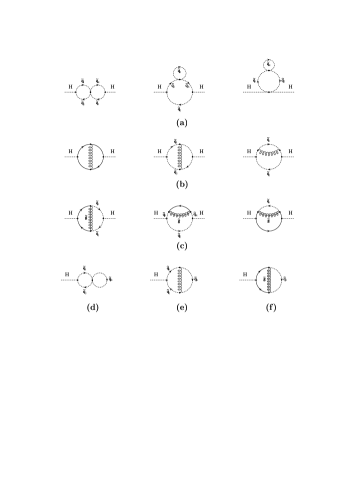
FIG. 1.: Typical Feynman diagrams for the two-loop contribution to the Higgs-boson self-energies and tadpoles. $H=\phi_{1},\phi_{2},A$.

The renormalization has been performed in the on-shell scheme. The counterterms in the Higgs sector are derived from the Higgs potential eqs. (1), (12) by expanding the counterterm contributions up to two-loop order. The renormalization conditions for the tadpole counterterms have been chosen in such a way that they cancel the tadpole contributions in one- and two-loop order. The renormalization in the $t-\tilde{t}$-sector has been performed in the same way as in Ref. [11]. For the present calculation the one-loop counterterms $\delta m_{t}$, $\delta m_{\tilde{t}_{1}}$, $\delta m_{\tilde{t}_{2}}$ for the top-quark and scalar top-quark masses and $\delta\theta_{\tilde{t}}$ for the mixing angle contribute, which enter via the subloop renormalization. The appearance of the $\tilde{t}$ mixing angle $\theta_{\tilde{t}}$ reflects the fact that the current eigenstates, $\tilde{t}_{L}$ and $\tilde{t}_{R}$, mix to give the mass eigenstates $\tilde{t}_{1}$ and $\tilde{t}_{2}$. Since the non-diagonal entry in the scalar quark mass matrix is proportional to the quark mass the mixing is particularly important in the case of the third generation scalar quarks. The mixing-angle counterterm $\delta\theta_{\tilde{t}}$ is chosen such that there is no mixing between $\tilde{t}_{1}$ and $\tilde{t}_{2}$ when $\tilde{t}_{1}$ is on-shell. The numerical result, however, is insensitive to this choice of the renormalization point. The one-loop counterterms for $\mu$ and $\tan\beta\hskip 2.84526pt$, $\delta\mu$ and $\delta\tan\beta\hskip 2.84526pt$, do not contribute since they are independent of $\alpha_{s}$.

The renormalized self-energies have the following structure:

$$\hat{\Sigma}_{s}(0)=\Sigma^{(1)}_{s}(0)+\Sigma^{(2)}_{s}(0)-\delta V_{s}^{(1)}-\delta V_{s}^{(2)},$$ (20)

where $s=\phi_{1},\phi_{2},\phi_{1}\phi_{2}$. $\Sigma^{(1)}_{s}$ and $\Sigma^{(2)}_{s}$ denote the unrenormalized self-energies at the one- and two-loop level, and $\delta V^{(1)}_{s}$ and $\delta V^{(2)}_{s}$ are the one- and two-loop counterterms derived from the Higgs potential. The counterterms read:

$$\delta V_{\phi_{1}}^{(i)} = +\delta M_{A}^{2(i)}\sin^{2}\beta\hskip 2.84526pt-\delta t_{1}^{(i)}\frac{e\,\cos\beta\hskip 2.84526pt}{2M_{W}s_{W}}(1+\sin^{2}\beta\hskip 2.84526pt)$$ (22)

$$+\delta t_{2}^{(i)}\frac{e}{2M_{W}s_{W}}\cos^{2}\beta\hskip 2.84526pt\sin\beta\hskip 2.84526pt,$$

$$\delta V_{\phi_{2}}^{(i)} = +\delta M_{A}^{2(i)}\cos^{2}\beta\hskip 2.84526pt-\delta t_{2}^{(i)}\frac{e\,\sin\beta\hskip 2.84526pt}{2M_{W}s_{W}}(1+\cos^{2}\beta\hskip 2.84526pt)$$ (24)

$$+\delta t_{1}^{(i)}\frac{e}{2M_{W}s_{W}}\sin^{2}\beta\hskip 2.84526pt\cos\beta\hskip 2.84526pt,$$

$$\delta V_{\phi_{1}\phi_{2}}^{(i)} = -\delta M_{A}^{2(i)}\sin\beta\hskip 2.84526pt\cos\beta\hskip 2.84526pt-\delta t_{1}^{(i)}\frac{e}{2M_{W}s_{W}}\sin^{3}\beta\hskip 2.84526pt$$ (26)

$$-\delta t_{2}^{(i)}\frac{e}{2M_{W}s_{W}}\cos^{3}\beta\hskip 2.84526pt,$$

with $\delta t_{a}^{(i)}=-T_{a}^{(i)}$, where $T_{a}^{(i)}$ denotes the tadpole contribution, $\delta t_{a}^{(i)}$ is the corresponding counterterm, and $\delta M_{A}^{2(i)}=\Sigma_{A}^{(i)}(0)$ ($i=1,2$).

In deriving our results we have made strong use of computer-algebra tools. The package FeynArts [12] (in which the relevant part of the MSSM has been implemented) has been applied to generate the Feynman amplitudes and the counterterm contributions. For evaluating the amplitudes the package TwoCalc [13] has been used. The calculations have been performed using Dimensional Reduction (DRED) [14], which is necessary in order to preserve the relevant SUSY relations. Naive application (without an appropriate shift in the couplings) of Dimensional Regularization (DREG) [15], on the other hand, does not lead to a finite result. The same observation has also been made in Ref. [9].

The contributions of the scalar, the gluon-, and the gluino-exchange diagrams in Fig. 1 together with the corresponding counterterm contributions are not separately finite (as it was the case in the calculation of Ref. [11]), but have to be combined in order to obtain a finite result. Our results for the two-loop $\phi_{1,2}$ self-energies are given in terms of the SUSY parameters $\tan\beta\hskip 2.84526pt$, $M_{A}$, $\mu$, $m_{\tilde{t}_{1}}$, $m_{\tilde{t}_{2}}$, $\theta_{\tilde{t}}$, and $m_{\tilde{g}}$. In the general case the results are by far too lengthy to be given here explicitly. In the special case of vanishing mixing in the $\tilde{t}$-sector, $\mu=0$, and $m_{\tilde{t}_{1}}=m_{\tilde{t}_{2}}=m_{\tilde{t}}$, a relatively compact expression can be derived. It is given by

$$\hat{\Sigma}^{(2)}_{\phi_{1}}(0)=0,\;\;\;\;\;\hat{\Sigma}^{(2)}_{\phi_{1}\phi_{2}}(0)=0$$ (27)

$$\hat{\Sigma}^{(2)}_{\phi_{2}}(0)=\frac{G_{F}\sqrt{2}}{\pi^{2}}\frac{\alpha_{s}}{\pi}\frac{m_{t}^{2}}{\sin^{2}\beta\hskip 2.84526pt}\Bigg{\{}\left(m_{\tilde{t}}^{2}-m_{\tilde{g}}^{2}-m_{t}^{2}\right)\cdot$$ (38)

$$\Big{[}(1+\frac{m_{t}^{2}}{m_{\tilde{t}}^{2}})-\Big{(}\mbox{Re}\,B_{0}^{fin}(m_{t}^{2},m_{\tilde{g}},m_{\tilde{t}})\left(1-2L\right)$$

$${}+\mbox{Re}\,B_{0}^{fin}(m_{\tilde{t}}^{2},m_{\tilde{g}},m_{t})\frac{m_{t}^{2}}{m_{\tilde{t}}^{2}}\Big{)}$$

$${}-\frac{m_{\tilde{g}}^{2}}{m_{\tilde{t}}^{2}\,N}\left(m_{\tilde{g}}^{2}(m_{\tilde{t}}^{2}+m_{t}^{2})-(m_{\tilde{t}}^{2}-m_{t}^{2})^{2}\right)\ln\left(m_{\tilde{g}}^{2}\right)$$

$${}+\frac{4}{N^{2}}m_{\tilde{g}}^{4}m_{t}^{2}\Phi(m_{t},m_{\tilde{t}},m_{\tilde{g}})\Big{]}-2m_{\tilde{g}}^{2}\ln\left(m_{\tilde{g}}^{2}\right)L$$

$${}+(2m_{\tilde{t}}^{2}+m_{t}^{2})\ln\left(m_{\tilde{t}}^{2}\right)L-3m_{t}^{2}\ln\left(m_{t}^{2}\right)\ln\left(m_{\tilde{t}}^{2}\right)$$

$${}+\frac{1}{N}\ln\left(m_{\tilde{t}}^{2}\right)\Big{[}2m_{\tilde{g}}^{6}-m_{\tilde{g}}^{4}(7m_{\tilde{t}}^{2}+m_{t}^{2})+4m_{\tilde{g}}^{2}(2m_{\tilde{t}}^{4}$$

$${}-3m_{\tilde{t}}^{2}m_{t}^{2}-3m_{t}^{4})-(3m_{\tilde{t}}^{2}-7m_{t}^{2})(m_{\tilde{t}}^{2}-m_{t}^{2})^{2}\Big{]}$$

$${}+3m_{t}^{2}\ln^{2}\left(m_{t}^{2}\right)+\frac{1}{m_{\tilde{t}}^{2}N}\ln\left(m_{t}^{2}\right)\Big{[}2m_{\tilde{t}}^{2}(m_{\tilde{t}}^{2}-m_{\tilde{g}}^{2})^{3}$$

$${}-m_{\tilde{t}}^{2}m_{t}^{2}(5m_{\tilde{g}}^{4}-16m_{\tilde{g}}^{2}m_{\tilde{t}}^{2}+11m_{\tilde{t}}^{4})+m_{t}^{4}(17m_{\tilde{t}}^{4}$$

$${}+6m_{\tilde{g}}^{2}m_{\tilde{t}}^{2}-m_{\tilde{g}}^{4})-9m_{\tilde{t}}^{2}m_{t}^{6}+m_{t}^{8}\Big{]}\Bigg{\}},$$

with $L=\ln(m_{\tilde{t}}^{2}/m_{t}^{2})$, and

$$N=\left((m_{\tilde{g}}-m_{t})^{2}-m_{\tilde{t}}^{2}\right)\left((m_{\tilde{g}}+m_{t})^{2}-m_{\tilde{t}}^{2}\right),$$ (39)

$$\Phi(x,y,z)=\frac{1}{2}z^{2}\lambda\left(\frac{x^{2}}{z^{2}},\frac{y^{2}}{z^{2}}\right)\Big{[}2\ln(\alpha^{1}_{xyz})\ln(\alpha^{2}_{xyz})$$ (40)

$${}-\ln\left(\frac{x^{2}}{z^{2}}\right)\ln\left(\frac{y^{2}}{z^{2}}\right)-2{\rm Li_{2}}(\alpha^{1}_{xyz})-2{\rm Li_{2}}(\alpha^{2}_{xyz})+\frac{\pi^{2}}{3}\Big{]},$$ (41)

$$\lambda(u,v)=\sqrt{1+u^{2}+v^{2}-2u-2v-2uv},$$ (42)

$$\alpha^{j}_{xyz}=\frac{1}{2}\Big{[}1-(-1)^{j}\frac{x^{2}}{z^{2}}+(-1)^{j}\frac{y^{2}}{z^{2}}-\lambda\left(\frac{x^{2}}{z^{2}},\frac{y^{2}}{z^{2}}\right)\Big{]},$$ (43)

$$B_{0}^{fin}(p^{2},m_{1},m_{2})=-\ln(m_{1})-\ln(m_{2})+2$$ (44)

$${}-\frac{m_{1}^{2}/m_{2}^{2}-1}{2p^{2}/m_{2}^{2}}\ln(m_{1}^{2}/m_{2}^{2})+\frac{r_{1}-r_{2}}{2p^{2}/m_{2}^{2}}\left(\ln(r_{1})-\ln(r_{2})\right),$$ (45)

$r_{j}$ being the solutions of $m_{2}^{2}r+m_{1}^{2}/r=m_{1}^{2}+m_{2}^{2}-p^{2}$ ($j=1,2$). Eq. (38) approximates the complete numerical result for vanishing mixing (for arbitrary $\mu$ and $m_{\tilde{t}_{1}}\neq m_{\tilde{t}_{2}}$) up to about $2\%$ accuracy.

Inserting the one-loop and two-loop $\phi_{1,2}$ self-energies into eq. (19), the predictions for the masses of the neutral ${\cal CP}$-even Higgs bosons are derived by diagonalizing the two-loop mass matrix. For the numerical evaluation we have chosen two values for $\tan\beta\hskip 2.84526pt$ which are favored by SUSY-GUT scenarios [16]: $\tan\beta\hskip 2.84526pt=1.6$ for the $SU(5)$ scenario and $\tan\beta\hskip 2.84526pt=40$ for the $SO(10)$ scenario. Other parameters are $M_{Z}=91.187\,\,{\mathrm{G}eV},M_{W}=80.375\,\,{\mathrm{G}eV},G_{F}=1.16639\,10^{-5}\,\,{\mathrm{G}eV}^{-2},\alpha_{s}=0.1095$, and $m_{t}=175\,\,{\mathrm{G}eV}$. For the figures below we have furthermore chosen $\mu=-200\,\,{\mathrm{G}eV},M_{A}=500\,\,{\mathrm{G}eV}$, and $m_{\tilde{g}}=500\,\,{\mathrm{G}eV}$ as typical values. The scalar top masses and the mixing angle are derived from the parameters $M_{{\tilde{t}}_{L}}$, $M_{{\tilde{t}}_{R}}$ and $M_{t}^{LR}$ of the $\tilde{t}$ mass matrix (our conventions are the same as in Ref. [11]). In the figures below we have chosen $m_{\tilde{q}}\equiv M_{\tilde{t}_{L}}=M_{\tilde{t}_{R}}$.

The plot in Fig. 2 shows $m_{h}$ as a function of $M_{t}^{LR}/m_{\tilde{q}}$, where $m_{\tilde{q}}$ is fixed to $500\,\,{\mathrm{G}eV}$. A minimum is reached for $M_{t}^{LR}=0\,\,{\mathrm{G}eV}$ which we refer to as ‘no mixing’. A maximum in the two-loop result for $m_{h}$ is reached for about $M_{t}^{LR}/m_{\tilde{q}}\approx 2$ in the $\tan\beta\hskip 2.84526pt=1.6$ scenario as well as in the $\tan\beta\hskip 2.84526pt=40$ scenario. This case we refer to as ‘maximal mixing’. Note that the maximum is shifted compared to its one-loop value of about $M_{t}^{LR}/m_{\tilde{q}}\approx 2.4$.

FIG. 2.: One- and two-loop results for $m_{h}$ as a function of $M_{t}^{LR}/m_{\tilde{q}}$ for two values of $\tan\beta\hskip 2.84526pt$.

In Fig. 3 the low-$\tan\beta\hskip 2.84526pt$ scenario with $\tan\beta\hskip 2.84526pt=1.6$ is analyzed. The tree-level, the one-loop and the two-loop results for $m_{h}$ are shown as a function of $m_{\tilde{q}}$ for no mixing and maximal mixing. For both cases the one-loop result is in general considerably reduced. For the no-mixing case the difference between the one-loop and two-loop result amounts up to about $18\,\,{\mathrm{G}eV}$ for $m_{\tilde{q}}=1\,\,{\mathrm{T}eV}$. In the maximal-mixing case the reduction of the one-loop result is about $10\,\,{\mathrm{G}eV}$ for $m_{\tilde{q}}=260\,\,{\mathrm{G}eV}$ (for smaller $m_{\tilde{q}}$ one gets unphysical or experimentally excluded $\tilde{t}$-masses) and about $25\,\,{\mathrm{G}eV}$ for $m_{\tilde{q}}=1\,\,{\mathrm{T}eV}$.

FIG. 3.: The mass of the lightest Higgs boson for $\tan\beta\hskip 2.84526pt=1.6$. The tree-, the one- and the two-loop results for $m_{h}$ are shown as a function of $m_{\tilde{q}}$ for the no-mixing and the maximal-mixing case.

The variation of this result with $m_{\tilde{g}}$ is of the order of few GeV. Varying $\tan\beta\hskip 2.84526pt$ around the value $\tan\beta\hskip 2.84526pt=1.6$ leads to a relatively large effect in $m_{h}$. Higher values for $m_{h}$ are obtained for larger $\tan\beta\hskip 2.84526pt$. A more detailed analysis of the dependence of our results on the different SUSY parameters will be presented in a forthcoming publication.

In Fig. 4 the high-$\tan\beta\hskip 2.84526pt$ scenario with $\tan\beta\hskip 2.84526pt=40$ is analyzed. Again the tree-level, the one-loop and the two-loop results for $m_{h}$ are shown as a function of $m_{\tilde{q}}$ for minimal and maximal mixing. As in the case of low $\tan\beta$, the one-loop result is in general considerably reduced. For no mixing the difference between the one-loop and two-loop result reaches about $14\,\,{\mathrm{G}eV}$ for $m_{\tilde{q}}=1\,\,{\mathrm{T}eV}$. In the maximal-mixing case the reduction of the one-loop result amounts to about $7\,\,{\mathrm{G}eV}$ for $m_{\tilde{q}}=260\,\,{\mathrm{G}eV}$ and about $22\,\,{\mathrm{G}eV}$ for $m_{\tilde{q}}=1\,\,{\mathrm{T}eV}$. The reduction of the one-loop result is slightly smaller than for $\tan\beta\hskip 2.84526pt=1.6$. This can be understood from the result for $\hat{\Sigma}_{\phi_{2}}(0)$ given as a special case in eq. (38). In this case $\beta$ appears only in the prefactor as $1/\sin^{2}\beta\hskip 2.84526pt$ and one thus gets a bigger reduction of $m_{h}$ for smaller $\tan\beta$. The variation of the result shown in Fig. 4 with $m_{\tilde{g}}$ is again of the order of few GeV. The effect of varying $\tan\beta\hskip 2.84526pt$ around $\tan\beta\hskip 2.84526pt=40$ is marginal.

FIG. 4.: The mass of the lightest Higgs boson for $\tan\beta\hskip 2.84526pt=40$. The tree-, the one- and the two-loop results for $m_{h}$ are shown as a function of $m_{\tilde{q}}$ for the no-mixing and the maximal-mixing case.

We have compared our results with the results obtained in Ref. [9] in the case of no $\tilde{t}$-mixing and $M_{A}\to\infty,\tan\beta\hskip 2.84526pt\to\infty$ and have checked analytically that in the limiting case $m_{\tilde{t}_{1}}=m_{\tilde{t}_{2}}=m_{\tilde{g}}\gg m_{t}$ in eq. (38) we recover the corresponding formula given in Ref. [9].

Supplementing our results for the leading ${\cal O}(\alpha\alpha_{s})$ corrections with the leading higher-order Yukawa term of ${\cal O}(\alpha^{2}m_{t}^{6})$ given in Ref. [7] leads to an increase in the prediction of $m_{h}$ of up to about 3 GeV. A similar shift towards higher values of $m_{h}$ emerges if at the two-loop level the running top-quark mass, ${\overline{m}_{t}}(m_{t})=166.5\,\,{\mathrm{G}eV}$, is used instead of the pole mass, $m_{t}=175\,\,{\mathrm{G}eV}$, thus taking into account leading higher-order effects beyond the two-loop level. We have compared our results with the results obtained by two-loop renormalization group calculations given in Refs. [6, 8]. We find good agreement for the case of no $\tilde{t}$-mixing, while for larger $\tilde{t}$-mixing sizable deviations exceeding 5 GeV occur. In particular, the value of $M_{t}^{LR}/m_{\tilde{q}}$ yielding the maximal $m_{h}$ is shifted from $M_{t}^{LR}/m_{\tilde{q}}\approx 2.4$ in the one-loop case to $M_{t}^{LR}/m_{\tilde{q}}\approx 2$ when our diagrammatic two-loop results are included (see Fig. 2). In the results based on renormalization group methods [6, 8], on the other hand, the maximal value of $m_{h}$ is obtained for $M_{t}^{LR}/m_{\tilde{q}}\approx 2.4$, i.e. at the same value as for the one-loop result.

In summary, we have diagrammatically calculated the leading ${\cal O}(\alpha\alpha_{s})$ corrections to the masses of the neutral ${\cal CP}$-even Higgs bosons in the MSSM. We have applied the on-shell scheme and have imposed no restrictions on the parameters of the Higgs and scalar top sector of the model. The two-loop correction leads to a considerable reduction of the prediction for the mass of the lightest Higgs boson compared to the one-loop value. The reduction turns out to be particularly important for low values of $\tan\beta\hskip 2.84526pt$. The leading two-loop contributions presented here can directly be combined with the complete one-loop results in the on-shell scheme [5]. A discussion of the corresponding results will be given in a forthcoming paper, where also a more detailed comparison with the results based on renormalization group methods will be pursued.

We thank M. Carena, H. Haber and C. Wagner for fruitful discussions and communication about the numerical comparison of our results. We also thank A. Djouadi and H. Eberl for valuable discussions.

REFERENCES

• [1] H. Haber, G. Kane, Phys. Rep. 117 (1985) 75.
H.P. Nilles, Phys. Rep. 110 (1984) 1.
• [2] J. Ellis, hep-ph/9611254; S. Dawson, hep-ph/9612229.
• [3] R. Barnett et al., Particle Data Group, Phys. Rev. D54 (1996) 1.
• [4] H. Haber, R. Hempfling, Phys. Rev. Lett. 66 (1991) 1815;
Y. Okada, M. Yamaguchi, T. Yanagida, Prog. Theor. Phys. 85 (1991) 1;
J. Ellis, G. Ridolfi, F. Zwirner, Phys. Lett. B 257 (1991) 83; Phys. Lett. B 262 (1991) 477;
R. Barbieri, M. Frigeni, Phys. Lett. B 258 (1991) 395.
• [5] P. Chankowski, S. Pokorski and J. Rosiek, Nucl. Phys. B 423 (1994) 437;
A. Dabelstein, Nucl. Phys. B 456 (1995) 25; Z. Phys. C 67 (1995) 495;
J. Bagger, K. Matchev, D. Pierce and R. Zhang, Nucl. Phys. B 491 (1997) 3.
• [6] J. Casas, J. Espinosa, M. Quirós and A. Riotto, Nucl. Phys. B 436 (1995) 3, E: ibid. B 439 (1995) 466;
M. Carena, M. Quirós and C. Wagner, Nucl. Phys. B 461 (1996) 407.
• [7] M. Carena, J. Espinosa, M. Quirós and C. Wagner, Phys. Lett. B 355 (1995) 209.
• [8] H. Haber, R. Hempfling and A. Hoang, Z. Phys. C 75 (1997) 539.
• [9] R. Hempfling, A. Hoang, Phys. Lett. B 331 (1994) 99.
• [10] J. Gunion, H. Haber, G. Kane, S. Dawson, The Higgs Hunter’s Guide, Addison-Wesley, 1990.
• [11] A. Djouadi, P. Gambino, S. Heinemeyer, W. Hollik, C. Jünger and G. Weiglein, Phys. Rev. Lett. 78 (1997) 3626; Phys. Rev. D 57 (1998) 4179.
• [12] J. Küblbeck, M. Böhm and A. Denner, Comp. Phys. Comm. 60 (1990) 165.
• [13] G. Weiglein, R. Scharf and M. Böhm, Nucl. Phys. B416 (1994) 606.
• [14] W. Siegel, Phys. Lett. B 84 (1979) 193;
D. Capper, D. Jones, P. van Nieuwenhuizen, Nucl. Phys. B 167 (1980) 479.
• [15] C. Bollini, J. Giambiagi, Nuovo Cim. 12B (1972) 20;
J. Ashmore, Nuovo Cim. Lett. 4 (1972) 289;
G. ’t Hooft, M. Veltman, Nucl. Phys. B44 (1972) 189.
• [16] M. Carena, S. Pokorski and C. Wagner, Nucl. Phys. B406 (1993) 59;
W. de Boer et al., Z. Phys. C 71 (1996) 415.