DTP/98/08

Determination of $\Lambda_{\overline{MS}}^{(5)}$ from the measured energy dependence of $<\!\!1-{\rm Thrust}\!\!>$
J. M. Campbell, E. W. N.  Glover and C. J. Maxwell
Physics Department, University of Durham, Durham DH1 3LE, England

We directly fit the experimentally measured energy dependence of the average value of $1-{\rm Thrust}$, $<\!\!1-T\!\!>$, over the $e^{+}e^{-}$ centre-of-mass energy range $Q=14-172$ GeV to the QCD expectation obtained by integrating up the evolution equation for
$d\!\!<\!\!1-T\!\!>\!\!/d\log Q$ in terms of $<\!\!1-T\!\!>$. We fit for $\Lambda_{\overline{MS}}^{(5)}$, uncalculated ${\cal O}(\alpha_{S}^{3})$ and higher perturbative corrections parameterized by the scheme invariant $\rho_{2}$, and the parameter $\lambda$ which characterizes the magnitude of the leading $1/Q$ power corrections anticipated for $<\!\!1-T\!\!>$. A 3-parameter fit yields $\Lambda_{\overline{MS}}^{(5)}=245^{+20}_{-17}$ MeV, $\rho_{2}=-16\mp 11$ and $\lambda=0.27^{+0.12}_{-0.10}$ GeV, equivalent to $\alpha_{S}(M_{Z})=0.1194\pm 0.0014$. In this approach, there is no error associated with the choice of the renormalization scale $\mu$.

For several $e^{+}e^{-}$ QCD observables we now have experimental measurements [1, 2] spanning the centre-of-mass energy range from the lowest PETRA energy $Q=14~{}{\rm GeV}$ through LEP-I at $Q=91~{}{\rm GeV}$ up to LEP-II at $Q=172~{}{\rm GeV}$. An ideal observable for testing QCD is the average value of $1-{\rm Thrust}\equiv<\!\!1-T\!\!>$, where the Thrust is defined to be,

$$T=\max\frac{\sum_{k}|\vec{p}_{k}\cdot\vec{n}|}{\sum_{k}|\vec{p}_{k}|},$$ (1)

with the sum running over all particles in the event. The thrust axis $\vec{n}$ is varied to maximize the thrust. Thrust describes the jettiness of the event such that $T=1$ for events with two back-to-back particles and $T=1/2$ for completely spherical events. Since $T$ is fully inclusive, the averaging means that it is free of the large kinematical logarithms which afflict distributions in jet observables close to the two-jet region.

If we consider the observable $R(Q)\equiv<\!\!1-T\!\!>\!\!/1.05$ then we have a perturbation series and leading power correction of the form,

$$R(Q)=a+r_{1}a^{2}+r_{2}a^{3}+\ldots+\frac{\lambda}{Q}(1+\lambda_{1}a+\lambda_{2}a^{2}+\ldots),$$ (2)

where $a\equiv\alpha_{S}(\mu)/\pi$ denotes the renormalization group improved coupling. Note that the normalization is simply such that the perturbative expansion begins with unit coefficient. In the ${\overline{MS}}$ scheme with $\mu=Q$ and $N_{f}=5$ active quark flavours the next-to-leading order (NLO) coefficient is $r_{1}=9.70$ [3]. The next-to-next-to-leading order (NNLO) coefficient $r_{2}$ is unknown. Other uncalculated higher order corrections and genuine non-perturbative corrections are included by the phenomenological $1/Q$ power corrections [4, 5, 6]. In [6], the power corrections up to $\lambda_{2}$ are calculated in terms of a scale $\mu_{I}$ representing the transition between the perturbative and non-perturbative regimes. To extract $\alpha_{s}(M_{Z})$ from the data, we just truncate the perturbative series for a given renormalization scale $\mu=xQ$ (which is typically $x=1$), and a given value of $\mu_{I}$ (typically 2 GeV). Then, by comparing with experimental data, we solve for $a$. A recent analysis [2] for $<\!\!1-T\!\!>$ using this approach finds,

$$\alpha_{s}(M_{Z})=0.1204\pm 0.0013\phantom{~{}}^{+0.0061}_{-0.0050}\phantom{~{}}{}^{+0.0023}_{-0.0018},$$ (3)

(with a $\chi^{2}/{\rm d.o.f}$ of $42.6/24$) where the first error is purely experimental. The second and third errors come from varying the theoretical input parameters, first allowing $x$ between 0.5 and 2 and second for $\mu_{I}$ in the range $1-3$ GeV. Clearly the estimate of the theoretical error is dominated by the renormalization scale uncertainty.

Alternatively, we may avoid the renormalization scale entirely and, by differentiating Eq. 2 with respect to $Q$ and using the renormalization group equation for the running of $a$, directly write an expression for the running of $R(Q)$ with $Q$ in terms of $R(Q)$ itself [7, 8, 9, 10],

$$\frac{dR}{d\log Q} = -bR^{2}(1+cR+\rho_{2}R^{2}+\ldots)+K_{0}R^{-c/b}e^{-1/bR}(1+K_{1}R+\ldots)+\ldots$$ (4)

$$\equiv -b\rho(R).$$

Here $b$ and $c$ are the first two universal terms of the QCD beta-function,

$$b = \frac{33-2N_{f}}{6},$$ (5)

$$c = \frac{153-19N_{f}}{12b}.$$ (6)

The quantity,

$$\rho_{2}\equiv r_{2}+c_{2}-r_{1}c-r_{1}^{2},$$ (7)

is a renormalization scheme and renormalization scale (RS) invariant combination of the NLO and NNLO perturbation series and beta-function coefficients with, in the $\overline{MS}$ scheme,

$$c_{2}=\frac{77139-15099N_{f}+325N_{f}^{2}}{1728b}.$$ (8)

Since the NNLO $r_{2}$ is unknown, so is $\rho_{2}$. As we will see later, the coefficient $K_{0}$ is directly related to the coefficient $\lambda$ of the $1/Q$ power corrections in eq. (2).

Since $R(Q)$ and $dR/d\log Q$ are both observables one could in principle directly fit eq. (4) to the data and thus constrain the unknown coefficients $\rho_{2}$ and $K_{0}$. At asymptotic energies all observables run universally according to,

$$\frac{dR}{d\log Q}=-bR^{2}(1+cR),$$ (9)

and one could see how close the data are to this evolution equation. Given the error bars of the data and the separation in $Q$ of the different experiments it is preferable, however, to integrate up eq. (4) using asymptotic freedom ($R(Q)\to 0$ as $Q\to\infty$) as a boundary condition. In this way one obtains [9],

$$\frac{1}{R}+c\log\left(\frac{cR}{1+cR}\right)=b\log\left(\frac{Q}{\Lambda_{R}}\right)-\int_{0}^{R}dx\,\left(-\frac{1}{\rho(x)}+\frac{1}{x^{2}(1+cx)}\right),$$ (10)

where $\Lambda_{R}$ is a constant of integration. By comparing with the $Q\to\infty$ behaviour of eq. (2) one can deduce that [9],

$$\Lambda_{R}=e^{r/b}\left(\frac{2c}{b}\right)^{-c/b}\Lambda_{\overline{MS}},$$ (11)

where $r\equiv r_{1}^{\overline{MS}}(\mu=Q)$. Evaluating this for $<1-T>$ yields $\Lambda_{R}=14.4\Lambda_{\overline{MS}}$.

If we assume that the right-hand side of eq. (4) is adequately parameterized by,

$$-b\rho(R)=-bR^{2}(1+cR+\rho_{2}R^{2})+K_{0}R^{-c/b}e^{-1/bR},$$ (12)

we can then insert this form into eq. (10) and by (numerically) solving the transcendental equation, perform fits of $\rho_{2}$, $K_{0}$ and $\Lambda_{\overline{MS}}$ to the data $R(Q)$. The fitted $K_{0}$ can then be converted into an estimate of the parameter $\lambda$ in eq. (2) by differentiating eq. (2) with respect to $\log Q$ and comparing terms. We find,

$$\lambda=-K_{0}\,e^{r/b}\left(\frac{b}{2}\right)^{c/b}\Lambda_{\overline{MS}}.$$ (13)

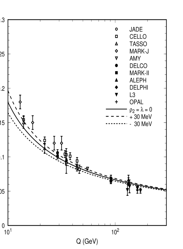
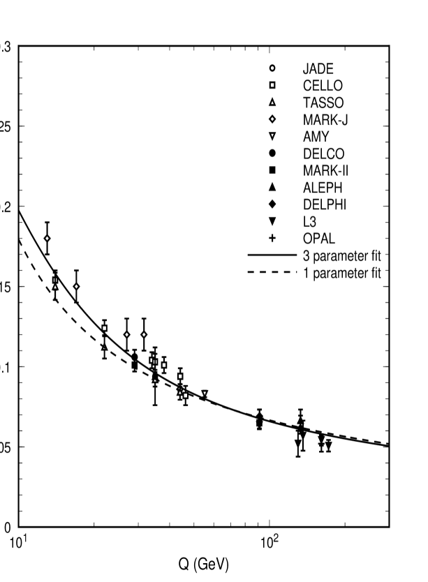
In Fig. 1 we show the fit to the data obtained by setting $\rho_{2}=\lambda=0$. This corresponds to the universal running of the observable given in eq. (9). The fitted value is $\Lambda_{\overline{MS}}^{(5)}=266~{}{\rm MeV}$ with a $\chi^{2}/{\rm d.o.f}=81.7/32$. The dashed lines show the effect of varying $\Lambda_{\overline{MS}}$ by $\pm 30~{}{\rm MeV}$ around the fitted value. We clearly see that the data is falling much too quickly with increasing $Q$ for the asymptotic behaviour to have set in at these scales. The data favours a more steeply falling evolution which could be caused by either higher order corrections with a positive $\rho_{2}$, or power corrections with non-zero $K_{0}$. We therefore perform a 3-parameter fit allowing $\rho_{2}$, $K_{0}$ and $\Lambda_{\overline{MS}}$ to vary independently which is shown in Fig. 2. The minimum $\chi^{2}$ fit is acceptable ($\chi^{2}/{\rm d.o.f}=40.4/30$) and estimating an error by allowing $\chi^{2}$ within $1$ of the minimum gives,

$$\Lambda_{\overline{MS}}^{(5)}=245^{+20}_{-17}~{}{\rm MeV}\qquad{\rm with}\qquad\rho_{2}=-16\mp 11\qquad{\rm and}\qquad\lambda=0.27^{+0.12}_{-0.10}~{}{\rm GeV}.$$

These values of $\rho_{2}$ and $\lambda$ are reasonably small, thereby lending support to our critical assumption that the evolution equation could be parameterized in this way. We can convert the extracted value of $\Lambda_{\overline{MS}}$ into $\alpha_{S}(M_{Z})$ using,

$$\alpha_{s}(M_{Z})=\frac{2\pi}{b\log(Q^{2}/\Lambda_{\overline{MS}}^{2})}\left[1-\frac{2c\log(\log(Q^{2}/\Lambda_{\overline{MS}}^{2}))}{b\log(Q^{2}/\Lambda_{\overline{MS}}^{2})}\right],$$ (14)

and find,

$$\alpha_{S}(M_{Z})=0.1194\pm 0.0014.$$ (15)

The fitted $\rho_{2}$ value may also be converted, if desired, into an estimate of $r_{2}^{\overline{MS}}(\mu=Q)=89\pm 11$. Note that this large value of $r_{2}$ is almost entirely due to the renormalization group predictable $r_{1}^{2}+cr_{1}$ piece relating $\rho_{2}$ and $r_{2}$ (see eq. (7)).

We see that our central value is remarkably close to that obtained by [2]. The main difference is in how the errors are determined. In our approach, the errors are estimated by allowing the uncalculated higher orders to be fitted by the data and the data prefers these to be small. As higher order corrections become known, the new RS-invariant terms, $\rho_{2}$, $\rho_{3}$ etc., can be incorporated and the fit refined.

With such an accurate value of $\alpha_{S}(M_{Z})$, we should expect that applying this approach to other variables should yield consistent results. Unfortunately, the method described here relies on having reliable data over a reasonable range of $Q$ values. Another variable for which a wide range of data has been accumulated is the heavy jet mass, which is obtained by assigning the particles to one of two hemispheres $H_{1}$ and $H_{2}$ according to whether $\vec{p}_{k}\cdot\vec{n}$ is positive or negative, and finding the maximum scaled invariant mass of the hemispheres,

$$\frac{m_{H}^{2}}{s}=\frac{1}{s}\max_{i=1,2}\left(\sum_{k\in H_{i}}p_{k}\right)^{2}.$$ (16)

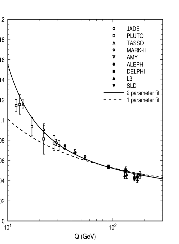
Here $R(Q)=<\!\!m_{H}^{2}/s\!\!>\!\!/1.05$ while $r_{1}=4.52$ [3]. If we repeat the same analysis for this variable, we find that a one parameter fit with $\rho_{2}=\lambda=0$ gives a very poor fit, $\chi^{2}/{\rm d.o.f}=213/29$ and $\Lambda_{\overline{MS}}=368$ MeV. As seen in Fig. 3 the data evolves much faster than the QCD prediction. However, allowing both $\rho_{2}$ and $\lambda$ to vary while using the value of $\Lambda_{\overline{MS}}=245$ MeV obtained from the $<\!\!1-T\!\!>$ analysis gives a much more satisfactory description. Here, $\chi^{2}/{\rm d.o.f}=40.3/27$ while $\rho_{2}=13$ and $\lambda=0.11$ GeV are sufficiently small to support our choice of parameterization.

It is clear that the only certain way to reduce theoretical errors is to compute the NNLO coefficients $\rho_{2}$. However, fitting directly to the energy dependence of the data as we have done enables us to estimate them together with possible power corrections. The renormalization group scale-dependent logarithms are automatically resummed to all orders on integrating eq. (4) and do not add a spurious extra large uncertainty in the extraction of $\Lambda_{\overline{MS}}$ (or equivalently $\alpha_{s}(M_{Z})$). As a result, we have obtained a value of the strong coupling constant that is both competititive with and in agreement with the current world average [11] of a wide range of data,

$$\alpha_{S}(M_{Z})=0.119\pm 0.002.$$

Acknowledgements

We thank Otmar Biebel for clarifying some of the values of the experimental data points used in Ref. [2] and Daniel Wicke for communicating the recent DELPHI measurements the heavy jet mass of Ref. [1]. We also thank Matthew Cullen for helpful comments in the early stages of this work. JMC thanks the UK Particle Physics and Astronomy Research Council for the award of a research studentship.

Figure 1: The average value of $1-T$ obtained experimentally [1, 2] compared with the QCD expectation of eq. (10). The solid line shows the fit to the data with $\rho_{2}=\lambda=0$ corresponding to $\Lambda_{\overline{MS}}=266$ MeV. The long-dashed and short-dashed lines show the effect of altering $\Lambda_{\overline{MS}}$ by $\pm 30$ MeV.

Figure 2: The average value of $1-T$ obtained experimentally [1, 2] compared with the QCD expectation of eq. (10). The dashed line shows the fit to the data with $\rho_{2}=\lambda=0$ while the result of the three parameter fit (to $\Lambda_{\overline{MS}},~{}\rho_{2}$ and $\lambda$) is shown as a solid line.

Figure 3: The average value of the heavy jet mass obtained experimentally [1, 2] compared with the QCD expectation of eq. (10). The dashed line shows the fit to the data with $\rho_{2}=\lambda=0$ while the result of the two parameter fit (to $\rho_{2}$ and $\lambda$) using the value of $\Lambda_{\overline{MS}}$ obtained from the three parameter fit to $<\!\!1-T\!\!>$ is shown as a solid line.

References

-
[1]
MARK-J Collaboration, D.P. Barber et al, Phys. Lett. B85 (1979) 463;
MARK-J Collaboration, D.P. Barber et al, Phys. Rev. Lett. 43 (1979) 901;
PLUTO Collaboration, C. Berger et al, Z. Phys. C12 (1982) 297;
DELCO Collaboration, M. Sakuda et al, Phys. Lett. B152 (1985) 399;
MARK-II Collaboration, A. Peterson et al, Phys. Rev. D37 (1988) 1;
TASSO Collaboration, W. Braunschweig et al, Z. Phys. C41 (1988) 359;
CELLO Collaboration, H. Behrend et al, Z. Phys. C44 (1989) 63;
TASSO Collaboration, W. Braunschweig et al, Z. Phys. C45 (1989) 11;
MARK-II Collaboration, G.S. Abrams et al, Phys. Rev. Lett. 63 (1989) 1558;
AMY Collaboration, Y.K. Li et al, Phys. Rev. D41 (1990) 2675;
TASSO Collaboration, W. Braunschweig et al, Z. Phys. C47 (1990) 187;
OPAL Collaboration, M.Z. Akrawy et al, Z. Phys. C47 (1990) 505;
L3 Collaboration, B. Adeva et al, Z. Phys. C55 (1992) 39;
ALEPH Collaboration, D. Buskulic et al, Z. Phys. C55 (1992) 209;
SLD Collaboration, K. Abe et al, Phys. Rev. D51 (1995) 962;
L3 Collaboration, M. Acciarri et al, Phys. Lett. B371 (1996) 137;
OPAL Collaboration, G. Alexander et al, Z. Phys. C72 (1996) 191;
DELPHI Collaboration, P. Abreu et al, Z. Phys. C73 (1996) 11;
DELPHI Collaboration, P. Abreu et al, Z. Phys. C73 (1997) 229;
ALEPH Collaboration, D. Buskulic et al, Z. Phys. C73 (1997) 409;
L3 Collaboration, M. Acciari et al, Phys. Lett. B404 (1997) 390;
OPAL Collaboration, K. Ackerstaff et al, Z. Phys. C75 (1997) 193;
DELPHI Collaboration, J. Drees et al, DELPHI 97-92 CONF 77;
DELPHI Collaboration, J. Drees et al, 98-18 CONF 119. - [2] P.A. Movilla Fernández et al and the JADE Collaboration, Eur. Phys. J. C1 (1998) 461.
[3]
R.K. Ellis, D.A. Ross and A.E. Terrano,
Nucl. Phys. B178 (1981) 421;
Z. Kunszt, P. Nason, G. Marchesini and B.R. Webber, in Z Physics ar LEP 1, vol. 1, ed. G. Altarelli, R. Kleiss and C. Verzegnassi, CERN Yellow Report 89-08. -
[4]
For reviews and classic references see:
V.I. Zakharov, Nucl. Phys. B385 (1992) 452;
A.H. Mueller, in QCD 20 Years Later, vol. 1 (World Scientific, Singapore, 1993). -
[5]
B.R. Webber, Phys. Lett. B339 (1994) 148;
B.R. Webber, Proc. Summer School on Hadronic Aspects of Collider Physics, Zuoz, Switzerland, 1994 [hep-ph/9411384];
G.P. Korchemsky and G. Sterman, Nucl. Phys. B437 (1995) 415;
G.P. Korchemsky and G. Sterman, Proc. 30th Rencontres de Moriond, Les Arcs, France, 1995 [hep-ph/9505391];
P. Nason and M.H. Seymour, Nucl. Phys. B454 (1995) 291;
R. Akhoury and V.I. Zakharov, Phys. Lett. B357 (1995) 646;
Yu.L. Dokshitzer, G. Marchesini and B.R. Webber, Nucl. Phys. B469 (1996) 93;
R. Akhoury and V.I. Zakharov, Nucl. Phys. B465 (1996) 295;
Yu.L. Dokshitzer and B.R. Webber, Phys. Lett. B404 (1997) 321. - [6] Yu.L. Dokshitzer and B.R. Webber, Phys. Lett. B352 (1995) 451.
[7]
G. Grunberg, Phys. Lett. B95 (1980) 70;
G. Grunberg, Phys. Rev. D29 (1984) 2315. - [8] A. Dhar and V. Gupta, Phys. Rev. D29 (1984) 2822.
- [9] D.T. Barclay, C.J. Maxwell and M.T. Reader, Phys. Rev. D49 (1994) 3480.
- [10] C.J. Maxwell, Phys. Lett. B409 (1997) 450.
- [11] R.M. Barnett et al, Phys. Rev. D54 (1996) 1 and 1997 off-year partial update from http://pdg.lbl.gov.