Local duality and nonleptonic $B$ decay

Abstract

In the large $N_{c}$ limit, the nonleptonic width of the $B$ meson is determined by the lepton mass spectrum in semileptonic $B$ decay and the hadron mass spectrum in $\tau$ decay. This result can be compared with the nonleptonic width computed using the operator product expansion and local duality, to estimate the violation of local duality in $B$ decay. In the absence of the required data, we use experimental Monte Carlo predictions and find that the difference is small, at the few percent level. We estimate the theoretical uncertainty in our results from higher order corrections (including $1/N_{c}$ effects). We also identify a new contribution to the $\Lambda_{b}-B$ lifetime difference.

I Introduction

Inclusive decays for heavy-quark hadrons such as $B$ mesons are computed in a systematic expansion in inverse powers of the heavy quark mass using the operator product expansion (OPE). Decay rates are related to the discontinuity of scattering amplitudes at physical cuts, so the calculation is necessarily performed for time-like momentum transfer and is not a short-distance process for which the OPE is valid. Nevertheless, one can still use the OPE for suitably averaged quantities. The simplest example is $R(s)$, the inclusive rate for $e^{+}e^{-}\to{\rm hadrons}$, which is related to the discontinuity in the vacuum polarization amplitude $\Pi(s)$ along the real axis for $s>0$. The operator product expansion can be applied to $\Pi(s)$ far away from the physical cuts, such as at complex $s=s_{0}+i\Delta$, $\Delta\gg\Lambda_{\rm QCD}$, to give $\Pi(s)$ as an expansion in $\Lambda_{\rm QCD}^{2}/s$ and $\alpha_{s}$. Analyticity can then be used to relate $\Pi(s_{0}+i\Delta)$ to an integral of the form [1]

$$\int_{0}^{\infty}{R(s)\over(s-s_{0})^{2}+\Delta^{2}}\,{\rm d}s\,.$$ (1)

Thus smeared averages of $R(s)$ can be computed using perturbation theory. The $\alpha_{s}$ corrections to these depend on the smearing width $\Delta$, and are not under control as $\Delta\to 0$. In practice $\Delta$ is made as small as possible while keeping the radiative corrections under control. Typically $\Delta$ is chosen to be $\Delta\gtrsim 500\,$MeV. One expects that perturbative computations agree with data, provided one averages over a large number of hadronic resonances.

A similar situation exists in inclusive semileptonic $B$ decays, $B\to X_{c}\,e\,\bar{\nu}$ [3, 4]. The differential decay distribution ${\rm d}\Gamma^{(B,{\rm sl})}/{\rm d}q^{2}{\rm d}E_{e}{\rm d}E_{\nu}$ can be computed using the operator product expansion [5, 6, 7, 8]. Here $q^{2}$ is the invariant mass of the lepton pair, and $E_{e}$ and $E_{\nu}$ are the energy of the electron and neutrino, respectively. The total semileptonic decay rate $\Gamma^{(B,{\rm sl})}$ automatically involves averaging over different hadronic states, and one expects that the OPE computation for $\Gamma^{(B,{\rm sl})}$ is valid. Inclusive nonleptonic $B\to X_{c}$ decays can also be computed using an OPE [4, 9]. In this case, there is no variable such as $q^{2}$ to integrate over, so the computation has no intrinsic smearing. One must then make the assumption of local duality, that the quark and hadron computations agree at a single kinematic point. In the case of $R(s)$, this would mean that one could compute $R(s)$ for each value of $s$. This is clearly false when there are narrow resonances (e.g., in the $\Upsilon$ region), but is valid elsewhere because the large number of overlapping hadronic resonances provide a natural smearing mechanism. An important question is the extent to which local duality holds for nonleptonic $B$ meson decays. There is a long-standing claimed discrepancy between theory and experiment in the $B$ meson semileptonic branching ratio and in the $\Lambda_{b}$ to $B$ lifetime ratio, and the failure of local duality is one way to resolve these.

In this paper, we study the violation of local duality using the $1/N_{c}$ expansion of QCD [10]. In this limit, we show that the nonleptonic $B$ meson decay rate $\Gamma^{(B,{\rm nl})}$ can be expressed in terms of the product of ${\rm d}\Gamma^{(B,{\rm sl})}/{\rm d}q^{2}$, the invariant mass distribution of the lepton pair in semileptonic $B$ decay, and ${\rm d}\Gamma^{(\tau,{\rm h})}/{\rm d}q^{2}$, the hadron mass distribution in nonleptonic $\tau$ decay. One gets a quantitative measure of the violation of local duality in the large $N_{c}$ limit by comparing the prediction for $\Gamma^{(B,{\rm nl})}$ using the OPE with that using the experimental data for ${\rm d}\Gamma^{(B,{\rm sl})}/{\rm d}q^{2}$ and ${\rm d}\Gamma^{(\tau,{\rm h})}/{\rm d}q^{2}$, and a large $N_{c}$ factorization formula derived here. We estimate the accuracy to which the large $N_{c}$ results should be valid in QCD.

II Basic definitions and results

Nonleptonic $B$ meson decays are dominantly due to the weak Hamiltonian

$$H={4G_{F}\over\sqrt{2}}\,a^{(B,{\rm nl})}\,V_{cb}V_{uq}^{*}\,\Big{[}c_{1}(m_{b})\,(\bar{c}\,\gamma_{\mu}P_{L}\,b)\,(\bar{q}\,\gamma^{\mu}P_{L}\,u)+c_{2}(m_{b})\,(\bar{q}\,\gamma_{\mu}P_{L}\,b)\,(\bar{c}\,\gamma^{\mu}P_{L}\,u)\Big{]}\,,$$ (2)

where $P_{L}=(1-\gamma_{5})/2$ and $q=d,s$. The Hamiltonian in Eq. (2) is renormalized at the scale $\mu=m_{b}$. The coefficient $a^{(B,{\rm nl})}=1+(2{\alpha_{\rm em}/3\pi})\ln({M_{W}/m_{b}})$ is the electromagnetic correction. The coefficients $c_{i}$ are QCD corrections given by $c_{1,2}=(c_{+}\pm c_{-})/2$, where

$$c_{+}(\mu)=\left[{\alpha_{s}(\mu)\over\alpha_{s}(M_{W})}\right]^{-6/23},\qquad c_{-}(\mu)=\left[{\alpha_{s}(\mu)\over\alpha_{s}(M_{W})}\right]^{12/23},$$ (3)

at one loop order. At next-to-leading order [11], $c_{1}(m_{b})=1.13$ and $c_{2}(m_{b})=-0.29$ for $\alpha_{s}(M_{Z})=0.118$. The $c_{1}$ and $c_{2}$ terms are effective charged and neutral current interactions, respectively.

Nonleptonic $B$ decay widths are computed by taking the decay amplitude $\langle X_{c}|H|B\rangle$, squaring, and summing over all possible final states. A simpler method is to compute the imaginary part of the $B\to B$ forward scattering amplitude with an insertion of $H$ and $H^{\dagger}$. Diagrams involving spectator quarks [12, 13], such as Pauli interference, weak annihilation, and $W$-exchange are of order $\Lambda_{\rm QCD}^{3}/m_{b}^{3}$ relative to free quark decay (since they depend on matrix elements of four-quark operators), and can be neglected for the purposes of this paper. In the large $N_{c}$ limit, annihilation effects are enhanced by a factor $N_{c}$ relative to free quark decay. While this means that annihilation diagrams are formally dominant at $N_{c}=\infty$, they can still be neglected for $N_{c}=3$ because the $N_{c}$ enhancement does not compensate for the $1/m_{b}^{5}$ suppression factor, since the diagram is helicity suppressed and involves four-quark operators.

The free quark decay diagram in Fig. 1 is redrawn in Fig. 2 to show the color flows. The charged and neutral current terms in the weak Hamiltonian in Eq. (2) are denoted by the exchange of color singlet charged and neutral “gauge bosons.” This is a convenient way of showing the color flows in the diagrams. The order in $N_{c}$ of the various graphs can be computed by using a factor of $N_{c}$ for each closed color loop, and $1/\sqrt{N_{c}}$ for each external meson. In the large $N_{c}$ limit, Fig. 2(a) and (b) are ${\mathcal{O}}\left(N_{c}\right)$, and (c) is ${\mathcal{O}}\left(1\right)$. Fig. 2(a), (b) and (c) will be referred to as the charged current, neutral current, and interference diagrams, respectively. In the large $N_{c}$ limit, arbitrary planar gluons must be summed over, which is represented schematically by the shaded regions in the figures. The leading diagrams have arbitrary planar exchanges within each quark loop, but exchanges between the two quark loops are suppressed by at least two powers of $N_{c}$. Thus in the large $N_{c}$ limit, Fig. 2(a) and (b) factorize into the product of two non-perturbative matrix elements. They are: (i) The matrix element of two currents in a $B$ meson; (ii) The matrix element of two currents in the vacuum. These will be related to inclusive semileptonic $B$ decay and hadronic $\tau$ decay, respectively.

Consider the inclusive decay of an initial particle $I$ with velocity $v$ due to the Hamiltonian

$$H={4G_{F}\over\sqrt{2}}\,J^{\mu}j_{\mu}\,.$$ (4)

The decaying particle $I$ and the weak currents $J^{\mu}$ and $j^{\mu}$ will be different for the three cases we need in this paper—nonleptonic $B$ decay, semileptonic $B$ decay, and hadronic $\tau$ decay. In these decays, the weak Hamiltonian has factors in addition to those shown explicitly in Eq. (4), such as CKM angles or renormalization group coefficients, which will be included later.

Define the tensors

$$W^{\mu\nu}(v,q)=(2\pi)^{3}\,\sum_{X}\delta^{4}(m_{I}\,v-q-p_{X})\,\langle I(v)|J^{\mu\dagger}|X\rangle\,\langle X|J^{\nu}|I(v)\rangle\,,$$ (5)

and

$$\Omega^{\mu\nu}(q)=(2\pi)^{4}\,\sum_{Y}\delta^{4}(q-p_{Y})\,\langle 0|j^{\mu\dagger}|Y\rangle\,\langle Y|j^{\nu}|0\rangle\,.$$ (6)

In terms of $W$ and $\Omega$, the weak decay rate is given by

$${{\rm d}\Gamma\over{\rm d}q^{2}\,{\rm d}q_{0}}={2G_{F}^{2}\over\pi^{2}}\sqrt{q_{0}^{2}-q^{2}}\,W^{\mu\nu}(v,q)\,\Omega_{\mu\nu}(q)\,,$$ (7)

as long as the diagrams for the process factorize, e.g., as in Fig. 2(a) or (b). This is the factorization formula which we will use in the rest of the paper.

The hadronic tensor $W^{\mu\nu}$ is identical to the one that appears in the OPE for semileptonic decays [6, 7]. It can be expanded as

$$W^{\mu\nu}=-g^{\mu\nu}W_{1}+v^{\mu}v^{\nu}W_{2}-i\varepsilon^{\mu\nu\alpha\beta}v_{\alpha}q_{\beta}W_{3}+q^{\mu}q^{\nu}W_{4}+(q^{\mu}v^{\nu}+q^{\nu}v^{\mu})W_{5}\,,$$ (8)

where $W_{i}$ are functions of $q^{2}$ and $q\cdot v$. $\Omega^{\mu\nu}$ can be decomposed into transverse and longitudinal parts

$$\Omega^{\mu\nu}=(-q^{2}g^{\mu\nu}+q^{\mu}q^{\nu})\,\Omega_{T}+q^{\mu}q^{\nu}\,\Omega_{L}\,,$$ (9)

where $\Omega_{T,L}$ are functions of $q^{2}$. Contracting Eqs. (8) and (9) gives

$$W^{\mu\nu}\,\Omega_{\mu\nu} = \Omega_{T}\left[3q^{2}\,W_{1}-q^{2}\,W_{2}+(q\cdot v)^{2}\,W_{2}\right]$$ (10)

$$+ \Omega_{L}\left[-q^{2}\,W_{1}+(q\cdot v)^{2}\,W_{2}+q^{4}\,W_{4}+2q^{2}(q\cdot v)\,W_{5}\right].$$ (11)

Both $W^{\mu\nu}$ and $\Omega_{\mu\nu}$ are calculable in an operator product expansion. They are related to the discontinuities across the cut of the amplitudes $T^{\mu\nu}$ and $\Pi_{\mu\nu}$ defined by

$$T^{\mu\nu} = -i\int{\rm d}^{4}x\,e^{-iq\cdot x}\,\langle B(v)|\,T\{J^{\mu\dagger}(x)\,J^{\nu}(0)\}|B(v)\rangle\,,$$ (12)

$$\Pi^{\mu\nu} = -i\int{\rm d}^{4}x\,e^{-iq\cdot x}\,\langle 0|\,T\{j^{\mu\dagger}(x)\,j^{\nu}(0)\}|0\rangle\,,$$ (13)

i.e., $W^{\mu\nu}={\rm Im}\,T^{\mu\nu}/\pi$ and $\Omega^{\mu\nu}=2\,{\rm Im}\,\Pi^{\mu\nu}$. $T^{\mu\nu}$ and $\Pi^{\mu\nu}$ have a form factor decomposition similar to $W^{\mu\nu}$ and $\Omega^{\mu\nu}$ in Eqs. (8) and (9), with $W_{i}\to T_{i}$ and $\Omega_{i}\to\Pi_{i}$. In the complex $q^{2}$ plane, $\Pi^{\mu\nu}$ has a cut along the real axis for $q^{2}\gtrsim 0$. $T^{\mu\nu}$ has two cuts along the real axis for $q^{2}\lesssim(m_{b}-m_{c})^{2}$ corresponding to intermediate states with a charm quark, and for $q^{2}\gtrsim(m_{b}+2m_{c})^{2}$ corresponding to intermediate states with a $\bar{c}$ and two $b$ quarks.

A Inclusive hadronic $\tau$ decay

The weak Hamiltonian at $\mu=m_{\tau}$ for hadronic $\tau$ decay $\tau\to\nu_{\tau}\,X$ is

$$H={4G_{F}\over\sqrt{2}}\,a^{(\tau)}\,V_{uq}^{*}\,(\bar{\nu}_{\tau}\,\gamma_{\mu}P_{L}\,\tau)\,(\bar{q}\,\gamma^{\mu}P_{L}\,u).$$ (14)

$a^{(\tau)}=1+(\alpha_{\rm em}/\pi)\ln(M_{W}/m_{\tau})$ is the electromagnetic correction. There are no QCD corrections to Eq. (14) since the quark part is a conserved current.

The hadronic $\tau$ decay amplitude clearly factors into hadronic and leptonic parts, irrespective of whether $N_{c}$ is large or not, since no gluons can be exchanged between the quark and lepton parts of the diagram. The leptonic part of the diagram is calculable, and gives

$$\begin{array}[]{ll}W^{(\tau)}_{1}=\frac{1}{2}\,(m_{\tau}-q_{0})\,\delta(\Delta)\,,&W^{(\tau)}_{2}=m_{\tau}\,\delta(\Delta)\,,\\ W^{(\tau)}_{3}=-W^{(\tau)}_{5}=\frac{1}{2}\,\delta(\Delta)\,,&W^{(\tau)}_{4}=0\,,\end{array}$$ (15)

where $\Delta=m_{\tau}^{2}+q^{2}-2m_{\tau}q_{0}$. The hadronic part of the $\tau$ decay diagram is precisely $\Omega$ for the charged current nonleptonic $B$ decay diagram. The factorization formula Eq. (7) can be applied to this case, with $W_{\mu\nu}$ set equal to $W^{(\tau)}_{\mu\nu}$. $\Omega$ in $\tau$ decay is defined to be $\Omega^{(\tau)}_{T,L}$, the sum of $\Omega$’s for the weak currents $V_{ud}(\bar{d}\,\gamma_{\mu}P_{L}\,u)$ and $V_{us}(\bar{s}\,\gamma_{\mu}P_{L}\,u)$, so that the CKM angle is included in $\Omega^{(\tau)}$. Integrating over ${\rm d}q_{0}$ using $\delta(\Delta)$, gives [14]

$${{\rm d}\Gamma^{(\tau,{\rm h})}\over{\rm d}q^{2}}={G_{F}^{2}\over 8\pi^{2}\,m_{\tau}^{3}}\left|a^{(\tau)}\right|^{2}(m_{\tau}^{2}-q^{2})^{2}\left[(m_{\tau}^{2}+2q^{2})\,\Omega^{(\tau)}_{T}+m_{\tau}^{2}\,\Omega^{(\tau)}_{L}\right],$$ (16)

where $q^{2}$ is the invariant mass-squared of the hadrons in the final state.

B Inclusive semileptonic $B$ decay

Inclusive semileptonic $B\to X_{c}\,e\,\bar{\nu}$ decay is due to the weak Hamiltonian

$$H={4G_{F}\over\sqrt{2}}\,a^{(B,{\rm sl})}\,V_{cb}\,(\bar{c}\,\gamma_{\mu}P_{L}\,b)\,(\bar{e}\,\gamma^{\mu}P_{L}\,\nu).$$ (17)

$a^{(B,{\rm sl})}=1+(\alpha_{\rm em}/\pi)\ln(M_{W}/m_{b})$ is the electromagnetic correction. There are no QCD corrections since the quark part of the Hamiltonian is a conserved current. As for hadronic $\tau$ decay, the semileptonic $B$ decay diagram factorizes into a hadronic and leptonic part, irrespective of whether $N_{c}$ is large or not. The leptonic part $\Omega^{\mu\nu}$ is calculable,

$$\Omega^{(B,{\rm sl})}_{T} = {1\over 12\pi}\,{(q^{2}-m_{e}^{2})^{2}\,(2q^{2}+m_{e}^{2})\over 2q^{6}}\,,$$ (18)

$$\Omega^{(B,{\rm sl})}_{L} = {1\over 8\pi}\,{(q^{2}-m_{e}^{2})^{2}\,m_{e}^{2}\over q^{6}}\,,$$ (19)

where $q^{2}$ is the invariant mass-squared of the lepton pair. Therefore, ${\rm d}\Gamma^{(B,{\rm sl})}/{\rm d}q^{2}{\rm d}q_{0}$ gives information on the hadronic part $W^{(B,{\rm sl})}_{\mu\nu}$. Using differential $B$ decay spectra for $e$, $\mu$, and $\tau$, it is possible to measure $W^{(B,{\rm sl})}_{1,\ldots,5}$ [15]. This seems to be a remote possibility, so in the rest of this paper we neglect lepton masses. In the $m_{e}\to 0$ limit, Eqs. (7) and (8) give

$${{\rm d}\Gamma^{(B,{\rm sl})}\over{\rm d}q^{2}\,{\rm d}q_{0}}={2G_{F}^{2}\over\pi^{2}}\left|a^{(B,{\rm sl})}\right|^{2}\sqrt{q_{0}^{2}-q^{2}}\left[3q^{2}\,W^{(B,{\rm sl})}_{1}+(q_{0}^{2}-q^{2})\,W^{(B,{\rm sl})}_{2}\right]{1\over 12\pi}\,,$$ (20)

where the CKM angle $\left|V_{cb}\right|^{2}$ has been absorbed into the definition of $W^{(B,{\rm sl})}_{1,2}$.

C The OPE calculation for nonleptonic $B$ decay

The nonleptonic $B$ decay rate can be computed using perturbation theory if one assumes local duality. To order $\Lambda_{\rm QCD}^{2}/m_{b}^{2}$, the result is [9]

$$\Gamma^{(B,{\rm nl})}[b\to c\bar{u}(d+s)]=3\Gamma_{0}\left|a^{(B,{\rm nl})}\right|^{2} {}\bigg{\{}{c_{-}^{2}+2c_{+}^{2}\over 3}\,\bigg{[}\bigg{(}1+{\lambda_{1}\over 2m_{b}^{2}}\bigg{)}+{3\lambda_{2}\over m_{b}^{2}}\bigg{(}\rho\,{{\rm d}\over{\rm d}\rho}-2\bigg{)}\bigg{]}f(\rho)$$ (22)

$${}+4(c_{-}^{2}-c_{+}^{2})\,{\lambda_{2}\over m_{b}^{2}}\,(1-\rho)^{3}\bigg{\}}+\ldots\,,$$

$$\Gamma^{(B,{\rm nl})}[b\to c\bar{c}(d+s)]=3\Gamma_{0}\left|a^{(B,{\rm nl})}\right|^{2} {}\bigg{\{}{c_{-}^{2}+2c_{+}^{2}\over 3}\,\bigg{[}\bigg{(}1+{\lambda_{1}\over 2m_{b}^{2}}\bigg{)}+{3\lambda_{2}\over m_{b}^{2}}\bigg{(}\rho\,{{\rm d}\over{\rm d}\rho}-2\bigg{)}\bigg{]}g(\rho)$$ (24)

$${}+4(c_{-}^{2}-c_{+}^{2})\,{\lambda_{2}\over m_{b}^{2}}\,h(\rho)\bigg{\}}+\ldots\,,$$

where $\rho=m_{c}^{2}/m_{b}^{2}$, $\Gamma_{0}=G_{F}^{2}m_{b}^{5}|V_{cb}|^{2}/(192\pi^{3})$, and

$$f(\rho) = 1-8\rho+8\rho^{3}-\rho^{4}-12\rho^{2}\ln\rho\,,$$ (25)

$$g(\rho) = \sqrt{1-4\rho}\,(1-14\rho-2\rho^{2}-12\rho^{3})+24\rho^{2}(1-\rho^{2})\ln{1+\sqrt{1-4\rho}\over 1-\sqrt{1-4\rho}}\,,$$ (26)

$$h(\rho) = \sqrt{1-4\rho}\,(1+\rho/2+3\rho^{2})-3\rho(1-2\rho^{2})\ln{1+\sqrt{1-4\rho}\over 1-\sqrt{1-4\rho}}\,.$$ (27)

The ellipses in Eqs. (22) and (24) denote corrections of order $\Lambda_{\rm QCD}^{3}/m_{b}^{3}$ and $\alpha_{s}(m_{b})$. The total nonleptonic decay rate is the sum of Eq. (22) and Eq. (24). $\alpha_{s}$ corrections will be included when we use these results in the next section.

III A (not so) toy model: $c_{2}=0$

The total nonleptonic decay rate depends on the short distance QCD corrections $c_{1}$ and $c_{2}$. The validity of local duality depends on long distance effects, such as the masses and widths of hadronic resonances. One can test local duality in the nonleptonic $B$ decay rate by studying a hypothetical world in which $c_{2}=0$ and $c\bar{c}(d+s)$ final states are turned off. This tests local duality only for the charged current part of Eq. (2).

The charged current diagram Fig. 2(a) factorizes in the large $N_{c}$ limit, so Eq. (7) can be used. Combining this with Eqs. (11), (16), and (20), one finds

$${{\rm d}\Gamma^{(B,{\rm nl})}\over{\rm d}q^{2}} = \left|{a^{(B,{\rm nl})}\over a^{(B,{\rm sl})}a^{(\tau)}}\right|^{2}{{\rm d}\Gamma^{(B,{\rm sl})}\over{\rm d}q^{2}}\,{{\Omega^{(\tau)}_{T}}(q^{2})\over{\Omega^{(B,{\rm sl})}_{T}}(q^{2})},$$ (28)

$${{\Omega^{(\tau)}_{T}}(q^{2})\over{\Omega^{(B,{\rm sl})}_{T}}(q^{2})} = {{\rm d}\Gamma^{(\tau,{\rm h})}\over{\rm d}q^{2}}\,{96\pi^{3}m_{\tau}^{3}\over G_{F}^{2}}\,{1\over(m_{\tau}^{2}-q^{2})^{2}\,(m_{\tau}^{2}+2q^{2})}\,.$$ (29)

$\Omega_{L}$ has been neglected in this equation because it is proportional to the current quark masses of the $u$, $d$ and $s$ quarks. In the large $N_{c}$ limit, one can compute the nonleptonic $B$ decay rate in terms of the semileptonic $B$ decay rate and the $\tau$ hadronic decay rate. This is the main result in this paper.

Equation (28) will be used to test local duality in nonleptonic $B$ decay. Assuming that the OPE computation of the total semileptonic decay rate is valid, one knows that the integral of the experimentally measured spectrum ${\rm d}\Gamma^{(B,{\rm sl})}/{\rm d}q^{2}$ over $q^{2}$ is equal to the OPE value of the total decay rate. Moments of the measured $q^{2}$ spectrum and of the OPE prediction should also agree; however, the higher order $\alpha_{s}$ and $1/m$ corrections get larger for higher moments. As a result, the integral of the $q^{2}$ spectra from experiment and from the OPE should agree when weighted with a sufficiently smooth and broad function, but not necessarily point by point. A similar result holds for the $q^{2}$ spectrum in $\tau$ hadronic decay. In Eq. (28) above, the experimentally measured $q^{2}$ spectrum in semileptonic $B$ decay is multiplied by the experimentally measured $q^{2}$ spectrum in hadronic $\tau$ decay. The $\tau$ decay spectrum is not a smooth function (see Fig. 3), which is what makes the test non-trivial.

A Error estimates

The test of local duality is to compare $\Gamma^{(B,{\rm nl})}$ in Eq. (22) calculated using the OPE and perturbation theory with $\Gamma^{(B,{\rm nl})}$ in Eq. (28) obtained from experimental data. Before we discuss the result, it is worth examining the errors in the formulæ we have derived. The leading corrections to Eq. (28) are factorization violating diagrams involving two-gluon exchange between the two quark loops in Fig. 2(a). Single gluon exchange is forbidden by color conservation. If both gluons are hard, the diagram can be computed in perturbation theory. It is order $\alpha_{s}^{2}$, but is not part of the BLM series[16] $(\alpha_{s}/\pi)^{r+1}\beta_{0}^{r}$, where $\beta_{0}=11-2n_{f}/3$ is the coefficient of the one-loop QCD $\beta$-function. If both gluons are soft, the correction is of order $\Lambda_{\rm QCD}^{4}/m_{b}^{4}$, and if one gluon is hard and one is soft, the correction is of order $\alpha_{s}\Lambda_{\rm QCD}^{2}/m_{b}^{2}$. The leading power suppressed corrections to Eq. (28) are of order $\alpha_{s}\Lambda_{\rm QCD}^{2}/m_{b}^{2}$ or $\Lambda_{\rm QCD}^{3}/m_{b}^{3}$. The $\Lambda_{\rm QCD}^{2}/m_{b}^{2}$ corrections cancel between $\Gamma^{(B,{\rm nl})}$ and $\Gamma^{(B,{\rm sl})}$. The first correction in the OPE for $\Pi_{\mu\nu}$ is order $\Lambda_{\rm QCD}^{4}/q^{4}$. Both $\tau$ decay and $B$ decay involve summing over $\bar{d}u$ and $\bar{s}u$ final states with weights $\left|V_{ud}\right|^{2}$ and $\left|V_{us}\right|^{2}$, respectively, so both contributions are correctly included in Eq. (28) when one uses the measured $\tau$ hadronic decay rate. In a world with $c_{2}=0$, the largest correction to Eq. (28) is the Pauli interference contribution, of order $(16\pi^{2}/N_{c})f_{B}^{2}/m_{B}^{2}\sim 5\%$. Very little use has been made of the $1/N_{c}$ expansion in the theoretical analysis for $c_{2}=0$. However, the skeptic might argue that the error estimate is based on the OPE, which is what is being tested in the first place. The factorization violation contributions to the decay rate are $1/N_{c}^{2}$ corrections. This gives an OPE-independent error estimate of $\sim 10\%$.

B Data analysis

The hadronic $\tau$ decay spectrum (i.e., $\Omega^{(\tau)}$) is only measured in the region $q^{2}<m_{\tau}^{2}$. In the region $\Delta^{2}<q^{2}<m_{B}^{2}$, (with $\Delta^{2}<m_{\tau}^{2}$), we use the perturbative calculation [14], including corrections to $\Omega^{(\tau)}(q^{2})$ up to order $\alpha_{s}^{2}$ with $\alpha_{s}(m_{\tau})=0.32$. Higher order terms are negligible for our purposes. We vary $\Delta^{2}$ between $2-3\,{\rm GeV}^{2}$ and check that our conclusions are unaffected by the precise value of $\Delta$. The region $q^{2}<m_{\tau}^{2}$ is where the largest violations of local duality are expected in $\Omega$, and experimental data suggests that local duality already holds at some level for $q^{2}\gtrsim 1.5\,{\rm GeV}^{2}$. For $W_{\mu\nu}$ the largest deviations from local duality are expected near $q^{2}_{\rm max}\simeq(m_{b}-m_{c})^{2}$.

For the hadron invariant mass spectrum in $\tau$ decay we use a Monte Carlo distribution that has been tuned to be consistent with CLEO data. This can be used to determine $\Omega^{(\tau)}_{T}(q^{2})$. In Fig. 3 we have plotted $\Omega^{(\tau)}_{T}(q^{2})/\Omega^{(B,{\rm sl})}_{T}(q^{2})$ together with the perturbation theory prediction for this ratio (including corrections up to order $\alpha_{s}^{2}$). The lepton invariant mass spectrum in semileptonic $B$ decay has not yet been measured, so we use the CLEO Monte Carlo. The normalized mass spectrum is plotted in Fig. 4 as a function of $q^{2}$ together with the prediction of perturbation theory. The shape of this curve is rather insensitive to the order $\alpha_{s}$ and $\alpha_{s}^{2}\beta_{0}$ corrections[18].

It is simplest to normalize the nonleptonic rate to the semileptonic rate. This eliminates the order $\Lambda_{\rm QCD}^{2}/m_{b}^{2}$ corrections and reduces the perturbative corrections as well. The result for the $B$ meson decay rate using the factorization formula Eq. (28) and the CLEO Monte Carlo spectra is

$$\Gamma^{(B,{\rm nl})}[b\to c\bar{u}(d+s)]/\Gamma^{(B,{\rm sl})}\bigg{|}_{\rm CLEO}=3.32\left|c_{1}\right|^{2}.$$ (30)

The result for the OPE calculation at this order is

$${{\rm d}\Gamma^{(B,{\rm nl})}[b\to c\bar{u}(d+s)]/{\rm d}q^{2}\over{\rm d}\Gamma^{(B,{\rm sl})}/{\rm d}q^{2}}=3\left|c_{1}\,a^{(B,{\rm nl})}\over a^{(B,{\rm sl})}\right|^{2}\left[1+{\alpha_{s}(q^{2})\over\pi}+0.173\beta_{0}\left({\alpha_{s}(q^{2})\over\pi}\right)^{2}+\ldots\right]\,.$$ (31)

Expressing $\alpha_{s}(q^{2})$ in terms of $\alpha_{s}(m_{b})=0.22$ and neglecting nonperturbative and higher order perturbative corrections, this implies $\Gamma^{(B,{\rm nl})}[b\to c\bar{u}(d+s)]/\Gamma^{(B,{\rm sl})}=3\left|c_{1}a^{(B,{\rm nl})}/a^{(B,{\rm sl})}\right|^{2}\left(1+0.07+0.025\right)=3.21\left|c_{1}\right|^{2}$. The difference is surprisingly small, at the 3% level, which is less than the 5% theoretical uncertainty of the calculation. So we conclude that the uncertainties in the charged current contribution to $b$ hadron lifetimes due to local duality violation are unlikely to exceed the $\sim 5\%$ percent level. Of course, it is very important to repeat this analysis using real data for the lepton mass spectrum in semileptonic $B$ decay, ${\rm d}\Gamma^{(B,{\rm sl})}/{\rm d}q^{2}$, especially since the Monte Carlo predictions used above (solid curve in Fig. 4) differ significantly from perturbation theory in the low $q^{2}$ region.

IV Reality

In the real world with $c_{2}\neq 0$, there are several effects that restrict our calculational ability. The interference term Fig. 2(c), is a $1/N_{c}$ correction and does not factorize. Its contribution is order $(2/N_{c})|c_{2}/c_{1}|\sim 18\%$ of the $B\to c\bar{u}(d+s)$ decay rate. It has been argued that deviations from local duality are likely to be larger for this contribution[19].

The neutral current decay Fig. 2(b) also factorizes. $W_{\mu\nu}$ for this decay can be determined from semileptonic $B$ decay due to the (hypothetical) neutral current $\bar{d}\gamma^{\mu}P_{L}b$. This can be related to semileptonic $B$ decay due to the weak current $\bar{u}\gamma^{\mu}P_{L}b$ by isospin invariance. $\Omega_{\mu\nu}$ for the neutral current decay is the vacuum polarization contribution due to the $\bar{c}\gamma^{\mu}P_{L}u$ current, for which there is no experimental information. The neutral current contribution to the decay width is order $|c_{2}/c_{1}|^{2}\sim 7\%$.

We have neglected $b\to c\bar{c}(s+d)$ decays. These can also be factorized in the large $N_{c}$ limit. The vacuum polarization $\Omega$ is due to $\bar{s}\gamma^{\mu}P_{L}c$ and $\bar{d}\gamma^{\mu}P_{L}c$ currents, for which there is no experimental information. Thus our calculational method, while valid in principle, is not useful for $b\to c\bar{c}(s+d)$. Experimentally, one can separate the $b\to c\bar{u}(s+d)$ and $b\to c\bar{c}(s+d)$ contributions to the nonleptonic decay rate by counting the number of charm quarks in the final state, and the results of the previous section can be used for the $b\to c\bar{u}(s+d)$ part.

V Conclusions

We have estimated the violation of local duality for nonleptonic $B$ decay with $c_{2}=0$ to be less than the theoretical uncertainty in our calculation of $\sim 5\%$. It is important to redo the analysis using experimental data, rather than Monte Carlo, once it is available. One can also view the results in a different way: the factorization formula allows one to compute the nonleptonic $B$ decay rate using the lepton mass spectrum in semileptonic $B$ decay and the hadron mass spectrum in $\tau$ decay without using an OPE. In the world $c_{2}=0$, one can predict this rate with an accuracy of 5%. In the real world, one can compute the $b\to c\bar{u}(s+d)$ part of the decay rate with approximately 20% accuracy. The results cannot easily be extended to $D$ meson decays, because the $\Lambda_{\rm QCD}^{3}/m_{c}^{3}$ corrections in the charm sector are $\sim 100\%$ of the charm quark decay result.

These reasonably tight limits on local duality violation do not resolve the question of the $\Lambda_{b}$ to $B$ lifetime ratio. Of course, duality violation in $b\to c\bar{c}(d+s)$ and in the $c_{1}c_{2}$ interference contributions are probably larger. While enhancing the average number of charm in $B$ decay seems experimentally disfavored, the $c_{1}c_{2}$ interference remains suspect. It is also possible that spectator effects are anomalously large in $\Lambda_{b}$ decay—in fact, there are six-quark operators (see Fig. 5) which contribute roughly of order $(16\pi^{2})^{2}(f_{B}/m_{b})^{4}/N_{c}$ relative to the $b$ quark decay. These have not been analyzed, and may significantly affect the spectator contribution to $\Lambda_{b}$ decay. They do not occur for $B$ meson decay, and so contribute to the $\Lambda_{b}-B$ lifetime difference.

In semileptonic $B$ decay, there is no $1/m_{b}$ correction [3]. This is also true in nonleptonic $B$ decays, if one uses the OPE [4]. In other processes which do not have an OPE, it is known that one can get arbitrary power suppressed corrections [20]. It has been suggested that there might be $1/m_{b}$ corrections in inclusive nonleptonic decay rates [21]. In the large $N_{c}$ limit with $c_{2}=0$, Eq. (28) shows that the $1/m_{b}$ corrections to the nonleptonic decay rate can be computed in terms of the corrections to the lepton mass spectrum in semileptonic $B$ decay and the hadron mass spectrum in $\tau$ decay. At least one of these would have to have a $1/m_{b}$ correction if there is one in the nonleptonic decay rate.

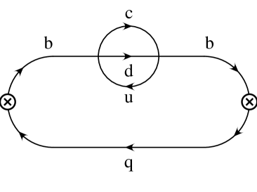
FIG. 1.: Leading contribution to $B$ meson decay ($B\to B$ forward scattering amplitude). The weak currents have been contracted to a point, and $\otimes$ represent quark bilinears that create or annihilate $B$ mesons.

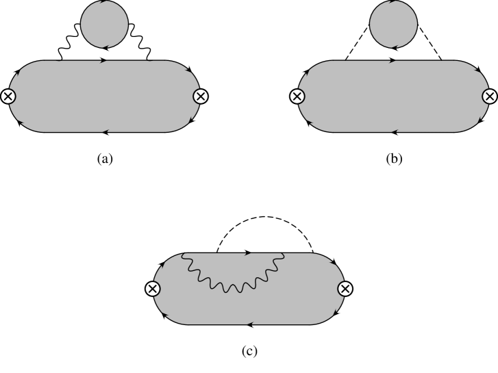
FIG. 2.: Free quark decay diagrams showing the color flow. The charged and neutral current interactions in Eq. (2) are represented by the exchange of gauge bosons denoted by wiggly and dashed lines, respectively. The shaded regions represent arbitrary planar gluons.

FIG. 3.: $\Omega^{(\tau)}_{T}(q^{2})/\Omega^{(B,{\rm sl})}_{T}(q^{2})$ from Monte Carlo fitted to $\tau$ decay data (solid curve), and the prediction of perturbation theory (dashed curve). The large resonance peak is due to the $\rho$.

FIG. 4.: Monte Carlo (solid curve) and perturbation theory (dashed curve) predictions for $(1/\Gamma^{(B,{\rm sl})})\,{\rm d}\Gamma^{(B,{\rm sl})}/{\rm d}q^{2}$. The area under each curve has been normalized to unity.

FIG. 5.: Spectator diagram which contributes to the $\Lambda_{b}$ lifetime, but has no analog for $B$ meson decay.

REFERENCES

[1]
E.C. Poggio, H.R. Quinn, and S. Weinberg, Phys. Rev. D13 (1976) 1958.
[2]
C.G. Boyd, B. Grinstein, and A.V. Manohar, Phys. Rev. D54 (1996) 2081.
[3]
J. Chay, H. Georgi, and B. Grinstein, Phys. Lett. B247 (1990) 399.
[4]
M. Voloshin and M. Shifman, Sov. J. Nucl. Phys. 41 (1985) 120.
[5]
I.I. Bigi, M. Shifman, N.G. Uraltsev, and A. Vainshtein,
Phys. Rev. Lett. 71 (1993) 496.
[7]
B. Blok, L. Koyrakh, M. Shifman, and A.I. Vainshtein,
Phys. Rev. D49 (1994) 3356.
[8]
T. Mannel, Nucl. Phys. B413 (1994) 396.
[9]
I.I. Bigi, N.G. Uraltsev, and A.I. Vainshtein, Phys. Lett. B293 (1992) 430
[(E) Phys. Lett. B297 (1993) 477];
B. Blok and M. Shifman, Nucl. Phys. B399 (1993) 441; 459.
[11]
G. Buchalla and A.J. Buras, Nucl. Phys. B400 (1993) 225.
[12]
B. Guberina, S. Nussinov, R.D. Peccei, and R. Ruckl,
Phys. Lett. B89 (1979) 111.
[13]
A.J. Buras, J.-M. Gerard, and R. Ruckl, Nucl. Phys. B268 (1986) 16.
[14]
E. Braaten, S. Narison, and A. Pich, Nucl. Phys. B373 (1992) 581
and references therein.
[15]
A.F. Falk, Z. Ligeti, M. Neubert, and Y. Nir, Phys. Lett. B326 (1994) 145;
L. Koyrakh, Phys. Rev. D49 (1994) 3379; S. Balk, J.G. Korner, D. Pirjol, and
K. Schilcher, Z. Phys. C64 (1994) 37.
[17]
R. Barate et al., ALEPH Collaboration, CERN PPE/98-012.
[18]
M.E. Luke, M.J. Savage, and M.B. Wise, Phys. Lett. B343 (1995) 329.
[19]
M.A. Shifman, Nucl. Phys. B388 (1992) 346.
[20]
A.V. Manohar and M.B. Wise, Phys. Lett. B344 (1995) 407.
[21]
B. Grinstein and R.F. Lebed, Phys. Rev. D57 (1998) 1366.