Chapter 0 An Introduction to Sum Rules in QCD

1 Introduction

These lectures are an introduction to the subject of sum rules in hadronic interactions as understood at present within the framework of quantum chromodynamics (QCD). The literature on the subject is extensive and various applications are quoted in other lectures at this school. I have chosen to concentrate on the foundations of the subject rather than giving an exhaustive list of results obtained from sum rules. The aim is to give you a critical overview of the subject so that you can judge by yourselves on how seriously to take the results in the literature, and also to foresee which possible new applications could be made. One often encounters two extreme attitudes among theorists on results obtained using QCD sum rules. One is the optimistic belief that the result can be trusted at the few percent level, when in fact there are a host of assumptions in the derivation; the other is the pessimistic attitude which pretends that all QCD sum rules are “wrong” because some calculation somebody made somewhere gives an incorrect result. I want to show you that the existence of sum rules in many cases follows rigorously from QCD. Often the difficulty is not in the sum rule itself, but rather on how to use it in practice, when one is dealing with a channel where there is very little direct experimental information. We shall see that it is important to check that the matching of the input low energy hadronic ansatz to the continuum described by perturbative QCD (pQCD) satisfies global duality tests.

The lectures are organized as follows. I shall start in section 2 with an introduction to sum rules which were derived prior to the development of QCD. This section is mostly descriptive and assumes some familiarity with topics like chiral perturbation theory which are covered in other lectures [1, 2] at this school, and with dispersion relations. The reader who has never heard of dispersion relations should first read the beginning of section 3 and section 1, and then go back to section 2. Section 4 contains quite a few technical details. It should be useful to those who want to learn how to use QCD sum rules in practice. Section 5 gives a qualitative introduction to non–perturbative power corrections. It should be helpful as an introduction to more technical papers quoted there. The two examples discussed in section 6 are rather topical subjects, much under discussion at the moment, and illustrate how to use the material covered in the previous sections.

There are a lot of topics on sum rules which are not mentioned in these introductory lectures like for example, applications to baryons, to heavy quark systems and gluonium. The curious reader should complement these lectures with extra reading. There are two references which contain a lot of material. One is the book by Stephan Narison [3]; the other is M.A. Shifman’s selection of some of the original articles with his comments in ref. [4].

2 Sum Rules prior to QCD

Sum rules in hadron physics have a long history. We shall be concerned in this section with various sum rules which were suggested before QCD was established as the theory of the strong interactions. I want to do this for two reasons: first, because they are interesting sum rules per se and second, because they illustrate very clearly the basic ingredients which go into the derivation of sum rules in general. The Drell–Hearn sum rule and the Adler–Weisberger sum rule are expected to be true in QCD. As we shall see later in section 3, the Weinberg sum rules are in fact theorems of QCD in the chiral limit where the light quark masses are neglected.

1 The Drell–Hearn Sum Rule

The sum rule in question [5] relates the proton anomalous magnetic moment $F_{2}(0)$ to an integral over the energy of the difference of total photoabsorption polarized cross–sections

$$\left[F_{2}(0)\right]^{2}=\frac{M_{{\mbox{\scriptsize\rm p}}}^{2}}{2\pi^{2}\alpha}\int_{\nu_{\mbox{\rm th}}}^{\infty}\frac{d\nu}{\nu}\left[\sigma_{\gamma{\mbox{\rm p}}}^{\uparrow\uparrow}(\nu)-\sigma_{\gamma{\mbox{\rm p}}}^{\uparrow\downarrow}(\nu)\right].$$ (1)

Here, $\sigma_{\gamma{\mbox{\scriptsize\rm p}}}^{\uparrow\uparrow}(\nu)\left[\sigma_{\gamma{\mbox{\scriptsize\rm p}}}^{\uparrow\downarrow}(\nu)\right]$ denote the total cross–section for the absorption of a circularly polarized photon of laboratory energy $\nu$ by a proton polarized with its spin parallel (antiparallel) to the photon spin, $M_{{\mbox{\scriptsize\rm p}}}$ is the proton mass and $\alpha\simeq 1/137$ the fine structure constant. The integral starts at the inelastic threshold $\nu_{{\mbox{\rm th}}}=m_{\pi}^{2}/2M_{\mbox{\scriptsize\rm p}}$.

The three ingredients which are needed to derive this sum rule are: dispersion relations for forward Compton–scattering, the optical theorem which relates total cross–sections to the imaginary part of forward scattering amplitudes, and a low–energy theorem which fixes the value of the real forward scattering amplitude at zero energy. We shall see these three ingredients appearing systematically in the derivation of all the sum rules which we shall consider. However, in many of the QCD sum rules which we shall later discuss the low–energy theorem will be replaced by a high–energy theorem instead, or rather a short–distance behaviour property which exploits the fact that two–point functions in QCD are known perturbatively at high euclidean momentum transfer due to the asymptotic freedom property of QCD.

The forward Compton–scattering amplitude illustrated by the diagram in Fig. 1,

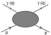
Figure 1: Forward Compton scattering of photons $\gamma(q)$ on protons $p$.

where $p\cdot q=M_{{\mbox{\scriptsize\rm p}}}\nu$, depends on two scalar invariant amplitudes of the squared energy $\nu^{2}$:

$$A(\nu)=f_{1}(\nu^{2})\vec{\epsilon^{\prime}}\cdot\vec{\epsilon}+\nu f_{2}(\nu^{2})i\vec{\sigma}\cdot\vec{\epsilon^{\prime}}\times\vec{\epsilon}.$$ (2)

The spin–flip amplitude obeys a dispersion relation which is expected to have no subtractions i.e.,

$$\mbox{\rm Re}f_{2}(\nu^{2})={\mbox{\rm PP}}\!\int_{0}^{\infty}\frac{d\tilde{\nu}^{2}}{\tilde{\nu}^{2}-\nu^{2}}\,\frac{1}{\pi}\mbox{\rm Im}f_{2}(\tilde{\nu}^{2}).$$ (3)

[Section 3 will be dedicated to the study of dispersion relations in general. They are the basics of sum rule derivations.] The optical theorem relates $\mbox{\rm Im}f_{2}(\nu^{2})$ to total cross–sections:

$$8\pi\,\mbox{\rm Im}f_{2}(\nu^{2})=\sigma_{\gamma{\mbox{\rm p}}}^{\uparrow\downarrow}(\nu)-\sigma_{\gamma{\mbox{\rm p}}}^{\uparrow\uparrow}(\nu),$$ (4)

and the low energy–theorem relates $\mbox{\rm Re}f_{2}(0)$ to the proton anomalous magnetic moment squared:

$$f_{2}(0)=-\frac{1}{2}\frac{\alpha}{M_{{\mbox{\scriptsize\rm p}}}^{2}}\left[F_{2}(0)\right]^{2}.$$ (5)

The optical theorem is a general property of unitarity in quantum field theory. The low–energy theorem follows from chiral symmetry properties of the underlying QCD Lagrangian [See the lectures of Pich [1] and Manohar [2] in this school.] The dispersion relation for forward scattering amplitudes is also a general property of quantum field theory [6]. What is still lacking to promote this sum rule to the status of a QCD theorem is the proof that $\mbox{\rm Im}f_{2}(\nu^{2})\rightarrow 0$ when $\nu\rightarrow\infty$. At present this accepted behaviour is only supported by theoretical strong interaction wisdom, like Regge phenomenology.

The Drell–Hearn sum rule has been checked in perturbation theory in QED–like theories to the first non–trivial order. One may ask if this sum rule could be used for practical calculations of the anomalous magnetic moment of the electron. The answer is that it is not a competitive method, simply because $F_{2}(0)$ in the l.h.s. appears squared which obliges one to calculate the integral in the r.h.s. to very high orders in powers of the fine structure constant.

The Drell–Hearn sum rule is also useful in the phenomenological study of deep inelastic scattering of polarized leptons on polarized protons [See Manohar’s lectures [2] in this school.], where it provides a constraint on the limit of real photoabsorption. It plays an important rôle as well in the calculation of the so called polarizability contribution to the hyperfine splitting in the hydrogen atom [See e.g. ref. [7] and references therein.]

2 The Adler–Weisberger Sum Rule

The sum rule in question [8, 9] relates the axial coupling constant $g_{\mbox{\scriptsize\rm A}}$ of $\beta$–decay to integrals of pion–nucleon total cross–sections:

$$1-g_{\mbox{\scriptsize\rm A}}^{2}=\frac{2f_{\pi}^{2}}{\pi}\int_{0}^{\infty}\frac{d\nu}{\nu}\left[\sigma_{\mbox{\scriptsize\rm tot}}^{\pi^{-}{\mbox{\scriptsize\rm p}}}(\nu)-\sigma_{\mbox{\scriptsize\rm tot}}^{\pi^{+}{\mbox{\scriptsize\rm p}}}(\nu)\right],$$ (6)

where $f_{\pi}\simeq 92\,\mbox{\rm MeV}$ denotes the pion decay coupling constant. The reference amplitude in this case is the forward pion–nucleon scattering amplitude illustrated in Fig. 2

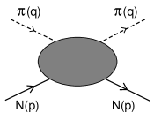
Figure 2: Forward pion–nucleon scattering amplitude.

which has two invariant amplitudes:

$$T_{ij}(\nu)=\delta_{ij}\,T^{(+)}(\nu)+\frac{1}{2}\left[\tau_{i},\tau_{j}\right]\,\frac{M_{\mbox{\scriptsize\rm p}}\nu}{f_{\pi}^{2}}T^{(-)}(\nu),$$ (7)

where $i,j$ are isospin indices. The basic dispersion relation is the one obeyed by the isospin–odd amplitude $T^{(-)}(\nu)$, and as in the case of the Compton scattering spin–flip amplitude, it is expected that $T^{(-)}(\nu)$ obeys an unsubtracted dispersion relation. The optical theorem relates $\mbox{\rm Im}T^{(-)}(\nu)$ to the difference of $\pi^{-}$–p and $\pi^{+}$–p total cross–sections. On the other hand, the calculation of the low–energy behaviour of the amplitude $\mbox{\rm Re}T^{(-)}(\nu)$ can be done using baryon chiral perturbation theory [2, 1]. The relevant Feynman diagrams are those of the Born approximation shown in Fig. 3

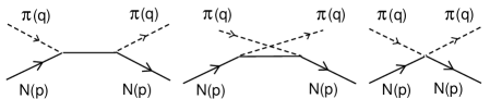
Figure 3: Forward pion–nucleon scattering at the Born approximation.

with the result

$$\lim_{\nu\rightarrow 0}\mbox{\rm Re}T^{(-)}(\nu)=1-g_{\mbox{\scriptsize\rm A}}^{2}.$$ (8)

The seagull graph contributes the factor 1, each one of the other graphs a factor $-\frac{1}{2}g_{\mbox{\scriptsize\rm A}}^{2}$.

Sometimes, the Adler–Weisberger sum rule is also written in the following way

$$1-\frac{1}{g_{\mbox{\scriptsize\rm A}}^{2}}=\frac{2M_{\mbox{\scriptsize\rm N}}^{2}}{\pi g_{\pi\mbox{\scriptsize\rm N}\mbox{\scriptsize\rm N}}^{2}}\,\int_{0}^{\infty}\frac{d\nu}{\nu}\left[\sigma_{\mbox{\scriptsize\rm tot}}^{\pi^{+}{\mbox{\scriptsize\rm p}}}(\nu)-\sigma_{\mbox{\scriptsize\rm tot}}^{\pi^{-}{\mbox{\scriptsize\rm p}}}(\nu)\right].$$ (9)

Both forms are equivalent, because of the Goldberger–Treiman relation [10]

$$g_{\mbox{\scriptsize\rm A}}M_{\mbox{\scriptsize\rm N}}=g_{\pi\mbox{\scriptsize\rm N}\mbox{\scriptsize\rm N}}f_{\pi}.$$ (10)

The Goldberger–Treiman relation is also a low–energy theorem of QCD.

I would like to come back to the question of an unsubtracted dispersion relation for the isospin–odd amplitude $T^{(-)}(\nu)$. This, of course depends on the high–energy behaviour of the underlying theory. One can consider as a toy model the linear sigma model [11] for constituent quarks. It has been shown [12, 13] that in perturbation theory, this model does not require subtractions in the corresponding Adler–Weisberger sum rule and yields, at the one–loop level, the result

$$g_{\mbox{\scriptsize\rm A}}^{2}=1-2\frac{M_{Q}^{2}}{16\pi^{2}f_{\pi}^{2}}\left(\log\frac{M_{\sigma}^{2}}{M_{Q}^{2}}+{\cal O}(1)\right),$$ (11)

where $M_{Q}$ denotes the mass of the constituent quark in this model. On the other hand, if one considers an effective constituent chiral quark model like the Georgi–Manohar model [14], then it can be shown [15] that the corresponding isospin–odd amplitude $T^{(-)}$ does not obey an unsubtracted dispersion relation. Beyond the tree level, $\mbox{\rm Re}T^{(-)}(\nu)$ cannot be obtained from a dispersive integral; and indeed, the calculation at the one–loop level reproduces the result in eq. (11) but with a cut–off replacing the sigma mass. It is simply that in this case the effective low–energy theory does not have the high–energy behaviour of the underlying theory.

3 The Weinberg Sum Rules

There is a correlation function which is particularly sensitive to properties of chiral symmetry breaking, namely the two–point function

$$\Pi_{LR}^{\mu\nu}(q)=2i\int d^{4}x\,e^{iq\cdot x}\langle 0|\mbox{\rm T}\left(L^{\mu}(x)R^{\nu}(0)^{\dagger}\right)|0\rangle,$$ (12)

with currents

$$L^{\mu}=\bar{d}(x)\gamma^{\mu}\frac{1}{2}(1-\gamma_{5})u(x)\quad\mbox{\rm and}\quad R^{\mu}=\bar{d}(x)\gamma^{\mu}\frac{1}{2}(1+\gamma_{5})u(x)\,.$$ (13)

In the chiral limit where the light quark masses are set to zero, this two–point function only depends on one invariant amplitude ($Q^{2}\equiv-q^{2}\geq 0$ for $q^{2}$ spacelike)

$$\Pi_{LR}^{\mu\nu}(Q^{2})=(q^{\mu}q^{\nu}-g^{\mu\nu}q^{2})\Pi_{LR}(Q^{2}).$$ (14)

The function $\Pi_{LR}(Q^{2})$ vanishes order by order in perturbation theory and is an order parameter of the spontaneous breakdown of chiral symmetry (S$\chi$SB) for all values of the momentum transfer. As illustrated in Fig. 4

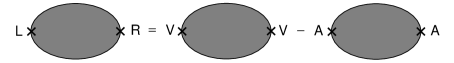
Figure 4: The $LR$ two–point function is the difference of $VV$ and $AA$ two–point functions.

the two–point function in eq. (12) is the difference of a vector current correlation function and an axial–vector current correlation function. Chiral symmetry identifies these two correlation functions.

Two–point functions in general obey dispersion relations. [See the discussion in section 3.] In 1967, and therefore prior to the development of QCD, Weinberg made an educated guess about the convergence properties of the LR two–point function, with the suggestion that the following two sum rules may hold in the underlying theory of the strong interactions [16]:

$$\int_{0}^{\infty}dt\mbox{\rm Im}\Pi_{LR}(t)\equiv\int_{0}^{\infty}dt\left[\mbox{\rm Im}\Pi_{V}(t)-\mbox{\rm Im}\Pi_{A}(t)\right]=0,$$ (15)

and

$$\int_{0}^{\infty}dt\,t\mbox{\rm Im}\Pi_{LR}(t)\equiv\int_{0}^{\infty}dt\,t\left[\mbox{\rm Im}\Pi_{V}(t)-\mbox{\rm Im}\Pi_{A}(t)\right]=0.$$ (16)

They are commonly referred to as the 1st Weinberg sum rule and the 2nd Weinberg sum rule, and they are examples of the so called superconvergent sum rules for the following reason. Let us assume that the function $\Pi_{LR}(Q^{2})$ obeys an unsubtracted dispersion relation:

$$\Pi_{LR}(Q^{2})=\int_{0}^{\infty}\frac{dt}{t+Q^{2}}\mbox{\rm Im}\Pi_{LR}(t).$$ (17)

The existence of the two sum rules above implies a stronger convergence behaviour for the function $\Pi_{LR}(Q^{2})$ in the deep euclidean region than the minimum required for the unsubtracted dispersion relation to hold. Expanding $\frac{1}{t+Q^{2}}=\frac{1}{Q^{2}}-\frac{1}{Q^{2}}t\frac{1}{Q^{2}}+\cdots$, we observe that the 1st Weinberg sum rule corresponds to the constraint

$$\lim_{Q^{2}\rightarrow\infty}Q^{2}\Pi_{LR}(Q^{2})\Rightarrow 0,$$ (18)

and the 2nd Weinberg sum rule to the further constraint

$$\lim_{Q^{2}\rightarrow\infty}Q^{4}\Pi_{LR}(Q^{2})\Rightarrow 0.$$ (19)

It is quite remarkable that, as we shall see in section 3, both constraints are now QCD properties; and in fact, the 1st Weinberg sum rule still holds in the presence of finite light quark masses [17].

I would like to make some comments on these sum rules.

i) Weinberg in his original paper [16] assumed that only the lowest narrow resonant state in the vector and axial–vector spectral functions:

$$\frac{1}{\pi}\mbox{\rm Im}\Pi_{V}(t)=f_{V}^{2}M_{V}^{2}\delta(t-M_{V}^{2})+\cdots$$ (20)

and

$$\frac{1}{\pi}\mbox{\rm Im}\Pi_{A}(t)=f_{\pi}^{2}\delta(t)+f_{A}^{2}M_{A}^{2}\delta(t-M_{A}^{2})+\cdots,$$ (21)

contribute significantly to the sum rules. The first term in the axial–vector spectral function in eq. (21) is the contribution from the massless pion. Thus the 1st and 2nd Weinberg sum rules in eqs.(15) and (16) constrain the couplings and masses of the narrow resonances as follows

$$\begin{split}f_{V}^{2}M_{V}^{2}-f_{A}^{2}M_{A}^{2}&=f_{\pi}^{2}\\ f_{V}^{2}M_{V}^{4}-f_{A}^{2}M_{A}^{4}&=0.\end{split}$$ (22)

It is interesting that the original Weinberg’s ansatz in eqs. (20) and (21) can now be justified within the framework of the large–$N_{c}$ limit of QCD. Indeed, in this limit, the vector and axial–vector spectral functions are each a sum of an infinite number of narrow sates. The dots in the spectral functions in eqs. (20) and (21) implicitly assume that the sum of the rest of the narrow states is already globally dual to the onset of the perturbative continuum,

$$\frac{1}{\pi}\mbox{\rm Im}\Pi_{V}(t)=f_{V}^{2}M_{V}^{2}\delta(t-M_{V}^{2})+\frac{N_{c}}{16\pi^{2}}\frac{2}{3}\theta(t-s_{0})[1+\cdots],$$ (23)

and

$$\frac{1}{\pi}\mbox{\rm Im}\Pi_{A}(t)=f_{\pi}^{2}\delta(t)+f_{A}^{2}M_{A}^{2}\delta(t-M_{A}^{2})+\frac{N_{c}}{16\pi^{2}}\frac{2}{3}\theta(t-s_{0})[1+\cdots],$$ (24)

where the dots indicate now gluonic corrections. The vector and axial–vector spectral functions of the pQCD continuum are the same in the chiral limit.

ii) In order to make a “prediction” for the axial mass $M_{A}$, Weinberg in his original paper also makes the assumption that

$$f_{V}^{2}=2\frac{f_{\pi}^{2}}{M_{V}^{2}},$$ (25)

which was called at the time the KSFR relation [18, 19]. This, together with eqs. (22) leads to the prediction $M_{A}=\sqrt{2}M_{V}$ which is satisfied by the central values of the presently known masses within an accuracy of less than $\sim 12\%$. It can be shown [20] that the KSFR–relation follows from the assumption that both the electromagnetic pion form factor and the axial form factor in $\pi\rightarrow e\nu_{e}\gamma$ obey unsubtracted dispersion relations, plus the dynamical input of resonance dominance.

iii) Inverse moments of the difference of vector and axial–vector spectral functions with the pion pole removed, i.e. integrals like

$$\int_{0}^{\infty}dt\frac{1}{t^{p}}\left(\frac{1}{\pi}\mbox{\rm Im}\Pi_{LR}(t)+f_{\pi}^{2}\delta(t)\right),$$ (26)

with $p=1,2,3,\cdots$, correspond to non–local order parameters which govern the couplings of local operators of higher and higher dimensions in the low energy effective chiral Lagrangian [See Pich’s lectures [1] in this school.]. For example, the first inverse moment is related to the ${\cal O}(p^{4})$ coupling constant $L_{10}$ as follows [21]

$$-4L_{10}=\int_{0}^{\infty}\frac{dt}{t}\,\left(\frac{1}{\pi}\mbox{\rm Im}\Pi_{V}(t)-\frac{1}{\pi}\mbox{\rm Im}\tilde{\Pi}_{A}(t)\right),$$ (27)

where the tilde in $\mbox{\rm Im}\tilde{\Pi}$ indicates that the pion pole has been removed. Using the ansatz in eqs. (23) and (24) and the two Weinberg sum rules in eq. (22) one finds

$$-4L_{10}=f_{V}^{2}-f_{A}^{2}=f_{\pi}^{2}\left(\frac{1}{M_{V}^{2}}+\frac{1}{M_{A}^{2}}\right),$$ (28)

which provides a good estimate [20] of the $L_{10}$ coupling constant.

iv) One of the parameters which characterize possible deviations from the Standard Model predictions in the electroweak sector is the so called $S$–parameter [See the lectures of Treille [22] and Chivukula [23] in this school.]. In the unitary gauge, $S$ measures the strength of an anomalous $W^{(3)}_{\mu\nu}B^{\mu\nu}$ coupling. This is the $SU(2)_{L}\times SU(2)_{R}$ coupling analogous to the term proportional to $L_{10}$ in QCD. It has been argued that if the underlying theory of electroweak breaking is a vector–like gauge theory of the QCD–type, the sign of the $L_{10}$–like coupling must be negative, precisely as observed in QCD. In the electroweak sector, this fact is infirmed by experimental observation and constitutes at present a serious phenomenological obstacle to technicolour–like formulations of electroweak symmetry breaking. The relation of the $L_{10}$ coupling to the relative size of local order parameters versus $f_{\pi}^{2}$ in the large–$N_{c}$ limit of QCD–like theories has been recently discussed in ref. [24].

4 The Electromagnetic Pion Mass Difference

The most remarkable application of the Weinberg sum rules is the calculation of the $\pi^{+}-\pi^{0}$ electromagnetic mass difference [25]. In the chiral limit and to lowest order in the electromagnetic interactions, there appears a new term with no derivatives in the low–energy effective chiral Lagrangian [26]

$${\cal L}_{\mbox{\scriptsize\rm eff}}=\cdots+e^{2}C\,\mbox{\rm tr}\left(Q_{R}UQ_{L}U^{\dagger}\right),$$ (29)

where $U$ is the matrix field which collects the octet of pseudoscalar Goldstone fields [See Pich’s lectures [1] in this school.] and $Q_{R}=Q_{L}=\mbox{\rm diag}[2/3,-1/3,-1/3]$ the right– and left–charges associated with the electromagnetic couplings of the light quarks. Expanding $U$ in powers of the pseudoscalar fields there appear quadratic terms like

$${\cal L}_{\mbox{\scriptsize\rm eff}}=\cdots-2e^{2}C\frac{1}{f_{\pi}^{2}}(\pi^{+}\pi^{-}+K^{+}K^{-})+\cdots,$$ (30)

showing that, in the presence of electromagnetic interactions, the charged pion and kaon fields become massive:

$$(m_{K^{+}}^{2}-m_{K^{0}}^{2})|_{\mbox{\scriptsize\rm EM}}=(m_{\pi^{+}}^{2}-m_{\pi^{0}}^{2})|_{\mbox{\scriptsize\rm EM}}=\frac{2e^{2}C}{f_{\pi}^{2}}.$$ (31)

In fact, the main contribution to the physical $\pi^{+}$–$\pi^{0}$ mass difference is of electromagnetic origin because quark masses do not contribute significantly to the $\pi^{+}$–$\pi^{0}$ mass splitting.

It can be formally shown [See e.g. refs. [27, 28] and references therein.] that the coupling constant $C$ of the effective term in eq. (29) which results from the integration of a virtual photon of euclidean momentum squared $Q^{2}$ in the presence of the strong interactions in the chiral limit, is given by an integral of the correlation function $\Pi_{LR}(Q^{2})$ defined in eqs. (12) and (14):

$$C=\frac{-1}{8\pi^{2}}\,\frac{3}{4}\,\int_{0}^{\infty}dQ^{2}\,Q^{2}\Pi_{LR}(Q^{2}).$$ (32)

The constraints in eqs. (18) and (19) guarantee the convergence of the integral in the ultraviolet. Inserting the resonance dominance ansatz in eqs. (23) and (24) for the vector and axial–vector spectral functions in the dispersion integral representation in eq. (17) results in

$$\Pi_{LR}(Q^{2})=-\frac{f_{\pi}^{2}}{Q^{2}}-\frac{f_{A}^{2}M_{A}^{2}}{M_{A}^{2}+Q^{2}}+\frac{f_{V}^{2}M_{V}^{2}}{M_{V}^{2}+Q^{2}}.$$ (33)

With this expression inserted in the integrand of the r.h.s. in eq. (32) and using the 1st and 2nd Weinberg sum rules in eqs. (22) one easily obtains

$$(m_{\pi^{+}}^{2}-m_{\pi^{0}}^{2})|_{\mbox{\scriptsize\rm EM}}=\frac{\alpha}{\pi}\frac{3}{4}\frac{M_{A}^{2}M_{V}^{2}}{M_{A}^{2}-M_{V}^{2}}\log\frac{M_{A}^{2}}{M_{V}^{2}}.$$ (34)

The authors of ref. [25] also use $M_{A}=\sqrt{2}M_{V}$ which results in

$$(m_{\pi^{+}}^{2}-m_{\pi^{0}}^{2})|_{\mbox{\scriptsize\rm EM}}=\frac{\alpha}{\pi}\frac{3}{2}\,M_{\rho}^{2}\,\log 2.$$ (35)

Numerically, this corresponds to a mass difference $\Delta m_{\pi}|_{\mbox{\scriptsize\rm EM}}\simeq 5.2\,\mbox{\rm MeV}$ to be compared with the experimental mass difference $m_{\pi^{+}}-m_{\pi^{0}}=4.6\,\mbox{\rm MeV}$.

Equation (32) can nowadays be viewed as a rigorous QCD sum rule in the chiral limit. The sum rule relates the low–energy constant $(m_{\pi^{+}}^{2}-m_{\pi^{0}}^{2})|_{\mbox{\scriptsize\rm EM}}$ to an integral of the real part of a two–point function. The integral runs over all possible values of the euclidean momenta and therefore it requires, a priori, the knowledge of the two–point function at all distances. I want to stress the fact that it is not enough to know the very low $Q^{2}$ behaviour of the $\Pi_{LR}(Q^{2})$ correlation function to obtain an approximation to the r.h.s. integral in eq (32). The low $Q^{2}$ behaviour of this function is governed by chiral perturbation theory and the first two terms are known

$$\Pi_{LR}(Q^{2})=-\frac{f_{\pi}^{2}}{Q^{2}}-4L_{10}+{\cal O}(Q^{2});$$ (36)

but this behaviour cannot be extrapolated to the ultraviolet region of the integral since it would lead to a divergent result. By contrast, as we shall further discuss in section 3, the full $Q^{2}$ resonance dominance ansatz in eq. (33) with the Weinberg sum rule constraints in eqs. (22) has both the long–distance behaviour and the short–distance behaviour of QCD.

3 Dispersion Relations

In these lectures we shall be all the time considering two–point functions of local operators i.e., Fourier transforms of the vacuum expectation value of the time ordered product of a local current $J(x)$ times its hermitian conjugate

$$\Pi(q^{2})=i\int d^{4}xe^{iq\cdot x}\langle 0|\mbox{\rm T}\left\{J(x)J(0)^{\dagger}\right\}|0\rangle.$$ (37)

In most applications the current $J(x)$ is one of the Noether currents associated with global gauge transformations of flavour degrees of freedom, like a vector current $\bar{q}(x)\gamma^{\mu}q(x)$, or an axial–vector current $\bar{q}(x)\gamma^{\mu}\gamma_{5}q(x)$; but one could also consider gauge invariant local operators of gluon fields like $\mbox{\rm tr}G^{\mu\nu}(x)G_{\mu\nu}(x)$, or composite operators like $\bar{q}(x)\Gamma q(x)\bar{q}(x)\Gamma q(x)$. It has been shown by Källén and Lehmann [29, 30] quite a long time ago that two–point functions obey dispersion relations. The dispersion relation follows from the analyticity properties of $\Pi(q^{2})$ as a complex function of $q^{2}$, the only energy–momentum invariant which appears in a two–point function. In full generality $\Pi(q^{2})$ is an analytic function in the complex $q^{2}$–plane but for a cut in the real axis $0\leq q^{2}\leq\infty$. It then follows that

$$\Pi(q^{2})=\int_{0}^{\infty}dt\frac{1}{t-q^{2}-i\epsilon}\frac{1}{\pi}\mbox{\rm Im}\Pi(t)+\mbox{\rm a}+\mbox{\rm b}q^{2}+\cdots,$$ (38)

where the degree of the arbitrary polynomial in the r.h.s. depends on the convergence properties of $\mbox{\rm Im}\Pi(t)$ when $t\rightarrow\infty$. The interest of this representation is that $\frac{1}{\pi}\mbox{\rm Im}\Pi(t)$ in the integrand, which is usually called the spectral function, is a physical cross–section. With $J(x)$ a current with specific quantum numbers, the spectral function is then directly related to the total cross section for the production from the vacuum of hadronic states with those quantum numbers.

For example, with $J$ the electromagnetic hadronic current of light quarks,

$$J^{\mu}(x)=\frac{2}{3}\bar{u}(x)\gamma^{\mu}u(x)-\frac{1}{3}\bar{d}(x)\gamma^{\mu}d(x)-\frac{1}{3}\bar{s}(x)\gamma^{\mu}s(x)$$ (39)

the relation to the total $e^{+}e^{-}$ annihilation cross–section into hadrons is

$$\sigma(q^{2})_{e^{+}e^{-}\rightarrow\mbox{\rm hadrons}}=\frac{4\pi^{2}\alpha}{q^{2}}\,e^{2}\frac{1}{\pi}\mbox{\rm Im}\Pi_{\mbox{\tiny\rm EM}}(q^{2}),$$ (40)

and

$$\begin{split}-3\theta(q)q^{2}&\,\frac{1}{\pi}\mbox{\rm Im}\Pi_{\mbox{\tiny\rm EM}}(q^{2})=\\ &\sum_{\Gamma}\langle 0|J^{\mu}_{\mbox{\tiny\rm EM}}(0)|\Gamma\rangle\langle\Gamma|J_{\mu,\mbox{\tiny\rm EM}}(0)^{\dagger}|0\rangle(2\pi)^{3}\delta^{(4)}(q-p_{\Gamma}),\end{split}$$ (41)

where the sum is extended to all possible physical states, on–shell states, with an integration over their corresponding phase space understood. A pictorial representation of these equations is shown in Fig. 5 below.

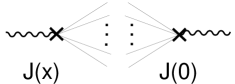
Figure 5: Representation of the hadronic spectral function in eq. (41).

The lowest possible state in this case is a two–pion state. The function $\Pi_{\mbox{\tiny\rm EM}}(q^{2})$ is analytic in the complex $q^{2}$–plane but for a cut in the real axis: $4m_{\pi}^{2}\leq q^{2}\leq\infty$, as illustrated in Fig. 6.

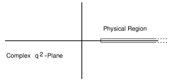
Figure 6: Representation of the complex $q^{2}$–plane.

I want to show first how these properties appear explicitly in a simple case which you should be familiar with, and then we shall discuss a general proof.

1 Vacuum Polarization due to Massive Fermions

Let us consider QED with a massive fermion. We want to calculate the lowest order vacuum polarization contribution from this fermion, i.e. the one–loop Feynman diagram in Fig. 7.

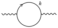
Figure 7: One fermion loop contribution to vacuum polarization.

Combining the two fermion propagators with a Feynman parameter $x$,

$$\frac{1}{AB}=\int_{0}^{1}\frac{1}{[Ax+B(1-x)]^{2}},$$ (42)

and after integration over the four–momenta $k$ in the loop [I am assuming that a gauge invariant regularization of this integral, like e.g. dimensional regularization, has been made.], the one–particle irreducible part of this diagram, when subtracted at $q^{2}=0$ if we choose on–shell renormalization, leads to the renormalized self–energy function:

$$\Pi_{\mbox{\tiny\rm R}}(q^{2})=-\frac{\alpha}{\pi}\int_{0}^{1}dx\,2x(1-x)\log\left(1-\frac{q^{2}}{m^{2}-i\epsilon}x(1-x)\right),$$ (43)

With the change of variables $y=1-2x$, and using the fact that the resulting integral is symmetric when $y\rightarrow-y$, we get

$$\Pi_{\mbox{\tiny\rm R}}(q^{2})=\frac{\alpha}{\pi}\int_{0}^{1}dy(1-y^{2})\log\left[1-\frac{q^{2}}{4m^{2}-i\epsilon}(1-y^{2})\right].$$ (44)

Integrating by parts this equation using the identity: $1-y^{2}=\frac{\partial}{\partial y}(y-\frac{1}{3}y^{3})$ results in a rational integral:

$$\Pi_{\mbox{\tiny\rm R}}(q^{2})=\frac{\alpha}{\pi}\int_{0}^{1}dy\,2y(y-\frac{1}{3}y^{3})\frac{q^{2}}{4m^{2}-q^{2}(1-y^{2})-i\epsilon},$$ (45)

and with a new change of variables: $t=\frac{4m^{2}}{1-y^{2}}$ we finally get a rather interesting representation of the renormalized self–energy

$$\frac{\Pi_{\mbox{\tiny\rm R}}(q^{2})}{q^{2}}=\frac{\alpha}{\pi}\int_{4m^{2}}^{\infty}\frac{dt}{t}\,\frac{1}{t-q^{2}-i\epsilon}\,\frac{1}{3}\left(1+\frac{2m^{2}}{t}\right)\sqrt{1-\frac{4m^{2}}{t}}.$$ (46)

The reason why this representation is interesting is that it is in fact a dispersion relation! We have succeeded in rewriting the initial Feynman parametric representation in eq. (43) as a dispersion relation by simple changes of variables. Using the identity

$$\frac{1}{t-q^{2}-i\epsilon}=\mbox{\rm PP}\frac{1}{t-q^{2}}+i\pi\delta(t-q^{2}),$$ (47)

we immediately see that

$$\frac{1}{\pi}\mbox{\rm Im}\Pi(t)=\frac{\alpha}{\pi}\frac{1}{3}\left(1+\frac{2m^{2}}{t}\right)\sqrt{1-\frac{4m^{2}}{t}}\theta(t-4m^{2}).$$ (48)

Equation (46) is a particular case of the general dispersion relation written in eq. (38), when the arbitrary polynomial is just a constant, and we have got rid of the constant because the on–shell renormalized $\Pi_{\mbox{\tiny\rm R}}$ is defined as

$$\Pi_{\mbox{\tiny\rm R}}(q^{2})=\Pi(q^{2})-\Pi(0)=\int_{0}^{\infty}\frac{dt}{t}\,\frac{q^{2}}{t-q^{2}-i\epsilon}\,\frac{1}{\pi}\mbox{\rm Im}\Pi(t).$$ (49)

It is perhaps worth insisting on the fact that asymptotically

$$\lim_{t\rightarrow\infty}\frac{1}{\pi}\mbox{\rm Im}\Pi(t)\Rightarrow\frac{\alpha}{\pi}\frac{1}{3};$$ (50)

i.e. the electromagnetic spectral function goes to a constant. In fact, it is this constant which fixes the value of the lowest order contribution to the $\beta$–function associated with charge renormalization in QED.

2 General Proof of Dispersion Relations

We shall now sketch a proof of the dispersion relation property for two–point functions in full generality. The key of the proof lies in the definition of the time ordered product implicit in eq. (37):

$$\mbox{\rm T}(J(x)J(0)^{\dagger}=\theta(x)J(x)J(0)^{\dagger}+\theta(-x)J(0)^{\dagger}J(x),$$ (51)

and the use of translation invariance. The function $\theta(x)$ is the Heaviside function: $\theta(x)=1$ if $x_{0}>0$ and $\theta(x)=0$ if $x_{0}<0$, which has the integral representation

$$\theta(x)=\frac{1}{2\pi i}\int_{-\infty}^{+\infty}dw\,\frac{e^{iwx}}{w-i\epsilon}.$$ (52)

First we insert a complete set of states $\sum_{\Gamma}|\Gamma\rangle\langle\Gamma|$ between the two currents in the T–product definition. This leads to matrix elements of the type $\langle 0|J(x)|\Gamma\rangle$ to which we apply translation invariance:

$$\langle 0|J(x)|\Gamma\rangle=\langle 0|{\cal U}^{-1}{\cal U}J(x){\cal U}^{-1}{\cal U}|\Gamma\rangle,$$ (53)

where ${\cal U}$ is the unitary operator induced by translations in space–time:

$${\cal U}(a)J(x){\cal U}^{-1}(a)=J(x+a)\quad\mbox{\rm and}\quad{\cal U}(a)|\Gamma\rangle=e^{ip_{\Gamma}\cdot a}|\Gamma\rangle,$$ (54)

and $p_{\Gamma}$ denotes the sum of the energy–momenta of all the particles which define the state $|\Gamma\rangle$. The choice $a\equiv-x$ factors out the $x$–dependence of the matrix element into an exponential:

$$\langle 0|J(x)|\Gamma\rangle=e^{-ip_{\Gamma}\cdot x}\,\langle 0|J(0)|\Gamma\rangle.$$ (55)

All the particles in the state $|\Gamma\rangle$ are on–shell. This constrains the total energy–momentum $p_{\Gamma}$ to be a time–like vector: $p_{\Gamma}^{2}=t$ with $t\geq 0$. With these constrains on $p_{\Gamma}$ we can insert the identity

$$\int_{0}^{\infty}dt\int d^{4}p\,\theta(p)\,\delta(p^{2}-t)\,\delta^{(4)}(p-p_{\Gamma})=1$$ (56)

inside the sum $\sum_{\Gamma}$ over the complete set of states. Interchanging the order of sum over $\Gamma$ and integration over $t$ and $p$, there appears naturally the definition of the spectral function associated with the $J$–operator

$$\sum_{\Gamma}\langle 0|J(0)|\Gamma\rangle\langle\Gamma|J(0)^{\dagger}|0\rangle\,(2\pi)^{4}\delta^{(4)}(p-p_{\Gamma})\equiv 2\pi\rho(p^{2}).$$ (57)

The spectral function $\rho(p^{2})$ is a scalar function of the Lorentz invariant $p^{2}$ and the masses of the particles in the states $|\Gamma\rangle$ only. By construction it is a real function and non–negative

$$\rho(p^{2})^{*}=\rho(p^{2})\geq 0.$$ (58)

We can now rewrite the two–point function in eq. (37) as follows

$$\begin{split}\Pi&(q^{2})=\int d^{4}x\,e^{iq\cdot x}\int_{0}^{\infty}dt\,\rho(t)\times\\ &\int\frac{d^{4}p}{(2\pi)^{3}}\left[i\theta(x)\,e^{-ip\cdot x}\theta(p)\delta(p^{2}-t)+i\theta(-x)\,e^{ip\cdot x}\theta(p)\delta(p^{2}-t)\right].\end{split}$$ (59)

Here, you may recognize the familiar functions of free field theory

$$\Delta^{+}(x)=\int\frac{d^{4}p}{(2\pi)^{3}}\,e^{-ip\cdot x}\theta(p)\delta(p^{2}-t)$$ (60)

and

$$\begin{split}\Delta^{-}(x)&=\int\frac{d^{4}p}{(2\pi)^{3}}\,e^{ip\cdot x}\theta(p)\delta(p^{2}-t)\\ &=\int\frac{d^{4}p}{(2\pi)^{3}}\,e^{-ip\cdot x}\theta(-p)\delta(p^{2}-t);\end{split}$$ (61)

and therefore the Feynman propagator function

$$\begin{split}\Delta_{\mbox{\small\rm F}}(x;t)&=i\theta(x)\Delta^{+}(x;t)+i\theta(-x)\Delta^{-}(x;t)\\ &=\int\frac{d^{4}p}{(2\pi)^{4}}\frac{e^{-ip\cdot x}}{t-p^{2}-i\epsilon},\end{split}$$ (62)

where the last expression can be obtained using the representation in eq. (52) of the $\theta$–function [See e.g. ref. [31] pp. 50-51.]. The two–point function $\Pi(q^{2})$ appears then to be the Fourier transform of a scalar free field propagating with an arbitrary mass squared $t$ weighted by the spectral function density $\rho(t)$ and integrated over all possible values of $t$,

$$\Pi(q^{2})=\int d^{4}x\,e^{iq\cdot x}\int_{0}^{\infty}dt\,\rho(t)\,\Delta_{\mbox{\small\rm F}}(x;t).$$ (63)

Integrating over $x$ and $p$ results finally in the wanted representation

$$\Pi(q^{2})=\int_{0}^{\infty}dt\,\rho(t)\frac{1}{t-q^{2}-i\epsilon}.$$ (64)

With

$$\Pi(q^{2})=\mbox{\rm Re}\Pi(q^{2})+i\mbox{\rm Im}\Pi(q^{2}),$$ (65)

and the use of the identity in eq. (47), it follows that

$$\rho(t)\equiv\frac{1}{\pi}\mbox{\rm Im}\Pi(t),$$ (66)

which identifies the spectral function with the imaginary part of the two–point function.

Notice that the formal manipulations above avoid the question of convergence of the principal value integral

$$\mbox{\rm Re}\Pi(q^{2})=\mbox{\rm PP}\!\int_{0}^{\infty}dt\,\frac{1}{t-q^{2}}\,\frac{1}{\pi}\mbox{\rm Im}\Pi(t).$$ (67)

The convergence of the integral in the ultraviolet limit ($t\rightarrow\infty$) depends on the behaviour of the spectral function at large $t$–values. When doing above the exchange of sum over $\Gamma$ and integrations we have implicitly assumed good convergence properties; but in general the product of the distributions $\theta(x)$ and $\int_{0}^{\infty}dt\,\rho(t)\,\Delta^{+}(x;t)$ may not be a well–defined distribution. The ambiguity manifests by the presence of an arbitrary polynomial in $q^{2}$ in the r.h.s. of the PP–integral

$$\mbox{\rm Re}\Pi(q^{2})=\mbox{\rm PP}\!\int_{0}^{\infty}dt\,\frac{1}{t-q^{2}}\,\frac{1}{\pi}\mbox{\rm Im}\Pi(t)+\mbox{\rm a}+\mbox{\rm b}q^{2}+\dots\,.$$ (68)

Notice that the coefficients of the arbitrary polynomial have no discontinuities; in other words, the ambiguity of short–distance behaviour reflects only in the evaluation of the real part of the two–point function, not in the imaginary part. The physical meaning of these coefficients depends of course on the choice of the local operator $J(x)$ in the two–point function. In some cases the coefficients in question are fixed by low–energy theorems; e.g. if $\Pi(0)$ is known, we can trade the constant a in eq. (68) for $\Pi(0)$:

$$\mbox{\rm Re}\Pi(q^{2})=\mbox{\rm Re}\Pi(0)+\mbox{\rm PP}\!\int_{0}^{\infty}\frac{dt}{t}\frac{q^{2}}{t-q^{2}}\,\frac{1}{\pi}\mbox{\rm Im}\Pi(t)+\mbox{\rm b}q^{2}+\dots\,.$$ (69)

In other cases the constants are absorbed by renormalization constants. In general, it is always possible to get rid of the polynomial terms by taking an appropriate number of derivatives with respect to $q^{2}$. Various examples will be discussed later.

3 QCD Moment Sum Rules

In QCD the number of derivatives which is required to obtain a well defined two–point function is fixed by the asymptotic freedom property of the theory. For a gauge invariant local operator $J(x)$, the asymptotic behaviour of the associated two–point function is of the type

$$\lim_{t\rightarrow\infty}\frac{1}{\pi}\mbox{\rm Im}\Pi(t)\Rightarrow{\mbox{\rm A}}t^{d}\left\{1+a_{1}\frac{\alpha_{\mbox{\rm{\scriptsize s}}}(t)}{\pi}+\dots\,\right\},$$ (70)

with A and $a_{1}$ calculable coefficients, and $d$ a known integer $d=0,1,2,\dots\,$, depending on the dimensions of the operator $J(x)$. It is then sufficient to take $d+1$ derivatives with respect to $q^{2}$ to get rid of the arbitrary polynomial and obtain a convergent integral. The functions defined by the moment integrals ($Q^{2}\equiv-q^{2}$):

$$\begin{split}\Pi^{(m)}(Q^{2})&=\frac{(-1)^{m}}{(m-d-1)!}\,(Q^{2})^{m-d}\,\frac{\partial^{m}}{(\partial Q^{2})^{m}}\,\Pi(q^{2})\\ &=\int_{0}^{\infty}dt\,\frac{m(m-1)\cdots(m-d)}{(t+Q^{2})^{d+1}}\,\left(\frac{Q^{2}}{t+Q^{2}}\right)^{m-d}\frac{1}{\pi}\mbox{\rm Im}\Pi(t),\end{split}$$ (71)

for $m\geq d+1$ are then well defined functions calculable in pQCD at sufficiently large $Q^{2}$–values.

4 The Adler Function

An example of a QCD moment sum rule is the Adler function corresponding to the two–point function associated with the vector–isovector quark current

$$V^{\mu}_{\mbox{\scriptsize\rm I}=1}(x)=\frac{1}{2}\left[:\!{\bar{u}}(x)\gamma^{\mu}u(x)\!:-:\!{\bar{d}}(x)\gamma^{\mu}d(x)\!:\right].$$ (72)

Since the current is conserved, the two–point function

$$\begin{split}\Pi_{\mbox{\scriptsize\rm I}=1}^{\mu\nu}(q)&=i\int d^{4}xe^{iq\cdot x}\langle 0|\mbox{\rm T}\left\{V_{\mbox{\scriptsize\rm I}=1}^{\mu}(x)V_{\mbox{\scriptsize\rm I}=1}^{\nu}(0)\right\}|0\rangle\\ &=-(g^{\mu\nu}q^{2}-q^{\mu}q^{\nu})\Pi_{\mbox{\scriptsize\rm I}=1}(q^{2}),\end{split}$$ (73)

has one invariant function $\Pi_{\mbox{\scriptsize\rm I}=1}(q^{2})$ only. Power counting tells us that in this case the asymptotic behaviour of the corresponding spectral function goes as a constant i.e. the power $d$ in the r.h.s. of eq. (70) is $d=0$. Only one derivative is required to have a well defined correlation function. The Adler function is defined as the logarithmic derivative of $\Pi(q^{2})_{\mbox{\scriptsize\rm I}=1}$ ($Q^{2}\equiv-q^{2}$, with $Q^{2}\geq 0$ for $q^{2}$–spacelike),

$${\cal A}(Q^{2})\equiv-Q^{2}\frac{\partial\Pi_{\mbox{\scriptsize\rm I}=1}(q^{2})}{\partial Q^{2}}.$$ (74)

This function, for sufficiently large values of $Q^{2}$ is calculable in pQCD as a power series in the running coupling constant. On the other hand the vector–isovector spectral function $\frac{1}{\pi}\mbox{\rm Im}\Pi_{\mbox{\scriptsize\rm I}=1}(t)$ is accessible to experimental determination from $e^{+}e^{-}$ annihilation into hadrons and from the $\tau$ hadronic decays. We then have the sum rule

$${\cal A}(Q^{2})=\int_{0}^{\infty}dt\,\frac{Q^{2}}{(t+Q^{2})^{2}}\,\frac{1}{\pi}\mbox{\rm Im}\Pi_{\mbox{\scriptsize\rm I}=1}(t).$$ (75)

When trying to confront this sum rule with experiment, there appears the problem that the integrand in the r.h.s. is only known experimentally from threshold up to finite values of $t$. This brings in a question of matching whatever is known about the low energy hadronic spectral function with its asymptotic behaviour as predicted by pQCD. We shall later on come back to this important question, after the discussion of non–perturbative power corrections.

The Adler function has been calculated in perturbation theory to the four-loop level [32, 33, 34, 35, 36]. In the $\overline{MS}$–scheme and with $\alpha_{\mbox{\rm{\scriptsize s}}}\equiv\alpha_{\overline{MS}}({Q^{2}})$, the numerical evaluation of the exact perturbative calculations for $N_{c}=3$ and for three light flavours $n_{f}=3$ gives the result

$${\cal A}(Q^{2})|_{\mbox{\scriptsize pert.}}=\frac{N_{c}}{16\pi^{2}}\frac{2}{3}\left\{1+\frac{\alpha_{s}}{\pi}+1.64\left(\frac{\alpha_{s}}{\pi}\right)^{2}+6.37\left(\frac{\alpha_{s}}{\pi}\right)^{3}\right\}.$$ (76)

4 Types of Two–Point Function Sum Rules

There are several types of sum rules which have been discussed in the literature. They differ on the way that the analyticity properties of two–point functions are exploited and/or on various limits that one can define on moment sum rules. We explain the most common types of sum rules below.

1 Laplace Transform Sum Rules

The Laplace transform of a spectral function:

$${\cal M}(\sigma)=\int_{0}^{\infty}dt\,e^{-t\sigma}\,\frac{1}{\pi}\mbox{\rm Im}\Pi(t),$$ (77)

is a calculable function in pQCD provided that the variable $\sigma$, which has the dimensions of an inverse mass squared, is sufficiently small. The interesting point about this type of sum rules is the presence of the exponential factor in the integrand which gives a predominant weight to the low–energy component of the hadronic spectral function compared to the power weight of a moment sum rule. Sum rules of this type were first proposed by the ITEP group [37] who called them Borel sum rules. The Laplace transform in (77) results from a precise limit of the moment sum rules discussed in section 3; it is the limit where the number of derivatives $N$ of the invariant two–point function $\Pi(q^{2})$ with respect to $Q^{2}$ and $Q^{2}\equiv-q^{2}$ both go to infinity with their ratio $\frac{Q^{2}}{N}\equiv M^{2}\equiv\frac{1}{\sigma}$ fixed. More precisely, the limit is obtained by applying the operator

$${\mbox{\bf L}}\equiv\lim_{N\rightarrow\infty}\lim_{Q^{2}\rightarrow\infty}|_{\frac{N}{Q^{2}}=\sigma}\,\frac{(-1)^{N}}{(N-1)!}\left(Q^{2}\right)^{N}\frac{\partial^{N}}{\left(\partial Q^{2}\right)^{N}}$$ (78)

to the first well–defined moment of $\Pi(q^{2})$, [ $d$ is the asymptotic power behaviour defined in eq. (70)]:

$$\begin{split}\frac{1}{\sigma}&{\mbox{\bf L}}\left[(-1)^{d+1}\frac{\partial^{d+1}}{\left(\partial Q^{2}\right)^{d+1}}\Pi(q^{2})\right]=\\ &\int_{0}^{\infty}dt\,\frac{N(N+1)\cdots(N+d+1)}{(t+Q^{2})^{d+1}}\,\frac{1}{\left(1+\frac{1}{N}t\frac{N}{Q^{2}}\right)^{N}}\,\frac{1}{\pi}\mbox{\rm Im}\Pi(t).\end{split}$$ (79)

In the limit which we are considering, the first fraction in the integrand goes to $\sigma^{d+1}$ and the second fraction to $e^{-t\sigma}$, with the result that

$$\frac{1}{\sigma}{\mbox{\bf L}}\left[(-1)^{d+1}\frac{\partial^{d+1}}{\left(\partial Q^{2}\right)^{d+1}}\Pi(q^{2})\right]\Rightarrow\sigma^{d+1}\int_{0}^{\infty}dt\,e^{-t\sigma}\,\frac{1}{\pi}\mbox{\rm Im}\Pi(t).$$ (80)

In practice, the question which then appears is how to calculate the function ${\cal M}(\sigma)$ without having to take the complicated limits which define the operator L in eq. (78). This is possible because L is nothing but an algebraic form of the Laplace inversion operator. Once this is recognized [38], it is easy to go directly from the moment sum rule

$$(-1)^{d+1}\frac{\partial^{d+1}}{\left(\partial Q^{2}\right)^{d+1}}\Pi(q^{2})=\int_{0}^{\infty}dt\,\frac{(d+1)!}{(t+Q^{2})^{d+2}}\,\frac{1}{\pi}\mbox{\rm Im}\Pi(t)$$ (81)

to the Laplace transform in (77). Indeed, the power weight in the integrand of eq. (81) can be written as a Laplace transform with respect to the variable $Q^{2}$

$$\frac{(d+1)!}{(t+Q^{2})^{d+2}}=\int_{0}^{\infty}dx\,e^{-xQ^{2}}\,x^{d+1}\,e^{-xt},$$ (82)

and the action of L brings back the inverse Laplace transform i.e.,

$${\mbox{\bf L}}\left[\frac{((d+1)!}{(t+Q^{2})^{d+2}}\right]=\sigma^{d+1}\,e^{-t\sigma}.$$ (83)

This provides the key to calculate the Laplace transform ${\cal M}(\sigma)$ once we know $\Pi(q^{2})$. The results of analytic pQCD calculations of self–energy functions like $\Pi(q^{2})$ are combinations of terms which are typically of the form:

$$\left(\frac{\alpha_{\mbox{\rm{\scriptsize s}}}(\nu^{2})}{\pi}\right)^{p}\frac{1}{(Q^{2})^{\alpha+1}}\left\{1,\quad\log\frac{Q^{2}}{\nu^{2}},\quad\log^{2}\frac{Q^{2}}{\nu^{2}},\quad\dots\right\}.$$ (84)

The trick to go from $\Pi(q^{2})$ to ${\cal M}(\sigma)$ is to write each of these terms as a Laplace transform with respect to the variable $Q^{2}$. Since the operator L acts in fact as an inverse Laplace transform one then finds e.g. that

$${\mbox{\bf L}}\left[\frac{1}{(Q^{2})^{\alpha+1}}\log\frac{Q^{2}}{\nu^{2}}\right]=\frac{\sigma^{\alpha+1}}{\Gamma(\alpha+1)}\left(-\log\sigma\nu^{2}+\psi(\alpha+1)\right),$$ (85)

where $\psi(z)=\frac{d}{dz}\log\Gamma(z)$. [Other useful formulae like this one can be found e.g. in ref. [38].]

There are a number of interesting properties of the Laplace transform which are useful to know when doing phenomenological applications and therefore I want to discuss them next. In sum rule applications one often considers the ratio [39]

$${\cal R}(\sigma)=-\frac{d}{d\sigma}\log{\cal M}(\sigma)=\frac{\int_{0}^{\infty}dt\,e^{-t\sigma}\,t\,\frac{1}{\pi}\mbox{\rm Im}\Pi(t)}{\int_{0}^{\infty}dt\,e^{-t\sigma}\,\frac{1}{\pi}\mbox{\rm Im}\Pi(t)}.$$ (86)

At very small values of $\sigma$, the function ${\cal R}(\sigma)$ has the free–field behaviour

$${\cal R}(\sigma)\Rightarrow\frac{d+1}{\sigma}\left(1+\cdots\right),$$ (87)

where the dots indicate perturbative gluonic corrections. Recall that $d$ is the asymptotic power behaviour in $t$ of the corresponding spectral function as shown in eq. (70). (For example $d=0$ in the case where $J(x)$ is the vector–isovector current.) This dependence in $d$ is the only reminiscence left from the subtractions needed in the dispersion relation for the initial two–point function. At very large–$\sigma$ the behaviour of ${\cal R}(\sigma)$ will be dominated by its non–perturbative behaviour. We can get a feeling for this behaviour if we make a simple ansatz for the hadronic spectral function, like e.g. the one predicted in the large–$N_{c}$ limit of QCD where the hadronic spectral function becomes an infinite sum of narrow states. [See e.g. Manohar’s lectures in this school [2].]

$$\frac{1}{\pi}\mbox{\rm Im}\Pi(t)=\sum_{i}f_{i}^{2}M_{i}^{2}\delta(t-M_{i}^{2}).$$ (88)

It is easy to see that at large values of $\sigma$ the function ${\cal R}(\sigma)$ goes to the mass squared of the ground state with the quantum numbers of the current $J(x)$

$${\cal R}(\sigma)=\frac{\sum_{i}f_{i}^{2}M_{i}^{4}\,e^{-M_{i}^{2}\sigma}}{\sum_{i}f_{i}^{2}M_{i}^{2}\,e^{-M_{i}^{2}\sigma}}\Rightarrow M_{1}^{2}.$$ (89)

These considerations give us a feeling of what is the expected shape of the ${\cal R}$–function at asymptotic values of $\sigma$ . It corresponds to the shape illustrated in Fig. 8.

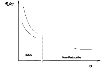
Figure 8: Expected shape of the short and long distance asymptotic behaviour of the function ${\cal R}(\sigma)$.

The problem of course is how to link the very short–distance regime (small $\sigma$) to the very long–distance (large $\sigma$) one. We shall be able to say a little bit more about that after the discussion of non–perturbative power corrections in the next section.

I wish to conclude this subsection with the discussion of an interesting model independent property of the ${\cal R}$–function [40]. It is the fact that, because of the positivity property of a spectral function $\frac{1}{\pi}\mbox{\rm Im}\Pi(t)\geq 0$, the function $-\log{\cal M}(\sigma)$ is a concave function of $\sigma$; or in other words, the slope of the function ${\cal R}(\sigma)$ must always be negative. This of course implies severe restrictions on the way that the two asymptotic regimes illustrated in Fig. 8 can be joined. The proof of this property is rather straightforward. It can be understood very simply by making an analogy with statistical mechanics: ${\cal R}(\sigma)$ can be viewed as the equilibrium “energy” $\langle t\rangle$ of a system with variable “energy” $t$ in thermal equilibrium with a second system at “temperature” $1/\sigma$. In this analogy, $\frac{1}{\pi}\mbox{\rm Im}\Pi(t)$ represents the “density of states” with “energy” $t$. Then the mean squared “energy fluctuation” is given by

$$-\frac{d}{d\sigma}{\cal R}(\sigma)\equiv\langle(t-\langle t\rangle)^{2}\rangle=\langle t^{2}\rangle-\langle t\rangle^{2}\geq 0,$$ (90)

which by definition is a positive quantity.

2 Gaussian Transform Sum Rules

The Gaussian transform of a spectral function

$${\cal G}(s,\tau)=\frac{1}{\sqrt{4\pi\tau}}\int_{0}^{\infty}dt\exp\left(-\frac{(s-t)^{2}}{4\tau}\right)\frac{1}{\pi}\mbox{\rm Im}\Pi(t),$$ (91)

can be evaluated in pQCD provided one keeps a finite width $\sqrt{2\tau}$ resolution in the gaussian kernel sufficiently large. These sum rules provide the framework to formulate quantitatively the notion of local duality. In the limit $\tau\rightarrow 0$ where the gaussian kernel becomes a delta function

$$\lim_{\tau\rightarrow 0}\frac{1}{\sqrt{4\pi\tau}}\exp\left(-\frac{(s-t)^{2}}{4\tau}\right)\Rightarrow\delta(s-t),$$ (92)

the Gaussian transform coincides with the spectral function itself

$$\lim_{\tau\rightarrow 0}{\cal G}(s,\tau)\Rightarrow\frac{1}{\pi}\mbox{\rm Im}\Pi(s).$$ (93)

There is in fact an interesting analogy between these sum rules and the theory of the “heat equation” [38]. The analogy is based on the observation that ${\cal G}(s,\tau)$ obeys the partial differential equation

$$\frac{\partial^{2}{\cal G}(s,\tau)}{(\partial s)^{2}}=\frac{\partial{\cal G}(s,\tau)}{\partial\tau},$$ (94)

which is the one dimensional heat equation if we interpret $s$ as a pseudo–“position” variable and $\tau$ as a pseudo–“time” variable. In this analogy, the hadronic spectral function corresponds to the initial “heat” (or “temperature”) distribution in a semi–infinite rod $0\leq s\leq\infty$ and ${\cal G}(s,\tau)$ measures the evolution in “time” $\tau$ of the “heat” distribution in this rod. The calculation of ${\cal G}(s,\tau)$ in pQCD is an expansion in powers of $\alpha_{s}(\sqrt{\tau})$ which blows up at small $\tau$–values; therefore, direct confrontation of the physical hadronic spectral function $\frac{1}{\pi}\mbox{\rm Im}\Pi(t)$ with pQCD cannot be made at small $\tau$–values. The confrontation can however be made at sufficiently large $\tau$–values by comparing the “evolved” physical hadronic spectral function ${\cal G}(s,\tau)$ with the corresponding pQCD theoretical prediction. The more we knew about non–perturbative corrections the smaller we should be able to go in “time” i.e. the smaller we would be able to take the width $\sqrt{2\tau}$ of the gaussian kernel and therefore the closer one could satisfy local duality.

Let us discuss how to get the Gaussian transform from a generic two–point function like $\Pi(q^{2})$ in eq. (37). First, one evaluates $\Pi(q^{2})$ at a complex point $q^{2}=s+i\Delta$ ($s$ and $\Delta$ are real positive variables) and at its complex conjugate $q^{2}=s-i\Delta$ (see Fig. 9)

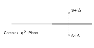
Figure 9: Points in the complex $q^{2}$–plane where the two–point function in eq. (95) is evaluated.

and defines the combination, (I am assuming for simplicity that the dispersion relation for $\Pi(q^{2})$ requires at most one subtraction, but the argument can be easily generalized as in the case discussed for the Laplace transform.)

$$\frac{\Pi(s+i\Delta)}{i\Delta}+\frac{\Pi(s-i\Delta)}{-i\Delta}=\int_{0}^{\infty}dt\,\frac{1}{(t-s)^{2}+\Delta^{2}}\,\frac{1}{\pi}\mbox{\rm Im}(t).$$ (95)

The integral in the r.h.s. brings in the convolution with a Lorentz–like kernel which we can write as a Laplace transform

$$\frac{1}{(t-s)^{2}+\Delta^{2}}=\int_{0}^{\infty}dx\,e^{-x\Delta^{2}}\,e^{-x(t-s)^{2}}.$$ (96)

Applying to this integral representation the techniques developed in the previous section 1 allows us to construct the inverse Laplace transform operator which is needed to obtain the Gaussian transform in eq. (91) from the Lorentz transform in eq. (95). It is the operator

$${\mbox{\bf L}}\equiv\lim_{N\rightarrow\infty}\,\lim_{\Delta^{2}\rightarrow\infty}\left|{}_{\frac{1}{N}\Delta^{2}=4\tau}\right.\,\frac{(-1)^{N}}{(N-1)!}\left(\Delta^{2}\right)^{N}\frac{\partial^{N}}{\left(\partial\Delta^{2}\right)^{N}}.$$ (97)

We then have the desired relation

$$\begin{split}\frac{1}{\sqrt{4\pi\tau}}&2\tau{\mbox{\bf L}}\left[\frac{\Pi(s+i\Delta)}{i\Delta}+\frac{\Pi(s-i\Delta)}{-i\Delta}\right]\\ &\Rightarrow\frac{1}{\sqrt{4\pi\tau}}\int_{0}^{\infty}dt\exp\left(-\frac{(s-t)^{2}}{4\tau}\right)\frac{1}{\pi}\mbox{\rm Im}\Pi(t).\end{split}$$ (98)

I will later come back to the physics of Gaussian sum rules, but I need first to introduce some properties of finite energy sum rules which is the subject of the next section.

3 Finite Energy Sum Rules

The moments of spectral functions

$${\cal M}_{n}(s)=\int_{0}^{s_{0}}dt\,t^{n}\,\frac{1}{\pi}\mbox{\rm Im}\Pi(t),$$ (99)

with $n=0,1,2,\cdots$ are also calculable quantities in QCD, provided that the upper limit $s_{0}$ is sufficiently large. Finite energy sum rules follow from the analyticity properties of two–point functions already discussed in section 3. Applying Cauchy’s integral formula to the contour in the complex $q^{2}$–plane shown in Fig. 10

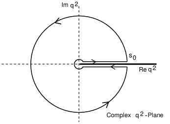
Figure 10: Contour of integration in the complex $q^{2}$–plane.

avoids the cut in the real axis and therefore results in

$$\frac{1}{2\pi i}\oint dq^{2}\,(q^{2})^{n}\,\Pi(q^{2})=0.$$ (100)

We now separate this integral into two pieces: one is the contribution from the paths above and below the real axis which pick up the discontinuity of the $\Pi(q^{2})$ function along this axis, and hence its imaginary part; the other is the contribution to the integral over the circle of radius $s_{0}$ [One should also check that there is no contribution from the little circle around the origin. The behaviour of $\Pi(q^{2})$ at small $q^{2}$ is usually known from low–energy properties of the two–point function.]. These two contributions have to match, resulting in the equation

$$\int_{0}^{s_{0}}dt\,t^{n}\,\mbox{\rm Im}\Pi(t)=-\frac{1}{2\pi i}\oint_{|q^{2}|=s_{0}}dq^{2}\,q^{2n}\,\Pi(q^{2}).$$ (101)

The integral in the l.h.s. is obtained using hadronic data, or inserting an hadronic ansatz; the integral in the r.h.s. is done in pQCD integrating the running coupling constant dependence over the circle of radius $s_{0}$ and scaling the result at $\mu^{2}=s_{0}$. Non–perturbative $1/q^{2}$–power corrections can also contribute in general to the r.h.s. integral. In QCD, and with $d$ the asymptotic power behaviour of a given spectral function as defined in eq. (70), finite energy sum rules with $n+d\geq 1$ are particularly sensitive to non–perturbative power corrections. These corrections will be the subject of the next section.

In finite energy sum rules, the question of subtractions in the primitive two–point functions can be dealt with by an appropriate integration by parts. For example, if one subtraction in $\Pi(q^{2})$ is required as for example in the case of the Adler function discussed in section 4, and we want to compute a general moment integral over the the circle of radius $s_{0}$, we can use the identity ($f(q^{2})$ is assumed to be non–singular,)

$$\oint_{|q^{2}|=s_{0}}dq^{2}\,f(q^{2})\,\Pi(q^{2})=-\oint_{|q^{2}|=s_{0}}\frac{dq^{2}}{q^{2}}\left[F(q^{2})-F(s_{0})\right]q^{2}\frac{d\Pi(q^{2})}{dq^{2}},$$ (102)

with $F(z)=\int_{0}^{z}dw\,f(w)$. As one increases the $n$–power in a finite energy sum rule, one becomes more and more sensitive to the detailed high energy behaviour of the hadronic spectral function. In the QCD expression of the r.h.s., this is reflected by the appearence of higher and higher values of the coefficients in the perturbative series in $\alpha_{s}(s)$ and therefore worse convergence, as well as by the appearance of non–perturbative condensates of higher and higher dimension.

Finite energy sum rules provide a very useful way to do the correct matching between a given ansatz of the low–energy hadronic spectral function and the onset of the perturbative continuum. For example, in the case of the Adler function discussed in section 4, let us consider the simplest hadronic ansatz of a narrow low–energy ground state plus a continuum i.e. the ansatz in eq. (23) which we have already discussed in connection with the phenomenological study of the Weinberg sum rules:

$$\frac{1}{\pi}\mbox{\rm Im}\Pi_{\mbox{\scriptsize\rm I}=1}(t)=f_{\rho}^{2}M_{\rho}^{2}\delta(t-M_{\rho}^{2})+\frac{N_{c}}{16\pi^{2}}\frac{2}{3}\theta(t-s_{0})[1+\cdots].$$ (103)

In this case, the application of the finite energy sum rule in eq. (101) with $n=0$ and in the chiral limit where $m_{u}=m_{d}\rightarrow 0$ does not depend on non–perturbative condensates (because of the absence of gauge invariant operators of dimension $d=2$ in QCD,) and results in the following constraint among the parameters of the hadronic ansatz

$$f_{\rho}^{2}M_{\rho}^{2}=\frac{N_{c}}{24\pi^{2}}\,s_{0}[1+\cdots].$$ (104)

Numerically, using the experimental values of $f_{\rho}$ and $M_{\rho}$ in this equation results in a value for the onset of the perturbative continuum $s_{0}\simeq 1.8\,\mbox{\rm GeV}^{2}$ which is quite reasonable, in the sense that it is sufficiently large to trust pQCD [With gluonic corrections incorporated at the two loop level, the resulting $s_{0}$ is reduced to $s_{0}\simeq 1.6\,\mbox{\rm GeV}^{2}$.].

I can now comment on a very interesting connection between finite energy sum rules and the Gaussian sum rules we discussed in the previous subsection. It has been shown in a general way [38], that matching a given low–energy hadronic spectral function ansatz to the perturbative continuum via finite energy sum rules guarantees that the corresponding Gaussian transform at large widths has then the correct asymptotic behaviour predicted by pQCD. This is an important point in phenomenological applications and therefore I want to discuss it in some detail. Very often one finds in the literature rather “precise” QCD sum rule “predictions” of masses or couplings which, however, have been obtained by fixing the onset of the pQCD continuum in the hadronic spectral function at some value using some “good physical sense” criteria, or even forgetting altogether about the QCD continuum. You can check that, unfortunately, the Gaussian transform of these spectral functions do not evolve to the shape predicted by pQCD. In other words, parameterizations of spectral functions which are not correctly constrained by finite energy sum rules are not guaranteed to be globally dual to QCD and therefore should be avoided. Let us illustrate this with some pictures. Figure 11 shows the evolution in the pseudo–“time” variable $\tau$ of the Gaussian transform of the spectral function ansatz in eq. (103) with the onset of the continuum $s_{0}$ fixed by the finite energy sum rule in eq. (104).

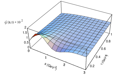
Figure 11: The Gaussian Transform of the Spectral Function in eq. (103) .

In the “heat evolution” analogy the spectral function in eq. (103) corresponds to the initial “heat distribution” in the $s$–axis. The picture shows the evolution in “time” of this “heat distribution” in the interval $0.1\,\mbox{\rm GeV}^{4}\leq\tau\leq 1\,\mbox{\rm GeV}^{4}$. We observe that asymptotically in “time”, i.e. for $\tau$ large, the spectral function evolves very well to the asymptotic “heat distribution” predicted by pQCD i.e.

$$\lim_{\tau\rightarrow\infty}{\cal G}(s,\tau)\Rightarrow\frac{1}{16\pi^{2}}\left(1-\mbox{\rm erf}(\frac{s}{2\sqrt{\tau}})\right)[1+\cdots],$$ (105)

where $\mbox{\rm erf}(x)$ denotes the error function $\mbox{\rm erf}(x)=\frac{2}{\sqrt{\pi}}\int_{0}^{x}dy\,e^{-y^{2}}$. By contrast, Fig. 12 shows the same evolution in the limit case of only a delta–function ansatz for the spectral function

$$\frac{1}{\pi}\mbox{\rm Im}\Pi_{\mbox{\scriptsize\rm I}=1}(t)=f_{\rho}^{2}M_{\rho}^{2}\delta(t-M_{\rho}^{2}),$$ (106)

with no continuum.

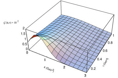
Figure 12: The Gaussian Transform of the Spectral Function in eq. (106) .

Clearly the corresponding asymptotic “heat distribution” fails to reproduce the shape predicted by pQCD. Global duality of a given hadronic spectral function ansatz with QCD is only obtained provided that the hadronic parameters are constrained to satisfy a system of finite energy sum rules equations.

5 Non–Perturbative Power Corrections

The physical vacuum of QCD is not the vacuum state which one uses in perturbation theory. Physical effects like spontaneous chiral symmetry breaking and/or confinement do not appear in an order by order perturbative treatment of QCD. A natural question to ask then is how are the pQCD results modified by non–perturbative effects at short–distances? This is the question which we shall be dealing with in this section. We shall see that non–perturbative effects in two–point functions evaluated at large $Q^{2}$–values appear as inverse power corrections in $Q^{2}$. They are the analogue of the higher twist corrections of deep inelastic scattering [2]. They can be systematically evaluated by doing Wilson’s operator product expansion [41] (OPE) in the physical vacuum. The power corrections appear then as the product of Wilson coefficients, which are calculable perturbatively, times universal non–zero vacuum expectation values of gauge invariant operators, the so called condensates which, although excluded by definition order by order in perturbation theory, they can a priori have non–zero values in the physical vacuum. Typical examples are the lowest dimension quark condensate $\langle\bar{\psi}\psi\rangle$ and gluon condensate $g_{\mbox{\rm{\scriptsize s}}}^{2}\langle\mbox{\rm tr}G_{\mu\nu}G^{\mu\nu}\rangle$. The operators which appear in any of the vacuum condensates which we shall be considering are assumed to be normal ordered.

1 Infrared Renormalon Ambiguities and Power Corrections

The need of non–perturbative power corrections to colour singlet gauge invariant two–point functions can be “hinted” from what emerges already in perturbation theory when summing a specific class of contributions. Let us consider the calculation of a typical two–point function, e.g. the Adler function which we have already defined in section 4, and let us restrict our attention to the class of Feynman diagrams generated by the replacement of a virtual gluon by one effective charge chain as shown in Fig 13.

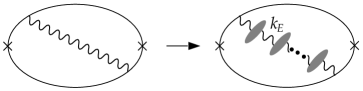
Figure 13: One of the Feynman diagrams which contributes to the Adler function with the gluon propagator replaced by an effective charge chain.

Formally, the chain of bubbles in Fig. 13 corresponds to the replacement of the ordinary free gluon propagator by the full gluon propagator–like function

$$\begin{split}&\frac{-i\left(g_{\mu\nu}-(1-\xi)\frac{k_{\mu}k_{\nu}}{k^{2}}\right)}{k^{2}+i\epsilon}(-ig_{s})^{2}\Rightarrow\\ &-i\left(g_{\mu\nu}-\frac{k_{\mu}k_{\nu}}{k^{2}}\right)\frac{4\pi\,\alpha_{\mbox{\small{\rm eff}}}(k_{E}^{2})}{k_{E}^{2}-i\epsilon}+i\xi\frac{k_{\mu}k_{\nu}}{k^{2}}\frac{(-ig_{s})^{2}}{k^{2}+i\epsilon},\end{split}$$ (107)

where $k_{E}$ denotes the euclidean virtual momentum carried by the chain; and $\xi$ is the usual covariant gauge parameter. The interesting quantity here is the effective charge function $\alpha_{\mbox{\small{\rm eff}}}(k_{E}^{2})$. The existence of an effective charge in non–abelian gauge theories with properties precisely analogous to those of the well known effective charge of QED is discussed in refs.[42, 43] and references therein. In terms of a characteristic scale, like e.g. the $\Lambda_{\overline{MS}}$ scale of the $\overline{MS}$–renormalization scheme,

$$\alpha_{\mbox{\small{\rm eff}}}(k_{E}^{2})=\frac{1}{\frac{-\beta_{1}}{2\pi}\log\frac{k_{E}^{2}}{c^{2}\Lambda_{\overline{MS}}^{2}}},$$ (108)

where

$$\beta_{1}=\frac{-11}{6}N_{c}+\frac{1}{3}n_{f}\qquad\mbox{\rm and}\qquad c^{2}=\exp\left\{\frac{67N_{c}-10n_{f}}{33N_{c}-6n_{f}}\right\}\,.$$ (109)

The $\beta_{1}$ factor is precisely the first coefficient of the QCD $\beta$–function. The effective charge encodes therefore the physics of the $\beta$–function; in particular the scale breaking property. Since, eventually, we are interested in the appearance of physical scales in QCD, it seems natural to focus our attention on the properties of those diagrams of perturbation theory generated by the insertion of effective charge–exchanges. Of course, we do that at the simplest level of keeping only the one loop dependence of the $\beta$–function. As far as one is only interested in general qualitative features this should not be a serious limitation. It is helpful now to look at the $Q^{2}$–$k_{E}^{2}$ plot in Fig. 14, where $k_{E}$ denotes the euclidean energy–momentum carried by the chain in Fig. 13.

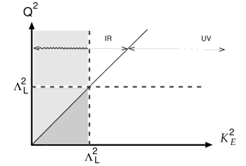
Figure 14: Integration regions of the virtual euclidean momentum $k_{E}^{2}$ for a fixed euclidean external momenta $Q^{2}$.

We shall refer to the integration regions $0\leq k_{E}^{2}\leq Q^{2}$ and $Q^{2}\leq k_{E}^{2}\leq\infty$ shown in Fig. 14 as the IR–region and the UV–region respectively. It is this IR–region of integration which is at the origin of the appearance of singularities, the so called IR renormalons, when tree level gluon propagators are replaced by the full summation of perturbation theory diagrams which define a renormalon chain as illustrated in Fig. 13. For reference, we also show in the plot in Fig. 14 the lines $Q^{2}=\Lambda_{L}^{2}$ and $k_{E}^{2}=\Lambda_{L}^{2}$, with $\Lambda_{L}=c\times\Lambda_{\overline{MS}}\simeq 1\,\mbox{\rm GeV}$ the Landau scale at which the pQCD effective charge becomes singular. In pQCD calculations, the external euclidean momenta is always chosen to be $Q^{2}\gg\Lambda_{L}^{2}$; however, regardless of how large $Q^{2}$ is taken, there will always be a region in the virtual $k_{E}^{2}$ integration which is below $\Lambda_{L}^{2}$ where pQCD is not defined. It is precisely this region of integration which, as we shall see in the next paragraph, leads to IR renormalon poles in the so called Borel plane. The appearance of these singularities is welcome because they reflect the limitations of perturbation theory and indicate the presence of non–perturbative power corrections, as indeed the OPE in the physical vacuum suggests [The reader may be curious to know about the fate of the UV renormalons in QCD. Ref. [51] and the references therein discuss this interesting topic.].

The leading contribution to the self–energy function $\Pi_{\mbox{\scriptsize\rm I}=1}(q^{2})$ in eq. (73) from the chain exchange diagrams in Fig.13 in the IR domain of integration $0\leq k_{E}^{2}\leq Q^{2}$ can be easily obtained and it has the following form $\left(C_{\rm F}=\frac{N_{c}^{2}-1}{2N_{c}}\right)$

$$\Pi_{\mbox{\scriptsize\rm I}=1}(Q^{2})\Rightarrow\frac{N_{c}}{32\pi^{2}}C_{\rm F}\int_{0}^{Q^{2}}dk_{E}^{2}\frac{k_{E}^{2}}{Q^{2}}\alpha_{\mbox{\small{\rm eff}}}(k_{E}^{2}).$$ (110)

Making the change of variables

$$w/2=-b_{0}\alpha(Q^{2})\log k_{E}^{2}/Q^{2}\,,\qquad\mbox{\rm where}\qquad b_{0}\equiv-\beta_{1}/2\pi$$ (111)

in the previous equation, one obtains

$$\Pi_{\mbox{\scriptsize\rm I}=1}(Q^{2})|_{\mbox{\small{\rm IR}}}=\frac{N_{c}}{16\pi^{2}}\,C_{\rm F}\,\frac{1}{2\pi b_{0}}\int_{0}^{\infty}dw\,e^{-\frac{w}{b_{0}\alpha(\mu^{2})}}\>\frac{1}{2-w}\left(\frac{Q^{2}}{\mu^{2}}\right)^{-w},$$ (112)

which leads to a contribution to the Adler function

$${\cal A}(Q^{2})|_{\mbox{\small{\rm IR}}}=\frac{N_{c}}{16\pi^{2}}\,C_{F}\,\frac{1}{2\pi b_{0}}\int_{0}^{\infty}dw\,e^{-\frac{w}{b_{0}\alpha(\mu^{2})}}\>\frac{w}{2-w}\left(\frac{Q^{2}}{\mu^{2}}\right)^{-w}.$$ (113)

This expression is already in the form of a Borel transform. An expansion around $w=0$ would generate the characteristic $n!$ behaviour of the perturbative expansion in $\alpha(\mu^{2})$ indicating that the corresponding series is not Borel summable. As already discussed by other authors [44, 45, 46], we find that the leading IR renormalon contribution to the Adler function appears as a pole in the Borel plane at the location $w=2$. There is no term in the IR expansion of the domain of integration which leads to a pole at $w=1$. From the previous change of variables one also sees that low values of $w$ are associated with momenta around the large scale $Q^{2}$, where perturbation theory is expected to give a good description of the dynamics. However, as $w$ goes up (and it has to go all the way up to infinity) one enters deeper and deeper into the IR region, where perturbation theory must fail or else QCD would not describe the spectrum of hadronic bound states that are observed. The singularity at $w=2$ exhibits this in its crudest form. More precisely, this singularity implies an ambiguity in the perturbative evaluation of the Adler function. Therefore, the analytic continuation in $w$ in eq. (113), or equivalently the resummation of perturbation theory into the effective charge $\alpha_{\mbox{\rm eff}}(k_{E}^{2})$ of eq. (108), that one has tried in order to obtain the full solution has failed. The ambiguity is encoded in the unavoidable prescription to skip the pole; and is of the form $\sim e^{-1/b_{0}\alpha(Q)}$ :

$$\Delta\Pi(Q^{2})|_{\mbox{\small{\rm IR}}}\sim\frac{N_{c}}{16\pi^{2}}\,\frac{6}{11}\,\frac{N_{c}^{2}-1}{N_{c}^{2}-2n_{f}}\left(\frac{\Lambda_{L}}{Q}\right)^{4},$$ (114)

i.e., an ambiguity which has the same $\frac{1}{Q^{4}}$ pattern as the gluon condensate contribution which appears in the OPE evaluation of the Adler function [47, 48, 49, 50]. Since the Adler function must be an unambiguous physical observable, there must exist another contribution that cancels the one in eq. (114). In other words, (Borel) resummed perturbation theory is requiring the presence of the gluon condensate (which is also ambiguous for the same reason) to combine with the result of eq. (113) and yield a final well–defined answer [44]. This is an example of how all–orders perturbation theory is capable of “hinting” at nonperturbative dynamics.

2 The ITEP Power Corrections

The intuitive physical picture which lies behind the non–perturbative power corrections introduced by the ITEP group [37] can be understood as follows. In terms of Feynman diagrams, the configurations which are sensitive to the IR-region are those where the hard external momentum $Q$ flows into the diagram and goes along the quark loop with very little transfer to the gluon propagator, or the one–renormalon chain. The gluon propagator is then in a non–perturbative regime where many soft gluon interactions are possible since the coupling constant in this regime is very large. The idea of the OPE is to factor out the hard part of the $Q$–flow and calculate it perturbatively, while collecting the bulk of the soft non–perturbative gluon interactions in a condensate of gluons which will be treated as a phenomenological parameter. In practice, the calculations in the OPE are performed by integrating the fermion loop in the presence of “background” gluon fields, including hard perturbative gluonic corrections if necessary [Ref.[52] gives a lot of technical details on how to do these calculations.]. The average of all possible gauge invariant configurations of “background” gluon fields defines then the condensates. Background fields in an ordinary Feynman diagram are indicated by terminating dots, like in Fig. 15.

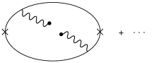
Figure 15: Feynman diagram representation of gluon condensate contributions.

The dots are a short–hand notation for the non–perturbative average over soft interactions. The perturbative evaluation of the “hard” part of the loop gives the corresponding Wilson coefficient and the net result is a contribution of the type ${\cal C}_{GG}\frac{g_{\mbox{\rm{\scriptsize s}}}^{2}\langle G_{a}^{\mu\nu}G^{a}_{\mu\nu}\rangle}{Q^{4}}$, where ${\cal C}_{GG}$ denotes the Wilson coefficient. The Wilson coefficient depends on the specific two–point function one is calculating, while the gluon condensate $g_{\mbox{\rm{\scriptsize s}}}^{2}\langle G_{a}^{\mu\nu}G^{a}_{\mu\nu}\rangle$ is treated as a universal phenomenological parameter. For example, in the case of the Adler function discussed in section 4 the gluon condensate gives a correction to the perturbative result in eq. (76):

$${\cal A}(Q^{2})|_{GG}=\frac{1}{12}\frac{\alpha_{\mbox{\rm{\scriptsize s}}}}{\pi}\frac{\langle G_{a}^{\mu\nu}G^{a}_{\mu\nu}\rangle}{Q^{4}}.$$ (115)

For two–point functions with composite operators of light quarks, there are also $1/Q^{4}$–corrections induced by the quark condensate, as illustrated in Fig. 16 below

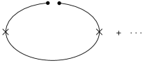
Figure 16: Feynman diagram representation of quark condensate contributions.

which give contributions of the type ${\cal C}_{{\bar{\psi}}\psi}\frac{m\langle{\bar{\psi}}_{L}\psi_{R}+{\bar{\psi}}_{R}\psi_{L}\rangle}{Q^{4}}$, where, as before, the Wilson coefficient ${\cal C}_{{\bar{\psi}}\psi}$ depends on the specific current operator. The appearance of a mass factor in front of the quark condensate is due to the conservation of chirality. In the case of the Adler function discussed in section 4 the quark condensate gives a correction to the perturbative result in eq. (76):

$${\cal A}(Q^{2})|_{{\bar{\psi}}\psi}=\frac{m_{u}\langle{\bar{u}}u\rangle+m_{d}\langle{\bar{d}}d\rangle}{Q^{4}}.$$ (116)

Higher order terms in the OPE bring in contributions from condensates of higher and higher dimension. Three new types of condensates appear at ${\cal O}(1/Q^{6})$: the quark gluon mixed condensate illustrated in Fig. 17 below

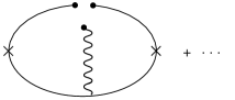
Figure 17: Feynman diagram representation of contributions from the mixed quark gluon condensate.

which brings contributions of the type ${\cal C}_{{\bar{\psi}}\psi}\frac{mg_{\mbox{\rm{\scriptsize s}}}\langle{\bar{\psi}}_{L}\sigma^{\mu\nu}\lambda^{(a)}\psi_{R}G_{\mu\nu}^{(a)}\rangle}{Q^{6}}$; the three gluon condensate illustrated in Fig. 18

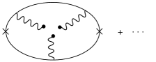
Figure 18: Feynman diagram representation of contributions from the three gluon condensate.

which can give contributions like ${\cal C}_{GGG}\frac{\langle g_{\mbox{\rm{\scriptsize s}}}^{3}G_{\mu\nu}^{(a)}G^{(b)\nu}_{\;\rho}G^{(b)\rho\mu}\rangle}{Q^{6}}$; and the four quark condensate illustrated in Fig. 19

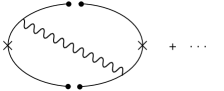
Figure 19: Feynman diagram representation of contributions from the four quark condensate.

which contributes to terms like ${\cal C}_{{\bar{\psi}}\psi{\bar{\psi}}\psi}\frac{\langle{\bar{\psi}}\Gamma\psi{\bar{\psi}}\Gamma\psi\rangle}{Q^{6}}$. In the case of the Adler function discussed in section 4 the quark gluon mixed condensate is suppressed by $\frac{m^{2}}{Q^{2}}$ factors. It has been shown [53, 54] that the three gluon condensate, without extra hard gluon corrections, gives no contribution to the Adler function. The four quark condensate contribution was first calculated in ref.[37] and it gives a correction to the perturbative result in eq. (76):

$$\begin{split}{\cal A}(Q^{2})_{{\bar{\psi}}\psi{\bar{\psi}}\psi}&=\left[-\frac{3}{2}\left\langle\left({\bar{u}}\gamma_{\mu}\gamma_{5}\lambda^{a}u-{\bar{d}}\gamma_{\mu}\gamma_{5}\lambda^{a}d\right)^{2}\right\rangle\right.\\ &-\left.\frac{1}{3}\left\langle\left({\bar{u}}\gamma_{\mu}\lambda^{a}u+{\bar{d}}\gamma_{\mu}\lambda^{a}d\right)\sum_{q=u,d,s}{\bar{q}}\gamma^{\mu}\lambda^{a}q\right\rangle\right]\frac{\pi\alpha_{\mbox{\rm{\scriptsize s}}}}{Q^{6}}.\end{split}$$ (117)

To leading order in the $1/N_{c}$–expansion these four quark condensates factorize into products of the lowest dimension quark condensate.

The phenomenological determinations of the gluon condensate and the quark condensate have still rather big errors. A generous range for the gluon condensate which covers most of the determinations is

$$\langle\alpha_{\mbox{\rm{\scriptsize s}}}G_{a}^{\mu\nu}G^{a}_{\mu\nu}\rangle=(0.08\pm 0.04)\,\mbox{\rm GeV}^{4}.$$ (118)

The quark condensate is scale dependent. The values obtained from a variety of sum rules are within the range

$$\frac{\langle\bar{u}u+\bar{d}d\rangle(1\,\mbox{\rm GeV}^{2})}{2}=-(0.013\pm 0.004)\,\mbox{\rm GeV}^{3}.$$ (119)

It turns out that with those values for the lower dimension condensates, the contribution from the leading non–perturbative power corrections in most of the sum rule applications -at the $Q^{2}$ values where one can trust the pQCD contributions- turn out to be already relatively small. This is due to the fact that the scale of perturbation theory $\Lambda_{\overline{MS}}$ is rather large; therefore, in order to get a convergent series in $\alpha_{\mbox{\rm{\scriptsize s}}}(Q^{2})$ one is obliged to go to rather high values of $Q^{2}$ where the power corrections are already quite small.

3 The Weinberg Sum Rules in the Light of the OPE

We are now in the position to understand why it is that the Weinberg sum rules we discussed in section 3 are satisfied in QCD. For this it is sufficient to consider the OPE applied to the two–point function $\Pi_{LR}(q)$ defined in eq. (12) [Notice that the OPE of this self–energy function is free from renormalon ambiguities, because in perturbation theory it is protected by chiral symmetry, which ensures that $\Pi_{LR}(Q^{2})=0$ order by order in powers of $\alpha_{s}$.]. Since this two–point function is chirally symmetric when quark masses are set to zero, the only possible inverse powers of $Q^{2}$ which can appear are those modulated by local order parameters of S$\chi$SB. In QCD there are no local order parameters of dimensions $d=2$ and $d=4$. Notice that $\langle\bar{\psi}\psi\rangle$, which has dimensions $d=3$ contributes to $\frac{1}{Q^{4}}$–terms but it appears multiplied by a quark mass factor; and therefore it disappears in the chiral limit. The first possible contribution comes from local order parameters of dimension $d=6$, i.e. the four–quark condensate contributions of the type illustrated in Fig. 18. The specific contribution to $\Pi_{LR}(Q^{2})$ has been calculated in ref. [37]. Their result is particularly simple in the large–$N_{c}$ limit where the vacuum expectation value of four–quark operators factorizes in a product of $\langle\bar{\psi}\psi\rangle$ terms, and therefore we have that

$$\lim_{Q^{2}\rightarrow\infty}\Pi_{LR}(Q^{2})=\frac{1}{Q^{6}}\left[-4\pi^{2}\left(\frac{\alpha_{s}}{\pi}+{\cal O}(\alpha_{s}^{2})\right)\langle\bar{\psi}\psi\rangle^{2}\right]+{\cal O}\left(\frac{1}{Q^{8}}\right)\,.$$ (120)

From this follow the two constraints in eqs. (18) and (19), and hence the two Weinberg sum rules in eqs. (15) and (16).

We also observe that the $\Pi_{LR}(Q^{2})$ expression in eq. (33) which results from the resonance dominance ansatz for the vector and axial–vector spectral functions has the required $\frac{1}{Q^{6}}$ behaviour at large–$Q^{2}$

$$\lim_{Q^{2}\rightarrow\infty}\Pi_{LR}(Q^{2})=\left(f_{V}^{2}M_{V}^{6}-f_{A}^{2}M_{A}^{6}\right)\frac{1}{Q^{6}}+{\cal O}(\frac{1}{Q^{8}}).$$ (121)

This is not surprising since the ansatz in question is nothing but a specific choice compatible with the spectrum predicted by QCD in the large–$N_{c}$ limit.

In section 3 I stressed the fact that it was not enough to know the the very low $Q^{2}$ behaviour of $\Pi_{LR}(Q^{2})$ in order to calculate the integral in eq. (32) which gives the electromagnetic $\pi^{+}-\pi^{0}$ mass difference. We now observe that it is not enough either to know only the very high $Q^{2}$ behaviour of the same function. The $\frac{1}{Q^{6}}$ behaviour of the short–distance OPE in eq. (120) cannot be extrapolated to the infrared region of the integral since it would lead to a divergent result as well. The simple resonance dominance ansatz in eq. (33) provides however, in this case, a correct matching of short–distance behaviour with the long–distance behaviour.

6 Some Examples of QCD Sum Rules

Here we shall discuss two applications of the techniques about sum rules in QCD developed in the previous sections. From a phenomenological point of view, the most striking application is the determination of the QCD coupling constant $\alpha_{\mbox{\rm{\scriptsize s}}}(m_{\tau}^{2})$ which has been made using the LEP data on hadronic tau decays. Another recent application uses very general properties of QCD sum rules to set lower bounds on the light quark masses.

1 Determination of the QCD Coupling Constant from Tau decays

Hadronic tau decays are governed by the spectral function associated with the charged current $L^{\mu}(x)=\bar{u}(x)\gamma^{\mu}\frac{1}{2}(1-\gamma_{5})d_{\theta}(x)$, where $d_{\theta}$ denotes the Cabibbo rotated $d$–quark. From the QCD point of view, the relevant two–point function is then

$$\begin{split}\Pi_{LL}^{\mu\nu}(q)&=4i\int d^{4}x\,e^{iq\cdot x}\langle 0|\mbox{\rm T}\left(L^{\mu}(x)L^{\nu}(0)^{\dagger}\right)|0\rangle\\ &=(q^{\mu}q^{\nu}-g^{\mu\nu}q^{2})\Pi_{LL}^{(1)}(Q^{2})+q^{\mu}q^{\nu}\Pi_{LL}^{(0)}(Q^{2}),\end{split}$$ (122)

which in full generality, when the quark masses are not neglected has two invariant functions corresponding to physical states with total angular momentum $J=1$ and $J=0$. From the phenomenological point of view, the quantity which is accessible to experimental determination is the hadronic tau decay branching ratio

$$\begin{split}R_{\tau}&\equiv\frac{\Gamma(\tau\rightarrow\nu_{\tau}+\mbox{\rm hadrons})}{\Gamma(\tau^{-}\rightarrow\nu_{\tau}e^{-}\bar{\nu}_{e})}=12\pi\times\\ &\int_{0}^{m_{\tau}^{2}}\frac{dt}{m_{\tau}^{2}}\left(1-\frac{t}{m_{\tau}^{2}}\right)^{2}\left\{\left(1+2\frac{t}{m_{\tau}^{2}}\right)\mbox{\rm Im}\Pi_{LL}^{(1)}(t)+\mbox{\rm Im}\Pi_{LL}^{(0)}(t)\right\}.\end{split}$$ (123)

The basic idea to apply here is the one we explained in the section 3 on finite energy sum rules, i.e. to confront the experimental determination of $R_{\tau}$ with the corresponding theoretical result [55] obtained from the contour integral in the complex $q^{2}$–plane shown in Fig. 10 with $s_{0}=m_{\tau}^{2}$:

$$\begin{split}R_{\tau}=6\pi i\times\oint_{|q^{2}|=m_{\tau}^{2}}&\frac{dq^{2}}{m_{\tau}^{2}}\left(1-\frac{q^{2}}{m_{\tau}^{2}}\right)^{2}\\ &\times\left\{\left(1+2\frac{q^{2}}{m_{\tau}^{2}}\right)\Pi_{LL}^{(1)}(q^{2})+\Pi_{LL}^{(0)}(q^{2})\right\}.\end{split}$$ (124)

The analyticity properties of the two–point function in eq. (122) imply that the r.h.s.’s of eqs. (123) and (124) should be equal. Notice that the evaluation of this integral only requires the knowledge of the invariant functions $\Pi_{LL}^{(1)}(q^{2})$ and $\Pi_{LL}^{(0)}(q^{2})$ in the complex big circle of radius $|q^{2}|=m_{\tau}^{2}$ and $m_{\tau}\simeq 1.78\,\mbox{\rm GeV}$ is a reasonably large scale to apply pQCD. Non–perturbative power corrections to this integral bring inverse powers of $m_{\tau}^{2}$. In fact, one of the nice features about this integral is that because of the combination of $q^{2}$–powers in the phase space factor which modulate the $\Pi_{LL}(q^{2})$’s functions in the integrand, the leading $1/m_{\tau}^{4}$ non–perturbative power corrections are suppressed up to terms of ${\cal O}\left[\left(\frac{\alpha_{\mbox{\rm{\scriptsize s}}}(m_{\tau}^{2})}{\pi}\right)^{2}\frac{\langle\alpha_{\mbox{\rm{\scriptsize s}}}GG\rangle}{m_{\tau}^{4}}\right]$. Also the contribution from the region in the circle near the real axis, where the validity of the OPE is perhaps questionable, is suppressed by the kinematic factor $\left(1-\frac{q^{2}}{m_{\tau}^{2}}\right)^{2}$. The result of the explicit calculation, which invokes quite a lot of refined techniques [56], can be written as follows

$$R_{\tau}=N_{c}\left(|V_{ud}|^{2}+|V_{us}|^{2}\right)^{2}S_{\mbox{\rm\footnotesize EW}}\left\{1+\delta^{{}^{\prime}}_{\mbox{\rm\footnotesize EW}}+\delta^{(0)}+\delta_{\mbox{\rm\footnotesize NP}}\right\},$$ (125)

where $S_{\mbox{\rm\footnotesize EW}}=1.0194$ and $\delta^{{}^{\prime}}_{\mbox{\rm\footnotesize EW}}=0.0010$ are the contributions from the leading and next–to–leading electroweak corrections, and

$$\begin{split}\delta^{(0)}=&\frac{\alpha_{\mbox{\rm{\scriptsize s}}}(m_{\tau}^{2})}{\pi}+5.2023\left(\frac{\alpha_{\mbox{\rm{\scriptsize s}}}(m_{\tau}^{2})}{\pi}\right)^{2}+26.366\left(\frac{\alpha_{\mbox{\rm{\scriptsize s}}}(m_{\tau}^{2})}{\pi}\right)^{3}\\ &+{\cal O}\left(\frac{\alpha_{\mbox{\rm{\scriptsize s}}}(m_{\tau}^{2})}{\pi}\right)^{4},\end{split}$$ (126)

is the result of the pQCD calculation in the chiral limit. The remaining factor $\delta_{\mbox{\rm\footnotesize NP}}\approx-0.016\pm 0.005$ includes the estimated effects of small quark mass–corrections and non–perturbative power corrections.

The most recent analysis, using the ALEPH data [57] gives the value

$$\alpha_{\mbox{\rm{\scriptsize s}}}(m_{\tau})=0.348\pm 0.008_{\mbox{\scriptsize exp}}\pm 0.015_{\mbox{\scriptsize th}}.$$ (127)

This value, when evolved with the renormalization group running to the $Z$–mass scale gives

$$\alpha_{\mbox{\rm{\scriptsize s}}}(M_{Z})=0.1211\pm 0.0008_{\mbox{\scriptsize exp}}\pm 0.0016_{\mbox{\scriptsize th}}\pm 0.0010_{\mbox{\scriptsize evol}},$$ (128)

which, with these errors, represents the most accurate determination of $\alpha_{\mbox{\rm{\scriptsize s}}}(M_{Z})$ from a single experiment .

2 Lower Bounds on the Light Quark Masses

The light $u$, $d$ and $s$ quarks in the QCD Lagrangian have bilinear couplings

$${\cal L}_{\mbox{\rm{\tiny QCD}}}={\cal L}_{\mbox{\rm{\tiny QCD}}}^{(0)}-\sum_{q=u,d,s}m_{q}{\bar{q}}(x)q(x)\,,$$ (129)

with masses $m_{q}\neq 0$ which explicitly break the chiral symmetry of the Lagrangian. The present situation concerning the values of the light quark masses in the $\overline{\mbox{\rm MS}}$ renormalization scheme, or any other scheme for that matter, has become rather confusing because of recent determinations of the light quark masses from lattice QCD [58, 59] which find substantially lower values than those previously obtained using a variety of QCD sum rules, (see e.g. refs. [60, 61, 62] and earlier references therein.) These new lattice determinations are also in disagreement with earlier lattice results [63]. More recently, an independent lattice QCD determination [64] using dynamical Wilson fermions finds results which, for $m_{u}+m_{d}$ are in agreement within errors with those of refs. [58, 59]; while for $m_{s}$ they agree rather well, again within errors, with the QCD sum rule determinations. [For a very lucid introduction to the techniques of Lattice QCD, see the lectures of M. Lüscher at this school [65].] Here, and as an application of the topics discussed in the previous sections, I shall show that there exist rigorous lower bounds on how small the light quark masses $m_{s}+m_{u}$ and $m_{d}+m_{u}$ can be [66]. There are two–point functions

$$\Psi(q^{2})\equiv i\int d^{4}xe^{iq\cdot x}\langle 0|T\left({\cal O}(x){\cal O}(0)^{\dagger}\right)|0\rangle,$$ (130)

with an appropriate choice of the local operator ${\cal O}(x)$ which are particularly sensitive to quark masses: the case where ${\cal O}$ is the divergence of the strangeness changing axial current

$${\cal O}(x)\equiv\partial_{\mu}A^{\mu}(x)=(m_{s}+m_{u}):\!\!{\bar{s}}(x)i\gamma_{5}u(x)\!\!:;$$ (131)

and another one where ${\cal O}$ is the scalar operator $S(x)$, defined as the isosinglet component of the mass term in the QCD Lagrangian

$${\cal O}(x)\equiv S(x)=\hat{m}[:\!\!{\bar{u}}(x)u(x)\!\!:+:\!\!{\bar{d}}(x)d(x)\!\!:],$$ (132)

with

$$\hat{m}\equiv\frac{1}{2}(m_{u}+m_{d}).$$ (133)

Both two–point functions obey dispersion relations which in QCD require two subtractions, and it is therefore appropriate to consider their second derivatives ($Q^{2}\equiv-q^{2}$):

$$\Psi^{\prime\prime}(Q^{2})=\int_{0}^{\infty}dt\frac{2}{(t+Q^{2})^{3}}\frac{1}{\pi}\mbox{\rm Im}\Psi(t).$$ (134)

The bounds follow from the restriction of the sum over all possible hadronic states which can contribute to the spectral function to the state(s) with the lowest invariant mass. It turns out that, for the two operators in (131) and (132), these hadronic contributions are well known phenomenologically; either from experiment or from chiral perturbation theory ($\chi$PT) calculations. On the QCD side of the dispersion relation, the two–point functions in question where the quark masses appear as an overall factor, are known in the deep euclidean region from pQCD at the four loop level. The leading non–perturbative $\frac{1}{Q^{2}}$–power corrections which appear in the operator product expansion when the time ordered product in (130) is evaluated in the physical vacuum [37] are also known. For the sake of simplicity, I shall only discuss here the case where ${\cal O}$ is the divergence of the strangeness changing axial current in eq. (131).

We shall call $\Psi_{5}(q^{2})$ the two–point function in (130) associated with the divergence of the strangeness changing axial current in (131). The lowest hadronic state which contributes to the corresponding spectral function is the $K$–pole. From eq. (134) we then have

$$\Psi_{5}^{\prime\prime}(Q^{2})=\frac{2}{(M_{K}^{2}+Q^{2})^{3}}2f_{K}^{2}M_{K}^{4}+\int_{t_{0}}^{\infty}dt\frac{2}{t+Q^{2})^{3}}\frac{1}{\pi}\mbox{Im}\Psi_{5}(t),$$ (135)

where $t_{0}=(M_{K}+2m_{\pi})^{2}$ is the threshold of the hadronic continuum.

It is convenient to introduce the moments $\Sigma_{N}(Q^{2})$ of the hadronic continuum integral

$$\Sigma_{N}(Q^{2})=\int_{t_{0}}^{\infty}dt\frac{2}{(t+Q^{2})^{3}}\times\left(\frac{t_{0}+Q^{2}}{t+Q^{2}}\right)^{N}\frac{1}{\pi}\mbox{\rm Im}\Psi_{5}(t).$$ (136)

One is then confronted with a typical moment problem (see e.g. ref. [67].) The positivity of the continuum spectral function $\frac{1}{\pi}\mbox{\rm Im}\Psi_{5}(t)$ constrains the moments $\Sigma_{N}(Q^{2})$ and hence the l.h.s. of (135) where the light quark masses appear. The most general constraints among the first three moments for $N=0,1,2$ are:

$$\Sigma_{0}(Q^{2})\geq 0,\quad\Sigma_{1}(Q^{2})\geq 0,\quad\Sigma_{2}(Q^{2})\geq 0;$$ (137)

$$\Sigma_{0}(Q^{2})-\Sigma_{1}(Q^{2})\geq 0,\quad\Sigma_{1}(Q^{2})-\Sigma_{2}(Q^{2})\geq 0;$$ (138)

$$\Sigma_{0}(Q^{2})\Sigma_{2}(Q^{2})-\left(\Sigma_{1}(Q^{2})\right)^{2}\geq 0\,.$$ (139)

The inequalities in eq. (138) are in fact trivial unless $2Q^{2}<t_{0}$, which constrains the region in $Q^{2}$ to too small values for pQCD to be applicable. The other inequalities lead however to interesting bounds which we next discuss.

The inequality $\Sigma_{0}(Q^{2})\geq 0$ results in a first bound on the running masses:

$$\begin{split}\left[m_{s}(Q^{2})+m_{u}(Q^{2})\right]^{2}\geq&\frac{16\pi^{2}}{N_{c}}\frac{2f_{K}^{2}M_{K}^{4}}{Q^{4}}\\ &\times\frac{1}{\left(1+\frac{M_{K}^{2}}{Q^{2}}\right)^{3}}\frac{1}{\left[1+\frac{11}{3}\frac{\alpha_{s}(Q^{2})}{\pi}+\cdots\right]},\end{split}$$ (140)

where the dots represent higher order terms which have been calculated up to ${\cal O}(\alpha_{s}^{3})$, as well as non–perturbative power corrections of ${\cal O}\left(\frac{1}{Q^{4}}\right)$ and strange quark mass corrections of ${\cal O}\left(\frac{m_{s}^{2}}{Q^{2}}\right)$ and ${\cal O}\left(\frac{m_{s}^{4}}{Q^{4}}\right)$ including ${\cal O}(\alpha_{s})$ terms . Notice that this bound is non–trivial in the large–$N_{c}$ limit ($f_{K}^{2}\sim{\cal O}(N_{c})$) and in the chiral limit ($m_{s}\sim M_{K}^{2}$). The bound is of course a function of the choice of the euclidean $Q$–value at which the r.h.s. in eq. (140) is evaluated. For the bound to be meaningful, the choice of $Q$ has to be made sufficiently large. In ref. [66] it is shown that $Q{\ \lower-1.2pt\vbox{\hbox{\hbox to0.0pt{$>$\hss}\lower 5.0pt\vbox{\hbox{$\sim$}}}}\ }1.4\>\mbox{\rm GeV}$ is already a safe choice to trust the pQCD corrections as such. The lower bound which follows from eq. (140) for $m_{u}+m_{s}$ at a renormalization scale $\mu^{2}=4\>\mbox{\rm GeV}^{2}$ results in the solid curves shown in Fig. 20 below.

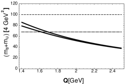
Figure 20: Lower bound in MeV for $[m_{s}+m_{u}](4\>\mbox{\rm GeV}^{2})$ versus $Q(\mbox{\rm GeV})$ from eq. (140).

These are the lower bounds obtained by letting $\Lambda^{(3)}_{\overline{MS}}$ vary [68] between 290 MeV (the upper curve) and 380 Mev (the lower curve). Values of the quark masses below the solid curves in Fig. 20 are forbidden by the bounds. For comparison, the horizontal lines in the figure correspond to the central values obtained by the authors of ref. [58]: their “quenched” result is the horizontal upper line; their “unquenched” result the horizontal lower line. It must be emphasized that in Fig. 20 one is comparing what is meant to be a “calculation” of the quark masses –the horizontal lines which are the lattice results of ref. [58]– with a bound which in fact can only be saturated in the limit where $\Sigma_{0}(Q^{2})=0$. Physically, this limit corresponds to the extreme case where the hadronic spectral function from the continuum of states is totally neglected! What the plots show is that, even in that extreme limit, and for values of $Q$ in the range $1.4\>\mbox{\rm GeV}{\ \lower-1.2pt\vbox{\hbox{\hbox to0.0pt{$<$\hss}\lower 5.0pt\vbox{\hbox{$\sim$}}}}\ }Q{\ \lower-1.2pt\vbox{\hbox{\hbox to0.0pt{$<$\hss}\lower 5.0pt\vbox{\hbox{$\sim$}}}}\ }1.6\>\mbox{\rm GeV}$ the “unquenched” lattice results of ref. [58] are already in difficulty with the bounds.

The quadratic inequality in (139) results in improved lower bounds for the quark masses which we show in Fig. 21 below.

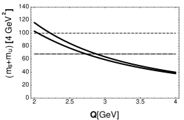
Figure 21: Lower bound in MeV for $[m_{s}+m_{u}](4\>\mbox{\rm GeV}^{2})$ from the quadratic inequality.

Like in Fig. 20, these are the lower bounds obtained by letting $\Lambda^{(3)}_{\overline{MS}}$ vary [68] between 290 MeV (the upper curve) and 380 Mev (the lower curve). Values of the quark masses below the solid curves in Fig. 21 are forbidden by the bounds. The horizontal lines in this figure are also the same lattice results as in Fig. 20.

The quadratic bound is saturated for a $\delta$–like spectral function representation of the hadronic continuum of states at an arbitrary position and with an arbitrary weight. This is certainly less restrictive than the extreme limit with the full hadronic continuum neglected, and it is therefore not surprising that the quadratic bound happens to be better than the ones from $\Sigma_{N}(Q^{2})$ for $N=0,1,$ and $2$. Notice however that the quadratic bound in Fig. 21 is plotted at higher $Q$–values than the bound in Fig. 20. This is due to the fact that the coefficients of the perturbative series in $\alpha_{\mbox{\rm{\scriptsize s}}}(Q^{2})$ become larger for the higher moments. In ref [66] it is shown that for the evaluation of the quadratic bound $Q{\ \lower-1.2pt\vbox{\hbox{\hbox to0.0pt{$>$\hss}\lower 5.0pt\vbox{\hbox{$\sim$}}}}\ }2\>\mbox{\rm GeV}$ is already a safe choice. One finds that in this case even the quenched lattice results of refs. [58, 59] are in difficulty with these bounds.

Similar bounds can be obtained for $m_{u}+m_{d}$ when one considers the two–point function associated with the divergence of the axial current

$$\partial_{\mu}A^{\mu}(x)=(m_{d}+m_{u}):\!\!{\bar{d}}(x)i\gamma_{5}u(x)\!\!:.$$ (141)

The method to derive the bounds is exactly the same as the one discussed above and therefore we only show, in Fig. 22 below, the results for the corresponding lower bounds which one obtains from the quadratic inequality.

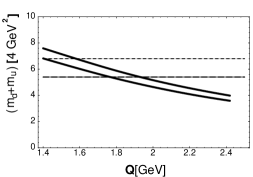
Figure 22: Lower bound in MeV for $[m_{d}+m_{u}](4\>\mbox{\rm GeV}^{2})$ from the quadratic inequality.

One finds again that the lattice QCD results of refs. [58, 59, 64] for $m_{u}+m_{d}$ are in serious difficulties with these bounds. The lower bounds discussed above are perfectly compatible with the sum rules results of refs. [60, 61, 62] and earlier references therein.

The two examples discussed in this section are rather illustrative of how sum rules can relate QCD short–distance calculations to low–energy hadronic experimental information. There are many other examples discussed in the literature. My hope is that these introductory lectures may help you to read the literature and to find new applications as well.

Acknowledgements

While preparing these lectures I have benefited a lot from the advice and help of my colleagues Santi Peris, Michel Perrottet and Joaquim Prades. It is a pleasure to thank them here. I also want to thank the students at the Les Houches summer school for their interest and active participation. They have been a very positive stimulus in producing this write–up.

References

- [1] A. Pich, Les Houches Lectures this volume.
- [2] A. Manohar, Les Houches Lectures this volume.
- [3] S. Narison, QCD Spectral Sum Rules, World Scientific 1989.
- [4] M.A. Shifman, Vacuum Structure and QCD Sum Rules, North-Holland, Amsterdam (1992).
- [5] S.D. Drell and A.C. Hearn, Phys. Rev. Lett. 16 (1966) 908.
- [6] M. Gell-Mann, M.L. Goldberger and W. Thirring, Phys. Rev. 95 (1954) 1612.
- [7] B.E. Lautrup, A. Peterman and E. de Rafael, Phys. Rep. 3C (1972) 193.
- [8] S.L. Adler, Phys. Rev. 140 (1965) B736.
- [9] W.I. Weisberger, Phys. Rev. 143 (1996) 1302.
- [10] M. Goldberger and S. Treiman, Phys. Rev. 110 (1958) 1178, 1478.
- [11] M. Gell-Mann and M. Lévy, Nuovo Cimento 16 (1960) 705.
- [12] S. Peris, Phys. Lett. B268 (1991) 415.
- [13] S. Peris, Phys. Rev. D46 (1992) 1202.
- [14] A. Manohar and H. Georgi, Nucl. Phys. B234 (1984) 189.
- [15] S. Peris and E. de Rafael, Phys. Lett. B309 (1993) 389.
- [16] S. Weinberg, Phys. Rev. Lett. 18 (1967) 507.
- [17] E.G. Floratos, S. Narison and E. de Rafael, Nucl. Phys. B155 (1979) 115.
- [18] K. Karabayashi and M. Suzuki, Phys. Rev. Lett. 16 (1966) 255.
- [19] Riazuddin and Fayyazuddin, Phys. Rev. 147 (1966) 1071.
- [20] G. Ecker, J. Gasser, H. Leutwyler, A. Pich, and E. de Rafael, Phys. Lett. B223 (1989) 425.
- [21] J. Gasser and H. Leutwyler, Ann. Phys. (N.Y.) 158 (1984) 142.
- [22] D. Treille, Les Houches lectures 1997 this volume.
- [23] S. Chivukula, Les Houches lectures 1997 this volume.
- [24] M. Knecht and E. de Rafael, hep-ph/9712457.
- [25] T. Das, G.S Guralnik, V.S. Mathur, F.E. Low and J.E. Young, Phys. Rev. Lett. 18 (1967) 759.
- [26] G. Ecker, J. Gasser, A. Pich and E. de Rafael, Nucl. Phys. B321 (1989) 311.
- [27] J. Bijnens and E. de Rafael, Phys. Lett. B273 (1991) 483.
- [28] M. Knecht and R. Urech, hep-ph/9709348, to appear in Nucl. Phys. B.
- [29] G. Källén, Helv. Phys. Acta 25 (1952) 417.
- [30] H. Lehmann, Nuovo Cimento 11 (1954) 342.
- [31] M. Veltman, DIAGRAMMATICA The Path to Feynman Diagrams, Cambridge Lecture Notes in Physics, 1994.
- [32] K.G. Chetyrkin, A.L. Kataev and F.V. Tkachov, Phys. Lett. B85 (1979) 277.
- [33] M. Dine and J. Sapirstein, Phys. Rev. Lett. 43 (1979) 668.
- [34] W. Celmaster and R.J. Gonsalves, Phys. Rev. Lett. 44 (1980) 560.
- [35] S.G. Gorishny, A.L. Kataev and S.A. Larin, Phys. Lett. B259 (1991) 144.
- [36] L.R. Surguladze and M.A. Samuel, Phys. Rev. Lett. 66 (1991) 560; 66 (1991) 2416 Erratum.
- [37] M.A. Shifman, A.I. Vainshtein and V.I. Zakharov, Nucl. Phys. B147 (1979) 385, 447.
- [38] R.A. Bertlmann, G. Launer and E. de Rafael, Nucl. Phys. B250 (1985) 61.
- [39] J.S. Bell and R. Bertlmann, Nucl. Phys. B177 (1981) 218; B187 (1981) 285.
- [40] E. de Rafael, Some Comments in QCD Sum Rules, in Phenomenology of Unified Theories, Dubrovnik 1983, Eds. H. Galić, B. Guberina and D. Tadić; World Scientific.
- [41] K.G. Wilson, Phys. Rev. 179 (1969) 1499.
- [42] N.J. Watson, Nucl. Phys. B494 (1997) 388.
- [43] J. Papavassiliou, E. de Rafael and N.J. Watson, Nucl. Phys. B503 (1997) 79.
- [44] A.H. Mueller, Nucl. Phys. B250 (1985) 327.
- [45] V.I. Zakharov, Nucl. Phys. B385 (1992) 452.
- [46] M. Beneke, Nucl. Phys. B405 (1993) 424.
- [47] F. David, Nucl. Phys. B209 (1982) 465.
- [48] F. David, Nucl. Phys. B234 (1984) 493.
- [49] V.A. Novikov, M.A. Shifman, A.I. Vainshtein and V.I. Zakharov, Phys. Reports 116 (1984) 105.
- [50] V.A. Novikov, M.A. Shifman, A.I. Vainshtein and V.I. Zakharov, Nucl. Phys. B249 (1985) 445.
- [51] S. Peris and E. de Rafael, Nucl. Phys. B500 (1997) 325.
- [52] V.A. Novikov, M.A. Shifman, A.I. Vainshtein and V.I. Zakharov, Fortsch. Phys. 32 (1984) 585.
- [53] M.S. Dubovikov and A.V. Smilga, Nucl. Phys. B185 (1981) 109.
- [54] W. Hubschmid and S. Mallik, Nucl. Phys. B207 (1982) 29.
- [55] E. Braaten, S. Narison and A. Pich, Nucl. Phys. B373 (1992) 581.
- [56] F. Le Diberder and A. Pich, Phys. Lett. B289 (1992) 165.
- [57] A. Höcker, “Mesure des fonctions spectrales du lepton et applications à la chromodynamique quantique”, Thesis, LAL 97-18 1997.
- [58] R. Gupta and T. Bhattacharya, Phys. Rev. D55 (1977) 7203.
- [59] B.J. Gough et al, preprint hep-ph/9610223.
- [60] J. Bijnens, J. Prades, and E. de Rafael, Phys. Lett. 348B (1995) 226.
- [61] M. Jamin and M. Münz, Z. Phys. C66 (1995) 633.
- [62] K.G. Chetyrkin, C.A. Dominguez, D. Pirjol and K. Schilcher, Phys. Rev. D51 (1995) 5090.
- [63] C.R. Allton et al, Nucl. Phys. B431 (1994) 667.
- [64] N. Eicker et al, SESAM–Collaboration, preprint hep-lat/9704019.
- [65] M. Lüscher, Les Houches Lectures this volume.
- [66] L. Lellouch, E. de Rafael and J. Taron, Phys. Lett. B414 (1997) 195.
- [67] N.I. Ahiezer and M. Krein, “Some Questions in the Theory of Moments”, Translations of Math. Monographs, Vol. 2; Amer. Math. Soc., Providence, Rhode Island (1962).
- [68] Review of Particle Properties, Phys. Rev. D54 (1996) 1.