Suppression of Bremsstrahlung and Pair Production due to Environmental Factors

Abstract

The environment in which bremsstrahlung and pair creation occurs can strongly affect cross sections for these processes. Because ultra-relativistic electromagnetic interactions involve very small longitudinal momentum transfers, the reactions occur gradually, spread over long distances. During this time, even relatively weak factors can accumulate enough to disrupt the interaction.

This review will discuss a variety of factors which can suppress bremsstrahlung and pair production, as well as related effects involving beamstrahlung and QCD processes. After surveying different theoretical approaches, experimental measurements will be covered. Recent accurate measurements by the SLAC E-146 collaboration will be highlighted, along with several recent theoretical works relating to the experiment.

(To appear in Reviews of Modern Physics)

Contents

toc

I Introduction

Bremsstrahlung and pair creation are two of the most common high energy electromagnetic processes, and the interaction cross sections are well known (Bethe and Heitler, 1934). However, it is much less well known that these cross sections can change dramatically depending on the environment in which the interaction occurs. The SLAC E-146 collaboration observed photon intensities as low as 1/4 of that predicted by Bethe and Heitler, and much larger suppression is possible.

The cross sections change because the kinematics of the processes dictates the interactions are spread over a significant distance, in contrast to the conventional picture where reactions occur at a single point. The momentum transfer between a highly relativistic interacting particle and the target nucleus can be small, especially along the direction of particle motion. When this longitudinal momentum transfer is small, the uncertainty principle dictates that the interaction is spread out over a distance, known as the formation length for particle production, or, more generally, as the coherence length.

If the medium in the neighborhood of the interaction has enough influence on the interacting particle during its passage through the formation zone, then the pair production or bremsstrahlung can be suppressed. When the formation length is long, weak but cumulative factors can be important. Some of the factors that may suppress electromagnetic radiation are multiple scattering, photon interactions with the medium (coherent forward Compton scattering), and magnetic fields. In crystals, where the atoms are arranged in ordered rows, a large variety of effects can suppress or enhance radiation.

The formation length has a number of interesting physical interpretations. It is the wavelength of the exchanged virtual photon. It is also the distance required for the final state particles to separate enough (by a Compton wavelength) that they act as separate particles. It is also the distance over which the amplitudes from several interactions can add coherently to the total cross section. All of these pictures can be helpful in understanding different aspects of suppression mechanisms.

The formation length was first considered by Ter-Mikaelian in 1952 (Feinberg, 1994). It occurs in both classical and quantum mechanical calculations. Classically, all electromagnetic processes have a phase factor

$$\Phi=\exp{\{i[\omega t-{\bf k}\cdot{\bf r}(t)]\}}$$ (1)

where $\omega$ is the photon frequency, $t$ is the time, ${\bf k}$ is the photon wave vector, and ${\bf r}(t)$ is the electron position. The formation length is the distance over which this phase factor maintains coherence; the electron and photon have slightly different velocities, which causes them to gradually separate. Coherence is maintained over a distance for which $\omega t-{\bf k}\cdot{\bf r}(t)\sim 1$. Around an isolated atom $\omega=|{\bf k}|c$, so, neglecting the (small) angle between ${\bf k}$ and ${\bf r}$, for a straight trajectory

$$l_{f0}={2E^{2}\over\omega m^{2}c^{3}}$$ (2)

where $E$ is the electron energy, $m$ is the electron mass, and $c$ the speed of light. The $f0$ subscript denotes the unsuppressed (free space) formation length. Electromagnetic interactions are spread over this distance. If $E$ is large and $\omega$ small, $l_{f0}$ can be very long. For example, for a 25 GeV electron radiating a 10 MeV bremsstrahlung photon, $l_{f0}=100\mu$m. This distance was the basis for the suppression calculations by Landau and Pomeranchuk, discussed in Sec. II.

The formation length also occurs in quantum mechanical calculations. Electron bremsstrahlung, where an electron interacts with a nucleus and emits a real photon is a good example. As the electron accelerates, part of its surrounding virtual photon field shakes loose. Neglecting the photon emission angle and electron scattering, the momentum transfer in the longitudinal ($+z$) direction is

$$q_{\parallel}=p_{e}-p_{e}^{\prime}-p_{\gamma}=\ \sqrt{(E/c)^{2}\ -\ (mc)^{2}}-\sqrt{((E-k)/c)^{2}\ -\ (mc)^{2}}-k/c$$ (3)

where $p_{e}$ and $p_{e}^{\prime}$ are the electron momenta before and after the interaction respectively and the photon momentum $p_{\gamma}=k/c$, with $k=\hbar\omega=\hbar|{\bf k}|/c$ the photon energy. For $\gamma=E/mc^{2}\gg 1$ this simplifies to

$$q_{\parallel}\sim{m^{2}c^{3}k\over 2E(E-k)}.$$ (4)

Here, we have used the small $y$ approximation $\sqrt{1-y}\sim 1-y/2$. For high energy electrons emitting low energy photons, $q_{\parallel}$ can become very small. For the above example, $q_{\parallel}=0.002\$eV/c. Because $q_{\parallel}$ is so small, the uncertainty principle requires that the radiation must take place over a long distance:

$$l_{f0}={\hbar\over q_{\parallel}}={2\hbar E(E-k)\over m^{2}c^{3}k}.$$ (5)

For $k\ll E$, this matches Eq. (2); the momentum transfer approach is needed only for $k\sim E$.

This formation length appears in most electromagnetic processes including pair production, transition radiation, Čerenkov radiation and synchrotron radiation. Usually, $q_{\parallel}$ acquires additional terms to account for specific interactions with the target medium. This review will discuss a number of these additions, and show how they affect bremsstrahlung and pair production. Formation lengths also apply to processes involving other forces; this review will consider a few non-electromagnetic interactions, showing how kinematics can dictate that diverse reactions share many fundamental traits.

The formation length is the distance over which the interaction amplitudes can add coherently. So, if an external force doubles $q_{\parallel}$, thereby halving $l_{f}$, then the radiation intensity is also halved, from $\sim l_{f}^{2}$ to $\sim 2\cdot(l_{f}/2)^{2}$ as the trajectory splits into two independent emitting regions. If an electron traversing a distance $D$ radiates, the trajectory acts as $D/l_{f}$ independent emitters, each with a strength proportional to $|l_{f}|^{2}$, so the total radiation is proportional to $l_{f}$. As external factors increase $q_{\parallel}$ and reduce $l_{f}$, the radiation drops proportionally.

A similar coherence distance $\hbar/q_{\perp}$ limits the perpendicular distance over which coherent addition is possible. However, because $q_{\perp}\gg q_{\parallel}$, this distance is much smaller, and of lesser interest here.

This article begins by considering separate classical and quantum mechanical (semi-classical) calculations of suppression due to multiple scattering. Suppression due to photon interactions with the medium, pair creation and external magnetic fields will then be similarly considered.

Other calculations have considered the multiple scattering in more detail, as diffusion of the electron. Migdal’s 1956 calculation, in Sec. III, was the first; it has become something of a standard. A number of recent calculations of suppression are described in Secs. V to VII.

Experimental work is surveyed in Sec. IX, beginning with the first cosmic ray studies of Landau-Pomeranchuk-Migdal (LPM) suppression shortly after Migdal’s paper appeared. These suffered from very limited statistics, and hence had limited significance. In the 1970’s and 1980’s, a few accelerator experiments provided some data, but still with limited accuracy. In 1993, SLAC experiment E-146 made detailed measurements of suppression due to multiple scattering and photon-medium interactions. E-146 confirmed Migdal’s formula to good accuracy, and at least partly inspired the more recent calculations in Secs. V to VII; because of this timing, some reference will be made to E-146 before the experiment is described in detail.

Some more specialized topics will also be considered. Section X considers suppression in plasmas, where particles with similar energies interact with each other. Section XI shows how suppression mechanisms can affect electromagnetic showers, with a focus on cosmic ray air showers. Section XII surveys the application of LPM formalism to hadrons scattering inside nuclei, where color charge replaces electric charge, and gluons replace photons. Finally, a number of open questions will be presented.

Earlier reviews (Feinberg and Pomeranchuk, 1956) (Akhiezer and Shul’ga, 1987) and monographs (Ter-Mikaelian, 1972) (Akhiezer and Shul’ga, 1996) have discussed these topics. A recent article (Feinberg, 1994) discusses the subject’s early development.

Unless otherwise indicated, energies will be given in electron volts (eV) and momentum in eV/c; $\hbar c$ is $1.97\times 10^{-7}$eV m and the fine structure constant $\alpha=e^{2}/\hbar c\approx 1/137$, where $e$ is the electric charge. For both bremsstrahlung and pair conversion, $E$ will represent electron/positron energy and $k$ photon energy.

II Classical and Semi-classical Formulations

Landau and Pomeranchuk (1953a) used classical electromagnetism to demonstrate bremsstrahlung suppression due to multiple scattering; the suppression comes from the interference between photons emitted by different elements of electron pathlength. For those with quantum tastes, subsection II B gives a simple semi-classical derivation based on the uncertainty principle.

A Classical Bremsstrahlung - Landau and Pomeranchuk

The classical intensity for radiation from an accelerated charge in the influence of a nucleus with charge $Z$ is

$${d^{2}I\over d\omega d\Omega}={Z^{2}e^{2}\omega^{2}\over 4\pi^{2}c^{3}}\bigg{|}\int{\bf n}\times d{\bf r}\exp{\{i[(\omega t-{\bf k}\cdot{\bf r}(t)]\}}\bigg{|}^{2}$$ (6)

where $d{\bf r}={\bf v}(t)dt$, n is the photon direction and ${\bf v}(t)$ the electron velocity. The angular integration $d\Omega$ is over all possible photon and outgoing electron directions. The classical bremsstrahlung spectrum can be found by assuming that v changes abruptly during the collision. Then, the integral splits into two pieces and the emission is easily found:

$${d^{2}I\over d\omega d\Omega}={Z^{2}e^{2}\over 4\pi^{2}c}\bigg{|}{{\bf k}\times{\bf v_{1}}\over{\bf k}\cdot{\bf v_{1}}-|{\bf k}|c}-{{\bf k}\times{\bf v_{2}}\over{\bf k}\cdot{\bf v_{2}}-|{\bf k}|c}\bigg{|}^{2}.$$ (7)

where ${\bf v}_{1}$ and ${\bf v}_{2}$ are the electron velocity before and after the interaction respectively. With small angle approximations, ${\bf k}\cdot{\bf v}=\omega(1-1/2\gamma^{2})(1-\theta_{\gamma}^{2}/2)$, where $\theta_{\gamma}$ is the angle between the photon and incident electron direction and $|{\bf k}\times{\bf v}|=|{\bf k}||{\bf v}|\theta_{\gamma}$, the bremsstrahlung angular distribution may be derived (for $\gamma\gg 1,k\ll E$):

$${dI^{2}\over d\omega d\Omega}={Z^{2}e^{2}\gamma^{4}|{\bf\Delta v}|^{2}\over\pi^{2}c^{3}}{(1+\gamma^{4}\theta_{\gamma}^{4})\over(1+\gamma^{2}\theta_{\gamma}^{2})^{4}}$$ (8)

where ${\bf\Delta v}={\bf v}_{1}-{\bf v}_{2}$. The overall emission intensity can be found by integrating over $d\Omega$, and expressed in terms of the change in electron momentum $q=\gamma m|{\bf\Delta v}|$. Then,

$${dI\over d\omega}={2Z^{2}e^{2}q^{2}\over 3\pi m^{2}c^{3}}.$$ (9)

The complete bremsstrahlung cross section can be found by multiplying this by the elastic scattering cross section, as a function of $q$ and converting from classical field intensity to cross section (Jackson, 1975, pg. 709):

$${d\sigma\over dk}={16Z^{2}\alpha r_{e}^{2}\over 3k}\int_{q_{min}}^{q_{max}}{dq\over q}$$ (10)

where $r_{e}=e^{2}/mc^{2}=2.8\times 10^{-15}$ m is the classical electron radius. The integral evaluates to $\ln{(q_{max}/q_{min})}$, often called the form factor. This form factor is roughly equivalent to $\ln{(\theta_{max}/\theta_{min})}$, where $\theta$ is the electron scattering angle; this representation is convenient, because the distributions of angles depend on the suppression. The use of $\alpha$, and implicitly $\hbar$ is needed to convert from field intensity to number of photons.

The minimum and maximum momentum transfers correspond to maximum and minimum effective impact parameters respectively. For a bare nucleus, the minimum impact parameter is the electron Compton wavelength $\lambda_{e}=\hbar/mc=r_{e}/\alpha=3.8\times 10^{-13}$ m, so $q_{max}=2mc$. When the momentum transfer $q_{max}$ is larger than $2mc$, the electron scatters by an angle larger than $1/\gamma$. Then, coherence between the incoming and outgoing electron pathlength (implied in Eq. (7)) is lost and the cross section drops. The probability of such a large scatter is very small. This loss of coherence foreshadows how multiple scattering affects the electron trajectory and hence the radiation. The minimum momentum transfer occurs when $q_{\perp}=0$ and $q_{min}=q_{\parallel}$.

However, nuclei are generally surrounded by electrons which screen the nuclear charge. For ultrarelativistic electrons, screening is important over almost the entire range of $k$. Screening shields the radiating electron from the nucleus at large distances, so the maximum impact parameter is the Thomas-Fermi atomic radius $a=0.8Z^{-1/3}a_{0}$, for $Z\gg 1$ (Tsai, 1974), where the Bohr radius $a_{0}=\hbar/\alpha mc=r_{e}/\alpha^{2}=5.3\times 10^{-9}$ m. Then, $q_{min}=1.25\hbar/\alpha mcZ^{1/3}$ and $\ln{(q_{max}/q_{min})}=\ln{(2.5/\alpha Z^{-1/3})}$. A more detailed calculation finds $\ln{(184Z^{-1/3})}$ for the form factor (Bethe and Heitler, 1934).

This classical calculation is valid only for $y=k/E\ll 1$. A Born approximation quantum mechanical calculation gives a similar result, but covers the entire range of $y=k/E$ (Bethe and Heitler, 1934):

$${d\sigma_{BH}\over dk}={4\alpha r_{e}^{2}\over 3k}\bigg{(}y^{2}+2[1+(1-y)^{2}]\bigg{)}Z^{2}\ln{(184Z^{-1/3})}={1\over 3nX_{0}k}\bigg{(}y^{2}+2[1+(1-y)^{2}]\bigg{)}$$ (11)

where the radiation length

$$X_{0}=[4n\alpha r_{e}^{2}Z^{2}\ln{(184Z^{-1/3})}]^{-1},$$ (12)

with $n$ the number of atoms per unit volume. More sophisticated calculations, discussed in Section IV, include additional terms in the cross section and radiation length. With a more detailed screening calculation, a small constant may be subtracted from the form factor. However, Eq. (11) is a good semi-classical benchmark.

If the interaction occurs in a dense medium, however, this treatment may be inadequate. The interaction is actually spread over the distance $l_{f0}$; if the electron multiple scatters during this time, it can affect the emission. The multiple scattering changes the electron path, so that

$${\bf v}(t)={\bf v}_{z}(t)+{\bf v}_{\perp}(t)={\bf v}(0)(1-\theta_{MS}(t)^{2}/2)+|{\bf v}(0)|\theta_{MS}(t){\bf\Theta}$$ (13)

where $\bf\Theta$ is a unit vector perpendicular to the initial direction of motion and $\theta_{MS}(t)$ is the electron multiple scattering in the time interval 0 to $t$. The particle trajectory is then ${\bf r}(t)=\int{\bf v}(t)dt$, so that

$${\bf k}\cdot{\bf r}(t)=|{\bf v}(0)|\ |{\bf k}|(1-{\theta_{\gamma}^{2}\over 2})\int_{0}^{t}(1-{\theta_{MS}^{2}\over 2})dt+|{\bf k}|\theta_{\gamma}\cdot\int_{0}^{t}\theta_{MS}(t)dt$$ (14)

where $\theta_{\gamma}$ is the angle between the photon and the initial electron direction. Landau and Pomeranchuk took $\theta_{MS}^{2}=\langle\theta_{MS}^{2}\rangle$. Over a distance $d={\bf v}_{z}t$, the rms multiple scattering is (Rossi, 1952)

$$\langle\theta_{MS}^{2}\rangle=({E_{s}\over E})^{2}{d\over X_{0}}$$ (15)

where $X_{0}$ is the radiation length and $E_{s}=mc^{2}\sqrt{4\pi/\alpha}=21.2MeV$.

The effect of multiple scattering can be found by inserting the trajectory of Eq. (13) into Eq. (6). This calculation simplifies with a clever choice of coordinate system. If the origin is centered on the formation zone, with ${\bf v}_{\perp}=0$ at $z=0$, then the multiple scattering distributes evenly before and after the ‘interaction’. Then, ${\bf v}_{1}$ and ${\bf v}_{2}$ are equally affected by multiple scattering, with

$${\bf k}\cdot{\bf v}_{1}={\bf k}\cdot{\bf v}_{2}=|{\bf k}|(1-1/2\gamma^{2})(1-\theta_{\gamma}^{2}/2)(1-\theta_{MS/2}^{2}/2)$$ (16)

and

$$|{\bf k}\times{\bf v}_{1}|=|{\bf k}\times{\bf v}_{2}|=|{\bf k}|(1-1/2\gamma^{2})\sqrt{\theta_{\gamma}^{2}+\theta_{MS/2}^{2}},$$ (17)

where $\theta_{MS/2}$ is the multiple scattering in half of the formation length. The angular addition in Eq. (17) is in quadrature because the angles are randomly oriented in the plane perpendicular to the electron direction. If the multiple scattering occurs on the same time scale as the interaction, then Eq. (8) becomes

$${dI^{2}\over d\omega d\Omega}={Z^{2}e^{2}\gamma^{4}|{\bf\Delta v}|^{2}\over\pi^{2}c^{3}}{[1+\gamma^{4}(\theta_{\gamma}^{2}+\theta_{MS/2}^{2})^{2}]\over[1+\gamma^{2}(\theta_{\gamma}^{2}+\theta_{MS/2}^{2})]^{4}}$$ (18)

For $\theta_{MS/2}^{2}>1/\gamma^{2}+\theta_{\gamma}^{2}$, the radiation will be reduced and the angular distribution changed. If the multiple scattering in the formation zone is large enough, emission is suppressed. For $\theta_{\gamma}\ll 1/\gamma$, this happens when

$$\omega<{E_{s}^{2}E^{2}\over m^{4}c^{7}X_{0}}.$$ (19)

Photons with lower energies will be suppressed. Equation (18) also shows that the angular distributions will be affected. Because multiple scattering can reduce the coherence length, a more detailed calculation is required to find the degree of suppression. Landau and Pomeranchuk (1953b) started with the expression

$${dI\over d\omega}={Z^{2}e^{2}\omega^{2}\over 4\pi^{2}c^{3}}\int_{-\infty}^{\infty}({\bf n}\times d{\bf r}_{1})\cdot\int_{-\infty}^{\infty}({\bf n}\times d{\bf r}_{2})\int d{\bf n}\exp{\{i\omega[(t_{1}-t_{2})-{\bf n}\cdot({\bf r_{1}}-{\bf r_{2}})/c]\}},$$ (20)

which simplifies to

$${dI\over d\omega}={Z^{2}e^{2}\omega\over\pi c^{2}}\int_{-\infty}^{+\infty}dt_{1}\int_{-\infty}^{+\infty}dt_{2}{\exp{[i\omega(t_{1}-t_{2})]}\over|{\bf r}_{12}|}(J_{1}+J_{2})$$ (21)

where

$$J_{1}={\bf v}_{1}\cdot{\bf v}_{2}-{({\bf v}_{1}\cdot{\bf r}_{12})({\bf v}_{2}\cdot{\bf r}_{12})\over r_{12}^{2}}\bigg{(}\sin{(g)}+{3g\cos(g)-sin(g)\over g^{2}}\bigg{)}$$ (22)

and

$$J_{2}=(-2{\bf v}_{1}\cdot{\bf v}_{2})\bigg{(}{g\cos(g)-\sin(g)\over g^{2}}\bigg{)}.$$ (23)

Here $g=\omega|{\bf r}_{12}|/c$ and ${\bf r_{12}}={\bf r}(t_{1})-{\bf r}(t_{2})$. The $J_{1}$ term was evaluated by Landau and Pomeranchuk (1953b) while the $J_{2}$ term, neglected by Landau and Pomeranchuk was evaluated by Blankenbecler and Drell (1996), who found $J_{1}=J_{2}$. Landau and Pomeranchuk still found the ’right’ result, compensating by using a perpendicular momentum transfer due to multiple scattering twice the correct one.

These integrals can be evaluated by using the electron trajectory given in Eqs. (13) and (14). Landau and Pomeranchuk gave a formula for the total (summed over time) emission.

$${dI\over d\omega}={Z^{2}e^{2}\omega\over\pi c^{2}}\int_{-\infty}^{\infty}dT\int_{-\infty}^{\infty}{dt\over t^{3}}e^{i\omega t}\bigg{[}{\bigg{(}\int_{0}^{t}\theta_{MS}(t)dt\bigg{)}^{2}}-{t\theta_{MS}\int_{0}^{t}\theta_{MS}(t)dt}\bigg{]}\times$$ (24)

$$\sin{\bigg{[}\omega\bigg{(}{vt\over c}-{1\over 2}\int_{0}^{t}\theta_{MS}^{2}(t)dt+{1\over 2t}\big{(}\int_{0}^{t}\theta_{MS}dt\big{)}^{2}\bigg{)}\bigg{]}}$$ (25)

where the integral over $T=t_{1}-t_{2}$, will be factored out to get the emission per unit time. The remaining integral is evaluated by replacing the angular quantities by their average values. For example,

$$\langle\int_{0}^{t}\theta_{MS}(t)dt\rangle={E_{s}^{2}ct|t|\over 2E^{2}X_{0}}$$ (26)

Landau and Pomeranchuk expressed their results in emission per unit time. In terms of the more prevalent total emission,

$${dI\over d\omega}={4Z^{2}e^{2}\over 3c}\int_{0}^{\infty}dX\sin\big{(}X+{E^{2}E_{s}^{2}X^{2}\over 3m^{4}c^{7}\omega X_{0}}\big{)}$$ (27)

For $\omega\ll E_{s}^{2}c/E^{2}X_{0}$, the emission is

$${dI\over d\omega}=\sqrt{2\pi\over 3}{Z^{2}e^{2}m^{2}c^{3}\over E_{s}E}\sqrt{\omega X_{0}\over c}$$ (28)

In the strong suppression limit, the field intensity $dI/d\omega\sim\sqrt{\omega}$, compared to an isolated interaction, where $dI/d\omega$ is independent of $\omega$; the corresponding cross sections scale as $1/\sqrt{\omega}$ and $1/\omega$ respectively. The following subsection will describe a simple semi-classical derivation of the same result, and also discuss some of its implications.

B Bremsstrahlung - Quantum approach

Bremsstrahlung suppression due to multiple scattering can also be found by starting with Eq. (5). Multiple scattering can suppress bremsstrahlung if it contributes significantly to $q_{\parallel}$ (Feinberg and Pomeranchuk, 1956). Multiple scattering affects $q_{\parallel}$ by reducing the electron longitudinal velocity. For a rough calculation, the multiple scattering angle can be taken as the average scattering angle. As before, the multiple scattering is divided into two regions: before and after the interaction. The longitudinal momentum transfer from the nucleus is

$$q_{\parallel}=\sqrt{(E\cos{\theta_{MS/2}}/c)^{2}-(mc)^{2}}-\sqrt{[(E-k)\cos{\theta_{MS/2}}/c]^{2}-(mc)^{2}}-k/c$$ (29)

where $\theta_{MS/2}$ is the multiple scattering in half the formation length, $(E_{s}/E)\sqrt{l_{f}/2X_{0}}$. The post-interaction scattering is based on the outgoing electron energy $E-k$. The inclusion of electron energy loss is a significant advantage of the quantum formulation. With some small angle approximations,

$$q_{\parallel}={km^{2}c^{3}\over 2E(E-k)}+{k\theta_{MS/2}^{2}\over 2c}$$ (30)

Multiple scattering is significant if the second term is larger than the first. This happens if $\theta_{MS/2}>1/\gamma$, or for

$$k<k_{LPM}={E(E-k)\over E_{LPM}}$$ (31)

where $E_{LPM}$ is a material dependent constant, given by

$$E_{LPM}={m^{4}c^{7}X_{0}\over\hbar E_{s}^{2}}={m^{2}c^{3}X_{0}\alpha\over 4\pi\hbar}\approx 7.7\ {\rm TeV/cm}\cdot X_{0}.$$ (32)

Table I gives $E_{LPM}$ in a variety of materials. This definition of $E_{LPM}$ was used by Landau and Pomeranchuk (1953a), Galitsky and Gurevich (1964), Klein (1993) and others, but is twice that used in some papers (Anthony, 1995, 1997) (Baier, 1996), and $1/8$ of that in others (Stanev, 1982). The last choice is convenient for working with Migdal’s equations (Sec. III), but not for the semi-classical derivation.

For $k\ll E$, Eq. (31) matches the classical result: photon emission for $k<k_{LPM}=E^{2}/E_{LPM}$ is reduced. For example, for 25 GeV electrons in lead, photon emission below 125 MeV is suppressed. For higher energy electrons, a large portion of the spectrum can be suppressed. For 4.3 TeV electrons in lead, fewer photons with $k<2.15$ TeV are radiated. At the endpoint of the spectrum, $k\rightarrow E$, $l_{f0}$ approaches zero, so the Bethe-Heitler cross section always applies there.

Different calculations have found slightly different coefficients in Eq. (31). Landau and Pomeranchuk match Eq. (31), but Feinberg & Pomeranchuk (1956) and the introductions to Anthony (1995, 1997) used the simpler criteria $\langle\theta_{MS}\rangle>1/\gamma$, and find a suppression twice that given here. Use of the minimum uncertainty principle $\Delta p\Delta x>\hbar/2$ (Schiff, 1968, pg. 61) in Eq. (5) would shorten $l_{f0}$ and reduce the suppression.

Because $\theta_{MS/2}$ both depends on $l_{f}$, and also partly determines $l_{f}$, finding the suppression requires solving a quadratic equation for $l_{f}$.

$$l_{f}={\hbar\over q_{\parallel}}=l_{f0}\bigg{[}1+{E_{s}^{2}l_{f}\over 2m^{2}c^{4}X_{0}}\bigg{]}^{-1}.$$ (33)

If multiple scattering is small, this reduces to Eq. (5). Where multiple scattering dominates

$$l_{f}=l_{f0}\sqrt{kE_{LPM}\over E(E-k)}.$$ (34)

The bremsstrahlung cross section scales linearly with the distance over which coherence is maintained, or the formation length. It is convenient to define a suppression factor $S$, giving the emission relative to Bethe Heitler:

$$S={d\sigma/dk\over d\sigma_{BH}/dk}={l_{f}\over l_{f0}}=\sqrt{kE_{LPM}\over E(E-k)}$$ (35)

and the $dN/dk\sim 1/k$ found by Bethe and Heitler (1934) changes to $dN/dk\sim 1/\sqrt{k}$.

Figure 1 compares bremsstrahlung cross sections for 25 GeV and 1 TeV electrons in lead. The Bethe-Heitler cross section is compared with three approaches to suppression: the full semi-classical suppression Eq. (33), the prevalent low energy limit Eq. (35), and Migdal’s calculation, included as a standard. Equation (33) predicts considerably more suppression than Migdal. Numerically, Eq. (35) is closer to Migdal’s results, but the required approximation is unjustified in the transition region $k\sim E(E-k)/E_{LPM}$. Better agreement would be found with a larger $E_{LPM}$, as would be given by the minimum uncertainty principle. With only $S$ considered, it is impossible to separately determine $E_{LPM}$ and the overall cross section normalization. The onset of suppression must be seen to separate these two factors.

FIG. 1.: Comparison of the differential energy weighted cross sections per radiation length, $X_{0}nkd\sigma/dk$ for Bethe-Heitler radiation (solid line), Migdal’s detailed suppression calculation (dotted line), quadratic suppression, Eq. (33) (short dashes), and the strong suppression limit, Eq. (35) (long dashes), for (a) 25 GeV electrons and (b) 1 TeV electrons incident on a lead target.

Nevertheless, Eq. (35) demonstrates some implications of bremsstrahlung suppression (Landau and Pomeranchuk, 1953b). With suppression, the number of photons emitted per radiation length is finite, scaling as $\sqrt{E/E_{LPM}}$ for $E>E_{LPM}$. Electron $dE/dx$ due to bremsstrahlung is also reduced; instead of rising linearly with $E$, it is proportional to $\sqrt{EE_{LPM}}$. Figure 2 shows the relative bremsstrahlung energy loss, $(dE/dx)_{LPM}$ for Migdal compared with the Bethe-Heitler prediction.

FIG. 2.: The relative electron energy loss $dE/dx$(Migdal)/$dE/dx$(Bethe-Heitler) from bremsstrahlung (solid line) and the relative photon conversion cross sections $\sigma$(Migdal)$/\sigma$(Bethe-Heitler). Both curves are for lead, with electron/photon energy in units of $E_{LPM}=4.3$ TeV.

Besides the photon spectrum, LPM suppression also affects the photon angular distribution. With the photon emission angle $\theta_{\gamma}$ included,

$$q_{\parallel}=p_{e}-p_{e}^{\prime}-k/c\cos{\theta_{\gamma}}=\ \sqrt{(E/c)^{2}\ -\ (mc)^{2}}-\sqrt{[(E-k)/c]^{2}\ -\ (mc)^{2}}-k/c\cos{\theta_{\gamma}}.$$ (36)

The change in electron direction is assumed to be negligible. Then,

$$q_{\parallel}\sim{m^{2}c^{3}k\over 2E(E-k)}+{k\theta_{\gamma}^{2}\over 2c}$$ (37)

For $k\ll E$, $l_{f}=l_{f0}/(1+\gamma^{2}\theta_{\gamma}^{2})$. This formula may be used to derive the angular distribution of bremsstrahlung photons (Landau and Pomeranchuk, 1953b). When $\theta_{\gamma}$ increases $q_{\parallel}$, the multiple scattering term becomes less important, so there is less suppression for $\gamma\theta_{\gamma}>1$. With both multiple scattering and a finite $\theta_{\gamma}$,

$$l_{f}={2\hbar E(E-k)\over km^{2}c^{3}}\bigg{[}1+{E_{s}^{2}l_{f}\over 2m^{2}c^{4}X_{0}}+{\theta_{\gamma}^{2}E(E-k)\over m^{2}c^{4}}\bigg{]}^{-1}$$ (38)

Suppression is large when the multiple scattering term is larger than the other terms. Then

$$S(\theta)=\sqrt{kE_{LPM}(1+\gamma^{2}\theta_{\gamma}^{2})\over E(E-k)}.$$ (39)

Suppression disappears rapidly as $\theta_{\gamma}$ rises.

When $S(0)\ll 1$, the angular distribution is broadened. It follows from Eq. (39) that multiple scattering broadens the angular distribution from $\langle\theta_{\gamma}\rangle\sim 1/\gamma$ to $\langle\theta_{\gamma}\rangle\sim 1/\gamma\sqrt{S}$ (Landau and Pomeranchuk, 1953b). Starting from a different tack, Galitsky and Gurevich (1964) found that $\langle\theta_{\gamma}\rangle$ is determined by the electron multiple scattering over the distance $l_{f}$, giving the same algebraic result.

This increase in $\langle\theta_{\gamma}\rangle$ is difficult to observe. The angular distribution of bremsstrahlung photons in a thick target is dominated by changes in electron direction due to multiple scattering before the bremsstrahlung occurs. However, for sufficiently thin targets, multiple scattering will be small, so that, if $S$ is small enough, then the photon emission angles dominate over multiple scattering. For thin targets, the photon spectrum measured at angles $\theta_{\gamma}\gg 1/\gamma$ should exhibit less suppression than at smaller angles.

C Photon Interactions with the Medium

Ter-Mikaelian (1953a,b) pointed out that photon interactions can also induce suppression. Photons can interact with the medium by coherent forward Compton scattering off the target electrons, producing a phase shift in the photon wave function. If this phase shift is large enough, it can cause destructive interference, reducing the emission amplitude. Ter-Mikaelian used classical electromagnetism in his analysis, calculating suppression in terms of the dielectric constant of the medium,

$$\epsilon(k)=1-(\hbar\omega_{p})^{2}/k^{2}$$ (40)

where $\omega_{p}$, the plasma frequency of the medium, is $\sqrt{4\pi nZe^{2}/m}$. This is equivalent to giving the photon an effective mass $\hbar\omega_{p}/c^{2}$. The relationship between $k$ and $p_{\gamma}$ becomes $p_{\gamma}c=\sqrt{\epsilon}k$, so

$$q_{\parallel}=p_{e}-p_{e}^{\prime}-k\sqrt{\epsilon}/c={k\over 2c\gamma^{2}}+{(\hbar\omega_{p})^{2}\over 2ck}.$$ (41)

The formation length is then

$$l_{f}={2\hbar ck\gamma^{2}\over k^{2}+k_{p}^{2}}$$ (42)

where $k_{p}=\gamma\hbar\omega_{p}$. When dielectric suppression is strong, $q_{\parallel}$ is dominated by the photon interaction term and $l_{f}$ becomes independent of $E$: $l_{f}=2ck/\hbar\omega_{p}^{2}$. As with LPM suppression, the cross section is proportional to the path length that can contribute coherently to the emission, so $S$ is the ratio of the in-material to vacuum formation lengths:

$$S={k^{2}\over k^{2}+k_{p}^{2}}.$$ (43)

For $k<k_{p}$, bremsstrahlung is significantly reduced. This happens for $y=k/E<y_{die}$, where

$$y_{die}=\hbar\omega_{p}/mc^{2}$$ (44)

is a material dependent constant. For lead, $\hbar\omega_{p}=60$ eV, so $y_{die}\sim 10^{-4}$. Table I lists $y_{die}$ for a variety of materials.

The same result can be obtained classically by including the dielectric constant in Eq. (1), so $\Phi=\exp{\{ikt[1-|{\bf v}|\sqrt{\epsilon}\cos(\theta_{\gamma})/c]/\hbar\}}$. The case $\cos{(\theta_{\gamma})}=c/|{\bf v}|\sqrt{\epsilon}$, which gives an infinite formation length, corresponds to Čerenkov radiation (Ter-Mikaelian, 1972, pg. 196).

Because photon emission angles are determined by the kinematics, a finite $\theta_{\gamma}$ affects dielectric suppression the same way as it does LPM suppression. Including $\theta_{\gamma}$,

$$l_{f}={2\hbar ck\gamma^{2}\over k^{2}(1+\gamma^{2}\theta_{\gamma}^{2})+k_{p}^{2}}.$$ (45)

For large suppression and $\gamma\theta_{\gamma}>1$, $S=(k\theta_{\gamma}/\hbar\omega_{p})^{2}$ is independent of $E$. In this limit, the angular spread is $<\theta_{\gamma}>\sim\hbar\omega_{p}/k$ (Galitsky and Gurevich, 1964).

Ter Mikaelian (1972, pg. 127) pointed out that the dielectric constant also affects $q_{min}$ in the form factor logarithm. The complete cross section for $k\ll E$ is then

$${d\sigma\over dk}={16Z^{2}\alpha r_{e}^{2}k\over 3k_{p}^{2}}\ln{\bigg{(}184Z^{-1/3}\sqrt{1+({k_{p}\over k})^{2}}\ \bigg{)}}.$$ (46)

Because $k_{p}^{2}\sim n$, except for the logarithmic term, photon emission is independent of the density! As the density rises, increasing the number of scatters, suppression rises in tandem, leaving the total photon production constant.

This suppression is sometimes known as the longitudinal density effect, by analogy with the transverse density effect (Jackson, 1972, pg. 632) which reduces ionization $dE/dx$. It is also known as dielectric suppression. Unfortunately, a quantum mechanical calculation of dielectric suppression has yet to appear, nor has dielectric suppression been described in terms of Compton scattering.

Because dielectric suppression and the LPM effect both reduce the formation length, the effects do not merely add; the total $q_{\parallel}$ must be calculated, and from that $l_{f}$ and the suppression can be found. Feinberg and Pomeranchuk (1956) showed that when $k_{p}>k_{LPM}$ (i.e. $E<y_{die}E_{LPM}$), then dielectric suppression overwhelms LPM suppression, and only the former is observable. For higher electron energies, LPM suppression is visible for

$$k>k_{cr}=(k_{p}^{4}/k_{LPM})^{1/3}.$$ (47)

D Bremsstrahlung Suppression due to Pair Creation

Landau and Pomeranchuk (1953a) pointed out that, at the highest energies, $l_{f}$ can approach a radiation length. Then, the partially created photon can pair create part way through the formation zone. This destroys the coherence between different parts of the formation zone, reducing the amplitude for photon emission. Unfortunately, there has been little attention to this problem, and the available results are quite crude.

For $k\gg mc^{2}$, the pair creation cross section is independent of energy: $\sigma_{\gamma}=(28/9)\alpha r_{e}^{2}Z^{2}\ln{(184Z^{-1/3})}$. This constant cross section limits the formation length to roughly $X_{0}$. Neglecting other suppression mechanisms, $l_{f0}>X_{0}$ when $k<2\hbar E(E-k)/X_{0}m^{2}c^{3}$. However, dielectric suppression and LPM suppression limit the range of applicability. With both these mechanisms considered, pair creation further reduces photon emission when (Galitsky and Gurevitch, 1964):

$${2E^{2}\over E_{s}^{2}}\bigg{(}{2\hbar c\over X_{0}k}-{\hbar^{2}\omega_{p}^{2}\over k^{2}}\bigg{)}>1.$$ (48)

The coefficients given here differ slightly from the original because Galitsky and Gurevitch used a slightly different approach from that presented here. With other factors considered, this mechanism is visible for

$$E>E_{p}={X_{0}\omega_{p}E_{s}\over\sqrt{2}c}$$ (49)

is a material dependent constant. For $E\sim E_{p}$ this mechanism dominates in a narrow window around $k=\hbar\omega_{p}^{2}X_{0}/c$; for $E\gg E_{p}$, the range is $k_{p-}=\hbar\omega_{p}^{2}X_{0}/2c<k<k_{p+}=4\hbar cE(E-k)/(X_{0}E_{s}^{2})$, as is shown in Fig. 3. In this region, the suppression factor is

$$S={X_{0}\over l_{f0}}={m^{2}c^{3}kX_{0}\over 2\hbar E(E-k)}$$ (50)

and $d\sigma/dk$ is independent of $k$. For $k<k_{p-}$, dielectric suppression dominates, while for $k>k_{p+}$, LPM suppression is dominant. $E_{p}$ ranges from 25 TeV for lead to 15 PeV for sea level air; other values are given in Table I. For lead, when $E\gg E_{p}$, the photon ’window’ is $1.2\times 10^{7}$ eV$<k<1.6\times 10^{-19}E^{2}$(eV), while for air it is $8.3\times 10^{7}$ eV $<k<3.0\times 10^{-24}E^{2}$(eV).

FIG. 3.: Schematic view of bremsstrahlung $d\sigma/dk$ when several suppression mechanisms are present. For $E<E_{p}$, the pair creation suppression disappears and LPM suppression connects with dielectric suppression.

Similarly, bremsstrahlung of a sufficiently high energy photon can suppress pair production. The bremsstrahlung can affect the overall pair production rate if the emitted photon contributes significantly to $q_{\parallel}$ of the entire reaction.

These formulae are only rough approximations. At high enough energies, the pair creation cross section is itself significantly reduced because of LPM suppression and $X_{0}$ in Eqs. (48)- (50) should be increased to account for this. As Fig. 2 shows, for $k\gg E_{LPM}$, the pair conversion length rises significantly. Then, bremsstrahlung and pair creation suppress each other and the separation of showers into independent bremsstrahlung and pair creation interactions becomes problematic. For this, a new, unified approach is needed.

E Surface effects and Transition Radiation

The discussion far has only considered infinitely thick targets. With finite thickness targets, the effects of the entry and exit surfaces must be considered. At first sight, this appears straightforward: the only effect being a reduction in the multiple scattering when the formation zone sticks out of the target, and hence there is less suppression. However, in addition to reduced suppression, multiple scattering produces a new kind of transition radiation.

Conventional transition radiation occurs when an electron enters a target, and the electromagnetic fields of the electron redistribute themselves to account for the dielectric of the medium. In the course of this rearrangement, part of the EM field may break away, becoming a real photon. Because transition radiation has been extensively reviewed elsewhere (Artru, Yodh and Mennessier, 1975), (Cherry, 1978), (Jackson, 1975), it will not be further discussed. However, the formula for radiation, neglecting interference between nearby edges, is given here for future use. The emission is (Jackson, 1975, pg. 691):

$${dN\over dk}={\alpha\over\pi k}\bigg{[}\bigg{(}1+{2k^{2}\over k_{p}^{2}}\bigg{)}\ln{(1+{k_{p}^{2}\over k^{2}})}-2\bigg{]}$$ (51)

photons per edge.

The additional transition radiation occurs because multiple scattering changes the trajectory of the electron. The variation in electron direction widens the directional distribution of the electromagnetic fields carried by the electron, as is shown in Fig. 4. Scattering broadens the EM fields from their free space width $1/\gamma$ to a $l_{f}$ (and hence $k$) dependent value. As the EM field enters the target and realigns itself, it can emit transition radiation.

FIG. 4.: Diagram of transition radiation caused by multiple scattering. The pancaked electromagnetic fields are broadened by multiple scattering from their free space width $1/\gamma$ to $\sqrt{1/\gamma^{2}+\theta_{MS/2}^{2}}$, where $\theta_{MS}$ depends on $l_{f}$, and hence on $k$.

Classically, this new form of transition radiation is closely related to the old. Both depend on the difference in $l_{f}$ in the two materials (Ter-Mikaelian 1972, pg. 233), with the complete radiation

$${dN\over dkd\theta_{\gamma}}={2\alpha k\theta_{\gamma}^{3}\over\pi\hbar^{2}c^{2}}(l_{f}-l_{f}^{\prime})^{2}$$ (52)

where $l_{f}$ and $l_{f}^{\prime}$ are the formation lengths in the two media. If $l_{f}=l_{f}^{\prime}$, then there is no transition radiation. Conventional transition radiation can be derived from this formula by focusing on the dielectric constant of the media, while multiple scattering transition radiation can be calculated by focusing on $\theta_{MS}$. Of course, the complete spectrum includes both contributions.

The energy spectrum is given by integrating over $\theta_{\gamma}$; the integral is complicated because the maximum $\theta_{\gamma}$ depends on $k$. For $E>E_{LPM}$ and $k>k_{p}$, (Ter-Mikaelian, 1972, pg. 235)

$${dN\over dk}\sim{\alpha\over\pi k}\bigg{(}\ln{\big{(}{1+\sqrt{1+4k_{LPM}/k}\over 2}\big{)}}+{2\over 1+\sqrt{1+4k_{LPM}/k}}-1\bigg{)}$$ (53)

per edge. The total radiation may be found by integrating $dN/dk$ up to $k_{LPM}$. Since $k_{LPM}\sim E^{2}$, the total energy lost by the electron $\Delta E$ rises as $E^{2}$, in contrast to conventional transition radiation, where the loss is proportional to $E$. When $\Delta E$ becomes a significant fraction of $E$, quantum effects must become important.

These calculations assume that the transition is instantaneous, neglecting the sharpness of the surface. They also neglect coherence between nearby edges. More quantitative estimates are discussed in Sec. IV.C. For pair creation, one expects similar surface effects; unfortunately these have yet to be worked out.

F Thin Targets

In extremely thin targets, neither dielectric effects nor multiple scattering produce enough of a phase shift to cause suppression. Suppression due to multiple scattering disappears when the total scattering angle in the target is less than $1/\gamma$. This occurs for targets with thickness $T<(mc^{2}/E_{s})^{2}X_{0}\approx X_{0}/1720$. With dielectric suppression, $l_{f}\rightarrow 0$ as $k\rightarrow 0$, so some dielectric suppression remains for any $T$, for photon energies $k<T\hbar\omega_{p}^{2}/2c$. Of course, for extremely thin targets transition radiation will dominate over bremsstrahlung.

For multiple scattering, intermediate thickness targets with $X_{0}/1720<T<l_{f0}$ are of intererest because the entire target acts as a single radiator. The emission can be found from the probability distribution for the total scattering angle in the entire target, either classically (Shul’ga and Fomin, 1978) or with quantum mechanical calculations (Ternovskii, 1960). These calculations are more complex than those presented earlier, because they use a distribution of scattering angles rather than a single average scattering angle. The total radiation from the target is (Ternovskii, 1960)

$${dN_{T}\over dk}={2\alpha\over\pi k}\int_{0}^{\infty}d^{2}\theta f(\theta)\bigg{(}{2\zeta^{2}+1\over\zeta\sqrt{\zeta^{2}+1}}\ln{(\zeta+\sqrt{\zeta^{2}+1})}-1\bigg{)}$$ (54)

where $\zeta=\gamma\theta/2$, and $\theta$ is the scattering angle. Since $\theta$ is independent of $k$, this formula has the same $k$ dependence for $k\ll E$ as the Bethe-Heitler calculation. The scattering can be treated as Gaussian distribution, with rms scattering angle $\theta_{0}$, where, for thin targets (Barnett et al., 1996)

$$\theta_{0}={E_{s}\over E}\sqrt{T\over X_{0}}\ \bigg{(}1+0.038\ln{T\over X_{0}}\bigg{)}.$$ (55)

For the relevant range of thicknesses, neglecting the logarithmic term changes the suppression factor by at most a few percent.

Eq. (54) can be evaluated numerically. For very thin targets, it matches the Bethe-Heitler spectrum, except for a factor of 4/3. For thicker targets, the suppression factor, $S=N_{T}/T\sigma_{BH}$ is shown in Fig. 5.

FIG. 5.: Suppression factor $N_{T}/T\sigma_{BH}$ for thin targets. The solid line follows Eq. (54) for E=25 GeV. The factor is only slightly energy dependent, as long as $T>X_{0}/1720$ and $T<l_{f}$. The dashed curve is the logarithmic approximation, Eq. (56).

In the limit $T\gg(mc^{2}/E_{s})^{2}X_{0}$, (but with $T<l_{f0}$), $dN/dk\sim\ln T$ (Ternovskii, 1960). The intensity varies logarithmically with the target thickness! A slightly more detailed calculation finds (Shul’ga and Fomin, 1996)

$${dN\over dk}={2\alpha\over\pi k}\bigg{(}\ln{E_{s}^{2}T\over m^{2}c^{4}X_{0}}-1\bigg{)}.$$ (56)

This approximation, shown by the dashed line in Fig. 5, overestimates Eq. (54) by 10-20%.

Shul’ga and Fomin (1998) found that the use of a screened Coulomb potential, rather than a Gaussian scattering distribution, leads to an equation like Eq. (56), but with additional terms. This calculation shows the effects of scattering on an electron by electron basis. The more an electron scatters in a target, the higher the average radiation.

A similar expression should apply for pair creation - the formation length is the same.

G Suppression of Pair Creation

Multiple scattering can also reduce the cross section for $\gamma\rightarrow e^{+}e^{-}$. The relationship between pair creation and bremsstrahlung, Fig. 6, is clear, and the two Feynman diagrams easily map into each other. The crossing does change the kinematics of the process. Since it is the electron and positron that multiple scatter, and they must have energies lower than that of the initial photon, suppression occurs only at higher incident particle energies. To avoid confusion, $k$ will continue to refer to photon energy, with the produced pair having energies $E$ and $k-E$.

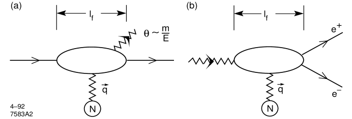
FIG. 6.: Schematic representations of $l_{f}$ for bremsstrahlung and pair conversion, showing their relationship.

Pair production is not possible classically. However, Landau and Pomeranchuk (1953b) give some simple arguments why pair creation should be sensitive to its environment. The momentum transfer for pair production is (Feinberg and Pomeranchuk, 1964)

$$q_{\parallel}=k/c-\sqrt{(k-E)^{2}/c^{2}-m^{2}c^{2}}-\sqrt{E^{2}/c^{2}-m^{2}c^{2}}={m^{2}c^{3}k\over 2E(k-E)}.$$ (57)

Because $q_{\parallel}$ is unchanged when $E$ and $k-E$ are interchanged, either can represent the electron or positron. The formation length can be expressed in terms of the two final state momenta or in terms of the invariant mass of the created pair. Not surprisingly, $l_{f0}$ for pair production is similar to the bremsstrahlung case:

$$l_{f0}={2\hbar E(k-E)\over m^{2}c^{3}k}.$$ (58)

It might seem surprising that $k$ is in the denominator of Eq. (58). But, $l_{f0}$ becomes a maximum for $E=k-E=k/2$; then $l_{f0}=\hbar k/2m^{2}c^{3}$, and $l_{f0}$ rises with $k$. If $E\ll k$, then this equation reduces to $l_{f0}=2\hbar E/m^{2}c^{3}$ and $l_{f0}$ is very short. This asymmetric energy division corresponds to a pair with a large invariant mass. In terms of pair mass, $M_{p}$,

$$l_{f0}={2\hbar k\over M_{p}^{2}c^{3}}.$$ (59)

One difference between pair creation and bremsstrahlung is that the multiple scattering now applies to two separate particles. The lower energy particle scatters more, and so dominates the additional $q_{\parallel}$. The scattering is taken over $l_{f}/2$, as if the charged particles are produced in the middle of the formation zone, and the result is very similar to Eq. (33):

$$l_{f}=l_{f0}\bigg{[}1+{E_{s}^{2}l_{f}\over 2m^{2}c^{4}X_{0}}\bigg{]}^{-1}$$ (60)

where $l_{f0}$ now refers to Eq. (58). When the second term is dominant,

$$l_{f}=l_{f0}\sqrt{kE_{LPM}\over E(k-E)}={2\hbar k\over M_{p}mc^{3}}\sqrt{E_{LPM}\over k},$$ (61)

similar to Eq. (33). Then,

$$S=\sqrt{E_{LPM}k\over E(k-E)}={M_{p}\over m}\sqrt{E_{LPM}\over k}.$$ (62)

For a given $k$, the suppression is largest when $E\approx(k-E)\approx k/2$. There is no suppression for $E\approx 0$ or $E\approx k$. For $E\gg E_{LPM}$, the total cross section scales as $\sqrt{E_{LPM}/k}$. Figures 2 and 10 show how $S$ drops as $k$ rises.

As with bremsstrahlung, the emission angles can affect suppression. The relevant angular variables are $\theta_{e^{+}}$ and $\theta_{e^{-}}$, the angles between the outgoing particles trajectories and the incoming photon path. If either angle is larger than $k/mc^{2}$, then the formation length is shortened and suppression reduced.

Because of the high photon energy, there is no apparent analogy to dielectric suppression for pair creation.

H Muons and Direct Pair Production

Electromagnetic processes involving muons can also be suppressed. However, because the muon mass $m_{\mu}\gg m_{e}$, the effects are much smaller. For a fixed energy, the formation length is reduced by $(m_{e}/m_{\mu})^{2}\sim 1/40,000$. For muons, Eqs. (31) and (35) hold, but with $E_{LPM}$ replaced by

$$E_{LPM(\mu)}={m_{\mu}^{4}c^{7}X_{0}\over\hbar E_{s}^{2}}\approx 1.38\times 10^{22}{\rm eV/cm}\cdot X_{0}.$$ (63)

This energy is high enough that LPM suppression is generally negligible for muon bremsstrahlung and pair creation.

For muons, dielectric suppression still occurs for $y<\hbar\omega_{p}/m_{\mu}c^{2}$, about $10^{-7}$ in solids. This is very small, but perhaps not unmeasurable.

Unlike electrons, high energy muons have a significant cross section for direct pair production, $\mu^{-}N\rightarrow\mu^{-}e^{+}e^{-}N$. This process is similar to bremsstrahlung followed by pair creation, except that the intermediate photon is virtual. Both the $\mu$ and the final state electrons are subject to multiple scattering. The formation length can be calculated by treating the pair as a massive photon, starting from

$$q_{||}=\sqrt{E^{2}-m_{\mu}^{2}c^{4}}-\sqrt{(E-k)^{2}-m_{\mu}^{2}c^{4}}-\sqrt{k^{2}-M_{p}^{2}c^{4}}={m_{\mu}^{2}c^{3}k\over 2E(E-k)}+{M_{p}^{2}c^{3}\over 2k}$$ (64)

where here $E$ is the muon energy, $k$ is the virtual photon energy and $M_{p}$ is the pair mass. Compared to bremsstrahlung, $l_{f}$ is only decreased for $k/E<M_{p}/m_{\mu}$. The final state has three particles that can multiple scatter. Since the incoming muon is very energetic, it exhibits little multiple scattering. The electron and positron are less energetic, and multiple scatter more; the contribution to $q_{||}$ due to (both) their multiple scattering is $E_{s}^{2}M_{p}^{2}l_{f}/4m^{2}kX_{0}$. This is significant (the cross section is reduced) for $l_{f}>(E_{s}/mc^{4})^{2}X_{0}/2$ when $k/E<M_{p}/m_{\mu}$. Suppression is easiest for symmetric pairs because they lead to the longest $l_{f}$, but, even then, energies above $10^{17}$ eV are required to observe suppression.

Although it is much less probable, electrons can also lose energy by direct pair production, $e^{-}N\rightarrow e^{+}e^{-}e^{-}N$. For electrons, $M_{p}>m$, so the second term in Eq. (64) always dominates, and $l_{f}=2\hbar k/M_{p}^{2}c^{3}$. As with muons, suppression occurs for $l_{f}>(E_{s}/mc^{2})^{2}X_{0}/2$, albeit without the restriction on $k/E$. Still, suppression requires energies almost as high as the muon case.

The lack of suppression for direct pair production is an initial demonstration that higher order diagrams typically involve larger $q_{\parallel}$ than simpler reactions. Therefore, higher order processes are less sensitive to their environment, and, when suppression is large, higher order diagrams become more important.

I Magnetic Suppression

External magnetic fields can also affect the electrons trajectory, and hence its radiation. This section will consider the effect of the change in electron trajectory on bremsstrahlung emission, neglecting the closely connected synchrotron radiation emitted by the same field.

An electron will be bent by an angle

$$\theta_{B/2}={\Delta p\over p}={eBl_{f}\sin{\phi_{B}}\over 2E}$$ (65)

in a distance $l_{f}/2$ in a uniform magnetic field $B$. Here, $\phi_{B}$ is the angle between the electron trajectory and the magnetic field. As with multiple scattering, if $\theta_{B/2}>1/\gamma$, then bremsstrahlung is suppressed. This happens when (Klein, 1993)

$$y<y_{B}={\gamma B\sin{\phi_{B}}\over B_{c}}$$ (66)

where $B_{c}$ is the critical magnetic field, $B_{c}=m^{2}c^{3}/e\hbar=4.4\times 10^{13}$ Gauss.

The bending angle $\theta_{B/2}$ accumulates linearly with $l_{f}$, in contrast to the LPM case where $\theta_{MS/2}\sim l_{f}^{2}$; this leads to a stronger $k$ dependence than with LPM scattering. If $\theta_{B/2}$ is treated in the same manner as $\theta_{MS/2}$ in Eq. (29), then

$$l_{f}=l_{f0}\bigg{[}1+\bigg{(}{mcB\sin\phi_{B}l_{f}\over\hbar B_{c}}\bigg{)}^{2}\bigg{]}^{-1}.$$ (67)

This is a quartic equation for $l_{f}$, compared with the quadratic found with multiple scattering. In the limit of strong magnetic suppression ($l_{f}\ll l_{f0}$), the suppression factor $l_{f}/l_{f0}$ has a form similar to the LPM effect (Klein, 1997):

$$S=\bigg{(}{kE_{B}\over E(E-k)}\bigg{)}^{2/3}$$ (68)

where $E_{B}=mc^{2}B_{c}/B\sin{\phi_{B}}$. Figure. 7 shows the suppression for three different values of $E/E_{B}$.

FIG. 7.: Suppression factor $S$ for magnetic suppression, for $E=0.1E_{B}$ (long dashes), $E=1E_{B}$ (solid line) and $E=10E_{B}$ (short dashes).

Because magnetic suppression has a weaker $k$ dependence than dielectric suppression, it is only visible when dielectric suppression does not apply, i.e. for $E>y_{die}E_{B}$, and then for $y_{B}>y>y_{die}$. For 25 GeV electrons in saturated iron ($\sim 20$ kG), $E_{B}\approx 1.5$ PeV and $y_{B}\sim 2.5\times 10^{-5}$, so the magnetic effect will be hidden. At higher electron energies, it becomes quite visible. For a 1 TeV electron in a 4T field, as will be found at in the CMS detector at LHC, photons with energies below 900 MeV are suppressed.

Suppression should also occur for pair production. A similar calculation finds

$$S=\bigg{(}{kE_{B}\over E(k-E)}\bigg{)}^{2/3}.$$ (69)

For symmetric pairs (maximum suppression), $S=(4E_{B}/k)^{2/3}$. Because the magnetic bending is quite deterministic, in contrast to multiple scattering which is statistical, this semi-classical calculation may be more accurate than that for multiple scattering.

Baier, Katkov and Strakhovenko (1988) considered bremsstrahlung suppression in a magnetic field, for both normal matter (screened Coulomb potentials) and $e^{+}e^{-}$ colliding beams. They used kinetic equations to find the radiation to power law accuracy, in both strong and weak field limits. These results are similar to Eq. (68).

When the magnetic field is confined to the material, magnetic suppression should also produce transition radiation. This should be most visible with ferromagnetic materials. Equation (52) could be used to find the spectrum.

Both the semi-classical calculation and the more accurate result neglect synchrotron radiation. Because the formation length scales for bremsstrahlung and synchrotron radiation are similar, they are important in the same kinematic regions. A complete calculation should treat them together, calculating the electron trajectory due to the combined field, and then calculating the radiation for that trajectory.

J Enhancement and Suppression in Crystals

So far, we have considered only amorphous materials. In crystals, however, the regularly spaced atoms produce a huge range of phenomena, because the interactions with the different atoms can add coherently (Williams, 1935). When the addition is in phase, enhanced bremsstrahlung or pair production results, while out of phase addition results in a suppression.

Electrons can interact with atoms with impact parameters smaller than $\hbar/q_{\perp}$. The relative phase depends on the spacing between atoms measured along the direction of electron motion. The phase difference for two interactions is $\Phi=\exp{\{i[\omega t-{\bf k\cdot a}(t)]\}}$ where ${\bf a}$ is the atomic position. If $\Phi$ has the same phase for two nuclei, then the emission amplitudes add coherently.

Including $\theta_{\gamma}$, the phase difference between two adjacent sites is

$$\Phi=\exp{\{i[\omega-{\bf k}\cdot{\bf v}]a\cos(\theta_{\gamma})\}}$$ (70)

where $a$ is the spacing between two atoms along the direction of electron motion. If the nuclei are spaced so that

$$ak\cos(\theta_{\gamma})={4\pi n\hbar E(E-k)\over m^{2}c^{3}}$$ (71)

where $n$ is an arbitrary integer, then $\Phi=1$ and the addition is coherent. As with Čerenkov radiation, for certain $\theta_{\gamma}$, the phase is always zero, and $l_{f}\rightarrow\infty$, implying infinite emission (from an infinite crystal). Conversely, if $ak\cos(\theta_{\gamma})=(2n+1)2\pi\hbar E(E-k)/m^{2}c^{3}$, there is complete destructive interference.

The large set of variables in Eq. (71) gives rise to a variety of effects. As the incident electron direction (affecting $a$) and/or $\theta_{\gamma}$ vary, the interference will alternate between constructive and destructive, producing peaks in the photon energy spectrum for most sets of conditions.

Although Eq. (70) predicts infinite coherence, in a real crystal several factors limit the coherence length. One of these is the thermal motion of the atoms. When the rms thermal displacement of the atoms is larger than $1/q_{\parallel}$, the coherence is lost. When $\theta_{\gamma}$ is large, the transverse separation between the electron and photon can limit the coherence.

Changes in the electron trajectory can also reduce the coherence length. The crystalline structure can generate very high effective fields, causing strong bending, known as channeling (Sørensen, 1996); this bending can limit the coherence length. Multiple scattering can also change the electron direction, and limit the coherence (Bak et al., 1988). Finally, crystal defects and dislocations can also limit coherence. Because this is a vast subject, with several good reviews available (Palazzi, 1968) (Akhiezer and Shul’ga, 1987) (Baier, Katkov and Strakhovenko, 1989) (Sørensen, 1996), this article will not consider regular lattices further.

K Summary & Other suppression mechanisms

The suppression mechanisms discussed so far are summarized in Table II, in order of increasing strength. Many other physical effects can lead to suppression of bremsstrahlung and pair production. Many of them involve partially produced photon interactions with the medium. Some of the interactions that can affect bremsstrahlung are photonuclear interactions, real Compton scattering, and, at lower energies, a host of atomic effects including K and L edge absorption and a variety of optical phenomena.

Photonuclear interactions can have an effect similar to that of pair conversion - the partly created photon is destroyed. Because the photonuclear cross section is much smaller than the pair conversion cross section, this is a small correction. Real Compton scattering can also effectively destroy the photon. Toptygin (1964) treated these reactions as imaginary (absorptive), higher order terms to the dielectric constant of the medium. The bremsstrahlung plus real Compton scattering of the partially produced photon is in some sense a new class of radiation, with its own Feynman diagram. Because Compton scattering involves momentum transfer from the medium, $l_{f}$ is short, and so, in some regions of phase space (when dielectric suppression is large), Toptygin found that this diagram can be the dominant remaining source of emission.

Other photon absorption mechanisms occur at lower photon energies. For example, K or L edge absorption produces a peak in the photon absorption spectrum. If, over a formation length, the absorption probability due to these peaks is significant, then suppression can occur. These peaks are difficult to observe because of competition from transition radiation, which is enhanced at the same energies (Bak et al., 1986). For optical photons, a host of atomic effects can affect the dielectric constant. These variations can also introduce suppression (Pafomov, 1967).

III Migdal formulation

More quantitative calculations are more complex. The first quantum calculation, by Migdal (1956, 1957) is still considered a standard. Migdal treated the multiple scattering as diffusion, calculating the average radiation per collision, and allowing for interference between the radiation from different collisions. When collisions occur too close together, destructive interference reduces the radiation.

This approach replaces the average multiple scattering angle used earlier with a realistic distribution of scattering, and, hence, of of the electron path. Migdal also allows for the inclusion of quantum effects, such as electron spin and photon polarization.

Migdal treated multiple scattering using the Fokker-Planck technique (Scott, 1963). This technique is used to solve the Bolzmann transport equation for $F(\theta,z)$, where $F$ is the probability distribution of particles moving at an angle $\theta$ with respect to the initial direction. The equation is:

$${\partial F(\theta,z)\over\partial z}=-\omega_{o}(z)F(\theta,z)+\int_{0}^{\infty}\theta^{\prime}d\theta^{\prime}\int_{o}^{2\pi}d\beta^{\prime}W(\chi,z)F(\theta^{\prime},z)$$ (72)

where $\omega_{0}$ is the scattering probability per unit thickness, given by the integral of $W(\theta,z)$ over all angles. Here, $\theta$ is the scattering angle and $\beta^{\prime}$ is the azimuthal angle. $W(\chi,z)$ is the single scatter angular distribution. The angle $\chi$ is the angular opening between vector representing $\theta$ and $\theta^{\prime}$: $\chi^{2}=\theta^{2}+\theta^{\prime 2}-2\theta\theta^{\prime}\cos\beta^{\prime}$. The $W$ dependence on $z$ allows for inhomogeneity in the material; otherwise $W$ is independent of $z$. For each of the trajectories allowed by the diffusion, Migdal calculated the photon radiation, including electron spin and photon polarization effects.

The Fokker Planck method is valid if $W(\chi,z)$ is sufficiently sharply peaked at $\chi=0$, so that it has a finite mean square $\langle\chi^{2}\rangle_{z}$ and that $F(\theta^{\prime},z)-F(\theta,z)$ can be accurately approximated by a second order Taylor expansion in $\theta^{\prime}-\theta$. Some calculations (Scott, 1963) lead to a Gaussian distribution for $F$, with a mean multiple scattering angle $\langle\chi^{2}\rangle_{z}$. Unfortunately, a Gaussian distribution underestimates the number of scatters at angles larger than a few times $\theta_{0}$ (Eq. (55)). This problem limits the accuracy of this calculation. The problem is somewhat exacerbated because $l_{f}$ is relatively short, so the number of scatterings is fairly small.

A Bremsstrahlung

With these calculations, updated with a more modern form factor, the Migdal cross section for bremsstrahlung is

$${d\sigma_{\text{LPM}}\over dk}={4\alpha r_{e}^{2}\xi(s)\over 3k}\{y^{2}G(s)+2[1+(1-y)^{2}]\phi(s)\}Z^{2}\ln\bigg{(}{184\over Z^{1/3}}\bigg{)}$$ (73)

where $G(s)$ and $\phi(s)$ are the suppressions of the electron spin flip and no spin flip portions of the cross section respectively,

$$G(s) = 48s^{2}\bigg{(}{\pi\over 4}-{1\over 2}\int_{0}^{\infty}e^{-st}{\sin{(st)}\over\sinh{(t/2)}}dt\bigg{)}$$ (74)

$$\phi(s) = 12s^{2}\bigg{(}\int_{0}^{\infty}e^{-sx}\coth{(x/2)}\sin{(sx)}dx\bigg{)}-6\pi s^{2}.$$ (75)

The factor $\xi(s)$ is

$$\xi(s) = 2\hskip 198.7425pt(s<s_{1})$$ (76)

$$\xi(s) = 1+\ln(s)/\ln(s_{1})\hskip 124.66618pt(s_{1}<s<1)$$ (77)

$$\xi(s) = 1\hskip 198.7425pt(s\geq 1)$$ (78)

with $s_{1}=Z^{2/3}/184^{2}$. Here,

$$s=\sqrt{E_{LPM}k\over 8E(E-k)\xi(s)}.$$ (79)

Migdal gave infinite series solutions for $G(s)$ and $\phi(s)$. However, they may be more simply represented by polynomials (Stanev et al., 1982):

$$\phi(s) = 1-\exp{\bigg{(}-6s[1+(3-\pi)s]+s^{3}/(0.623+0.796s+0.658s^{2})\bigg{)}}$$ (80)

$$\psi(s) = 1-\exp{\bigg{(}-4s-8s^{2}/(1+3.96s+4.97s^{2}-0.05s^{3}+7.5s^{4})}\bigg{)}$$ (81)

$$G(s) = 3\psi(s)-2\phi(s).$$ (82)

These functions are plotted in Fig. 8.

FIG. 8.: Migdals $G(s)$ (dashed line) and $\phi(s)$ (solid line). $\phi$ governs the suppression for $y\ll 1$.

For $k\ll E$, $s\sim 1/\langle\gamma\theta_{MS}\rangle$. For $s\gg 1$, there is no suppression, while for $s\ll 1$, the suppression is large. In the absence of suppression $G(s)=\phi(s)=1$, and Migdal matches the Bethe-Heitler cross section. For small suppression, where $s$ is large, $G(s)=1-0.22/s^{4}$ and $\phi(s)=1-0.012/s^{4}$. For strong suppression, where $s\rightarrow 0$, $G(s)=12\pi s^{2}$ and $\phi(s)=6s$.

If a Coulomb scattering distribution is fit with a Gaussian, the mean of the Gaussian grows slightly faster than $\sqrt{l_{f}}$. This increase is reflected in the the logarithmic rise in $\xi$. For sufficiently high energies, $q_{max}$ is limited by the nuclear radius $R_{A}$, which Migdal approximated $R_{A}=0.5\alpha r_{e}Z^{1/3}$. The nuclear radius limits $q_{max}$ to $\hbar/R_{A}$; at higher momentum transfers the nuclear structure is important and Eq. (73) loses accuracy. The fortuitously simple ‘2’ coefficient comes from the chosen approximation for $R_{A}$. This cutoff is only reached for extremely large suppression, and is hence of limited importance; higher order terms are likely to dominate at this point.

One difficulty with these formulae is that $\xi$ depends on $s$, which itself depends $\xi$, so the equations must be solved recursively. To avoid this problem, Stanev and collaborators (1982) developed simple, non-iterative formulae to find $s$ and $\xi(s)$. They removed $\xi(s)$ from the equation for $s$, defining

$$s^{\prime}=\sqrt{E_{LPM}k\over 8E(E-k)}.$$ (83)

Then, $\xi$ depends only on $s^{\prime}$:

$$\xi(s^{\prime}) = 2\hskip 198.7425pt(s^{\prime}<\sqrt{2}s_{1})$$ (84)

$$\xi(s^{\prime}) = 1+h-{0.08(1-h)[1-(1-h)^{2}]\over\ln{\sqrt{2}s_{1}}}\hskip 33.24467pt(\sqrt{2}s_{1}<s^{\prime}\ll 1)$$ (85)

$$\xi(s^{\prime}) = 1\hskip 198.7425pt(s^{\prime}\geq 1).$$ (86)

where $h=\ln{s^{\prime}}/\ln{(\sqrt{2}s_{1})}$. This transformation is possible because $\xi$ varies so slowly with $s$.

Fig. 9 compares the energy weighted cross section per radiation length, $X_{0}nyd\sigma/dy$, Eq. (73), for several electron energies. As $E$ rises, the cross section drops, with low energy photons suppressed the most. The number of photons with $k<E(E-k)/E_{LPM}$ is reduced.

FIG. 9.: The energy weighted differential cross section for bremsstrahlung, $X_{0}nyd\sigma_{\text{LPM}}/dy$ for various electron energies in a lead target, showing how the spectral shape changes. Electrons of energies 10 GeV (top curve), 100 GeV, 1 TeV, 10 TeV, 100 TeV, 1 PeV and 10 PeV (bottom curve) are shown. The units are fractional energy per radiation length.

Although it reproduces the main terms of the Bethe-Heitler equation, Eq. (73) does not include all of the corrections that are typically used today. Without any suppression, Eq. (73) becomes

$${d\sigma_{\text{LPM0}}\over dk}={4\alpha r_{e}^{2}\over 3k}\{y^{2}+2[1+(1-y)^{2}]\}Z^{2}F_{el},$$ (87)

matching the Bethe and Heitler (1934) result. In comparison a modern bremsstrahlung emission cross section (Tsai, 1974) (Perl, 1994)

$${d\sigma_{\text{BH}}\over dk}={4\alpha r_{e}^{2}\over 3k}\bigg{[}\{y^{2}+2[1+(1-y)^{2}]\}\ \ [Z^{2}(F_{el}-f)+ZF_{inel}]+(1-y){(Z^{2}+Z)\over 3}\bigg{]}$$ (88)

includes several additional terms. $F_{el}$ is the elastic form factor from Sec. 2, $\ln{(184/Z^{1/3})}$, for interactions with the atomic nucleus. $F_{inel}$ is an inelastic form factor, $\ln{(1194/Z^{2/3})}$ that accounts for inelastic interactions with the atomic electrons. Newer suppression calculations, discussed later, treat inelastic scattering separately.

The $f$ term accounts for Coulomb corrections because the interaction takes place with the electron in the Coulomb field of the nucleus. For lead $f=0.33$, while $F_{el}=3.7$. The Coulomb correction may be incorporated into suppression calculations by adjusting the form factors (Sec. VII; Baier and Katkov, 1997a).

These corrections may be accounted for with a simple assumption (Anthony et al., 1995). Since $q_{||}\ll mc$ the target mass is irrelevant for suppression purposes, and the two form factors can be lumped together. The same can be done for the Coulomb corrections. This is done by scaling the radiation length to include these corrections; the standard tables of radiation lengths (Barnett, 1996) include these factors.

The other difference, the final $1-y$ term, is problematic because of the different $y$ dependence. In a semi-classical derivation (Ter-Mikaelian, 1972, pg. 18-20), this term only appears in the no-screening limit, small impact parameter, high momentum transfer, limit, where the formation length is short. So, this term should represent a part of the cross section that involves large momentum transfers, and so is not subject to suppression. Because it is only about a 2.5% correction for large $Z$ nuclei, current experiments have limited sensitivity to this point.

In the strong suppression limit, for $y\ll 1$, the small $s$ approximations for $\phi(s)$ and $\xi(s)$ lead to the semi-classical scaling

$$S=3\sqrt{kE_{LPM}\over E(E-k)}.$$ (89)

Because $\xi(s)$ varies only logarithmically with $s$, this limit, corresponding to $\xi(s)=2$, is only reached for very strong suppressions, $S<10^{-3}$. As Fig. 1 shows, the normalization differs from the semi-classical results, but it, as previously mentioned, can depend on the how the absolute cross section is treated. Moreover, for a direct comparison, it might be fairer to use $\xi=1$, since the semi-classical calculations neglect the relevant non-linear scaling. This changes the coefficient to $3/\sqrt{2}\sim 2$. For lower energies, the strong suppression limit is

$$S\sim\sqrt{{36kE_{LPM}\over 8E(E-k)}\bigg{(}1-0.13\ln{S}\bigg{)}}$$ (90)

where the recursion for $\xi(s)$ has been removed, and $s_{1}$ calculated for lead. It is clear that the correction for $\xi$ is significant, particularly for small $S$.

These calculations contain some sources of error. Because of the Fokker-Planck method and the problematic mean scattering angle; these results are of only logarithmic accuracy. One numerical hint of inaccuracy can be seen by comparing Migdal’s formula with the Bethe-Heitler limit. For $k_{LPM}<k<1.3k_{LPM}$, $\phi(s)\xi(s)$ rises slightly above 1 and the Migdal result is slightly above Bethe Heitler. The maximum excess is about 3%. This can serve as a crude estimate of the expected accuracy of Eq. (73).

Migdal also considered dielectric suppression. Since it only occurs for $y\ll 1$, only the $\phi$ term is relevant; Migdal replaced $\phi(s)$ with $\phi(s\Gamma)/\Gamma$, where $\Gamma=1+k_{p}^{2}/k^{2}$, to get

$${d\sigma_{\text{LPM}}\over dk}={16\alpha r_{e}^{2}\xi(s)\over 3k}{\phi(s\Gamma)\over\Gamma}Z^{2}\ln\bigg{(}{184\over Z^{1/3}}\bigg{)}.$$ (91)

The same substitution applies for the simplified polynomials (Stanev et al., 1982). This is close to the Ter-Mikaelian result, although it misses the modified form factor in Eq. (46).

Equation (73) can also be found with a classical path integral approach (Laskin, Mazmanishvili and Shul’ga, 1984). The radiation for a given trajectory, Eq, (25), can be averaged over all possible paths, In the limit $k\ll E$, required by the classical nature of the calculation, this reproduces Migdal’s result. Dielectric suppression can also be included in the path integral approach (Laskin, Mazmanishvili, Nasonov and Shul’ga, 1985).

Migdal notes that, for thick slabs, the photon angular distribution is dominated by the electron multiple scattering. However, nothing in Migdal’s calculation should change the semi-classical result that suppression should be reduced for photons with $\theta_{\gamma}>1/\gamma$; this effect may be visible in thinner targets. Pafomov (1965) discussed the energy and angular distribution of photons emerging from thin slabs ($T\ll X_{0}$), producing a complex set of results.

B Pair Creation

The cross section for pair production may be found simply by crossing the Feynman diagram for bremsstrahlung, as shown in Fig. 6. Migdal used this crossing to calculate the cross section for pair production:

$${d\sigma_{\text{LPM}}(\gamma\rightarrow e^{+}e^{-})\over dE}={4\alpha r_{e}^{2}\xi(\tilde{s})\over 3k}\bigg{(}G(\tilde{s})+2\big{[}{E^{2}\over k^{2}}+(1-{E\over k})^{2}\big{]}\phi(\tilde{s})\bigg{)}$$ (92)

where

$$\tilde{s}=\sqrt{E_{LPM}k\over 8E(k-E)\xi(\tilde{s})}\approx{mc^{2}\over k\gamma}$$ (93)

and $G$ and $\phi$ are as previously given. In the limit $\tilde{s}\gg 1$ there is no suppression, while $\tilde{s}\rightarrow 0$ indicates large suppression, both leading to the appropriate semi-classical result. These equations can be simplified as was done with bremsstrahlung (Stanev, 1982).

Figure 10 gives the pair production cross section in lead for a number of photon energies. As $k$ increases above $E_{LPM}$, the cross section drops, with asymmetric pairs increasingly favored. For $E_{LPM}<E(k-E)/k<1.3E_{LPM}$, $\phi(\tilde{s})\xi(\tilde{s})>1$ and the Migdal cross section rises above the Bethe-Heitler case, matching the bremsstrahlung overshoot. It also causes the ’hiccup’ present at $k=E_{LPM}$ in Fig. 2.

FIG. 10.: The differential cross section for pair production, $X_{0}nd\sigma_{\text{LPM}}/dy$ in lead for various photon energies, showing how the spectral shape changes. Cross sections are plotted for photons of energies 1 TeV (top curve), 10 TeV, 100 TeV, 1 PeV, 10 PeV, 100 PeV and 1 EeV (bottom curve).

C Surface Effects

Migdal’s calculations only apply for an infinite thickness target. Several authors have calculated the transition radiation due to multiple scattering, based on a Fokker-Planck approach. Although these calculations begin with the same approach, the details differ significantly, as do the final results. Gol’dman (1960) added boundaries to Migdal’s Fokker-Planck equation, calculating the emission inside and outside the target, and an interference term. Outside the target, there is no emission, while inside he reproduced Migdal’s result. For the surface terms, the photon flux for $y\ll 1$ and $s\ll 1$ is

$${dN\over dk}={\alpha\over\pi k}\ln{1\over s}\approx{\alpha\over 2\pi k}\ln{({8k_{LPM}\over k})}$$ (94)

per surface. This result is simlar to the semi-classical result in Eq. (53).

Ternovskii (1960) considered the dielectric effect as well as multiple scattering, again starting from Migdal’s kinetic equation. He considered the entire range of target thicknesses, including interference between closely spaced boundaries. By comparing the radiation inside the target with an interference term, he found that for $T<\alpha X_{0}/2\pi$, multiple scattering is insignificant, and the Bethe-Heitler spectrum is recovered. This is a much broader range than the limit $T<X_{0}/1720$ presented in section II F. His results for intermediate thickness targets, Eq. (54), apply for $\alpha X_{0}/2\pi<T<\alpha X_{0}/2\pi s$, also a wider range than in Sec. II F.

For thicker targets, with $T\gg\alpha X_{0}/2\pi s$, if the dielectric dominates ($s>1$ or $s(k_{p}/k)^{2}>1$), he obtains Eq. (51). Where multiple scattering dominates ($s<1,s(k_{p}/k)^{2}\ll 1$), then

$${dN\over dk}={\alpha\over 2\pi k}\bigg{(}{k^{2}\over E^{2}}+2{E^{2}+(E-k)^{2}\over E^{2}}\bigg{)}\ln{{\chi\over\sqrt{s}}}$$ (95)

where ’$\chi\approx 1$’. This result is similar to Eq. (94), but covers the complete range of $y$. Neglecting the logarithmic term, the spectrum matches that of unsuppressed bremsstrahlung for a target of thickness $\sim 0.5\alpha X_{0}$. This has a different $E$ and $k$ dependence than would result from $1\ l_{f}$ of Bethe-Heitler radiation.

Unfortunately, Eq. (95) is difficult to use. It only applies for $s(k_{p}/k)^{2}\ll 1$; no solution is given for the intermediate region $s(k_{p}/k)^{2}\sim 1$. Also, $\chi$ is poorly defined. If the equation is extended to $s(k_{p}/k)^{2}=1$, then choosing $\chi=1$ creates a large discontinuity. The discontinuity disappears for $\chi=0.42$, but this also eliminates transition radiation in the region $0.17<s<1$.

Garibyan (1960) extended his previous work with transition radiation to include multiple scattering. He found that multiple scattering dominates for $k>k_{cr}$, matching the semi-classical result for infinite targets. If $\xi(s)$ is neglected, this is the same cutoff found by Ternovskii. Where multiple scattering dominated, he reproduced Eq. (94). Elsewhere, he found the usual transition radiation from the dielectric of the medium.

Equations (94) and (95) are negative for $s>1$; common sense indicates that they should be cut off in this region where no transition radiation is expected. However, Pafomov (1964) considered this evidence that these works were wrong. He stated that they incorrectly separated the radiation into transition radiation and bremsstrahlung. He calculated the transition radiation as the difference between the emission in a solid with and without a gap, again starting with the Gol’dman’s initial formulae. Pafomov found that multiple scattering dominated transition radiation for $k>k_{cr}$. Surprisingly, he found that multiple scattering affected transition radiation even for $E<y_{die}E_{LPM}$, with an additional term $dN/dk=\alpha/\pi k(k_{LPM}/k)^{2}$ added to the conventional result when $k>k_{p}$. For $k_{LPM}>k_{p}$, he found different formula for different $k$. For $k<k_{cr}$

$${dN\over dk}={\alpha\over\pi k}=\ln{k_{cr}^{2}\over k^{2}}$$ (96)

while for $k_{cr}<k<k_{LPM}$,

$${dN\over dk}={\alpha\over\pi k}\ln{{2\over 3}\sqrt{k_{LPM}\over k}}.$$ (97)

Counterintuitively, Pafomov predicted that for $k>k_{LPM}$, there is still transition radiation, with

$${dN\over dk}={\alpha\over\pi k}\ \ {8k_{LPM}^{2}\over 21k^{2}}.$$ (98)

These two equations do not match for $k=k_{LPM}$. However, a numerical formula, not repeated here, covers the entire range smoothly. It is worth noting that Eq. (98) is quite close to the semi classical result for $k<k_{LPM}$.

Fig. 11 compares the transition radiation from a single surface predicted by Gol’dman/Garibyan, Ternovskii (using $\chi=1.0$), and Pafomov. Except for Pafomov, these calculations predict radiation up to $k=k_{LPM}=E^{2}/E_{LPM}$. For a flat $kdN/dk$ spectrum, the total energy radiated per surface rises as $E^{2}$, as with the semi-classical approach. For large enough $E$, electrons lose most of their energy to radiation when crossing an interface.

FIG. 11.: Comparison of the edge effects predicted by Ternovskii (with $\chi=1$) (solid line) and Pafomov (long dashes), for a single independent edge, compared with conventional transition radiation (short dashes). (a) shows the radiation from a 100 GeV electron in lead. The jump in the Ternovskii curve at $k=350$ keV is at $s(k_{p}/k)^{2})=1$, while the drop in the Pafomov curve at 630 keV is at $k=k_{cr}$. Panel (b) shows the Pafomov and Ternovskii predictions for a 10 TeV electron in lead; both curves are much smoother. Conventional transition radiation is negligible in (b).

However, these equations fail before this point. For high enough electron energies, these calculations predict that each electron should emit several photons per edge traversed. Since the formation lengths for the various photon emissions will overlap at the edge, this is really a higher order process, not yet treated properly by calculations.

Unfortunately, these calculations appear to do a poor job of fitting the data. Fig. 19 shows that they predict transition radiation considerably above the data from SLAC E-146.

IV Blankenbecler and Drell formulation

Blankenbecler and Drell (1996) calculated the magnitude of LPM suppression with an eikonal formalism used to study scattering from an extended target. The approach was originally developed to study beamstrahlung. One major advantage of their approach is that it naturally accommodates finite thickness slabs, automatically including surface terms.

They begin with a wave packet that scatters while moving through a random medium. For each electron path, they calculate the radiation, based on the acceleration of the electron. The radiation is calculated for all possible paths and averaged. One clear conceptual advantage of this calculation is that it does not single out a single hard scatter as causing the bremsstrahlung; instead all of the scatters are created equal. This differs from Landau and Pomeranchuk and Migdal, who found the rate of hard scatters which produced bremsstrahlung, and then calculated the multiple scattering in the region around the hard scatter to determine the suppression. For a thick target, in the strong suppression limit $s\ll 1$, they predict that the radiation is $\sqrt{3\pi/8}$ (about 8%) larger that of Migdal.

One advantage of this calculation is that it treats finite thickness media properly. There are three relevant length scales: $l_{f0}$ (Eq. (5)), $T$ and $\alpha X_{0}$. Blankenbecler and Drell (1996) called $\alpha X_{0}$ the mean free path for elastic scattering, based on counting vertices in Feynman diagrams. This correspondence does not stand up to more detailed examination. However, the arguments in the paper are not affected. These variables are combined into two ratios:

$$N_{BD}={\pi l_{f0}\over 3\alpha X_{0}}$$ (99)

and

$$T_{BD}={\pi T\over 3\alpha X_{0}}$$ (100)

where $T_{BD}$ is the target thickness, in mean free paths, while $N_{BD}$ is the number of formation lengths per mean free path; when $N_{BD}$ is large suppression is strong, while $N_{BD}<1$ corresponds to a single interaction per electron, i.e. the Bethe Heitler regime.

The eikonal approach finds the wave function phase and momentum difference between different points on the electron path. These differences are then used to find the radiation for that length scale. The probability of emission from the target is

$${dP_{BD}\over dk}={\alpha\over 2kE(E-k)\hbar^{2}c^{2}}\int{d^{2}k_{\perp}\over 4\pi^{2}}\int_{-\infty}^{+\infty}dz_{2}\int_{-\infty}^{z_{2}}dz_{1}S(z_{2},z_{1})\cos\bigg{(}\int_{z_{1}}^{z_{2}}dz{d\Phi(z,0)\over dz}\bigg{)}.$$ (101)

Here, $k_{\perp}=k\cos(\theta_{\gamma})$ is the photon perpendicular energy, $S(z_{2},z_{1})$ is a sum over electron polarization (spin flip and no spin flip) of the squared perpendicular momentum acquired by the electron due to scattering, and $d\Phi/dz$ is the differential phase difference due to the scattering. The $d^{2}k_{\perp}$ integration is equivalent to an integration over photon angles. In the absence of scattering, $d\Phi/dz$ is constant, and then the integrals must be carefully evaluated; Blankenbecler and Drell introduce a convergence factor to insure that the boundary conditions are correct.

Because the integrals include all possible values of $z$, three regions must be considered: before the target (denoted $+$), inside the target (denoted $0$), and after the target ($-$). For the double integral, there are 9 possible combinations, of which two ($++$ and $--$) are clearly zero. Time ordering eliminates ($-+$), ($-0$) and ($0+$), leaving the bulk term ($00$), two single surface terms ($+0$) and ($0-$) and an interference term ($+-$). For thick targets with $T_{BD}\gg 1$, the interference term vanishes, and the bulk term dominates over the single surface terms. In this case, their calculations reproduce the Migdal results, with the 8% higher cross section. For thinner targets, the surface terms are more important. Figure 12 compares these terms, using a suppression form factor $S=F(N_{BD},T_{BD})$ relative to Bethe-Heitler.

FIG. 12.: The Blankenbecler and Drell form factor $F(N_{BD},T_{BD})$ for a target with $T_{BD}=10$, showing the contributions for the bulk emission ($00$) and the transition and interference terms $(0-)$, ($+0$) and ($+-$). For a fixed target thickness, $N_{BD}\sim 1/l_{f0}\sim k/E^{2}$; the edge effects are largest for small $N_{BD}$ corresponding to small $k$. From Blankenbecler and Drell (1996).

For thin targets, $T_{BD}<1$, where $N_{BD}>1$, the interference term ($+-$) dominates, demonstrating a large transition radiation. $N_{BD}/T_{BD}<1$ reduces to the Bethe Heitler free particle case.

For a thick target, $T_{BD}>1$, the central interaction ($00$) region is important. For large $N_{BD}$, their results are similar to those of Migdal. For very large $N_{BD}$, with $N_{BD}>T_{BD}$, the formation length is longer than the target, and both the ($00$) and mixed regions contribute. Fig. 13 compares the suppression as a function of $N_{BD}$ (which is proportional to $1/k$), for a variety of $T$. For large $T_{BD}$, suppression increases with $N_{BD}$. When $T_{BD}$ decreases, suppression drops, eventually becoming almost independent of $N_{BD}$, at a value similar to that predicted by Shul’ga and Fomin (1996).

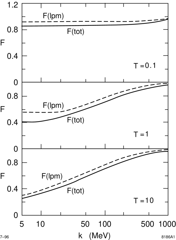
FIG. 13.: The Blankenbecler and Drell form factor $F(N_{BD},T_{BD})$ for 25 GeV electrons in 3 thicknesses of gold targets. F(lpm), assumes that the wave function amplitude and phase fluctuate independently, while F(tot) includes the correlation between amplitude and phase, further reducing the emission. From Blankenbecler (1997b).

There are a few caveats in this calculation. The eikonal approach assumes that the potential is smooth enough. Blankenbecler and Drell used a Gaussian scattering potential, which underestimates the rate of large angle scattering. Second, they assumed that the wave function phase and amplitude fluctuate independently. Blankenbecler (1997b) showed that the correlation between amplitude and phase reduces the emission by a further 5-15%. Figure 13 compares curves with and without the correlation. The calculation has also been extended to include multiple slabs separated by a gap (Blankenbecler, 1997a).

Calculating the emission from a slab as a whole is problematic, These results assume that there is either zero or one interaction per incident electron. But, for a typical bremsstrahlung cross section of 10 photons per $X_{0}$, the relative probability of getting 2 interactions compared with 1 interaction is $\sim 20T/X_{0}$, so single interactions are only prevalent for slabs with $T<0.05X_{0}$. This problem makes it difficult to apply these results in many real-world situations.

V Zakharov calculation

Zakharov (1996a,b, 1998a,b) transformed the problem of multiple scattering into a two dimensional (impact parameter and depth in the target) Schröedingers equation. The imaginary potential is proportional to the cross section for an $e^{+}e^{-}$ pair scattering off of the atom, which is itself simply related to the bremsstrahlung cross section. This equation was solved using a transverse Greens function based on a path integral. This impact parameter approach is complementary to Migdal’s momentum space approach. Because this approach allows for arbitrary density profiles, it naturally accommodates finite thickness targets.

Zakharov (1996a) calculated the radiation due to a simple Coulomb potential. The calculation is keyed to the scattering cross section for a $e^{+}e^{-}$ dipole of separation $\rho$, $\sigma(\rho)=C(\rho)\rho^{2}$. In the strong suppression limit, $C$ varies slowly with $\rho$. Zakharov then found the frequency $\Omega$ for a harmonic oscillator in a potential which would reproduce this scattering cross section. This is roughly equivalent to describing the multiple scattering with a Gaussian. The radiation is governed by a parameter $\eta=\Omega l_{f}$. For an infinitely thick target, the results are almost identical to Migdal (Zakharov, 1998a); functions of $\eta$ that match Migdal’s $\phi(s)$ and $G(s)$, for $\eta=1/\sqrt{8}s$. The only difference is the slowly varying part of the cross section: $\xi(s)$ for Migdal and $C(y\rho_{\rm eff})/C(\hbar c/m)$ for Zakharov; $\rho_{\rm eff}$ is the impact parameter where radiation is largest. In the Bethe-Heitler limit, $\rho_{\rm eff}\sim\hbar c/ym$.

In the limit $y\rightarrow 0$, for strong suppression

$${d\sigma_{Z}\over dk}={2\alpha^{2}Z\over E}\sqrt{2\hbar c\log{(2a/y\rho_{\rm eff})}\over\pi nk}$$ (102)

where

$$\rho_{\rm eff}=\bigg{(}{\pi Z^{2}\alpha^{2}nEy^{3}\log{(2/\alpha Z^{1/3})}\over\hbar c}\bigg{)}^{1/4}$$ (103)

where $a$ is the Thomas-Fermi screening radius Numerically, $\rho_{\rm eff}({\rm m})\sim 10^{-9}/[E{\rm(eV)}y^{3}]^{1/4}$ for lead. These equations are valid for $200/Z^{1/3}<\log(2a/y\rho_{\rm eff})<1.5\times 10^{5}/Z^{2/3}$; corresponding to Migdal’s $\xi(s)=1$ and $\xi(s)=2$.

Except for the ‘1’ in $\xi(s)$, this equation has the same form as Migdal’s Eq. (90). Although unimportant to the theory, the ‘1’ greatly reduces the effect of the slowly varying term. Numerically, $2a/y\rho_{\rm eff}=6.8\times 10^{-7}E(eV)/y$ for lead; other solids aren’t too different. For a 1 TeV electron beam, as $y$ varies from $10^{-4}$ (a typical $y_{die}$) to $10^{-2}$ (an arbitrary upper limit to ’low $y$’), the Zakharov logarithm varies by about 20%, while the change in $\xi(s)$ is much smaller. This variation should be measureable.

For moderate suppression, a more detailed treatment is required. Because $C(\rho)$ varies more quickly with $\rho$, the harmonic oscillator approximation fails and the actual potential must be used (Zakharov, 1996b). Zakharov used separate screened elastic ($a=0.83a_{0}Z^{-1/3}$) and inelastic ($a=5.2a_{0}Z^{-2/3}$) potentials, reproducing the appropriate unsuppressed bremsstrahlung cross sections. The separate potentials are most important for low $Z$ nuclei. However, because of the small recoil, the separate form factors have a small effect on suppression. The more complicated potential requires additional integrations. Because of this, this approach can so far be used only for finite thickness targets.

Figure 14 shows Zakharov’s suppression factors for finite target thicknesses in a 25 GeV electron beam. This demonstrates how suppression increases with target thickness. The thickest target, with $h=10$ is very close to the infinite thickness limit. Zakharov (1998b) added a correction to allow for multiple photon emission, and did a detailed comparison with SLAC E-146 data. Except for the carbon targets in 25 GeV electron beams, he found good agreement with the data for photon energies $k>5$ MeV (above the region of dielectric suppression).

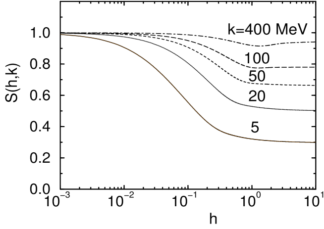
FIG. 14.: Suppression factor $S(h,k)$ found by Zakharov. The curves are for a 25 GeV electron, with $h=T/l_{f0}$. The $h=10$ results are very close to the infinite thickness limit. The dip around $h=1$ for the highest photon energies is due to interference between the two target surfaces. From Zakharov (1996b).

Zakharov (1997b) presents a few results for multiple-slab configurations, finding a smaller interference term than Blankenbecler (1997a). The two results would agree better if Blankenbecler included the amplitude-phase correlation in his multiple slab calculations.

Zakharov’s results for gluon bremsstrahlung from a quark will be discussed in Sec. XII.

VI BDMS Calculation

The BDMS group (R. Baier et al., 1996) started with the Coulomb field of a large number of scatterers, with the atomic screening modelled with a Coulomb potential cut off with a Debye screening mass $\mu$. An eikonal approach is used to account for the large number of scatters.

The critical variable in this calculation is the (dimensionless) phase difference between neighboring centers,

$$\kappa={X_{0}\mu^{2}c^{3}k\over 2\hbar E^{2}}$$ (104)

For QED calculations, $\mu=\hbar Z^{1/3}/a_{0}c$ reproduces Thomas-Fermi screening. The authors also define a coherence number $\nu=\alpha l_{f0}/X_{0}$, the number of scatters required for the accumulated phase shift to equal 1. This $\nu$ is similar to Blankenbecler and Drells $N_{BD}$. A large phase shift between interactions, $\kappa>1$, corresponds to the Bethe-Heitler limit. Because this approach assumes massless electrons, its ’Bethe-Heitler limit’ does not completely match the usual Bethe-Heitler formula.

In the factorization limit, $T<l_{f0}$, where the entire target reacts coherently, their results match Ternovskii (1960):

$${dN\over dk}={2\alpha\over\pi k}\langle\ln({q_{tot}^{2}\over m^{2}c^{2}})\rangle$$ (105)

where $q_{tot}$ is the total perpendicular momentum acquired by the particle while traversing the target due to multiple scattering. Here, the mass $m$ is introduced to remove a collinear divergence.

In the LPM regime, ($\kappa\ll 1)$, the bremsstrahlung cross section is similar to Eq. (102). The logarithmic term is due to non-Gaussian large angle ($\theta>1/\gamma$) Coulomb scatters. Because of these large scatters, the mean squared momentum transfer is poorly defined, and, in fact, diverges logarithmically; this logarithm appears in the suppression formula.

$${d\sigma\over dk}\sim{\alpha\over\pi kX_{0}}\sqrt{\kappa\ln{(1/\kappa)}}.$$ (106)

They comment that they neglect a logarithmic factor under the logarithm; if the corresponding term is removed from Zakharov’s formula, the two results have the same functional dependence. If one identifies $E_{LPM}=\kappa\mu^{2}/2$, as their paper indicates, then the radiation takes the form

$${d\sigma\over dk}\sim{\alpha\over\pi k}\sqrt{{kE_{LPM}\over E^{2}}\log{E^{2}\over kE_{LPM}}}.$$ (107)

VII Baier & Katkov

Baier and Katkov (1997a) also studied suppression due to multiple scattering, trying to reach an accuracy of a few percent, by including several corrections omitted previously. They begin with the scattering from a screened Coulomb potential, in the same impact parameter space used by Zakharov. Coulomb corrections are included to account for the motion of the screening electrons, along with separate potentials for elastic and inelastic scattering. Finally, they allow for a nuclear form factor, with an appropriately modified potential for impact parameters smaller than the nuclear radius.

They find the electron propagator for a screened Coulomb potential, in the Born approximation. This assumes Gaussian distributed scattering, and reproduces Migdal’s result. The electron propagator is then expanded perturbatively, with a correction term which accounts for both large angle scatters and Coulomb corrections to the potential. Without the Coulomb corrections, the first order result is similar to that of Zakharov (V. Baier, 1998).

Coulomb corrections are incorporated by adjusting the parameters in the potential. With Coulomb corrections, the screening radius becomes $a_{2}=0.81Z^{-1/3}a_{0}\exp[0.5-f(Z\alpha)]$. while the characteristic scattering angle changes from $\theta_{1}=\hbar c/Ea_{0}$ to $\theta_{2}=\hbar c/Ea_{0}\exp[f(Z\alpha)-0.5)]$. Here, $f(Z\alpha)$ is the standard Coulomb correction (Tsai, 1974). This scaling accounts for the extra terms in Eq. (88) compared with Eq. (87). For heavy nuclei, $a_{2}$ is about 20% larger than the Thomas-Fermi screening radius.

Higher order terms may also be calculated for the electron propagator. The ratio of the first two terms of the expansion is $0.451$ divided by a logarithmic term, so the series should converge reasonably rapidly.

Inelastic scattering can be included by adding a term to the scattering potential, changing the charge coupling from $Z^{2}$ to $Z^{2}+Z$ and further modifying the characteristic angle, to $\theta_{e}=\theta_{1}\exp{[Z/(1+Z)(f(\alpha Z)-1.88)-0.5]}$.

Dielectric suppression is included by modifying the potential, with a replacement similar to Migdal’s. For $k\ll k_{p}$, the spectrum is similar to Ter-Mikaelian’s, but with power law and Coulomb corrections:

$${d\sigma\over dk}={16Z^{2}\alpha r_{e}^{2}k\over 3k_{p}^{2}}\bigg{[}\ln{\bigg{(}{184k_{p}\over kZ^{1/3}}\bigg{)}}+{1\over 12}-f(Z\alpha)\bigg{]}$$ (108)

where $f(Z\alpha)$ is the standard Coulomb correction (Tsai, 1974).

Baier and Katkov considered the extremely strong suppression regime, neglected by Migdal, where the finite nuclear radius becomes important. This region is reached at the lowest $E$ for $y\ll 1$, where dielectric suppression otherwise dominates. There, limiting $q$ (i.e. $q_{\parallel}$) to $\hbar/R_{A}$ changes the form factor for $k<k_{p}R_{A}\lambda_{e}$. In lead, this corresponds to $y<2\times 10^{-6}$. Then,

$${d\sigma\over dk}={16Z^{2}\alpha r_{e}^{2}k\over 3k_{p}^{2}}\bigg{(}\ln{({a\over R_{A}})}-0.02\bigg{)}.$$ (109)

For $y=10^{-6}$ in lead, this is about 25% larger than Eq. (108). This is probably measurable, although transition radiation and backgrounds will be very large.

Baier and Katkov then considered targets with finite thicknesses, breaking down the possibilities in a manner similar to Blankenbecler and Drell, with a similar double integral. For relatively thick targets, $T>l_{f0}$, the results are consistent with Ternovskii (1960), but with additional terms for the Coulomb correction. For $T<l_{f0}$ and strong suppression,

$${dN\over dk}={\alpha\over\pi k}\bigg{[}{k^{2}\over E^{2}}+\bigg{(}1+{(E-k)^{2}\over E^{2}}\bigg{)}\bigg{(}(1+{1\over 2A})[\ln{(4A)}-0.578]+{1\over 2A}-1+{0.578\over L_{t}}\bigg{)}\bigg{]}$$ (110)

where $A=\pi Z^{2}\alpha^{2}nT\hbar^{2}/m^{2}c^{2}(L_{t}+1-2\times 0.578)$ and $L_{t}\sim 2\ln{(2a_{2}/\lambda_{e}\rho_{t})}$, with $\rho_{t}$ the (scaled) minimum impact parameter that contributes to the form factor integral. Unfortunately, this equation diverges as $T\rightarrow 0$.

V. Baier and Katkov (1997a) compared their photon spectrum with SLAC E-146 data from a $0.02X_{0}$ thick tungsten target in 25 and 8 GeV electron beams, and find good agreement. However, a target this thick has a substantial (roughly 20%) correction to the photon spectrum to account for electrons that undergo two independent bremsstrahlung emissions. This correction is not included in their calculation, and the good agreement with data is surprising. A later work (Baier and Katkov, 1999) included multiphoton effects, and also finds good agreement with the data; the difference between the two calculations is not explained.

V. Baier and Katkov (1997b) considered thinner targets with $T\sim l_{f0}$. They compare their calculations with SLAC E-146 data, for 0.7 % $X_{0}$ thick gold targets in 8 and 25 GeV beams, and also find good agreement. Because this target is much thinner, the multiple interaction probability is greatly reduced and the agreement is not surprising.

VIII Theoretical Conclusions

A Comparison of Different Calculations

The calculations discussed here used a variety of approaches to solve a very difficult problem. Because the underlying techniques are so different, it is difficult to compare the calculations themselves. However, some general remarks are in order.

All of the post-Migdal calculations are done for a finite thickness slab, integrating both bulk emission and transition radiation. Unfortunately, the finite thickness slab calculations are not easily usable by experimenters, because they assume each electron undergoes at most one interaction in the target. Multiple interactions are easily accounted for in a Monte Carlo simulation. However, the simulation must be able to localize the photon emission, while these calculations are for the slab as a whole. Because of the edge terms, it isn’t correct to simply spread the emission evenly through the slab. This limits their direct applicability to thin slabs.

The newest calculations by Zakharov and Baier and Katkov include multiple photon emission. However, these calculations are still for bulk targets, and are not very amenable to complex geometries. For example, these calculations could not be used to model an electromagnetic shower.

Here, we will use the Migdal approach as a standard for comparison. Although Zakharov’s approach is very different from Migdal, he reproduces Migdal’s result in the appropriate limit. However, Zakharov incorporates some further refinements which should lead to increased accuracy. Baier and Katkov have a similar approach to Zakharov, and include a number of additional refinements, especially for bremsstrahlung at very low $y$.

The other works have very different genealogies. Because the BDMS result does not reproduce the Bethe-Heitler limit, it is more relevant to QCD than QED. However, if the formalism is extended to include hard radiation, and some additional graphs are added, then BDMS becomes equivalent to the Zakharov formalism (R. Baier et al., 1998b).

For Blankenbecler and Drell, the only obvious point of comparison is the potential; Zakharov (1996b) states that the Blankenbecler and Drell potential does not match the Coulomb potential, and will not show the logarithmic dependence given by the slow variation of $C(\rho)$ or $\xi(s)$.

The results can also be compared numerically. Unfortunately, these calculations are very complex and the descriptions frequently lack adequate information for independent computation. So, it is necessary to rely on the results given by the authors. One point of comparison is defined by SLAC E-146 data on a thin target: 25 GeV electrons passing through a 0.7 % $X_{0}$ thick gold target. The E-146 data agreed well with Migdal as long as $T>l_{f}$; at lower $k$, Ternovskii’s Eq. (54) matched the data. Blankenbecler and Drell, Zakharov, and Baier and Katkov all showed good agreement with this data. Zakharov initially added in a 7% normalization factor to match the data. Some correction is required, because, even for a 0.7% $X_{0}$ target, the multiphoton pileup ‘correction’ is still several percent. With a correction for multiphoton emission Zakharov (1998b) found normalization coefficients average 1, except for the uranium targets. Zakharov also changed his approach to Coulomb corrections between the two works. The other authors do not discuss normalization. Overall, in this energy range, the different approaches agree with each other to within about 5%.

Because of the different logarithmic treatment, Migdal, Blankenbecler and Drell, and Zakharov will scale slightly differently with energy. Changes depending on target thickness are more complicated; the surprising agreement found by Baier and Katkov for the 2% $X_{0}$ tungsten data, where multiple interactions are a 20% correction, shows that there there are significant uncertainties in scaling the results with target thickness. It would also be interesting to compare the calculations for a low $Z$ target, where the E-146 data showed some disagreement with Migdal.

B Very Large Suppression

One weakness of all of these calculations is that they only consider the lowest order diagrams. For fixed $y$, $l_{f}$ rises with $E$, even with LPM suppression. At high enough energies, the formation zones from different emissions will overlap, and any lowest order calculation will fail. Dielectric suppression is strong enough that $l_{f}$ decreases and localization improves with increasing suppression, so it is less subject to this problem. However, for multiple scattering, a method of dealing with higher order terms is needed. While the radiative corrections to bremsstrahlung are known (Fomin, 1958), they were not computed with suppression mechanisms in mind.

Even neglecting the overlapping formation zones, when suppression is large, higher order terms are important, because higher order processes involve larger $q_{\parallel}$, and hence are less subject to suppression; Sec. II.H illustrated this for direct pair production. So, when suppression is strong ($S\sim\alpha$), current calculations are suspect. For QCD calculations, discussed in Sec. XII the problem is much worse because of the large coupling constant, $\alpha_{s}$.

It is worth noting that suppression can affect other processes, via radiative corrections. The total cross section for Coulomb scattering, for example, is the sum of the elastic cross section plus the cross section for bremsstrahlung where the photon is not observable. Since suppression can affect the latter process, it can indirectly change the elastic scattering cross section (Ter-Mikaelian, 1972, pg. 135). Inelastic processes, which leave the target atom in an excited state can also contribute significantly to the cross section when suppression of the lowest order diagrams is large.

C Classical and Quantum Mechanical Approaches

There has been some controversy as to how well classical electrodynamics can predict LPM suppression. The original Landau and Pomeranchuk (1953a,b) calculations were completely classical; they failed at the same point that classical bremsstrahlung calculation fail: when $k\sim E$. The path integral approach (Laskin, Mazmanishvili and Shul’ga, 1984) goes further, and reproduces Migdal’s result in the same limit. Of course, at least semi-classical calculations are necessary for pair production.

The main advantage of quantum mechanical calculations is that it covers the complete range of $y$. The newest calculations include features not found in the classical approaches. However, some of the advances, such as separate elastic and inelastic potentials could certainly be included in a classical calculation.

In the future, quantum approaches appear necessary to calculate the higher order terms that become important at extremely high energies, when formation lengths from different emissions begin overlapping. Unfortunately, these calculations seem extremely difficult, and are probably a long way off.

However, the classical approach to LPM suppression was not universally accepted. Bell (1958) stated that Migdal’s predictions conflicted with classical electrodynamics, and concluded that “any real effect of this kind is of essentially quantal origin.” He pointed out that the classical radiation, Eq. (6), is positive definite, and hence monotonically increasing for increasing pathlength. However, Bell neglected to account for the fact that, in a dense solid, the electron trajectory ${\bf r}(t)$ changes, and one cannot simply sum the radiation due to interactions with separate nuclei. Even classically, emission from the different pieces of electron pathlength can interfere, in a manner similar to other classical interference effects.

IX Experimental Results

Bremsstrahlung or pair creation suppression can be studied with high energy electron or photon beams. Because pair creation suppression requires photons with $k>E_{LPM}$, beyond the reach of current accelerators, pair creation has been studied only with cosmic rays, with consequently very limited statistics. The best suppression studies have used electron beams at accelerators. Besides the LPM effect, these beams have been used to study dielectric suppression.

A Cosmic Ray Experiments

The first tests of LPM suppression came shortly after Migdal’s paper appeared. These experiments used high energy ($k>1$ TeV) photons in cosmic rays, and studied the depth of pair conversion in a dense target. The earliest experiments looked for a deficiency of low energy electrons in electromagnetic cascades (Miesowicz, Stanisz and Wolther, 1957). This analysis is difficult because of uncertainties in the incoming photon spectrum and electron energy measurement.

Fowler, Perkins and Pinkau (1959) studied isolated pair production in an emulsion stack. They measured the shower energy and the distance between the initial conversion and the first daughter pair resulting from the primary. They observed 47 showers with $k>1$ TeV. As $k$ increased, the distance between the conversions rose, as predicted by Migdal, contrasting with with decrease predicted by Bethe- Heitler.

Varfolomeev and collaborators (1960) used a similar approach, albeit on a smaller data set, with similar results. They selected events where the energy of the daughter pair was very small ($y\ll 1$), and found qualitative evidence for suppression; they did not differentiate between LPM and dielectric suppression.

Lohrmann (1961), studied emulsion exposed on high altitude balloon flights. Compared to earlier results, Lohrmann studied lower energies, where the LPM and Bethe-Heitler cross sections are much closer. However, the increased photon flux allowed for much better statistics, making up for the smaller cross section difference. Lohrmann used a variety of analysis techniques, all of which supported Migdal’s results. More recently, long duration balloon experiments have gathered somewhat larger data samples, up to 120 events, with similar results (Strausz et al., 1991).

Kasahara (1985) studied the development of $\sim$100 TeV showers in lead/emulsion chambers exposed to cosmic rays on Mt. Fuji. His analysis was based on the fact that electromagnetic LPM showers with $E\gg E_{LPM}$ penetrate considerably more material than Bethe-Heitler showers. Kasahara found that the shower development profiles matched simulations based on Migdal, but differed from his Bethe-Heitler simulations. The study suffered from a background from hadronic and/or multiple photon showers, both also subject to large fluctuations. Kasahara removed 5 obvious background events from his initial 19 event sample, but warned that some of the remainder could also be hadronic. This study is of special interest as it is the only study yet in the region $E\gg E_{LPM}$, where suppression affects shower development.

All of the air shower experiments suffered from some common problems, by far the largest being the poor statistics; high enough energy photons are not common. In addition, because of the limited emulsion thickness, they did not consider surface effects. Finally, uncertainties in the photon spectrum complicated the analysis. For these reasons, these experiments are at best qualitative verifications of LPM suppression.

B Early Accelerator Experiments

By the 1970’s, 40 GeV electron beams were available at Serpukhov, and the first accelerator based test of LPM suppression was done there (Varfolomeev et al., 1975). Bremsstrahlung photons from 40 GeV electron beams striking dense targets were detected in an sodium iodide calorimeter. The electrons were magnetically bent away from the calorimeter. Photons with 20 MeV $<k<$ 70 MeV emitted from carbon, aluminum, lead and tungsten targets were studied. Below 20 MeV, synchrotron radiation from the bending magnets dominated the measurement, while above 70 MeV, the experiment was insensitive to the spectral change predicted by Migdal.

The experiment suffered from several limitations. Because the electron beamline was in air, and included several scintillation counters used as triggers, there was a significant light element bremsstrahlung background. The experimenters also mention a significant background due to muon contamination in their beam.

The collaboration presented their data in terms of ratios of photon spectra: lead/aluminum and tungsten/carbon. This may have been done to account for events containing several bremsstrahlung photons from a single electron. The data showed suppression in the region that Migdal predicted. However, the degree of suppression was larger than Migdal predicted, although within the large errors.

CERN NA-43 was an experiment dedicated to studying channeling radiation from electrons and positrons in crystals (Bak et al., 1988). In channeling, electrons or positrons travel along the crystal rows, and hence are strongly affected by the coherently adding fields from the atom rows. At large angles to the axes, the coherence disappears, and normal bremsstrahlung occurs. In this large angle regime, they saw suppression which they attributed to LPM suppression. They also observed suppression consistent with multiple scattering for electrons incident along one of the crystal rows. This is slightly different from suppression in an amorphous material; here the suppression is really the loss of coherent enhancement.

The first experimental studies of dielectric suppression were part of a larger study of transition radiation (Arutyunyan, Nazaryan and Frangyan, 1971). Although the experiment focused on studies of emission from stacks of thin radiators, the experimenters also measured the radiation from 0.25 and 2.8 GeV electrons traversing relatively thick glass and aluminum targets. Although few details were given, they appeared to observe suppression in the expected energy range.

C SLAC E-146

In 1992, the E-146 collaboration at Stanford Linear Accelerator Center (SLAC) proposed an experiment to perform a precision measurement of LPM suppression, and to study dielectric suppression (Cavalli-Sforza et al., 1992). The experiment was conceptually similar to the Serpukhov experiment, but heavily optimized to minimize background. To minimize the statistical errors, the experimenters collected a very large data set. The experiment was approved in December, 1992, and took data in March-April, 1993.

1 Experimental Setup

Figure LABEL:e146layout shows a diagram of the experiment. An 8 or 25 GeV electron beam entered SLAC End Station A and passed through a thin target. The targets used are listed in Table III. The beam was then bent downward by a 3.25 T-m dipole magnet, through six wire chamber planes which measured electron momenta and into an array of lead glass blocks which accurately counted electrons. Produced photons continued downstream 50 meters into a BGO calorimeter array. To minimize backgrounds, the electron path visible to the calorimeter and the photon flight path were kept in vacuum.

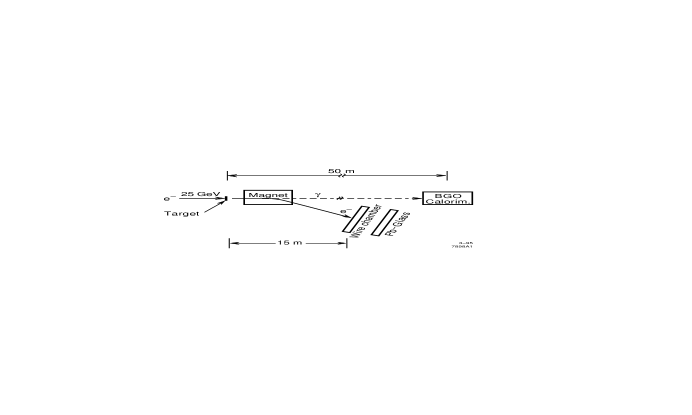
FIG. 15.: Diagram of the SLAC-E-146 apparatus. From Anthony et al. (1995).

The calorimeter comprised 45 BGO crystals in a 7 by 7 array with missing corners; each crystal was 2 cm square by 20 cm (18 X₀) deep. This segmentation provided excellent spatial resolution for separating synchrotron radiation from bremsstrahlung photons. Scintillation light from each crystal was measured separately by a photomultipler tube (PMT). The light yield was about 1 detected photoelectron per 30 keV, providing good statistics down to 200 keV. The calorimeter resolution was about 8% (FWHM) at 100 MeV, with a nonlinearity of about 3%. The calorimeter temperature was monitored throughout the experiment, and the data corrected using the measured drifts.

The collaboration used several methods to calibrate the calorimeter, to obtain both an absolute energy calibration and a crystal to crystal intercalibration. The primary tools for measuring the relative gain were nearly vertical cosmic-ray muons, selected by a plastic scintillator paddle trigger; the gain in each crystal channel was adjusted to produce equal signals.

The absolute energy scale of the calorimeter was primarily determined using a 500 MeV electron beam. This calibration was checked with data by comparing the electron energy loss, measured by the wire chamber, with the calorimeter energy measurement. Because of the steeply falling photon spectrum and the non-Gaussian errors in the momentum measurement, this was useful only as a cross-check.

Because of the large bremsstrahlung cross section, the experiment required a beam intensity of about 1 electron per pulse. Because it would have been very uneconomical to use the SLAC linac to produce a single electron per pulse, the collaboration developed a method to run parasitically during SLAC linear collider (SLC) operations, by using the off-axis electrons and positrons that are removed from the beam by scrapers in the beam switchyard (Cavalli-Sforza et al., 1994).

Normally, about 10% of the SLC beam is scraped away by collimators in the last 200 meters of the linac. The collimators are only 2.2 X₀ thick, so a usable flux of high energy photons emerged from their back and sides. Some of these photons travel down the beampipe, past the magnets that bend the electrons and positrons into the SLC arcs, and into the beam switchyard, where a 0.7 $X_{0}$ target converted them into $e^{+}e^{-}$ pairs. Some of the produced electrons were captured by the transport line optics, collimated, selected for energy, and transported into the end station.

The beam worked well, with the size, divergence and yield matching simulations. At 8 and 25 GeV, the beam intensity was adjustable up to about 100 electrons/pulse. At 1 electron/pulse, the beam emittance was limited by the optics, with a typical momentum bite of $\Delta p/p<0.5\%$.The beam optics were adjusted to minimize the photon spot size at the calorimeter; spot sizes there were typically a few mm in diameter. The beam spot was stable enough and small enough that beam motion was not a major source of error.

Data was collected and written to tape on every beam pulse (120 Hz). With the beam intensity averaging 1 electron/pulse, over 500,000 single electron events could be collected per eight hour shift. The experiment ran for a month, and good statistics were obtained with a variety of targets.

2 Data Analysis and Results

The E-146 analysis selected events containing a single electron, as counted by the lead glass blocks. The photon energy was found by summing the energies of hit BGO crystals using a cluster-finding algorithm. The cluster finding reduced the noise level by eliminating random noise hits.

The experiment studied the photon energy range from 200 keV to 500 MeV, a 2500:1 dynamic range. This exceeded the linear dynamic range of the PMTs and electronics, so data was taken with two different PMT gains, varied by changing the PMT high voltage. The high-$k$ running corresponded to 1 ADC count per 100 keV and the low-$k$ running was 1 ADC count per 13 keV, with the relative gains calibrated with the cosmic ray data. The high-$k$ data was used for 5 MeV $<k<$ 500 MeV while the low-$k$ data covered 200 keV $<k<$ 20 MeV, with a weighted average used in the overlap region.

These two sets of data differed in several significant ways. There were large differences in calorimeter behavior and background levels, as well as the physics topics. For $k>10$ MeV, photons largely interacted by pair conversion, producing an electromagnetic shower. Showers typically deposited energy in 3-20 crystals in the calorimeter. For $k<2$ MeV, the photons interacted by single or multiple Compton scattering. Usually, Compton scattering deposited energy in a single calorimeter crystal. Sometimes, the photon Compton scattered once and then escaped from the calorimeter, taking some energy with it. This added a low energy tail to the energy deposition curve. While the high-$k$ data had very low backgrounds, the low-$k$ data had significant backgrounds due to synchrotron radiation, at least for the 25 GeV beams. Finally, the two data sets emphasize different physics, with the high-$k$ data most relevant for LPM suppression, with the low-$k$ data more useful for studying dielectric suppression. For these reasons, the two sets of data were analyzed quite independently, and combined in the final histograms.

3 Backgrounds and Monte Carlo

One advance introduced by E-146 was the use of a detailed, high statistics Monte Carlo. The main purpose of the Monte Carlo was to understand multi-photon pileup. This occurred when a single electron passing through the target interacted twice, radiating two photons. The Monte Carlo also simulated photon absorption in the target (Anthony et al., 1997) and modelled the detector. Transition radiation was treated as an integral part of the physics, rather than a background. In addition to conventional transition radiation, the predictions of Ternovskii and Pafomov were included as options.

The Monte Carlo tracked electrons through the material in small steps, allowing for the possibility of bremsstrahlung in the material and transition radiation at each edge. LPM suppression was implemented using simple formulae (Stanev et al., 1982) with dielectric suppression incorporated using Eq. (91). For consistency, the Bethe-Heitler cross sections were included by turning LPM suppression off from Migdal’s formulae, rather than using a more modern formula.

The expected and measured backgrounds were both small. The major background was synchrotron radiation from the spectrometer magnet. Synchrotron radiation was significant for $k<1$ MeV in the 25 GeV data. Because the magnet bent the beam downward, the synchrotron radiation painted a stripe in the calorimeter, extending downward from the center. Because of the large lever arm, and because the bending started in the fringe field of the magnet, where the field was low, the synchrotron radiation was small near the center of the calorimeter. Because of the good spatial resolution of the calorimeter, most of the synchrotron radiation was removed with a cut on the photon position in the calorimeter; photons within $45^{o}$ of a line downward from the calorimeter midpoint were removed; this cut removed most of the synchrotron radiation, along with 25% of the signal.

Non-target related backgrounds were measured with target empty runs. The backgrounds were typically 0.001 photons with $k>200$ keV per electron, much less than the $\sim 10T/X_{0}$ bremsstrahlung photons with $k>200$ keV per electron. Target related backgrounds were expected to be small; photonuclear interaction rates are small, and the events are unlikely to appear in the E-146 analysis.

4 Results

Because of the high statistics and low background, the E-146 data allowed for detailed tests of the theory; photon spectra could be easily compared with different predictions.

Figures 16-20 show a sampling of E-146 results. Photon energies were histogrammed logarithmically, using 25 bins per decade of energy, so that each bin had a fractional width $\Delta k\sim 10\%k$. The logarithmic scale is needed to cover the 2500:1 energy range. The logarithmic binning $dN/d\ln k=kdN/dk$ was chosen so that a $1/k$ Bethe-Heitler (BH) spectrum will have an equal number of events in each bin, simplifying the presentation and statistical analysis.

Figure 16 shows the photon spectrum (points with error bars) from 8 and 25 GeV electrons passing through 2% and 6% $X_{0}$ carbon targets. Also shown are 3 Monte Carlo (MC) histograms. The top histogram (dashed line) is a simulation of BH bremsstrahlung plus conventional transition radiation; the transition radiation is substantial below $k_{p}$, 1.4 (0.4) MeV at 25 (8) GeV. Above $k_{p}$, the spectrum is sloped because there is a finite probability of a single electron interacting twice while passing through the target. Because the calorimeter cannot separate single photons from multiple hits, but instead measures total energy deposition, this depletes the low energy end of the spectrum (shown here), while increasing the number of calorimeter overflows. In the absence of multiple interactions, the Bethe-Heitler spectrum would be flat at $(1/X_{0})dN/d\ln k=4/3\ln{(k_{max}/k_{min})}=0.129$ for bins with logarithmic widths $k_{max}/k_{min}=10^{1/25}=1.096$. The bin heights directly scale with the bin fractional width $\Delta k/k$.

FIG. 16.: Comparison of data from SLAC-E-146 with MC predictions for 200 keV to 500 MeV photons from 8 and 25 GeV electrons passing through 2% and 6% $X_{0}$ carbon targets. The cross sections are given as $dN/d(\ln k)/X_{0}$ where $N$ is the number of events per photon energy bin per incident electron, for (a) 2% $X_{0}$ carbon and (b) 6% $X_{0}$ carbon targets in 25 GeV electron beams, while (c) shows the 2% $X_{0}$ carbon and (d) the 6% $X_{0}$ carbon target in an 8 GeV beam. Three Monte Carlo curves are shown. The solid line includes LPM and dielectric suppression of bremsstrahlung, plus conventional transition radiation. Also shown are the Bethe-Heitler plus transition radiation MC (dashed line) and LPM suppression only plus transition radiation (dotted line). Adapted from Anthony et al. (1997).

The dotted histogram is a simulation that includes LPM suppression, but not dielectric suppression, plus conventional transition radiation. The solid line includes LPM and dielectric suppression, along with conventional transition radiation. This was the ’standard’ E-146 choice for simulation.

Both suppression mechanisms are required to approach the data. However, there are still significant discrepancies between the LPM plus dielectric MC and the data. Below 800 keV (350 keV) for 25 (8) GeV beams, the upturn in the data may be residual background, especially synchrotron radiation. The difference at higher photon energies is more complex, and will be discussed in the following subsection.

Figure 17 shows the spectrum from 8 and 25 GeV electrons passing through 3% and 6% $X_{0}$ aluminum targets. The same three simulations are shown. Because aluminum has twice the $Z$ of carbon, LPM suppression is considerably enhanced, with $k_{LPM}$ 8 MeV and 800 keV at 25 and 8 GeV respectively. Because the density is similar to carbon, dielectric suppression is similar. Because dielectric suppression dominates for $k<k_{cr}$, the curve for both suppressions is similar to that of carbon. The agreement between the data and the standard curve is better than with carbon.

FIG. 17.: Comparison of data from SLAC-E-146 with Monte Carlo predictions for 200 keV to 500 MeV photons from 8 and 25 GeV electrons passing through 3% and 6% $X_{0}$ aluminum targets. The format and Monte Carlo curves are the same as in Fig. 16. Adapted from Anthony et al. (1997).

Figure 18 shows the spectrum from 8 and 25 GeV electrons passing through 3% and 6% $X_{0}$ iron targets, with just the ’standard’ MC. The general slope of the data matches the simulation, but the behavior at higher $k$ for 25 GeV beams is quite different.

FIG. 18.: SLAC-E-146 measurements and Monte Carlo predictions for 8 and 25 GeV electrons passing through a 3% and 6% $X_{0}$ iron targets. The Monte Carlo curve is based on LPM and dielectric suppression, plus conventional transition radiation. Adapted from Anthony et al. (1997); Panel (c) is mislabelled as 6% $X_{0}$ there.

Figure 19 shows the bremsstrahlung spectra in uranium targets. Uranium is dense enough that LPM suppression is dominant, and the E-146 collaboration compared simulations with dielectric and LPM suppression, plus conventional transition radiation (TR), or the calculations of Ternovskii (1960) or Pafomov (1964) of transition radiation due to multiple scattering.

FIG. 19.: SLAC E-146 measurements and Monte Carlo for 3% $X_{0}$ and 5% $X_{0}$ uranium targets in 8 and 25 GeV electron beams. The solid line shows the LPM and dielectric suppression, conventional transition radiation Monte Carlo prediction. The other lines include simulations based on calculations of transition radiation due to Pafomov (dashed line) and Ternovskii (dotted line), Eq. (95), with $\chi=1$. The flat solid line in panel (a) is a calculation based on Eq. (54). Adapted from Anthony et al. (1997).

The Pafomov curve jumps at $k=k_{cr}$, around 800 keV (400 keV) at 25 (8) GeV, corresponding from the switch from Eq. (96) to a numerical approximation for Eqs. (97) and (98). For $k<k_{cr}$, Pafomov is considerably above the data and the conventional TR curve. Above the jump, the curve shows a reasonable trend, but the TR appears to be several times too high.

The Ternovskii curve also jumps, at $sk_{p}^{2}/k^{2}=1$, about 500 keV (below 200 keV) for the 25 (8) GeV data. Below the jump, Ternovskii matches conventional TR. Above it, Ternovskii is quite far above the data. Moreover, it extends to too high an energy, above $k_{LPM}$. The Ternovskii radiation could be reduced by lowering $\chi$ below 1 in Eq. (95). However, a considerable adjustment would be required.

Figure 20 shows the spectrum from 8 and 25 GeV electrons passing through a 0.7% $X_{0}$ gold target. The solid histogram is the standard simulation. This target is especially interesting because, at 25 GeV, for $k<7$ MeV, $T<l_{f0}$. Including LPM suppression, $T<l_{f}$ for $k<3$ MeV, and the target should interact as a single unit. The BH $1/k$ spectrum should be recovered, albeit at a reduced intensity. The dot-dashed line shows a calculation based on Eq. (54), in good agreement with the flattening observed in the data. For the E-146 2% $X_{0}$ lead (not shown here) and 3% $X_{0}$ uranium 25 GeV data, Eq. (54) also applies, but only for a very limited range of $k$. However, as Fig. 19 shows, for 3% $X_{0}$ uranium, Eq. (54) predicts $dN/d(\ln k)=0.038$ for 1.0 MeV $<k<$ 3.7 MeV, considerably above the data. The lead data shows a similar discrepancy. Of course, these discrepancies may be because the equation is does not apply so close to $T=l_{f}$.

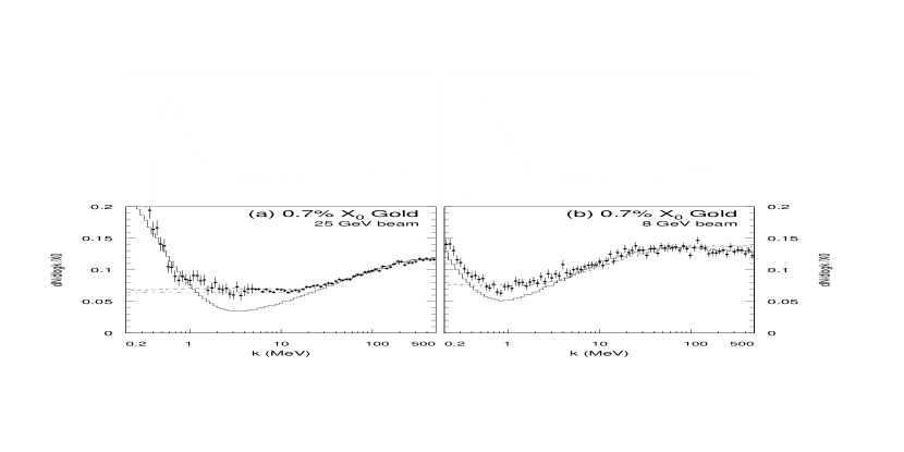
FIG. 20.: SLAC E-146 data on 8 and 25 GeV electrons hitting a 0.7% $X_{0}$ gold target. Shown are calculations by Blankenbecler and Drell (dashed line), and Shul’ga and Fomin (dot-dashed line). For comparison, the Migdal MC is shown as the usual solid line. Adapted from Anthony et al. (1997).

Fig. 20 also shows the results of a calculation by Blankenbecler and Drell. Neither prediction has been corrected for multiple interactions in the target or detector resolution. Because neither calculation includes dielectric suppression or transition radiation, they fail for $k<k_{cr}$.

Fig. 21 shows the spectrum from 8 and 25 GeV electrons hitting a 0.07% $X_{0}$ target. This target is only about $1.2\times(X_{0}/1720)$ thick, so that multiple scattering should produce little suppression, and the Bethe-Heitler simulation (dashed histogram) should be a good match to the data. Dielectric suppression should also be small, because the total phase shift in the target, $\hbar^{2}\omega_{p}^{2}T/k^{2}l_{f}$, is small for $k>500$ keV. Transition radiation should also be strongly suppressed, by $(T/l_{f})^{2}$. Without this suppression, transition radiation would completely dominate the data. As expected, the 25 GeV electron data matches the Bethe-Heitler spectrum. However, the 8 GeV data drops off for $k<2$ MeV. For comparison, a dielectric suppression only Monte Carlo simulation is shown. The data is considerably above this curve.

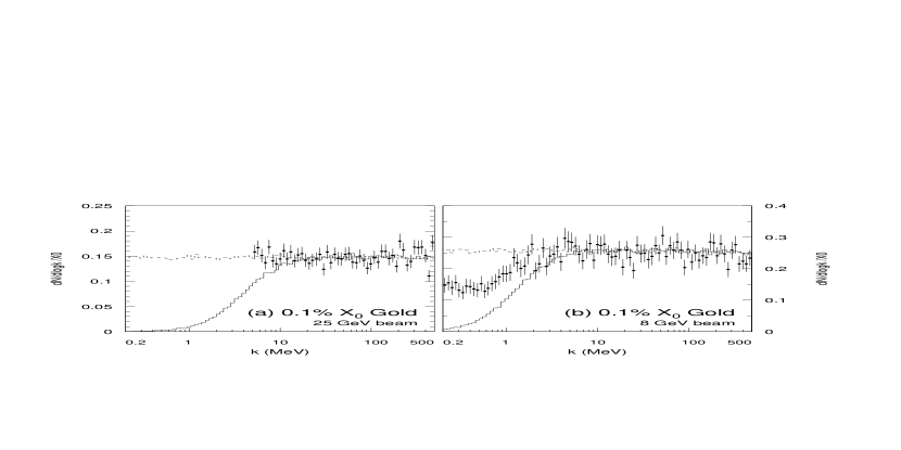
FIG. 21.: Measurements and Monte Carlo for a 0.1% $X_{0}$ gold target at (a) 25 GeV and (b) 8 GeV. The dashed line is the BH prediction (no suppression), while the solid line is a Monte Carlo which includes dielectric suppression, but not LPM suppression. Because the very thin target should exhibit little transition radiation, no transition radiation is included in these Monte Carlos. From Anthony et al. (1997).

Blankenbecler and Drell (Blankenbecler, 1997c) predict that, at 25 GeV, emission is suppressed by 10% compared to BH for k= 500 MeV, rising to 13% at k=100 MeV. At 8 GeV, the difference is only a few percent. Unfortunately, these predictions differ from Bethe-Heitler by less than the experimental errors.

For a target this thin, the collaboration has noted that the signal is very small and the potential backgrounds are large. Furthermore, the target thickness and overall normalization between the signal and simulations cannot be well determined.

In all of these these plots, the Monte Carlo curves were normalized to the data by multiplication by a constant adjustment, chosen so the MC best matches the data above 20 MeV (2 MeV) at 25 (8) GeV. The thresholds were chosen to avoid thin target corrections for $T<l_{f0}$, backgrounds and transition radiation; for the 0.7% $X_{0}$ target, higher limits were chosen, 30 (10) MeV at 25 (8) GeV. Overall, the standard Monte Carlo curves had to be scaled up by an average of 5% (2$\sigma$) to match the data. This discrepancy would likely disappear with an input cross section where the onset of suppression was more gradual around $k\sim k_{LPM}$.

The errors shown on the plots are statistical only. The E-146 collaboration has carefully studied the systematic errors on these measurements. The point-to-point systematic errors vary slowly with $k$ and correspond to a 4.6% uncertainty for $k>5$ MeV. Below 5 MeV, the systematic errors rise to 9%, because of increased uncertainties in photon energy cluster finding as Compton scattering takes over from showering as the dominant energy loss. The $\pm 3.5\%$ systematic error on the normalization was determined separately.

D Bulk versus Surface Effects and Conclusions

Although the data clearly demonstrates LPM and dielectric suppression, the thinnest targets show excess radiation over the bulk LPM predictions. This can easily be ascribed to surface radiation. As long as interference between the two target edges is negligible, the surface and bulk effects can be separated in a model independent way by subtracting spectra from targets made of the same material, but different thicknesses.

Figure 22 shows the results of this subtraction for uranium. Because the subtraction exacerbates the effects of multiple interactions in the target, it is necessary to compare the subtracted spectra with similarly treated simulations. For all of the E-146 materials, the subtracted spectra and simulations agree more closely than the unsubtracted spectra, and, for most targets, the agreement is within the statistical and systematic errors. The notable exceptions are the 25 GeV iron and carbon data.

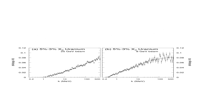
FIG. 22.: Bin by bin subtraction of the 3% $X_{0}$ uranium data from the 5% $X_{0}$ data by SLAC E-146, for 25 and 8 GeV beams. The solid line is the result when the same procedure was applied to their standard Monte Carlo. From Anthony et al. (1997).

The improved agreement indicates that the discrepancies in the unsubtracted spectra are due to surface effects. For the denser targets, this fits the expectations for transition radiation. However, for the lighter carbon and iron targets, the unsubtracted data indicates more suppression than expected. This implies that there is negative emission from the surfaces, an extremely unlikely result.

The collaboration (Anthony et al., 1997) considered a few explanations for the discrepancies. For carbon, the increased suppression could be due to the crystalline structure of the pyrolitic graphite target. If the target density profile varied, then the higher density regions would show more suppression, and the aggregate would show somewhat higher LPM and dielectric suppression. For iron, magnetization of individual domains could produce some magnetic suppression. Unfortunately, the details depend on the (unknown) domain structure.

The density profile could also vary if the target surfaces were oxidized. For the $2\%X_{0}$ tungsten target, the collaboration saw some evidence for this; thickness measurements based on weighing (giving results in $g/cm^{2}$) were lower than those obtained with calipers; an oxide layer could explain this. The anomalous normalization on the 2% tungsten target could also be explained by an oxide layer. For the lighter targets, a surface layer could explain the shapes of the curves, but the required thickness seems very unrealistic, and, in any case, the presence of such a layer is not supported by the normalization and thickness measurements.

It is also possible that Migdal’s theory may be inadequate for lighter targets. However, Zakharov (1998b) also found a very poor fit for the E-146 carbon data, despite a careful treatment of inelastic electron-electron interactions. In comparison, his fits to the other data were quite good. It is possible, although probably unlikely, that a different treatment, would find a better fit. It is also possible that a calculation taking into account the chemical structure of the pyrolitic graphite and using screening based on the actual electron density might better fit the data.

The subtraction procedure could be modified to measure the transition radiation spectrum from a single surface. However, the errors are slightly too large for the result to be interesting.

Overall, the E-146 heavy target data is in good agreement with most of the recent treatments of LPM suppression. However, the shape of the spectra from the lightest targets remain a bit of a mystery.

X LPM effect in Plasmas

So far, we have considered particles moving through a medium. However, in a plasma, there is no separate incident particle, and each particle must be treated on an even footing. If the medium is sufficiently dense, there can be suppression even for non-relativistic particles. Then, the formation time $t_{f}$ is easier to use than the formation length. If $t_{f}$ is longer than the mean time between collisions $t_{c}=1/\Gamma$, $\Gamma$ being the collision rate, then emission can be suppressed.

One hadronic example of a plasma is a supernova; with the high temperature and density, $t_{c}$ is very short. For reactions with $t_{f}>t_{c}$, suppression may be present. One interesting reaction is the production of right handed neutrinos or axions through $NN\rightarrow NN\nu\overline{\nu}$, $nn\rightarrow npe\overline{\nu}_{e}$ and $NN\rightarrow NNa$. If these hypothetical particles exist and are produced, they will carry energy away from the explosion, increasing the cooling rate. The measured cooling rate has been used to put limits on these particles (Raffelt and Seckel, 1991).

For axions or neutrinos, $t_{f}=\hbar/\Sigma E$, where $\Sigma E$ is the sum of the neutrino energies or the axion energy. When $t_{c}\ll t_{f}$, then ’free’ collisions are rare. Instead, the interacting nucleons are excited, This can be modelled by giving the nucleon an effective mass, as may be done with photons in dielectric suppression. Two complications come from the possibility of back reactions, and from the degeneracy of the incoming particles. The suppression is the ratio of the emission $Q(\Gamma)$ to $Q(\Gamma=0)$:

$$S={t_{f}\over t_{f0}}=\bigg{\langle}{\Sigma E^{n+2}\over\Sigma E^{2}+\Gamma^{2}/4}\bigg{\rangle}\langle{1\over\Sigma E^{n}}\rangle.$$ (111)

Here, $n$ accounts for the multiplicity of the emitted particles, with $n=2$ for axions and $n=4$ for neutrino pairs; for axions this equation matches Eq. (43). Because $\Gamma$ depends on the local density; finding the overall suppression factor for an entire supernova requires detailed modelling. However, Raffelt and Seckel estimate that $S$ could be as small as 0.1. So, far fewer axions and neutrinos are emitted than if suppression were absent, and earlier limits that neglect this reduction are invalid (Raffelt and Seckel, 1991).

The general solution for an non-equilibrium electromagnetic plasma has been elegantly formulated using non-equilibrium quantum field theory (Knoll and Voskresensky, 1995, 1996). By careful classification of diagrams, and appropriate resumnation, Knoll and Voskresensky avoided infrared divergences, and reproduced both the classical (non-suppressed) and quasi-particle (low density) limits by appropriate choice of subsets of graphs. In a dense plasma, the quasi-free scattering approximation breaks down, and the reaction rate is reduced by

$$S={k^{2}\over k^{2}+\Gamma^{2}}.$$ (112)

This equation also matches Eq. (43), with $\gamma\hbar\omega_{p}$ of the medium replaced by $\Gamma$, the relaxation rate of the source.

A plasma like this might surround a quantum black hole. Before a quantum black hole explodes, it emits a huge flux of charged particles. This radiation forms a nearly thermal photosphere, consisting of electrons, positrons and photons (Heckler, 1995). The charged particle emission rate and consequent density is high enough that bremsstrahlung and pair production should be suppressed in this plasma. Since most of the emitted particles are hadrons, the black hole may also generate a dense color plasma, akin to a quark gluon plasma, with interactions suppressed as discussed in the following section.

Similar plasma effects probably occurred during the big bang. Unfortunately, we do not know of any calculations involving it.

XI Electromagnetic Showers

Although the LPM effect is best studied using single interactions in thin targets, most real world situations involve electromagnetic showers in thick targets. This includes natural processes like cosmic ray air showers and neutrino induced electromagnetic showers, and showers in man-made detectors. Although modelling showers with suppression effects requires complex analytic calculations or Monte Carlo simulations, this section will present some simple calculations that show when suppression effects can be important.

Suppression affects showers in several ways. Besides the obvious elongation when $E>E_{LPM}$ and the radiation length increases, the shower changes form, with the low energy ’fuzz’ disappearing, and shower to shower fluctuations become much more important, because the number of interactions drops greatly.

A Natural Showers

Many calculations have concerned high energy shower development in water or ice, an area relevant to high energy neutrino astronomy, or in air, an application motivated by extremely high energy (EHE) cosmic ray air showers. The latter case is complicated because the air density varies exponentially with altitude.

Water and ice showers are of interest for detecting very high energy astrophysical $\nu_{e}$ through resonant $W$ production, $\nu_{e}e\rightarrow W\rightarrow e\nu_{e}$ and similar reactions. This cross section rises rapidly at the W pole, corresponding to a $\nu_{e}$ initial energy of 6.4 PeV, an average of 2.1 PeV of which goes to the outgoing electron. Since 2.1 PeV$\sim 7E_{LPM}$, LPM suppression is significant. As Fig. 2 shows, the electron radiation length is increased by about 35%. Since $E\sim 4E_{p}$, pair creation will also cause suppression for a range of $k$.

At similar energies, the search for $\nu_{\tau}N\rightarrow\tau N\rightarrow e\nu_{\tau}\overline{\nu}_{e}N$ events (Learned and Pakvasa, 1995) in ice requires distinguishing the $\tau$ track from the beginning of an electron shower; when suppression mechanisms reduce the number of low energy bremsstrahlung photons, this separation becomes more difficult.

Because both applications involve very high energy showers, direct simulations have been limited by the available computer power; until recently at least partially analytic calculations were needed. These analytic methods owe much of their history to earlier analytic calculations of Bethe-Heitler shower development.

One of the first analytic calculations (Pomanskii, 1970) showed that the penetrating power of electromagnetic showers rises as the LPM effect becomes important. At $10^{19}$-$10^{20}$ eV in earth, electrons and photons become as penetrating as muons. Misaki (1990) used the matrix method to show that EM showers above $10^{15}$ eV in water are elongated by the LPM effect. In the tails of the shower, at a given sampling depth, the LPM effect roughly triples the density.

Unfortunately, while analytic calculations can determine the average shower shape, they have limited value for understanding shower to shower variations; for this, simulations are needed. To reduce the computing load, hybrid Monte Carlos are often used. A hybrid MC simulates the initial shower development; shower tails are added on based on a library of simulated complete showers. This reduces the computational requirements significantly. Stanev and collaborators (1982) measured shower elongation in water and lead due to the LPM effect using a hybrid MC.

Konishi et al. (1991) used a hybrid MC to study fluctuations in a regime where suppression is very strong: $10^{17}$ eV showers in lead. In contrast to BH showers, LPM showers showed large shower to shower variations. By eliminating soft bremsstrahlung, the LPM effect greatly reduces the number of interactions per radiation length, so the shower development depends on far fewer interactions, greatly increasing the shower to shower variation. The variation complicates energy measurement, especially for detectors with limited sampling. Misaki (1993), quantified the degree of fluctuation, measuring the distribution of the depth of shower maximum, the depth at which the number of shower particles is a maximum. For $10^{17}$ eV showers in rock ($E_{LPM}=77$ TeV), he found that shower maximum occurs at $18\pm 13$ (FWHM) $X_{0}$ for BH showers, compared with $152\pm 176$ $X_{0}$ for LPM showers. Not only is the maximum deeper, but its position varies much more.

Not considered here is the increased angular spreading caused by suppression. Although it may be not affect the general shower shape, it is probably important in understanding radio waves produced by showers in ice (Zas, 1997), where the spectrum depends on the transverse separation between particles.

B Cosmic Ray Air Showers

Cosmic ray air showers occur when EHE cosmic rays hit the earths atmosphere and interacts to produce a cascade of particles (Sokolsky, Sommers and Dawson, 1992). Showers up to $3\times 10^{20}$ eV have been seen (Bird et al., 1994). Two techniques are used to study the highest energy air showers. Large aperture telescopes, like the Flys Eye (Bird et al., 1994) observe the shower induced fluorescence of the $N_{2}$ in air, measuring the shower development in the atmosphere. Ground based arrays of hundreds or thousands of small detectors, spaced up to a kilometer apart, observe the remnants of the shower that reach the ground (Takeda, 1998) (Auger, 1996).

Ground based detectors act as calorimeters with a single sampling layer, located behind a 28 $X_{0}$, or 15 hadronic interaction lengths, $\lambda$ thick atmospheric absorber. For a vertical $10^{20}$ eV shower, sea level is near shower maximum, so measurements are not too sensitive to the position of the first interaction. For obliquely incident showers, the detector is considerably behind shower maximum, and as a result, ground observations are subject to significant fluctuations depending on the position of the first interaction. Because of their limited ground coverage, most of their samples are many Moliere radii from the shower core, in the tails of the angular distribution. This heightens the sensitivity of the detector to the details of the initial interactions.

On the other hand, air fluorescence detectors measure the whole shower profile, with the atmosphere acting as a fully active sampling medium. They are thus less sensitive to the details of the shower development.

There has been considerable disagreement about whether the LPM effect is important in ultra-high energy showers. Capdevielle and Attallah (1992) found that LPM suppression had a significant effect on $10^{19}$ to $10^{20}$ eV proton induced air showers. However, Kalmykov, Ostapchenko and Pavlov (1995) found a much smaller change; for a $10^{20}$ eV shower, they found a 5% decrease in the number of electrons at shower maximum, and a $15\pm 2$ g/cm² downward shift in the position of shower maximum. Although this shift is smaller than the measurement resolution, it is systematic, and important in studies of cosmic ray composition. Kasahara (1996) found that the LPM effect reduces the number of particles reaching the ground by about 10% for a $5\times 10^{20}$ eV proton shower. None of these authors considered the effect of other suppression mechanisms.

Although a complete Monte Carlo simulation is required to quantify the effect of suppression, simple calculations can illustrate some qualitative features of shower development (Klein, 1997). The calculations depend strongly on the identity of the incoming particles, with protons (or neutrons) the most popular, although photons or heavier nuclei cannot be excluded. For heavy ions, suppression is greatly reduced because of the lower per-nucleon energy. Because this model is very simple, the possibility of photons pair converting in the earth’s magnetic field will be neglected (Kasahara, 1996)(Stanev and Vankov, 1997). The probability depends on the photon energy and the angle between the photon and the earths magnetic field. For primary photons with $k>10^{20}$ eV, the probability is large, partly because the magnetic field extends to much higher altitudes than the atmosphere.

Because the atmospheric pressure, $1/X_{0}$ and $1/E_{LPM}$ decrease exponentially with height, it is convenient to use an exponential depth variable such as column density. Column density is measured in g/cm², with ground level, $A_{0}$ at 1030 g/cm². Then, $E_{LPM}=(A_{0}/A)$ 234 PeV, where $A$ is the depth in column density. Similarly, $y_{die}=1.3\times 10^{-6}(A/A_{0})$ and $E_{p}=\sqrt{A_{0}/A}\ 42$ PeV. Because the atmosphere is much cooler at high altitudes, these numbers underestimate suppression by about 25%. They also neglect the fact that air is composed of diatomic $N_{2}$ and $O_{2}$ molecules; when an electromagnetic interaction involves one atom of the molecule, the other atom will introduce additional multiple scattering over that expected from a monoatomic gas. This could be a significant effect, but it has yet to be studied.

Incoming photons react by pair production, while protons interact hadronically. A central hadronic collision will produce a shower of several hundred pions; the neutral pions will decay to photons. The highest energy $\pi^{0}$ will have a rapidity near to the incoming proton, and their decay photons will have energies up to $2\times 10^{19}$ eV. Many diffractive processes, such as $\Delta$ production can also produce photons with similar energies. Overall, photons from central interactions will have an average energy of about $2\times 10^{17}$ eV. Above $\sim 10^{18}$ eV, the finite $\pi^{0}$ lifetime becomes important (Kasahara, 1996); a $2\times 10^{19}$ eV $\pi^{0}$ travels about 5 km before decaying and is likely to interact hadronically instead of decaying. This will reduce the number of high energy photons, reducing the significance of LPM suppression in the earliest part of the shower development.

Because both $E_{LPM}$ and the average particle energy, $\overline{E}$, decrease with depth, suppression mechanisms can actually become stronger as a shower moves deeper in the atmosphere. Fig. 23 compares $E_{LPM}$ with $\overline{E}$ for an idealized Bethe-Heitler shower from a $3\times 10^{20}$ eV photon. In each successive radiation length, there are twice as many particles with half the energy. The dashed line shows a similar cascade, from a $2\times 10^{19}$ eV photon starting at $1\lambda$. The electromagnetic interactions at a given depth are determined by the ratio $\overline{E}/E_{LPM}$. For the photon shower, suppression is largest around 75 g/cm², where $E\sim 40E_{LPM}$. Electron $dE/dx$ is reduced about 80%, and pair production cross section is reduced by 60%; $X_{0}$ has more than doubled. For hadronic showers, the effect is smaller, and, of course, these high energy photons are only a small portion of the total shower. On the other hand, since hadronic interactions are only partially inelastic, the proton may carry a significant fraction of its momentum deeper in the atmosphere, where suppression is larger. In general, at least part of the shower will be suppressed. Because of the large shower to shower variations, it is difficult to give more quantitative estimates.

FIG. 23.: $E_{LPM}$ (solid line), $\overline{E}$ for a $3\times 10^{20}$ eV photon shower (long dashes) and $\overline{E}$ for a $2\times 10^{19}$ eV photon created at $1\lambda$ (short dashes). $\overline{E}$s is based on an idealized Bethe-Heitler shower where the number of particles doubles each radiation length. At altitudes where $\overline{E}>E_{LPM}$, suppression is important; the ratio of the two energies determines the degree of suppression. Here, a temperature correction has been added to $E_{LPM}$.

This simple model underestimates the importance of suppression. When suppression slows shower development, $\overline{E}$ of the remainder of the shower will increase, increasing the suppression in the next radiation length. However, the model shows that suppression is very important in photon showers, and in at least parts of proton initiated showers. However, suppression is clearly less significant for proton showers than predicted by Capdevielle and Attallah (1992). These estimates appear consistent with Kalmykov, Ostapchenko and Pavlov (1995) and Kasahara (1996).

Fluctuations are also very important in air showers. Because the cosmic ray energy spectrum falls as $dN/dE\approx 1/E^{3}$, it is important to understand the tails of the energy resolution distribution; without accurate simulations, showers whose energy is overestimated can skew the measured spectrum. Suppression mechanisms exacerbate the fluctuations, by greatly decreasing the number of interactions in the initial stage of the shower. For example, at sea level, a $10^{10}$ eV electron emits an average of 14 bremsstrahlung photons per $X_{0}$, while a $10^{17}$ eV electron emits only 3 photons. Pair creation is similarly affected; pairs become more and more asymmetric. The result is that shower to shower fluctuations are much larger.

Suppression also greatly reduces the number of particles in the early stages of a shower, eliminating most of the low energy ’fuzz.’ The LPM effect, dielectric suppression and pair conversion suppression all contribute to this reduction. Although the LPM effect covers the widest range of energies, the other effects are stronger in the limited range in which they operate. For $E>E_{p}$, dielectric suppression reduces the number of bremsstrahlung photons with $k<331$ MeV by two orders of magnitude. None of the current simulation efforts include these other mechanisms. Even relatively late in the shower, there will be a reduction in the number of low energy particles. For example, where $\overline{E}\sim 10^{13}$ eV, the LPM effect suppresses photons below $\sim$500 MeV. Although a low energy cutoff does not affect the overall shower development, it can significantly reduce the number of particles early in the shower. This reduction may affect the shower profile observed by future air fluorescence detectors.

Because $E_{LPM}$ drops as altitude decreases, suppression greatly increases the chance of photons penetrating deep in the atmosphere, even if the average interaction depth isn’t too different. For trajectories where the probability of pair conversion in the magnetic field is small, Bethe-Heitler and LPM predict similar average conversion depths for a $3\times 10^{20}$ eV shower, 114 and 122 g/cm² respectively. However, Migdal predicts that the photon has a 7% chance of surviving to a depth of 6$X_{0}$, while Bethe and Heitler predict only a 0.25% survival probability at the same depth. These occasional deep interactions produce showers quite different from photons that convert higher in the atmosphere, and much more energy will reach the ground. Although the magnitude is smaller, similar effects may be seen for the most energetic photons from proton interactions.

There have also been searches for neutrino interactions with air deep in the atmosphere, producing nearly horizontal air showers. Because the neutrino interaction cross section rises with energy, this becomes especially attractive for very high energy neutrinos, $E\sim 10^{15}-10^{21}$ eV (Capelle et al., 1998). Since these neutrino interactions occur at low altitudes, where $E_{LPM}$ is a few hundred PeV, suppression is extremely important, especially at the higher energies. For example, a $10^{20}$ eV electron at sea level has a $dE/dx$ a factor of 10 lower than the Bethe-Heitler prediction.

Although suppression mechanisms may be of little importance to current cosmic ray studies, the next generation of experiments will reach both higher energies and higher statistics (Auger, 1996, Krizmanic, Ormes and Streitmatter, 1998). Although careful, detailed simulations are needed to reach definite conclusions, it appears that suppression mechanisms will affect the data collected.

C Showers in Detectors

Changes in shower energy deposition may also be important in the next generation of high energy and astrophysics detectors. This review will consider two examples, with a few representative numbers.

Direct cosmic ray composition measurements depend on measuring the cosmic ray charge and energy; the latter in a calorimeter. Because these experiments must be done above much of the atmosphere, either in balloon flights or space based experiments, calorimeter thickness is limited by the allowable weight. For example, the JACEE collaboration has flown $\sim 6X_{0}$ thick lead + emulsion/X-ray film calorimeters on long duration balloon flights (Parnell et al., 1989). Protons with energies up to 500 TeV were observed. Since a proton can be diffractively excited to a $\Delta$ particle, which can decay $p\pi^{0}\rightarrow p\gamma\gamma$, photons with energies up to about 7% of the proton energy, 35 TeV, can be produced. Figure 2 shows that the location of the photon conversion point is not affected since 35 TeV $\sim 8E_{LPM}$. However, the produced electrons and positrons will exhibit reduced energy loss, and overall energy leakage out of the back of the calorimeter may increase. The next generation of space based experiments will detect protons with energies well beyond 1 PeV, with a consequently increased effect (Parnell et al., 1989).

At the Large Hadron Collider, now under construction at CERN, electrons with energies up to about 1 TeV will be produced. Electron identification will be aided by a pre-shower radiator, which will separate electrons from hadrons by measuring the energy radiated in the first 2 or 3 $X_{0}$ of a lead calorimeter (Aspell et al., 1996). Because suppression reduces the number of photons emitted by the electron, electrons will behave more like heavier particles such as muons and pions. Without suppression, the number of photons emitted by a 1 TeV electron in lead is infrared divergent: $N_{\gamma}\sim T/X_{0}\ln{(E/k_{min})}$. For a detection cutoff $E_{min}=1$ MeV, this is 14 photons per radiation length. Suppression reduces this to an average of 3 photons per radiation length. The small average number of photons increases the probability that the early stages of an electron shower will be indistinguishable from a muon or pion interaction.

XII QCD Analogs

QCD analogs of the LPM effect involve quarks and gluons moving through a strongly coupling nuclear medium. Because the nuclear medium is so dense, a quark or gluon moving through the medium typically undergoes many soft color exchange interactions, analogous to multiple scattering. Because a nucleus is small, the formation length is often larger than the nucleus, so the nucleus acts as a single radiator.

The literature on this subject is voluminous and this is not the place for a detailed review. Instead, we will discuss a few examples, to illustrate the basic features of the interactions, and also to emphasize the both the similarities and the differences between the QED and QCD cases. Because QCD couples strongly and is non-Abelian, the theoretical calculations are much less robust, and the experimental data is much harder to interpret.

A Hadron Level Calculations

In hadronic interactions, particle masses play a larger role than they do in electromagnetic interactions. Suppression effects in hadronic interactions can be seen easily by considering the photoproduction of vector mesons, for example $\gamma N\rightarrow\phi N$. This reaction is similar to $\gamma\rightarrow e^{+}e^{-}$, with a quark pair produced instead of a lepton pair. One difference is that the interaction between the quark pair and the nucleus is hadronic, rather than electromagnetic.

The formation length for vector meson production is the same as for pair production, $2\hbar k/M_{V}^{2}c^{3}$. For a 100 GeV photon producing a $\phi$, $l_{f0}=40$ fm, far larger than the nuclear diameter. So, the photon/vector meson interacts with the nucleus as if it is a single particle, with the interactions determined by Eq. (54). Unfortunately, QCD does not specify $f(\theta)$, but, in principle, this equation could be used to explore how the cross section depends on the nuclear thickness.

Another example where suppression effects can be important is low mass Drell-Yan dilepton production, $q\overline{q}\rightarrow l^{+}l^{-}$. In the rest frame of the target nucleus, the incoming quark or antiquark can be thought of as pair producing the leptons. The momentum transfer from the target quark or antiquark can be small, so the formation zone can extend far outside the nucleus.

B Quark Level Calculations

More fundamental calculations involve quarks and gluons moving through a possibly very hot nucleus. One focus of recent calculations is the search for the quark gluon plasma; a fast quark in a hadron gas (normal nucleus) may interact differently than one in a quark gluon plasma in which protons and neutrons are replaced by a sea of quarks and gluons. The sea of quarks and gluons, will have a longer screening length and a larger cross section, so quarks and gluons should lose energy considerably faster than in medium consisting of confined quarks and gluons. Measurements of high energy jets (or hadrons) energy loss has been proposed as a tool for detecting the quark gluon plasma (Wang, Huang and Sarcevic, 1996).

It is instructive to consider bremsstrahlung energy loss ($dE/dx$) by a quark with energy $E$ emitting gluons of energy $k$ in a nuclear medium. Including the quark and gluon masses $m_{q}$ and $m_{g}$ (Sørensen, 1992)

$$l_{f0}={2\hbar Ek(E-k)\over m_{q}^{2}c^{3}k^{2}+m_{g}^{2}c^{3}E(E-k)}.$$ (113)

Unfortunately, the quark and gluon masses critically affect $l_{f0}$. Besides bremsstrahlung, gluons can ’pair create’ quark anti-quark pairs, a close analog of pair production. Because of the possibility of experimentally measuring jet or hadron energy loss discussed above, most calculations have focused on bremsstrahlung.

Sørsensen (1992) repeated the Landau and Pomeranchuk semi-classical derivation, and also adapted Migdal’s formulae to quarks and gluons. Although the results depend on $m_{q}$ and $m_{g}$, and hence have large systematic errors, he did show that, for reasonable mass choices, suppression was important. This mass problem can be avoided because, for QCD, the gluon emission angle (equivalent to $\theta_{\gamma}$ is large, and Eq. (38) can be written as

$$l_{f0}={2\hbar k\over k_{\perp}^{2}}$$ (114)

where $k_{\perp}$ is the perpendicular energy of the emitted gluon. This avoids any explicit mass dependence.

Brodsky and Hoyer (1993) used quantum mechanical arguments to find the energy loss of a parton travelling through nuclear matter. They decomposed the incident hadron into a spectrum of Fock states of varying masses, thereby avoiding the parton mass uncertainty. The resulting energy loss is limited by $\Delta E/E<\kappa A^{1/3}/x_{1}^{2}s$ where $\kappa\sim 0.5$ GeV², $x_{1}$ is the fractional energy of the produced parton and $\sqrt{s}$ is the center of mass energy. Here, $x_{1}\sqrt{s}$ is analogous to $E$. The target thickness is given by the nuclear radius, $A^{1/3}$. However, surface effects are not included in the calculation. Numerically, this energy loss should be negligible for reasonably high energy hadrons.

Wang, Gyulassy and Plümer (1995) did a detailed calculation of energy loss in a quark gluon plasma. They found that the radiation, while obeying the bound listed above, was very sensitive to the color screening distance in the plasma. The strength of the suppression depends on the ratio of the mean free path $\lambda$ to the formation time $t_{f}$, as with the QED plasma. When $t_{f}<\lambda/c$,

$${dE\over dz}={C_{2}\alpha_{s}c\langle q_{\perp}^{2}\rangle\over\pi\hbar}\ln{\bigg{(}{2r_{2}E\hbar\over\mu^{2}c^{3}\lambda}\bigg{)}}$$ (115)

where $\alpha_{s}$ is the strong force coupling constant, $\langle q_{\perp}^{2}\rangle$ is the square of the average momentum transfer from a single scattering, which should be proportional to $\mu^{2}$, with $\mu$ the color screening mass. For quarks, the color factors $C_{2}=4/3$ and $r_{2}=9/8$, while for gluons $C_{2}=3$ and $r_{2}=9/8$. So, the energy loss only grows logarithmically with particle energy; a typical value is $dE/dx\sim$ 3.6 GeV/fm. In the opposite limit, $t_{f}>\lambda/c$, $dE/dx\sim E$, as with Bethe Heitler.

More recent calculations have emphasized the finite size of nuclei. Many of these works have also considered the QED case, useful as a check of their results. Zakharov (1997) applies the techniques of Sec. V to finite thicknesses of both nuclear matter and the quark gluon plasma. For a quark travelling through a nuclear medium, the energy loss is proportional to the distance travelled, $\Delta E/E\sim T/10$ fm, considerably higher than Brodsky and Hoyer. Zakharov found that surface effects are large, so LPM suppression plays a limited role. This probably explains the disagreement with Brodsky and Hoyer, who neglected surface effects.

For high energy quarks ($l_{f0}>R_{A}$) created inside the nucleus, $\Delta E\sim T^{2}$; this dependence comes about because the quark takes some time to develop its gluon field; this is analogous to the lower $dE/dx$ observed for newly created $e^{+}e^{-}$ pairs. For quarks created at lower energies, where $l_{f}<R_{A}$, the energy loss is proportional to the distance travelled, $\Delta E/E\sim T/10$ fm.

R. Baier and collaborators (1995) considered a fast quark or gluon propagating through nuclear matter. In an infinite medium, the soft gluon spectrum matches their soft photon QED result (R. Baier et al. 1996), with $dE/dx\sim\sqrt{E}$. This differs from the logarithmic energy dependence found by Wang, Gyulassy and Plümer. The difference is that this work included additional diagrams, such as the non-Abelian 3-gluon vertices; they note that these are the dominant source of emission. A later, expanded collaboration (R. Baier et al., 1997) considered a finite size quark gluon plasma and found the same energy dependencies as earlier, along with the same $R_{A}^{2}$ dependence found by Zakharov. However, for lower energy emission, they find $\Delta E/E\sim T/4$ fm, much higher than Brodsky and Hoyer or Zakharov. This is because Zakharov includes additional diagrams in his calculation, and also treats hard gluons differently (R. Baier et al., 1998b).

The collaboration has recently studied energy loss in a longitudinally expanding quark gluon plasma (R. Baier et al., 1998a). This is the first attempt to model a realistic, time varying temperature and density distribution that could occur when two heavy nuclei collide.

While the different calculations agree in many ways, there is still some significant disagreement. They generally agree about the appropriate energy scaling in the Bethe-Heitler (no suppression) and strong suppression regimes, and also show a good correspondence with the QED calculations. The disagreement is over where these two regimes apply. Some of this stems from differing treatment of surface terms. Some of it may stem from the details of the initial state used. Whatever the cause, the numerical results vary greatly. Unfortunately, because of the difficulty of clear experimental tests, it may be some time before data can choose the best result.

XIII Suppression in E⁺E^- Collisions

Future high energy electron-positron colliders will collide extremely dense beams of electrons and positrons. Besides the desired hadronic interactions, large numbers of photons will be created. Photon emission before the hadronic interaction lowers the average collision energy. Also, some of the photons will pair convert, introducing a charged particle background into the detector. Photons can be produced by coherent beamstrahlung, where a single particle interacts with the other beam as a whole, or by incoherent bremsstrahlung. Because of the density of the plasma, multiple scattering, Compton scattering and magnetic suppression can suppress some of these interactions.

Although suppression occurs for similar reasons as in bulk matter, many of the details are different because of the very different environment. Both bremsstrahlung and pair creation are modified because bare charges are involved; $q_{min}$ is governed by the size of the beams. For both, the magnetic fields produced by the opposing beam can have strong effects, and both bremsstrahlung and pair creation are significantly suppressed. (Baier and Katkov, 1973)(Katkov and Strakhovenko, 1977), as is beamstrahlung.

In contrast, because of the low density, LPM suppression is small in currently envisioned machines. Dielectric suppression transfers over rather directly, after adjusting for the differing electron densities. It is in principle strong enough to cause significant suppression. However, because the beams are much shorter than $l_{f0}$, dielectric suppression is reduced, and of only marginal significance (Chen and Klein, 1993).

XIV Open Problems and Future Possibilities

Theoretically, there has been much progress in the past few years, and several new approaches to LPM suppression have appeared. The problem of radiation from slabs, sets of foils and the like have all been considered for a wide range of kinematic factors. Despite this, these calculations have some limitations. Most only consider multiple scattering, and none cover the full range of suppression mechanisms. None cover pair production; this may no longer be a trivial extension.

Finally, the high energy regime when bremsstrahlung and pair creation suppress each other needs to be explored. Even if QED tests are not practical, this regime may be important for understanding the QCD case. More generally, none of the calculations consider higher order diagrams.

Even in the absence of a unified approach, a better treatment of dielectric suppression is of interest. To treat multi-GeV bremsstrahlung with classical electromagnetism concepts like the dielectric constant of a medium is rather anachronistic. The dielectric constant comes from photons forward Compton scattering off the electrons in the medium; it would be very nice to see a calculation of dielectric suppression that uses Compton scattering as a starting point; such a calculation might yield some interesting surprises.

All of these recent results need to be made generally accessible. A public program library would let experimenters compare the different approaches under a variety of conditions.

Many implications of the LPM effect are poorly appreciated, and there is a need to learn more about them. One ‘lesson’ from SLAC-E-146 is that there is very little data on small $y$ bremsstrahlung, and consequently little theoretical attention to this area. Of particular concern are radiative corrections to electromagnetic effects. Besides the effect that suppressed bremsstrahlung will have on elastic scattering, little is know about when higher order terms become important.

Experimentally, there is a need to accurately measure suppression at higher energies, and to look at new phenomena. Cosmic ray based experiments have poor statistics, and current accelerators only reach the semi-classical ($k\ll E$) regime. Ideally, a study of quantum bremsstrahlung would use electrons with $E>E_{LPM}\approx\ 2.5$ TeV for gold. An experiment at Fermilab (Jones et al., 1993) with 250 GeV electrons would be a significant step forward, but would not reach this goal. Unfortunately, a TeV electron beamline seems a long way off. However, because a relatively low flux is sufficient, it might be possible to use electrons and or photons produced in 14 TeV $pp$ collisions at LHC to study bremsstrahlung or pair production. Suppression effects are large enough that they may also be observable in the LHC general purpose detectors. This is particularly likely in apparatus such as pre-shower radiators that look at early shower development.

Any future test of LPM or dielectric suppression must at least match E-146 in statistics, backgrounds and control of systematics. The statistics should be simple, but the backgrounds and systematics will require some effort. It will be necessary to minimize the magnetic fields in the bending magnets, photon angular acceptance, and backgrounds due to the beam transport system. With a higher energy beam, it should also be possible to reduce the systematic errors, by avoiding the calorimetric ’transition region’ between energy deposition by Compton scattering and by showering. It would also be very useful to collect data with a wider range of target thicknesses, and also more low $Z$ targets. With an experiment accurate to 1-2%, it should be possible to compare the data with the recent theoretical predictions, assuming that the problems of multiple emission by a single electron can be handled properly, either theoretically or experimentally. While experiments with higher accuracy than E-146 are very desirable, improving the systematic errors by a large factor over E-146 would require extreme attention to detail.

Any new experiment should also investigate other phenomena, such as magnetic suppression. With $E>200GeV$, $y_{B}>y_{die}$ and magnetic suppression should be directly observable. Studies in a constant magnetic field are probably the most interesting, but the effect of randomly ordered domains might also be observable. Synchrotron radiation could be separated from bremsstrahlung by measuring targets of different density in a fixed magnetic field. A similar apparatus could measure emission from targets consisting of stacks of foils, to investigate transition radiation due to multiple scattering. It is desirable to try to push bremsstrahlung measurements to the smallest $y$ possible. As Eq. (109) demonstrates, this is a new regime, and some surprises may await us. One tangible goal would be to reach the point where higher order corrections cause current theories to fail.

There is currently considerable theoretical effort studying LPM-like phenomena in QCD. With the coming data on high energy heavy ion collisions from RHIC, this work will probably continue, with an increasing emphasis on ways to differentiate between suppression in a hadron gas and that of a quark gluon plasma. Also, the current calculations are limited by their neglect of higher order terms, which are likely to be very important. Experimentally, there is a clear need is for a convincing demonstration of suppression involving QCD.

One place where more theoretical work is needed is to investigate suppression in astrophysical phenomena. One down-to-earth need is a detailed study of suppression in EHE cosmic ray air showers. Other topics, less tied to specific experimental techniques, include the study of suppression in astrophysical regions of extreme density, temperature, and/or magnetic field. This review has discussed a few such areas, but there are many more.

Between the new theoretical approaches and the expanding range of applications in QCD, plasmas and astrophysics, suppression mechanisms seem destined to be a growing area of study over the coming years,

XV Acknowledgements

This review would not have been possible without much help. V. Baier, R. Becker-Szendy, R. Blankenbecler, S. Drell, D. Schiff, N. F. Shul’ga and B.G. Zakharov explained various theoretical aspects of suppression. V. Baier, R. Becker-Szendy, R. Blankenbecler, S. Drell, R. Engel, L. Kelley, D. Loomba, A. Sørensen, X. N. Wang and D. Zimmerman contributed by reading and commenting on early drafts of this manuscript. I am also grateful for the useful comments of the Reviews of Modern Physics reviewers and editors. Needless to say, any mistakes are my responsibility. I’d also like to thank my E-146 collaborators for continuing discussions of the experiment. Don Coyne, Hans Georg Ritter and Jay Marx provided bureaucratic and moral support. This work was supported by the U.S. D.O.E. under contract DE-AC03-76SF00098.

REFERENCES

- [1] Akhiezer, A. I. and N. F. Shul’ga, 1987, “Influence of multiple scattering on the radiation of relativistic particles in amorphous and crystalline media,” Usp. Fiz. Nauk 151, 385 [Sov. Phys. Usp. 30, 197 (1987)].
- [2] Akhiezer, A. I. and N. F. Shul’ga, 1996, High Energy Electrodynamics in Matter, Gordon and Breach.
- [3] Anthony, P. et al., 1995, “An accurate measurement of the Landau-Pomeranchuk-Migdal effect,” Phys. Rev. Lett. 75, 1949.
- [4] Anthony, P. et al., 1996, “Measurement of dielectric suppression of bremsstrahlung,” Phys. Rev. Lett. 76, 3550.
- [5] Anthony, P. et al., 1997, “Bremsstrahlung suppression due to the LPM and dielectric effects in a variety of targets,” Phys. Rev. D56, 1373.
- [6] Artru, X., G. B. Yodh and G. Mennessier, 1975, “Practical theory of multilayered transition radiation detector,” Phys. Rev. D12, 1289.
- [7] Arutyunyan, F. R., A. A. Nazaryan and A. A. Frangyan, 1972, “Influence of the medium on the emission of relativistic electrons,” Zh. Eksp. Teor. Fiz. 62, 2044 [Sov. Phys. JETP, 35, 1067 (1972)].
- [8] Aspell, P., et al., 1996, “Energy and spatial resolution of a shashlik calorimeter and a silicon preshower detector,” Nucl. Instrum. and Meth. A376, 17.
- [9] Auger Collaboration, 1996, “The Pierre Auger project design report,” Fermilab-Pub-96-024 (unpublished).
- [10] Baier, R., Yu. L. Dokshitzer, A. H. Mueller and D. Schiff, 1996, “The Landau-Pomeranchuk-Migdal effect in QED,” Nucl. Phys. B478, 577.
- [11] Baier, R., Yu. L. Dokshitzer, A. H. Mueller and D. Schiff, 1998a, “Radiative energy loss of high energy partons traversing an expanding QCD plasma,” Phys. Rev. C58, 1706.
- [12] Baier, R., Yu. L. Dokshitzer, A. H. Mueller and D. Schiff, 1998b, “Medium-induced radiative energy loss; equivalence between the BDMPS and Zakharov formalisms,” Nucl. Phys. B531, 403.
- [13] Baier, R., Yu. L. Dokshitzer, A.H. Mueller, S. Peigne and D. Schiff, 1997, “Radiative energy loss of high energy quarks and gluons in a finite volume quark gluon plasma,” Nucl. Phys. B483, 297.
- [14] Baier, R, Yu. L. Dokshitzer, S. Peigne and D. Schiff, 1995, “Induced gluon radiation in a QCD medium,” Phys. Lett. B345, 277.
- [15] Baier, V. N. and V. M. Katkov, 1972, “Production of bremsstrahlung during collisions of high-energy particles in a magnetic field,” Dokl. Akad. Nauk. SSSR 207, 68 [Sov. Phys. Dokl., 17, 1068 (1973)].
- [16] Baier, V. N. and V. M. Katkov, 1997a, “The theory of the Landau, Pomeranchuk, Migdal effect,” hep-ph/9709214; Phys. Rev. D57, 3146 (1998).
- [17] Baier, V. N. and V. M. Katkov, 1997b, “The Landau-Pomeranchuk-Migdal effect in a thin target,” preprint hep-ph/9712524.
- [18] Baier, V. N. and V. M. Katkov, 1999, “Multi-photon effects in energy losses spectra,” Phys. Rev. D59, 056003.
- [19] Baier, V. N., V. M. Katkov and V. M. Strakhovenko, 1988, “Radiation at collision of relativistic particles in media in the presence of external field,” Zh. Eksp. Teor. Fiz. 94, 125 [Sov. Phys. JETP 67, 70 (1988)].
- [20] Baier, V. N., V. M. Katkov and V. M. Strakhovenko, 1989, “Interaction of high-energy electrons and photons with crystals,” Usp. Fiz. Nauk. 159, 455 [Sov. Phys. Usp. 32, 972 (1989)].
- [21] Baier, V. N., 1998, private communication.
- [22] Bak, J. F., J. B. B. Petersen, E. Uggerhøj, K. Østergaard, S. P. Møller and A. H. Sørensen, 1986, “Influence of transition radiation and density effect on atomic K-Shell excitation,” Phys. Scripta 33, 147.
- [23] Bak J. F., et al., 1988, “Channeling radiation from 2 to 20 GeV/c electrons and positrons (II).,” Nucl. Phys., B302, 525.
- [24] Barnett, R.M. et al. (Particle Data Group), 1996, “Review of particle properties,” Phys. Rev. D54, 1.
- [25] Bell, J. S., 1958, “Bremsstrahlung from multiple scattering,” Nucl. Phys. 8, 613.
- [26] Bethe, H. A. and W. Heitler, 1934, “On the stopping of fast particles and the creation of positive electrons,” Proc. Royal Soc. A146, 83.
- [27] Bird, D. J., etal., 1994, “The cosmic-ray energy spectrum observed by the Flys Eye,” Astrophys. J. 424, 491.
- [28] Blankenbecler, R. and S. D. Drell, 1996, “The Landau-Pomeranchuk-Migdal effect for finite targets,” Phys. Rev. D53, 6265.
- [29] Blankenbecler, R., 1997a, “Structured targets and the Landau-Pomeranchuk-Migdal effect,” Phys. Rev. D55, 190.
- [30] Blankenbecler, R., 1997b , “Multiple scattering and functional integrals,” Phys. Rev. D55, 2441.
- [31] Blankenbecler, R., 1997c, private communication.
- [32] Brodsky, S. J. and P. Hoyer, 1993, “A bound on the energy loss of partons in nuclei,” Phys. Lett. B298, 165.
- [33] Capelle, K. S., J. W. Cronin, G, Parente and E. Zas, 1998, “On the detection of ultrahigh-energy neutrinos with the Auger Observatory,” Astropart. Phys. 8, 321.
- [34] Capdevielle, J. N. and R. Attallah, 1992, “Limits of classical detection for GAS,” Nucl. Phys. B (Proc. Suppl.), 28B, 90.
- [35] Cavalli-Sforza, M. et al., 1992, “A proposal for an experiment to study the interference between multiple scattering and bremsstrahlung,” SLAC-Proposal-E-146, June, 1992.
- [36] Cavalli-Sforza M., et al., 1994, “A method of obtaining parasitic or beams during SLAC linear collider operation,” IEEE Trans. Nucl. Sci. 41, 1374.
- [37] Chen, P. and S. Klein, 1992, “The Landau-Pomeranchuk-Migdal effect and suppression of beamstrahlung and bremsstrahlung in linear colliders,” in Proc. of the Advanced Accelerator Conference Workshop, ed. J. S. Wurtele (AIP, New York), pg. 921.
- [38] Cherry, M. L., 1978, “Measurements of the spectrum and energy dependence of X-ray transition radiation,” Phys. Rev. D17, 2245.
- [39] Feinberg, E. L., 1994, “Effect confirmed 40 years later,” Priroda, No 1. pg. 30.
- [40] Feinberg, E. L. and I. Pomeranchuk, 1956, “High energy inelastic diffraction phenomena,” Supplemento Al Volume III, Series X, Del Nuovo Cimento, 652.
- [41] Fomin, P. I., 1958, “Radiative corrections to bremsstrahlung,” Zh. Eksp. Teor. Fiz. 35, 707 [Sov. Phys. JETP 35, 491 (1959)].
- [42] Fomin, S. P. and N. F. Shul’ga, 1986, “On the space-time evolution of the process of ultrarelativistic electron radiation in a thin layer of substance,” Phys. Lett. 114A, 148.
- [43] Fowler, P. H., D. H. Perkins and K. Pinkau, 1959, “Observation of the suppression effect on bremsstrahlung,” Phil. Mag. 4, 1030.
- [44] Galitsky, V. M. and I. I. Gurevich, 1964, “Coherence effects in ultra-relativistic electron bremsstrahlung,” Il Nuovo Cimento 32, 396.
- [45] Garibyan, G. M., 1960, “Radiation of a particle moving across the interface of two media with account of multiple scattering,” Zh. Eksp. Teor. Fiz. 39, 332 [Sov. Phys. JETP 12, 237 (1961)].
- [46] Gol’dman, I. I., 1960, “Bremsstrahlung at the boundary of a medium with account of multiple scattering,” JETP 38, 1866 [Sov. Phys. JETP 11, 1341 (1960)].
- [47] Heckler, A. F., 1995, “On the formation of a Hawking-radiation photosphere around microscopic black holes,” Phys. Rev. D55, 480.
- [48] Jackson, J. D., 1975, Classical Electrodynamics, (John Wiley and Sons, New York).
- [49] Jones, L. W. et al., 1993, “An experimental test of the Landau-Pomeranchuk-Migdal effect,” Fermilab Proposal P-813 (unpublished).
- [50] Kalmykov, N. N., S. S. Ostapchenko and A. I. Pavlov, 1995, “Influence of the Landau-Pomeranchuk-Migdal Effect on the features of extensive air showers,” Yad. Fiz. 58, 1829 [Phys. Atomic Nuclei 58, 1728 (1995)].
- [51] Kasahara, K., 1985, “Experimental examination of the Landau-Pomeranchuk-Migdal effect by high-energy electromagnetic cascades in lead”, Phys. Rev. D31, 2377.
- [52] Kasahara, K., 1996, “The LPM and geomagnetic effects on the development of air showers in the GZK cutoff region,” in Proc. of Int. Sympo. on Extremely High Energy Cosmic Rays: Astrophysics and Future Observations, ed. M. Nagano, Institute for Cosmic Ray Research, Tokyo.
- [53] Katkov, V. N. and V. M. Strakhovenko, 1977, “Bremsstrahlung in collisions of electrons in a magnetic field,” Yad. Fiz. 25, 1245 [Sov. J. Nucl. Phys. 25, 660 (1977)].
- [54] Klein, S. R. et al., 1993, “A measurement of the LPM effect” in Proc. XVI Int. Symp. Lepton and Photon Interactions at High Energies, edited by P. Drell and D. Rubin, (AIP, New York), p. 172.
- [55] Klein, S. R., 1998, “Bremsstrahlung and pair creation: suppression mechanisms and how they affect air showers,” in Workshop on Observing Giant Cosmic Ray Air Showers From eV Particles from Space, AIP Conference Proceedings 443, edited by J. F. Krizmanic, J. F. Ormes and R. E. Streitmatter (AIP, New York), p. 132.
- [56] Knoll, J. and D. N. Voskresensky, 1995, “Non-equilibrium description of bremsstrahlung in dense matter (Landau-Pomeranchuk-Migdal effect),” Phys. Lett. B351, 43.
- [57] Knoll, J. and D. N. Voskresensky, 1996, “Classical and quantum many-body description of bremsstrahlung in dense matter,” Ann. Phys. 249, 532.
- [58] Konishi, E., A. Adachi, N. Takahasi and A. Misaki, 1991, “On the characteristics of individual cascade showers with the LPM effect at extremely high energies”, J. Phys. G 17, 719.
- [59] Krizmanic, J. F., J. F. Ormes and R. E. Streitmatter, 1998, Workshop on Observing Giant Cosmic Ray Air Showers From eV Particles from Space, AIP Conference Proceedings No. 433 (AIP, New York).
- [60] Landau, L. D and I. J. Pomeranchuk, 1953a, “The limits of applicability of the theory of bremsstrahlung by electrons and of the creation of pairs at large energies,” Dokl. Akad. Nauk. SSSR 92 535. This paper is available in English in (Landau, 1965).
- [61] Landau, L. D. and I. J. Pomeranchuk, 1953b, “Electron-cascade processes at ultra-high energies,” Dokl. Akad. Nauk. SSSR 92, 735. This paper is available in English in (Landau, 1965).
- [62] Landau, L. D., 1965, The Collected Papers of L. D. Landau, Pergamon Press.
- [63] Laskin, N. V., A. S. Mazmanishvili and N. F. Shul’ga, 1984, “The path-integral approach to inclusion of the influence of multiple scattering on the radiation by high-energy particles in crystals and amorphous media,” Dokl. Akad. Nauk. SSSR 227, 850 [Sov. Phys. Dokl. 29, 638 (1984)].
- [64] Laskin, N. V., A. S. Mazmanishvili, N. N. Nasonov and N. F. Shul’ga, 1985, “Theory of emission by relativistic particles in amorphous and crystalline media,” Zh. Eksp. Teor. Fiz. 89, 763 [Sov. Phys. JETP 62, 438 (1985)].
- [65] Learned J. G. and S. Pakvasa, 1995, “Detecting tau-neutrino oscillations at PeV energies,” Astropart. Phys. 3, 267.
- [66] Lohrmann, E., 1961, “Investigation of bremsstrahlung and pair production at energies eV,” Phys. Rev. 122 1908.
- [67] Miesowicz, M., O. Stanisz and W. Wolther, 1957, “Investigation of an electromagnetic cascade of very high energy in the first stage of its development,” Nuovo Cim. 5, 513.
- [68] Migdal, A. B., 1956, “Bremsstrahlung and pair production in condensed media at high energies,” Phys. Rev. 103, 1811.
- [69] Migdal, A. B., 1957, “Bremsstrahlung and pair production at high energies in condensed media,” Zh. Eksp. Teor. Fiz. 32, 633 [Sov. Phys. JETP 5, 527 (1957)].
- [70] Misaki, A., 1990, “A study of electromagnetic cascade showers with the LPM effect in water for the detection of extremely high energy neutrinos,” Forschr. Phys. 38, 413.
- [71] Misaki, A., 1993, “The Landau - Pomeranchuk - Migdal (LPM) effect and its influence on electromagnetic cascade showers at extremely high energies,” Nucl. Phys. B (Proc. Suppl.) 33A,B, 192.
- [72] Pafomov, V. E., 1964, “Effect of multiple scattering on transition radiation,” Zh. Eksp. Teor. Fiz. 47, 530 [Sov. Phys. JETP, 20, 353 (1965)].
- [73] Pafomov, V. E., 1965, “Concerning bremsstrahlung,” Zh. Eksp. Teor. Fiz. 49, 1222 [Sov. Phys. JETP 22, 848 (1966)].
- [74] Pafomov, V. E., 1967, “Optical bremsstrahlung in an absorbing medium,” Zh. Eksp. Teor. Fiz. 52, 208 [Sov. Phys. JETP, 25, 135 (1967)].
- [75] Parnell, T. A. et al., 1989, “Spectra, composition and interactions of nuclei with magnet interaction chambers,” in Particle Astrophysics: The NASA Cosmic Ray Program for the 1990’s and Beyond, ed. W. V. Jones, F. J. Kerr and J. F. Ormes, AIP, New York.
- [76] Palazzi, G. D., 1968, “High-energy bremsstrahlung and electron pair production in thin crystals,” Rev. Mod. Phys. 40, 611.
- [77] Perl, M. L., 1994, “Notes on the Landau, Pomeranchuk, Migdal effect: experiment and theory,” in Proc. 1994 Les Rencontres de Physique de la Vallee D’Aoste, (Editions Frontieres, Gif-sur-Yvette, France,). Ed. M. Grego, p. 567.
- [78] Pomanskii, A. A., 1970, “The mean free path of ultra-high energy electrons in ground. (Cascade theory in the ultra-relativistic region),” Izv. Akad Nauk. SSR Ser. Fiz. 34, 2008.
- [79] Raffelt, G. and D. Seckel, 1991, “Multiple-scattering suppression of bremsstrahlung emission of neutrinos and axions in supernovae,” Phys. Rev. Lett. 67, 2605.
- [80] Rossi, B., 1952, High Energy Particles, Prentice Hall, Inc.
- [81] Schiff, L. I., 1968, “Quantum Mechanics”, 3rd edition, (McGraw Hill, New York).
- [82] Scott, W. T., 1963, “The theory of small-angle multiple scattering of fast charged particles,” Rev. Mod. Phys. 35, 231.
- [83] Shul’ga, N. F. and S. P. Komin, 1978, “Suppression of radiation in an amorphous medium and in a crystal,” Pis’ma Zh. Eksp. Teor. Fiz. 27, 126 [JETP Lett. 27, 117 (1978)].
- [84] Shul’ga, N. F. and S. P. Fomin, 1996, “On the experimental verification of the Landau-Pomeranchuk-Migdal effect,” Pis’ma Zh. Eksp. Teor. Fiz. 63, 837 [JETP Lett., 63, 873 (1996)].
- [85] Shul’ga, N. F. and S. P. Fomin, 1998, “Effect of multiple scattering on the emission of ultrarelativistic electrons in a thin layer of matter”, Zh. Eksp Teor. Fiz. 113, 58 [JETP 86, 32 (1998)].
- [86] Sokolsky, P., P. Sommers and B. R. Dawson, 1992, “Extremely High-Energy Cosmic Rays,” Phys. Rep. 217, 225.
- [87] Sørensen, A. H., 1992, “On the suppression of the gluon radiation for quark jets penetrating a dense quark gas,” Z. Phys. C 53, 595.
- [88] Sørensen, A. H., 1996, “Channeling, bremsstrahlung and pair creation in single crystals,” Nucl. Instrum. & Meth., B119, 1.
- [89] Stanev T., Ch. Vankov, R. E. Streitmatter, R. W. Ellsworth and T. Bowen, 1982, “Development of ultrahigh-energy electromagnetic cascades in water and lead, including the Landau-Pomeranchuk-Migdal effect,” Phys. Rev. D25, 1291.
- [90] Stanev, T. and H. P. Vankov, 1997, “Nature of the highest energy cosmic rays,” Phys. Rev. D55, 1365.
- [91] Strausz, S. C. et al., 1991, “A measurement of the Landau Pomeranchuk Migdal effect in electromagnetic showers,” in Proc. of the 22nd Intl. Cosmic Ray Conf., Dublin, Ireland, Vol. 4, pg. 233.
- [92] Takeda M. et al., 1998, “Extension of the cosmic ray energy spectrum beyond the predicted Greisen-Zatsepin-Kuz’min cutoff,” Phys. Rev. Lett. 81, 1163.
- [93] Ter-Mikaelian, M. L., 1953a, “Scatter of high energy electrons in crystals,” Zh. Eksp. Teor. Fiz. 25, 289.
- [94] Ter-Mikaelian, M. L., 1953b, “The interference emission of high-energy electrons,” Zh. Eksp. Teor. Fiz. 25, 296.
- [95] Ter-Mikaelian, M. L., 1972, High Energy Electromagnetic Processes in Condensed Media, (John Wiley & Sons, New York).
- [96] Ternovskii, F. F., 1960, “On the theory of radiative processes in piecewise homogeneous media,” Zh. Eksp. Teor. Fiz. 39, 171 [Sov. Phys. JETP 12, 123 (1961)].
- [97] Toptygin, I. N., 1963, “On the theory of bremsstrahlung and pair production in a medium,” Zh. Eksp. Teor. Fiz. 46, 851 [Sov. Phys. JETP 19, 583 (1964)].
- [98] Tsai, Y. S., 1974, “Pair production and bremsstrahlung of charged leptons,” Rev. Mod. Phys. 46, 815.
- [99] Varfolomeev, R. R. I. Gerasimova, I. I. Gurevich, L. A. Makar’ina, A. S. Romantseva and S. A. Chueva, 1960, “Influence of the medium density on bremsstrahlung in electron-photon showers in the energy range - eV,” Zh. Eksp. Teor. Fiz. 38, 33 [Sov. Phys. JETP 11, 23 (1960)].
- [100] Varfolomeev A. et al., 1975, “Effect of the medium on the bremsstrahlung spectrum of 40-GeV electrons,” Zh. Eksp. Teor. Fiz. 69, 429 [Sov. Phys. JETP 42, 218 (1976)].
- [101] Wang, X. N., M. Gyulassy, and M. Plümer, 1995, “Landau-Pomeranchuk-Migdal effect in QCD and radiative energy loss in a quark-gluon plasma,” Phys. Rev. D51, 4346.
- [102] Wang, X. N., Z. Huang and I. Sarcevic, 1996, “Jet quenching in the direction opposite to a tagged photon in high-energy heavy-ion collisions,” Phys. Rev. Lett. 77, 231.
- [103] Williams, E. J., 1935, “Correlation of certain collision problems with radiation theory,” Kgl. Danske Videnskab. Selskab, Mat. Phys. Medd. 13, Number. 4, Pg. 1.
- [104] Zakharov B. G., 1996a, “Fully quantum treatment of the Landau-Pomeranchuk-Migdal effect in QED and QCD,” Pis’ma v. ZhETF 63, 906 [JETP Lett. 63 952 (1996)].
- [105] Zakharov, B. G., 1996b, “Landau-Pomeranchuk-Migdal effect for finite-size targets,” Pis’ma v. ZhETF 64, 781 [JETP Lett. 64, 781 (1996)].
- [106] Zakharov, B. G., 1997, “Radiative energy loss of high energy quarks in finite-size nuclear matter and quark-gluon plasma,” Pis’ma v. ZhETF 65, 685 [JETP Lett. 65, 615 (1997)].
- [107] Zakharov, B. G., 1998a, “Light-cone path integral approach to the Landau-Pomeranchuk-Migdal effect,” Yad. Fiz. 61, 924 [Phys. Atom. Nucl. 61, 838 (1998)].
- [108] Zakharov, B. G., 1998b, “Light-cone path integral approach to the Landau-Pomeranchuk-Migdal effect and the SLAC data on bremsstrahlung from high energy electrons,” preprint hep-ph/9805271.
- [109] Zas, E., and J. Alvarez-Muniz, “Čerenkov radio pulses from EeV neutrino interactions: the LPM effect”, Phys. Lett. B411, 218.