CERN-TH/98-60

hep-ph/9802433

Rescattering and Electroweak Penguin Effects in
Strategies to Constrain and Determine the
CKM Angle $\gamma$ from $B\to\pi K$ Decays

Robert Fleischer

Theory Division, CERN, CH-1211 Geneva 23, Switzerland

A general parametrization of the $B^{+}\to\pi^{+}K^{0}$ and $B_{d}^{0}\to\pi^{-}K^{+}$ decay amplitudes is presented. It relies only on the isospin symmetry of strong interactions and the phase structure of the Standard Model and involves no approximations. In particular, this parametrization takes into account both rescattering and electroweak penguin effects, which limit the theoretical accuracy of bounds on $\gamma$ arising from the combined $B^{\pm}\to\pi^{\pm}K$, $B_{d}\to\pi^{\mp}K^{\pm}$ branching ratios. Generalized bounds making also use of the CP asymmetry in the latter decay are derived, and their sensitivity to possible rescattering and electroweak penguin effects is investigated. It is pointed out that experimental data on $B^{\pm}\to K^{\pm}K$ allow us to include rescattering processes in these bounds completely, and an improved theoretical treatment of electroweak penguins is presented. It is argued that rescattering effects may enhance the combined $B^{\pm}\to K^{\pm}K$ branching ratio by a factor of ${\cal O}(10)$ to the $10^{-5}$ level, and that they may be responsible for the small present central value of the ratio of the combined $B_{d}\to\pi^{\mp}K^{\pm}$ and $B^{\pm}\to\pi^{\pm}K$ branching ratios, which has recently been reported by the CLEO collaboration and, if confirmed, would exclude values of $\gamma$ within a large region around $90^{\circ}$.

CERN-TH/98-60
February 1998

1 Introduction

The decays $B^{+}\to\pi^{+}K^{0}$, $B^{0}_{d}\to\pi^{-}K^{+}$ and their charge-conjugates offer a way [1]–[4] to obtain experimental information on the angle $\gamma$ of the usual, non-squashed, unitarity triangle [5] of the Cabibbo–Kobayashi–Maskawa matrix (CKM matrix) [6] at future $B$ factories. Recently, these decays have been observed by the CLEO collaboration [7] and experimental data are now starting to become available. So far only results for the combined branching ratios:

$$\mbox{BR}(B^{\pm}\to\pi^{\pm}K) \equiv \frac{1}{2}\left[\mbox{BR}(B^{+}\to\pi^{+}K^{0})+\mbox{BR}(B^{-}\to\pi^{-}\overline{K^{0}})\right]$$ (1)

$$\mbox{BR}(B_{d}\to\pi^{\mp}K^{\pm}) \equiv \frac{1}{2}\left[\mbox{BR}(B^{0}_{d}\to\pi^{-}K^{+})+\mbox{BR}(\overline{B^{0}_{d}}\to\pi^{+}K^{-})\right]$$ (2)

have been published, with large experimental uncertainties [7]:

$$\mbox{BR}(B^{\pm}\to\pi^{\pm}K) = \left(2.3^{+1.1}_{-1.0}\pm 0.3\pm 0.2\right)\times 10^{-5}$$ (3)

$$\mbox{BR}(B_{d}\to\pi^{\mp}K^{\pm}) = \left(1.5^{+0.5}_{-0.4}\pm 0.1\pm 0.1\right)\times 10^{-5}\,.$$ (4)

Consequently, it is not yet possible to determine $\gamma$ as was proposed in [1, 2]. However, as was pointed out in [8], these combined branching ratios imply bounds on $\gamma$, which are of the form

$$0^{\circ}\leq\gamma\leq\gamma_{0}\quad\lor\quad 180^{\circ}-\gamma_{0}\leq\gamma\leq 180^{\circ},$$ (5)

and are hence complementary to the presently allowed range $41^{\circ}\mathrel{\hbox{\hbox to0.0pt{\hbox{\lower 4.0pt\hbox{$\sim$}}\hss}\hbox{$<$}}}\gamma\mathrel{\hbox{\hbox to0.0pt{\hbox{\lower 4.0pt\hbox{$\sim$}}\hss}\hbox{$<$}}}134^{\circ}$ arising from the usual fits of the unitarity triangle [9]. If the ratio

$$R\equiv\frac{\mbox{BR}(B_{d}\to\pi^{\mp}K^{\pm})}{\mbox{BR}(B^{\pm}\to\pi^{\pm}K)}$$ (6)

is found to be smaller than 1 – its present experimental range is $0.65\pm 0.40$, so that this may indeed be the case – the quantity $\gamma_{0}$ takes a maximal value

$$\gamma_{0}^{\rm max}=\arccos(\sqrt{1-R})\,,$$ (7)

which depends only on $R$. In the future, these bounds may play an important role to constrain the unitarity triangle (for a detailed study, see for instance [10]).

In addition to the general phase structure of the Standard Model of electroweak interactions, the following three assumptions have to be made in order to arrive at (7):

• Isospin symmetry of strong interations can be used to derive relations between the QCD penguin amplitudes contributing to $B^{+}\to\pi^{+}K^{0}$ and $B_{d}^{0}\to\pi^{-}K^{+}$.

• There is no non-trivial CP-violating weak phase present in the $B^{+}\to\pi^{+}K^{0}$ decay amplitude.

• Electroweak penguins play a negligible role in $B^{+}\to\pi^{+}K^{0}$ and $B_{d}^{0}\to\pi^{-}K^{+}$.

While the use of the $SU(2)$ isospin symmetry is certainly on solid theoretical ground – although special care has to be taken when applying it to penguin topologies with internal up quarks – the other two assumptions are significantly less reliable and deserve further investigation.

As far as point (ii) is concerned, long-distance final-state interaction effects [11], which are related, for instance, to rescattering processes such as $B^{+}\to\{\pi^{0}K^{+}\}\to\pi^{+}K^{0}$, may in principle affect this assumption about the $B^{+}\to\pi^{+}K^{0}$ decay amplitude [12]–[17]. An implication of such effects may be sizeable CP violation as large as ${\cal O}(10\%)$ in $B^{+}\to\pi^{+}K^{0}$ [16], while estimates based on simple quark-level calculations following the approach proposed by Bander, Silverman and Soni [18] typically yield CP asymmetries of ${\cal O}(1\%)$ [19]. Reliable calculations of such rescattering effects are, however, very challenging and require theoretical insights into the dynamics of strong interactions, which unfortunately are not available at present. In this paper we will therefore not make another attempt to “calculate” these effects. We rather include them in a completely general way in the formulae discussed in Sections 2 and 3, and advocate the use of experimental data on the decays $B^{+}\to\pi^{+}K^{0}$ and $B^{+}\to K^{+}\overline{K^{0}}$ to deal with final-state interactions. Employing $SU(3)$ flavour symmetry, these channels allow us to control the rescattering effects in the bounds on $\gamma$ completely. Interestingly, if there are indeed large contributions from such rescattering processes, the combined $B^{\pm}\to K^{\pm}K$ branching ratio may well be enhanced from its “short-distance” value ${\cal O}(10^{-6})$ to the $10^{-5}$ level, so that an experimental study of this mode appears to be feasible at future $B$ factories.

The role of electroweak penguins in non-leptonic $B$ decays, and strategies to extract CKM phases, has been discussed extensively in the literature during the recent years [20]. In the decays $B^{+}\to\pi^{+}K^{0}$ and $B_{d}^{0}\to\pi^{-}K^{+}$, electroweak penguins contribute only in “colour-suppressed” form; model calculations using “factorization” to estimate the relevant hadronic matrix elements give contributions at the 1% level, and hence support point (iii) listed above [8]. Such a treatment of the electroweak penguins may, however, underestimate their importance [2, 15, 21], and it is therefore highly desirable to find more advanced methods to deal with these topologies. Similarly to our treatment of the rescattering effects, we also include the electroweak penguins in a completely general way in our formulae without making any approximation. As we will see below, in the case of the electroweak penguins it is, however, possible to improve their theoretical description considerably by using the relevant four-quark operators and the isospin symmetry of strong interactions to relate the corresponding hadronic matrix elements.

The outline of this paper is as follows: in Section 2 we introduce a parametrization of the $B^{+}\to\pi^{+}K^{0}$ and $B_{d}^{0}\to\pi^{-}K^{+}$ decay amplitudes in terms of “physical” quantities, relying only on the phase structure of the Standard Model and the isospin symmetry of strong interactions. In particular, the usual terminology of “tree” and QCD penguin amplitudes to describe these decays is clarified. In Section 3 we discuss strategies to constrain and determine the CKM angle $\gamma$ by using $B^{\pm}\to\pi^{\pm}K$ and $B_{d}\to\pi^{\mp}K^{\pm}$ decays. The bounds on $\gamma$ derived in [8], making use of only the combined branching ratios (1) and (2), are generalized by taking into account in addition the CP-violating asymmetry arising in $B_{d}\to\pi^{\mp}K^{\pm}$, and transparent formulae including both final-state interactions and electroweak penguins in a completely general way are presented. In Section 4 we investigate the role of rescattering processes in these strategies and point out that the modes $B^{\pm}\to\pi^{\pm}K$ and $B^{\pm}\to K^{\pm}K$ allow us to include these effects in the bounds on $\gamma$ completely by using the $SU(3)$ flavour symmetry. A detailed analysis of the electroweak penguin effects is performed in Section 5, where also an improved theoretical treatment of the corresponding contributions and a first step to constrain them experimentally with the help of the decay $B^{+}\to\pi^{+}\pi^{0}$ are presented. The combined effects of final-state interactions and electroweak penguins are discussed in Section 6 by considering a few selected examples, and the conclusions are summarized in Section 7.

2 General Description of $B^{\pm}\to\pi^{\pm}K$ and $B_{d}\to\pi^{\mp}K^{\pm}$ within the Standard Model

The subject of this section is a general description of the decays $B^{\pm}\to\pi^{\pm}K$ and $B_{d}\to\pi^{\mp}K^{\pm}$ within the framework of the Standard Model. After a parametrization of their decay amplitudes, expressions for the observables provided by these modes are given, taking into account both rescattering and electroweak penguin effects.

2.1 The $B^{+}\to\pi^{+}K^{0}$ and $B^{0}_{d}\to\pi^{-}K^{+}$ Decay Amplitudes

Let us have a closer look at the charged $B$ decay $B^{+}\to\pi^{+}K^{0}$ first. Its transition amplitude can be written as

$$A(B^{+}\to\pi^{+}K^{0})=\lambda^{(s)}_{u}(P_{u}+P_{\rm ew}^{u}+{\cal A})+\lambda^{(s)}_{c}(P_{c}+P_{\rm ew}^{c})+\lambda^{(s)}_{t}(P_{t}+P_{\rm ew}^{t})\,,$$ (8)

where $P_{q}$ and $P_{\rm ew}^{q}$ denote contributions from QCD and electroweak penguin topologies with internal $q$ quarks $(q\in\{u,c,t\})$, respectively; ${\cal A}$ is related to annihilation topologies, and

$$\lambda^{(s)}_{q}\equiv V_{qs}V_{qb}^{\ast}$$ (9)

are the usual CKM factors. Making use of the unitarity of the CKM matrix and applying the Wolfenstein parametrization [22] yields

$$A(B^{+}\to\pi^{+}K^{0})=-\left(1-\frac{\lambda^{2}}{2}\right)\lambda^{2}A\left[1+\rho\,e^{i\theta}e^{i\gamma}\right]{\cal P}_{tc}\,,$$ (10)

where

$${\cal P}_{tc}\equiv\left|{\cal P}_{tc}\right|e^{i\delta{tc}}=\left(P_{t}-P_{c}\right)+(P_{\rm ew}^{t}-P_{\rm ew}^{c})$$ (11)

and

$$\rho\,e^{i\theta}=\frac{\lambda^{2}R_{b}}{1-\lambda^{2}/2}\left[1-\left(\frac{{\cal P}_{uc}+{\cal A}}{{\cal P}_{tc}}\right)\right]$$ (12)

with

$${\cal P}_{uc}=\left(P_{u}-P_{c}\right)+\left(P_{\rm ew}^{u}-P_{\rm ew}^{c}\right)\,.$$ (13)

In these expressions, $\delta_{tc}$ and $\theta$ denote CP-conserving strong phases, and the present status of the relevant CKM factors is given by

$$\lambda\equiv|V_{us}|=0.22\,,\quad A\equiv\frac{1}{\lambda^{2}}\left|V_{cb}\right|=0.81\pm 0.06\,,\quad R_{b}\equiv\frac{1}{\lambda}\left|\frac{V_{ub}}{V_{cb}}\right|=0.36\pm 0.08\,.$$ (14)

On the other hand, the decay amplitude of $B^{0}_{d}\to\pi^{-}K^{+}$ takes the form

$$A(B^{0}_{d}\to\pi^{-}K^{+})=-\left[\lambda^{(s)}_{u}(\tilde{P}_{u}+\tilde{P}_{\rm ew}^{u}+\tilde{\cal T}\,)+\lambda^{(s)}_{c}(\tilde{P}_{c}+\tilde{P}_{\rm ew}^{c})+\lambda^{(s)}_{t}(\tilde{P}_{t}+\tilde{P}_{\rm ew}^{t})\right],$$ (15)

where the notation is as in (10) and the minus sign is due to our definition of meson states. The amplitude $\tilde{\cal T}$ arises from the fact that the current–current operators

$$Q_{1}^{u}=(\bar{u}_{\alpha}s_{\beta})_{{\rm V-A}}\;(\bar{b}_{\beta}u_{\alpha})_{{\rm V-A}}\,,\quad Q_{2}^{u}=(\bar{u}_{\alpha}s_{\alpha})_{{\rm V-A}}\;(\bar{b}_{\beta}u_{\beta})_{{\rm V-A}}\,,$$ (16)

where $\alpha$ and $\beta$ are colour indices, contribute to $B^{0}_{d}\to\pi^{-}K^{+}$ also through insertions into tree-diagram-like topologies. Such contributions are absent in the case of $B^{+}\to\pi^{+}K^{0}$, where these operators contribute only through insertions into penguin and annihilation topologies, which are described by $P_{u}$ and ${\cal A}$, respectively [13].

Using the $SU(2)$ isospin symmetry, which implies the relations

$$\tilde{P}_{c}=P_{c}\,,\quad\tilde{P}_{t}=P_{t}$$ (17)

for the penguin topologies with internal charm and top quarks [13], we arrive at the following amplitude relations:

$$A(B^{+}\to\pi^{+}K^{0}) \equiv P$$ (18)

$$A(B^{0}_{d}\to\pi^{-}K^{+}) = -\,[P+T+P_{\rm ew}]\,,$$ (19)

where

$$T\equiv|T|\,e^{i\delta_{T}}e^{i\gamma}=\lambda^{4}A\,R_{b}\left[\tilde{\cal T}-{\cal A}+\left(\tilde{P}_{u}-P_{u}\right)+\left(\tilde{P}_{\rm ew}^{u}-\tilde{P}_{\rm ew}^{t}\right)-\left(P_{\rm ew}^{u}-P_{\rm ew}^{t}\right)\right]e^{i\gamma}$$ (20)

$$P_{\rm ew}\equiv-\,|P_{\rm ew}|\,e^{i\delta_{\rm ew}}=-\left(1-\frac{\lambda^{2}}{2}\right)\lambda^{2}A\left[\left(\tilde{P}_{\rm ew}^{t}-\tilde{P}_{\rm ew}^{c}\right)-\left(P_{\rm ew}^{t}-P_{\rm ew}^{c}\right)\right].$$ (21)

Here $\delta_{T}$ and $\delta_{\rm ew}$ denote CP-conserving strong phases. The amplitude relations (18) and (19), which play a central role to obtain information about the CKM angle $\gamma$, rely only on the isospin symmetry of strong interactions (for a detailed discussion, see [13]) and involve only “physical”, i.e. renormalization-scale- and scheme-independent, quantities. This feature is obvious since $P$, usually referred to as a $\bar{b}\to\bar{s}$ penguin amplitude, is defined through the $B^{+}\to\pi^{+}K^{0}$ decay amplitude given in (10). The combination $-\,(T+P_{\rm ew})$ is on the other hand defined through the sum of the $B^{+}\to\pi^{+}K^{0}$ and $B^{0}_{d}\to\pi^{-}K^{+}$ decay amplitudes and therefore also a “physical” quantity. Since $T$ and $P_{\rm ew}$ describe two different CKM contributions related to the weak phase factors $e^{i\gamma}$ and $e^{i\pi}=-1$, respectively, they are “physical” amplitudes as well. A similar comment applies to the quantities $\rho\,e^{i\theta}$ and ${\cal P}_{tc}$ parametrizing the $B^{+}\to\pi^{+}K^{0}$ decay amplitude in (10). Let us note that $T$ is usually referred to as a “tree” amplitude. As can be seen in (20), $T$ actually receives not only such “tree” contributions corresponding to $\tilde{\cal T}$, but also contributions from annihilation and penguin topologies.

2.2 The $B^{\pm}\to\pi^{\pm}K$ and $B_{d}\to\pi^{\mp}K^{\pm}$ Observables

Taking into account that the amplitude relations for the CP-conjugate modes can be obtained straightforwardly from the expressions given in Subsection 2.1 by performing the substitution $\gamma\to-\,\gamma$, and introducing the observables

$$r\equiv\frac{|T|}{\sqrt{\left\langle|P|^{2}\right\rangle}}\,,\quad\epsilon\equiv\frac{|P_{\rm ew}|}{\sqrt{\left\langle|P|^{2}\right\rangle}}\,,$$ (22)

where

$$\left\langle|P|^{2}\right\rangle\equiv\frac{1}{2}\left(|P|^{2}+|\overline{P}|^{2}\right),$$ (23)

as well as the CP-conserving strong phases

$$\delta\equiv\delta_{T}-\delta_{tc}\,,\quad\Delta\equiv\delta_{\rm ew}-\delta_{tc}\,,$$ (24)

we get the following expression for the ratio $R$ of combined branching ratios, which has been defined in (6):

$$R=1-2\,r\,\frac{\left[\,\cos\delta\cos\gamma+\rho\,\cos(\delta-\theta)\,\right]}{\sqrt{1+2\,\rho\,\cos\theta\cos\gamma+\rho^{2}}}+r^{2}$$ (25)

$$+\,2\,\epsilon\,\frac{\left[\,\cos\Delta+\rho\,\cos(\Delta-\theta)\cos\gamma\,\right]}{\sqrt{1+2\,\rho\,\cos\theta\cos\gamma+\rho^{2}}}-2\,r\,\epsilon\,\cos(\delta-\Delta)\cos\gamma+\epsilon^{2}.$$

In order to determine $\gamma$, the “pseudo-asymmetry”

$$A_{0}\equiv\frac{\mbox{BR}(B^{0}_{d}\to\pi^{-}K^{+})-\mbox{BR}(\overline{B^{0}_{d}}\to\pi^{+}K^{-})}{\mbox{BR}(B^{+}\to\pi^{+}K^{0})+\mbox{BR}(B^{-}\to\pi^{-}\overline{K^{0}})}$$ (26)

turns out to be very useful [2]. It takes the form

$$A_{0}=A_{+}+\frac{2\,r\,\sin\delta\sin\gamma}{\sqrt{1+2\,\rho\,\cos\theta\cos\gamma+\rho^{2}}}+2\,r\,\epsilon\sin(\delta-\Delta)\sin\gamma+\frac{2\,\epsilon\,\rho\,\sin(\Delta-\theta)\sin\gamma}{\sqrt{1+2\,\rho\,\cos\theta\cos\gamma+\rho^{2}}},$$ (27)

where

$$A_{+}\equiv\frac{\mbox{BR}(B^{+}\to\pi^{+}K^{0})-\mbox{BR}(B^{-}\to\pi^{-}\overline{K^{0}})}{\mbox{BR}(B^{+}\to\pi^{+}K^{0})+\mbox{BR}(B^{-}\to\pi^{-}\overline{K^{0}})}=-\,\frac{2\,\rho\,\sin\theta\sin\gamma}{1+2\,\rho\,\cos\theta\cos\gamma+\rho^{2}}$$ (28)

measures direct CP violation in the decay $B^{+}\to\pi^{+}K^{0}$. Note that tiny phase-space effects have been neglected in (25) and (27) (for a more detailed discussion, see [8]).

The expressions given in (22)–(25) are the correct generalization of the formulae derived in [8], where points (ii) and (iii) listed in Section 1 have been assumed, i.e. $\rho=0$ and $\epsilon=0$. They take into account both rescattering and electroweak penguin effects in a completely general way and make use only of the isospin symmetry of strong interactions. Before we investigate these effects in detail in Sections 4 and 5, let us first discuss strategies to constrain and determine the CKM angle $\gamma$ from these observables.

3 Strategies to Constrain and Determine the CKM Angle $\gamma$ from $B^{\pm}\to\pi^{\pm}K$ and $B_{d}\to\pi^{\mp}K^{\pm}$ Decays

The observables $R$ and $A_{0}$ provide valuable information about the CKM angle $\gamma$. A measurement of the asymmetry $A_{0}$ allows us to eliminate the CP-conserving strong phase $\delta$ in the ratio $R$ of combined $B\to\pi K$ branching ratios (see (25) and (27)). In the special case $\rho=\epsilon=0$, we get an expression for $R$ depending only on $\gamma$ and $r$. Consequently, if $r$ could be fixed, we would have a method to determine $\gamma$ [1, 2]. While this approach was presented in [1] as an approximate way to fix this angle, because of the model dependence introduced through $r$, recent studies [2, 3] using arguments based on “factorization” came to the conclusion that a future theoretical uncertainty of $r$ as small as ${\cal O}(10\%)$ may be achievable. In that case, a determination of $\gamma$ at future $B$ factories (BaBar, BELLE, CLEO III) employing this approach would be limited rather by statistics than by the uncertainty introduced through $r$ [3]. In Section 4 we will see that large contributions to $B\to\pi K$ decays from rescattering processes may affect $r$ severely, thereby shifting it significantly from its “factorized” value [8]

$$\left.r\right|_{\rm fact}=0.16\times a_{1}\times\left[\frac{|V_{ub}|}{3.2\times 10^{-3}}\right]\times\sqrt{\left[\frac{2.3\times 10^{-5}}{\mbox{BR}(B^{\pm}\to\pi^{\pm}K)}\right]\times\left[\frac{\tau_{B_{u}}}{1.6\,\mbox{ps}}\right]}\,.$$ (29)

Here the relevant $B\to\pi$ form factor obtained in the BSW model [23] has been used and $a_{1}\approx 1$ is the usual phenomenological colour factor [24]. Consequently a reliable determination of $r$ may be precluded by rescattering effects.

3.1 Bounds on the CKM Angle $\gamma$

As was pointed out in [8], the observable $R$ by itself may allow an interesting bound on $\gamma$, which does not require any information about $r$. The idea is as follows: if one assumes $\rho=\epsilon=0$ and keeps both $r$ and the strong phase $\delta$ in the expression for $R$ as free “unknown” parameters, one finds that it takes a minimal value given by $\sin^{2}\gamma$, i.e. we have $R\geq\sin^{2}\gamma$. Consequently, if $R$ is found experimentally to be smaller than 1, we get the allowed range (5) for $\gamma$, with $\gamma_{0}$ given by (7).

In this section we improve this bound in two respects by taking into account both rescattering and electroweak penguin effects, and the asymmetry $A_{0}$. As we have already noted, this observable allows us to eliminate the strong phase $\delta$ in (25). To this end, we rewrite (25) and (27) as

$$R=R_{0}-2\,r\,(h\cos\delta+k\sin\delta)+r^{2}$$ (30)

and

$$A=\left(B\sin\delta-C\cos\delta\right)r\,,$$ (31)

respectively, where the quantities

$$R_{0}=1+2\,\frac{\epsilon}{w}\,\left[\,\cos\Delta+\rho\,\cos(\Delta-\theta)\cos\gamma\,\right]+\epsilon^{2}$$ (32)

$$h=\frac{1}{w}\left(\cos\gamma+\rho\,\cos\theta\right)+\epsilon\,\cos\Delta\,\cos\gamma\,,\quad k=\frac{\rho}{w}\,\sin\theta+\epsilon\,\sin\Delta\,\cos\gamma\,,$$ (33)

with

$$w=\sqrt{1+2\,\rho\,\cos\theta\cos\gamma+\rho^{2}},$$ (34)

and

$$A=\frac{A_{0}-A_{+}}{2\,\sin\gamma}-\frac{\epsilon\,\rho}{w}\sin(\Delta-\theta)\,,\quad B=\frac{1}{w}+\epsilon\,\cos\Delta\,,\quad C=\epsilon\,\sin\Delta\,,$$ (35)

are independent of $r$. A straightforward calculation yields the expressions

$$\sin\delta=\frac{AB\pm C\,\sqrt{(B^{2}+C^{2})\,r^{2}-A^{2}}}{(B^{2}+C^{2})\,r}\,,\quad\cos\delta=\frac{-AC\pm B\,\sqrt{(B^{2}+C^{2})\,r^{2}-A^{2}}}{(B^{2}+C^{2})\,r}\,,$$ (36)

allowing the elimination of the strong phase $\delta$ in (30):

$$R=R_{0}-AD\mp E\sqrt{(B^{2}+C^{2})\,r^{2}-A^{2}}+r^{2},$$ (37)

where

$$D=2\left(\frac{k\,B-h\,C}{B^{2}+C^{2}}\right),\quad E=2\left(\frac{h\,B+k\,C}{B^{2}+C^{2}}\right).$$ (38)

Treating now $r$ in (37) as a free variable, we find that $R$ takes a minimal value for

$$r=r_{0}\equiv\sqrt{\frac{A^{2}}{B^{2}+C^{2}}\,+\,\frac{(B^{2}+C^{2})E^{2}}{4}}\,,$$ (39)

which has the following form:

$$R_{\rm min}=\kappa\,\sin^{2}\gamma\,+\,\frac{1}{\kappa}\left(\frac{A_{0}}{2\,\sin\gamma}\right)^{2}.$$ (40)

The rescattering and electroweak penguin effects are included in this transparent expression through the parameter $\kappa$, which is given by

$$\kappa=\frac{1}{w^{2}}\left[\,1+2\,(\epsilon\,w)\cos\Delta+(\epsilon\,w)^{2}\,\right].$$ (41)

In order to derive these formulae, no approximations have been made and they are valid exactly. The dependence of $R_{\rm min}$ on $\gamma$ for the special case $\rho=\epsilon=0$ and for various values of $A_{0}$ is shown in Fig. 1, where $A_{0}=0$ corresponds to the bound presented in [8]. The modifications of this figure through $\rho\not=0$ and $\epsilon\not=0$ are investigated in the following sections. If $R$ will be found experimentally to be smaller than 1, or if it should become possible to obtain an experimental upper limit $R_{\rm exp}^{\rm max}<1$, the values of $\gamma$ implying $R_{\rm min}>R$ or $R_{\rm min}>R_{\rm exp}^{\rm max}$ would be excluded. For values of $R$ as small as 0.65, which is the central value of present CLEO data, a large region around $\gamma=90^{\circ}$ would be excluded. As soon as we have a non-vanishing experimental result for $A_{0}$, also an interval around $\gamma=0^{\circ}$ and $180^{\circ}$ can be ruled out, while the impact on the excluded region around $90^{\circ}$ is rather small, as can be seen in Fig. 1. Let us note that the minima of the curves shown in this figure correspond to $R_{\rm min}=|A_{0}|$, and that the values of $\gamma$ between $0^{\circ}$ and $90^{\circ}$ correspond to $\cos\delta>0$, while those between $90^{\circ}$ and $180^{\circ}$ to $\cos\delta<0$. Estimates based on quark-level calculations indicate $\cos\delta>0$ and hence favour the former range [8, 25].

Figure 1: The dependence of $R_{\rm min}$ on the CKM angle $\gamma$ for various values of $A_{0}$ in the case of neglected rescattering and electroweak penguin effects, i.e. $\rho=\epsilon=0$.

3.2 Bounds on $r$ and the Determination of the CKM Angle $\gamma$

Another interesting aspect of a measurement of $R$ is a bound on $r$ of the form

$$r_{\rm min}\leq r\leq r^{\rm max}$$ (42)

with

$$r_{\rm min}^{\rm max}=\left|\sqrt{R_{0}\,-\,\kappa\,\sin^{2}\gamma}\,\pm\,\sqrt{R\,-\,\kappa\,\sin^{2}\gamma}\right|,$$ (43)

which arises if we treat $\delta$ in (30) as a free parameter. This bound is shown in Fig. 2 for $\rho=\epsilon=0$ and for various values of $R$ corresponding to its presently allowed experimental range. In this figure it can also be seen nicely which values of $\gamma$ are excluded in the case of $R<1$. Moreover, we observe that small values of $R$ require large values of $r$ in comparison with the “factorized” result (29), which is at the edge of compatibility with the central values of the present CLEO measurements [7], yielding $R=0.65$ and $r\geq 0.2$. For $\gamma\mathrel{\hbox{\hbox to0.0pt{\hbox{\lower 4.0pt\hbox{$\sim$}}\hss}\hbox{$>$}}}41^{\circ}$ – the lower bound obtained from the usual fits of the unitarity triangle [9] – we even have $r\mathrel{\hbox{\hbox to0.0pt{\hbox{\lower 4.0pt\hbox{$\sim$}}\hss}\hbox{$>$}}}0.3$. This interesting feature has already been pointed out in [8], and we shall come back to it in the following section.

Figure 2: The allowed regions for $r$ corresponding to various values of $R$ in the case of neglected rescattering and electroweak penguin effects.

Figure 3: The dependence of $r$ on the CKM angle $\gamma$ for $R=0.65$ and for various values of the asymmetry $A_{0}$ in the case of neglected rescattering and electroweak penguin effects.

As soon as $A_{0}$ has been measured, we can go beyond this bound. Then we are in a position to determine the dependence of $r$ on $\gamma$ with the help of (37), yielding

$$r=\sqrt{r_{0}^{2}\,+\,\left(R-R_{\rm min}\right)\,\pm\,\sqrt{(B^{2}+C^{2})\,E^{2}\left(R-R_{\rm min}\right)}}\,.$$ (44)

In Fig. 3 we have chosen $R=0.65$ to illustrate this dependence for various pseudo-asymmetries $A_{0}$ in the case of neglected rescattering and electroweak penguin effects. The curves plotted there are a mathematical implementation of the amplitude triangles proposed in [1]. Once $R$ and $A_{0}$ have been measured, the corresponding contours in the $\gamma$–$r$ plane can be calculated. If $r$ could be fixed by using an additional input, $\gamma$ could be determined up to a four-fold ambiguity, as can be seen in Fig. 3. For $R<1$, also the allowed range for $\gamma$ can be read off nicely from the corresponding contours.

Although the formulae derived in this section are completely general, taking into account both rescattering and electroweak penguin effects, we have not included these contributions in Figs. 1–3 in order to illustrate the strategies to constrain and determine the CKM angle $\gamma$ from $B^{\pm}\to\pi^{\pm}K$, $B_{d}\to\pi^{\mp}K^{\pm}$ decays in a transparent way. The issue of final-state interactions and electroweak penguins in these methods will be the subject of the remainder of this paper.

4 The Role of Rescattering Processes

In the formulae derived in the previous two sections, contributions from rescattering processes are included through the quantity $\rho\,e^{i\theta}$ introduced in (12). An important implication of $\rho\not=0$ and $\theta\not\in\{0,\pi\}$ is direct CP violation in the mode $B^{+}\to\pi^{+}K^{0}$, as can be seen in (28). The parameter $\rho$ describing the “strength” of the rescattering effects is, however, highly CKM-suppressed by $\lambda^{2}R_{b}\approx 0.02$. In (12), we have to distinguish between contributions from penguin topologies with internal top, charm and up quarks, and annihilation topologies. Concerning the hierarchy of these contributions, the usual expectation is that annihilation processes play a very minor role and that penguins with internal top quarks are the most important ones. Following these considerations, one would expect $\rho\approx\lambda^{2}R_{b}$. However, also penguins with internal charm and up quarks lead in general to important contributions, which cannot be neglected [26, 27]. Model calculations performed at the perturbative quark-level to estimate these contributions give $\rho={\cal O}(1\%)$ and do not indicate a significant compensation of the very large CKM suppression of $\rho$.

4.1 A Closer Look at the Rescattering Effects

It has recently been discussed in [13] that rescattering processes of the kind

$$B^{+}\to\{F_{c}^{(s)}\}\to\pi^{+}K^{0},$$ (45)

where $F_{c}^{(s)}\in\{\overline{D^{0}}D_{s}^{+},\,\overline{D^{0}}D_{s}^{\ast+},\,\overline{D^{\ast 0}}D_{s}^{\ast+},\,\ldots\}$, are related to penguin topologies with internal charm quarks, while rescattering processes of the kind

$$B^{+}\to\{F_{u}^{(s)}\}\to\pi^{+}K^{0},$$ (46)

where $F_{u}^{(s)}\in\{\pi^{0}K^{+},\,\pi^{0}K^{\ast+},\,\rho^{0}K^{\ast+},\,\ldots\}$, are related to penguin topologies with internal up quarks and to annihilation topologies, which will be discussed below. These final-state-interaction effects, where channels originating from the current–current operators $Q_{1,2}^{c}$ and $Q_{1,2}^{u}$ through insertions into tree-diagram-like topologies are involved, can be considered as long-distance contributions to the amplitudes $P_{c}$ and $P_{u}$, respectively, and are included this way in (12). While we would have $\rho\approx 0$ if rescattering processes of type (45) played the dominant role in $B^{+}\to\pi^{+}K^{0}$, or $\rho={\cal O}(\lambda^{2}R_{b})$ if both (45) and (46) were similarly important, $\rho$ would be as large as ${\cal O}(10\%)$ if the final-state interactions arising from processes such as (46) would dominate $B^{+}\to\pi^{+}K^{0}$ so that $|{\cal P}_{uc}|/|{\cal P}_{tc}|={\cal O}(5)$. This order of magnitude is found in a recent attempt [16] to evaluate the rescattering processes (46) using Regge phenomenology.

The usual argument for the suppression of annihilation processes relative to tree-diagram-like topologies by a factor $f_{B}/m_{B}$ does not apply to rescattering processes [12, 15]. Consequently, these topologies may also play a more important role than naïvely expected. Model calculations [12] based on Regge phenomenology typically give an enhancement of the ratio $|{\cal A}|/|\tilde{\cal T}|$ from $f_{B}/m_{B}\approx 0.04$ to ${\cal O}(0.2)$. Rescattering processes of this kind can be probed, e.g. by the $\Delta S$ = 0 decay $B^{0}_{d}\to K^{+}K^{-}$. A future stringent bound on BR$(B^{0}_{d}\to K^{+}K^{-})$ at the level of ${\cal O}(10^{-7})$ or lower may provide a useful limit on these rescattering effects [2]. The present upper bound obtained by the CLEO collaboration is $4.3\times 10^{-6}$ [7].

Although the “factorization” hypothesis [28] is in general questionable, it may work reasonably well for the colour-allowed amplitude $\tilde{\cal T}$ [29]. Consequently, in contrast to $r$ defined by (22), the quantity

$$\tilde{r}\equiv\lambda^{4}A\,R_{b}\,\frac{|\tilde{\cal T}|}{\sqrt{\left\langle|P|^{2}\right\rangle}}$$ (47)

may be described rather well by the “factorized” expression (29), i.e. $\tilde{r}\approx 0.15$. Since the intrinsic “strength” of decays such as $B^{+}\to\pi^{0}K^{+}$ representing the “first step” of the rescattering processes (46) is given by $\tilde{r}$, we have a “plausible” upper bound for $\rho$ through $\rho\mathrel{\hbox{\hbox to0.0pt{\hbox{\lower 4.0pt\hbox{$\sim$}}\hss}\hbox{$<$}}}\tilde{r}\approx 0.15$. Note that $\rho$ is typically one order of magnitude smaller, i.e. $\rho={\cal O}(0.02)$, if rescattering processes do not play the dominant role in $B^{+}\to\pi^{+}K^{0}$.

In the following discussion we will not comment further on quantitative estimates of rescattering effects. A reliable theoretical treatment is very difficult and requires insights into the dynamics of strong interactions that are unfortunately not available at present. In this paper we rather investigate the sensitivity of the bounds on $\gamma$ presented in Section 3 on the quantity $\rho\,e^{i\theta}$, which parametrizes the rescattering processes, and advocate the use of experimental data to obtain insights into these final-state interactions.

4.2 Rescattering Effects in Bounds on $\gamma$

Considering only rescattering processes and neglecting electroweak penguin contributions, which will be discussed in Section 5, Eq. (40) gives the simple expression

$$R_{\rm min}=\left(\frac{\sin\gamma}{w}\right)^{2}+\,\left(\frac{w\,A_{0}}{2\sin\gamma}\right)^{2},$$ (48)

where the rescattering effects are included through $w=\sqrt{1+2\,\rho\,\cos\theta\cos\gamma+\rho^{2}}$. While these effects are minimal for $\theta\in\{90^{\circ},270^{\circ}\}$ and only of second order, i.e. of ${\cal O}(\rho^{2})$, they are maximal for $\theta\in\{0^{\circ},180^{\circ}\}$. In Fig. 4 we show these maximal effects for various values of $\rho$ in the case of $A_{0}=0$. Looking at this figure, we first observe that we have negligibly small effects for $\rho=0.02$, which has been assumed in [8] in the form of point (ii) listed in Section 1. For values of $\rho$ as large as $0.15$, we have an uncertainty for $\gamma_{0}^{\rm max}$ (see (5) and (7)) of at most $\pm\,10^{\circ}$. Consequently, even for large rescattering effects, a significant region around $\gamma=90^{\circ}$ will still be excluded, provided $R$ is found experimentally to be smaller than 1, preferably close to its present central value of 0.65 or even smaller.

Figure 4: The effect of final-state interactions on $R_{\rm min}$ for $A_{0}=0$. The curves for a given value of $\rho$ correspond to $\theta\in\{0^{\circ},180^{\circ}\}$ and represent the maximal shift from $\rho=0$.

Since we have assumed $\theta\in\{0^{\circ},180^{\circ}\}$ in Fig. 4 to illustrate the maximal effect on $R_{\rm min}$ arising from rescattering processes described by a given value of $\rho$, the decay $B^{+}\to\pi^{+}K^{0}$ would exhibit no direct CP violation in this case. However, as soon as a non-vanishing value of $A_{+}$ has been measured, we are in a position to eliminate the CP-conserving strong phase $\theta$ in $R_{\rm min}$. Introducing

$$U=\frac{A_{+}^{2}W\cos\gamma}{\sin^{2}\gamma+A_{+}^{2}\cos^{2}\gamma}\,,\quad V=\frac{A_{+}^{2}W^{2}-\sin^{2}\gamma}{\sin^{2}\gamma+A_{+}^{2}\cos^{2}\gamma}\,,$$ (49)

with

$$W=\frac{1+\rho^{2}}{2\,\rho}\,,$$ (50)

and using (28), we obtain

$$\cos\theta=-\,U\pm\,\sqrt{U^{2}-V},$$ (51)

which allows us to fix $w$ and

$$\sin\theta=-\,\frac{w^{2}\,A_{+}}{2\,\rho\,\sin\gamma}$$ (52)

up to a two-fold ambiguity. Moreover an interesting constraint on $\rho$ is provided by the direct CP asymmetry $A_{+}$ in $B^{+}\to\pi^{+}K^{0}$. It implies an allowed range

$$\rho_{\rm min}\,\leq\,\rho\,\leq\,\rho^{\rm max},$$ (53)

where the upper and lower bounds

$$\rho_{\rm min}^{\rm max}=\frac{\sqrt{A_{+}^{2}\,+\,\left(1-A_{+}^{2}\right)\sin^{2}\gamma}\,\pm\,\sqrt{\left(1-A_{+}^{2}\right)\sin^{2}\gamma}}{|A_{+}|}$$ (54)

correspond to $\theta=\theta_{0}$ with

$$\cos\theta_{0}=-\,\frac{|A_{+}|\cos\gamma}{\sqrt{\sin^{2}\gamma+A_{+}^{2}\cos^{2}\gamma}}\,,\quad\sin\theta_{0}=\frac{\tan\gamma}{A_{+}}\,\cos\theta_{0}\,.$$ (55)

Keeping the CKM angle $\gamma$ as a free parameter, we find

$$\rho\,\geq\,\frac{1-\sqrt{1-A_{+}^{2}}}{|A_{+}|}\,=\,\left.\rho_{\rm min}\right|_{\gamma=90^{\circ}}.$$ (56)

In particular the lower bound $\rho_{\rm min}$ is of special interest, and we show its dependence on the CKM angle $\gamma$ for various values of $A_{+}$ in Fig. 5. It is interesting to note that these curves exclude values of $\gamma$ around $0^{\circ}$ and $180^{\circ}$, if an upper limit on $\rho$ is available.

In Fig. 6 we assume that the asymmetries $|A_{+}|=0.1$ and $|A_{0}|=0.2$ have been measured and show the dependence of $R_{\rm min}$ on $\gamma$ for $(\rho,\theta)=(\rho_{\rm min},\theta_{0})$ and $\rho=0.15$. If $\rho$ were known, we would have two solutions for $R_{\rm min}$. Assuming on the other hand that $|A_{+}|=0.1$ is due to $\rho\leq 0.15$, we get an uncertainty of $\pm\,6^{\circ}$ for the bound on $\gamma$ corresponding to $R=0.65$ and $|A_{0}|=0.2$. Furthermore, this figure illustrates nicely how values of $\gamma$ around $0^{\circ}$ and $180^{\circ}$ can be excluded through $|A_{+}|\not=0$, as we noted above. In the case of the dot-dashed lines, these values of $\gamma$ correspond to $\rho_{\rm min}>0.15$. Consequently, the allowed range

$$7^{\circ}\leq\gamma\leq 53^{\circ}\quad\lor\quad 127^{\circ}\leq\gamma\leq 173^{\circ},$$ (57)

which would be implied by $R=0.65$ and $|A_{0}|=0.2$, is modified through rescattering effects with $\rho\leq 0.15$ – leading to $|A_{+}|=0.1$ – as follows:

$$20^{\circ}\leq\gamma\leq 59^{\circ}\quad\lor\quad 121^{\circ}\leq\gamma\leq 160^{\circ}.$$ (58)

Figure 5: The dependence of $\rho_{\rm min}$ on the CKM angle $\gamma$ for various values of the direct CP asymmetry $A_{+}$ arising in the decay $B^{+}\to\pi^{+}K^{0}$.

Figure 6: The dependence of $R_{\rm min}$ on the CKM angle $\gamma$ for $|A_{0}|=0.2$ in the presence of rescattering effects, leading to $|A_{+}|=0.1$ (electroweak penguins are neglected, i.e. $\epsilon=0$).

4.3 Including Rescattering Effects in the Bounds on $\gamma$ through $B^{\pm}\to K^{\pm}K$

Concerning the bounds on $\gamma$ provided by (40), the rescattering effects can be included completely by relating the decay $B^{+}\to\pi^{+}K^{0}$ to the mode $B^{+}\to K^{+}\overline{K^{0}}$ with the help of the $SU(3)$ flavour symmetry of strong interactions. Since these decays are actually related to each other by interchanging all $d$ and $s$ quarks, the so-called $U$ spin of the $SU(3)$ flavour symmetry suffices to this end.

Using the unitarity of the CKM matrix and a notation similar to that in (10), we get

$$A(B^{+}\to K^{+}\overline{K^{0}})=\lambda^{3}A\left[1-\left(\frac{1-\lambda^{2}}{\lambda^{2}}\right)\rho^{(d)}\,e^{i\theta_{d}}\,e^{i\gamma}\right]{\cal P}_{tc}^{(d)}\,,$$ (59)

where

$$\rho^{(d)}\,e^{i\theta_{d}}=\frac{\lambda^{2}R_{b}}{1-\lambda^{2}/2}\left[1-\left(\frac{{\cal P}_{uc}^{(d)}+{\cal A}^{(d)}}{{\cal P}_{tc}^{(d)}}\right)\right]$$ (60)

corresponds to (12). Consequently, direct CP violation in $B^{+}\to K^{+}\overline{K^{0}}$ is described in analogy to (28) by

$$A_{+}^{(d)}\equiv\frac{\mbox{BR}(B^{+}\to K^{+}\overline{K^{0}})-\mbox{BR}(B^{-}\to K^{-}K^{0})}{\mbox{BR}(B^{+}\to K^{+}\overline{K^{0}})+\mbox{BR}(B^{-}\to K^{-}K^{0})}$$ (61)

$$~{}~{}~{}=\frac{2\,\lambda^{2}\,(1-\lambda^{2})\,\rho^{(d)}\sin\theta_{d}\,\sin\gamma}{\lambda^{4}-2\,\lambda^{2}\,(1-\lambda^{2})\,\rho^{(d)}\cos\theta_{d}\,\cos\gamma+(1-\lambda^{2})^{2}\rho^{(d)\,2}}\,.$$

As was pointed out in [13], another important quantity to deal with rescattering effects is the following ratio of combined branching ratios:

$$H\equiv R_{SU(3)}^{\,2}\left(\frac{1-\lambda^{2}}{\lambda^{2}}\right)\frac{\mbox{BR}(B^{\pm}\to K^{\pm}K)}{\mbox{BR}(B^{\pm}\to\pi^{\pm}K)}$$ (62)

$$~{}=\frac{\lambda^{4}-2\,\lambda^{2}\,(1-\lambda^{2})\,\rho^{(d)}\cos\theta_{d}\,\cos\gamma+(1-\lambda^{2})^{2}\rho^{(d)\,2}}{\lambda^{4}\left(1+2\,\rho\,\cos\theta\,\cos\gamma+\rho^{2}\right)}\,,$$

where BR$(B^{\pm}\to K^{\pm}K)$ is defined in analogy to (1), tiny phase-space effects have been neglected (for a more detailed discussion, see [8]), and

$$R_{SU(3)}=\frac{M_{B}^{2}-M_{\pi}^{2}}{M_{B}^{2}-M_{K}^{2}}\,\frac{F_{B\pi}(M_{K}^{2};0^{+})}{F_{BK}(M_{K}^{2};0^{+})}$$ (63)

describes factorizable $SU(3)$ breaking. Here $F_{B\pi}(M_{K}^{2};0^{+})$ and $F_{BK}(M_{K}^{2};0^{+})$ are form factors parametrizing the hadronic quark-current matrix elements $\langle\pi|(\bar{b}d)_{{\rm V-A}}|B\rangle$ and $\langle K|(\bar{b}s)_{{\rm V-A}}|B\rangle$, respectively. Using, for example, the model of Bauer, Stech and Wirbel [23], we have $R_{SU(3)}={\cal O}(0.7)$. At present, there is unfortunately no reliable approach available to deal with non-factorizable $SU(3)$ breaking. Since already the factorizable corrections are significant, we expect that non-factorizable $SU(3)$ breaking may also lead to sizeable effects.

The three observables $H$, $A_{+}$ and $A_{+}^{(d)}$ depend on the four “unknowns” $\rho$, $\theta$, $\rho^{(d)}$, $\theta_{d}$, and of course also on the CKM angle $\gamma$. Using an additional $SU(3)$ input, either

$$\rho=\zeta_{\rho}\,\rho^{(d)}\,\,\quad\mbox{or}\quad\,\,\theta=\zeta_{\theta}\,\theta_{d}\,,$$ (64)

we are in a position to extract these quantities as functions of $\gamma$ from the measured values of $H$, $A_{+}$ and $A_{+}^{(d)}$, provided either $\zeta_{\rho}$ or $\zeta_{\theta}$, which parametrize $SU(3)$-breaking corrections, are known. As a first “guess”, we may use $\zeta_{\rho}=1$ or $\zeta_{\theta}=1$. Keeping these $SU(3)$-breaking parameters explicitly in our formulae, it is possible to study the sensitivity to deviations of $\zeta_{\rho,\theta}$ from 1, or to take into account $SU(3)$ breaking once we have a better understanding of this phenomenon.

In order to include the rescattering effects in the bounds on $\gamma$ arising from (40), $\rho$ and $\theta$ determined this way are sufficient. The point is that we only have to know the dependence of $R_{\rm min}$ on $\gamma$ to constrain this CKM angle through the experimentally determined values of $R$ and $A_{0}$. The modification of this $\gamma$ dependence through rescattering effects can, however, be determined with the help of $\rho$ and $\theta$ obtained by using the approach discussed above. Consequently, the decays $B^{+}\to\pi^{+}K^{0}$ and $B^{+}\to K^{+}\overline{K^{0}}$ play a key role in taking into account final-state interactions in our bounds on $\gamma$. As we will see below, important by-products of this strategy are a range for $\rho$, and the exclusion of values of $\gamma$ within regions around $0^{\circ}$ and $180^{\circ}$. This approach works even in the case of “trivial” strong phases $\theta,\,\theta_{d}\in\{0^{\circ},180^{\circ}\}$, where $B^{+}\to\pi^{+}K^{0}$ and $B^{+}\to K^{+}\overline{K^{0}}$ would exhibit no CP-violating effects.

It is interesting to note that a stronger $SU(3)$ input than (64), assuming

$$\rho=\rho^{(d)}\,\,\quad\mbox{and}\quad\,\,\theta=\theta_{d}\,,$$ (65)

yields a nice relation between $A_{+}$, $A_{+}^{(d)}$ and the combined $B^{\pm}\to\pi^{\pm}K$ and $B^{\pm}\to K^{\pm}K$ branching ratios:

$$\frac{A_{+}}{A_{+}^{(d)}}=-\,R_{SU(3)}^{\,2}\,\frac{\mbox{BR}(B^{\pm}\to K^{\pm}K)}{\mbox{BR}(B^{\pm}\to\pi^{\pm}K)}=-\left(\frac{\lambda^{2}}{1-\lambda^{2}}\right)H\,,$$ (66)

which has already been pointed out in [13]. This expression implies opposite signs for $A_{+}$ and $A_{+}^{(d)}$ and, moreover, allows a determination of $H$ and of the $SU(3)$-breaking parameter $R_{SU(3)}$. A future experiment finding that $A_{+}$ and $A_{+}^{(d)}$ have equal signs would mean either that $\sin\theta$ and $\sin\theta_{d}$ have opposite signs, or contributions from “new physics”.

The present upper limit from the CLEO collaboration [7] on the combined $B^{\pm}\to K^{\pm}K$ branching ratio is given by BR$(B^{\pm}\to K^{\pm}K)<2.1\times 10^{-5}$. Let us have a closer look at the impact of rescattering effects on $B^{\pm}\to K^{\pm}K$. To this end we assume $R_{SU(3)}=0.7$, the $SU(3)$ relations given in (65), $\gamma=50^{\circ}$, $\theta=25^{\circ}$, and BR$(B^{\pm}\to\pi^{\pm}K)=2.3\times 10^{-5}$, which is the central value of present CLEO data. In order to discuss the case of tiny rescattering effects, we use $\rho=0.02$, yielding BR$(B^{\pm}\to K^{\pm}K)=1.6\times 10^{-6}$, $A_{+}^{(d)}=+\,37\%$ and $A_{+}=-\,1.3\%$. These values are in accordance with the results obtained by performing model calculations at the perturbative quark level [19]. In this case, the CLEO bound on BR$(B^{\pm}\to K^{\pm}K)$ would be one order of magnitude above the estimated branching ratio. However, in contrast to $B^{\pm}\to\pi^{\pm}K$, where only the CP asymmetry may be enhanced sizeably through final-state interactions related to (46) and the branching ratio remains essentially unchanged, the decay rate for $B^{\pm}\to K^{\pm}K$ may be affected dramatically by such rescattering processes. To illustrate this remarkable feature, we use $\rho=0.15$, yielding BR$(B^{\pm}\to K^{\pm}K)=1.2\times 10^{-5}$, $A_{+}^{(d)}=+\,30\%$ and $A_{+}=-\,8.1\%$. While the rescattering effects lead to some reduction of $A_{+}^{(d)}$, in this example, they enhance the branching ratio for $B^{\pm}\to K^{\pm}K$ by almost a factor 10, and could thereby make an experimental study of this mode feasible. These considerations demonstrate that BR$(B^{\pm}\to K^{\pm}K)$ may actually be much closer to the present CLEO bound than expected from simple quark-level estimates, if rescattering effects are in fact large. Consequently, $B^{\pm}\to K^{\pm}K$ may be a very promising mode not just to constrain, but to control rescattering effects in the bounds on the CKM angle $\gamma$ arising from $(\ref{Rmin})$.

In order to put this statement on a more quantitative ground, let us assume that future experiments find BR$(B^{\pm}\to\pi^{\pm}K)=2.3\times 10^{-5}$, $A_{+}=-\,8.1\%$ and BR$(B^{\pm}\to K^{\pm}K)=1.2\times 10^{-5}$, $A_{+}^{(d)}=+\,30\%$, just as in the example considered above. To simplify our discussion, let us again use the $SU(3)$ relations listed in (65). With the help of (66) we would then obtain $R_{SU(3)}=0.7$ and $H=5.3$, and the quantitiy $w$ containing essentially all the information needed to take into account the rescattering effects in (40) is given by

$$w=\frac{1}{\lambda}\,\sqrt{\frac{\rho^{2}+\lambda^{2}\,(1-\rho^{2})}{1+\lambda^{2}\,(H-1)}}\,.$$ (67)

Moreover we obtain a simple expression for $\cos\theta$. Combining it with (51) yields a quadratic equation for $\rho^{2}$, i.e. we can fix this parameter up to a two-fold ambiguity. Using (67), $w$ can hence be determined up to a two-fold ambiguity as well. In Fig. 7 we show the dependence of $\rho$ extracted this way on the CKM angle $\gamma$ in the case of our example. We observe two interesting features. First, the range for $\rho$ is quite small in this case: $0.08\leq\rho\leq 0.16$. Secondly, values of $\gamma$ within $0^{\circ}\leq\gamma\leq 22^{\circ}$ $\lor$ $158^{\circ}\leq\gamma\leq 180^{\circ}$ are excluded. Assuming that $A_{0}=\pm\,0.2$ has been measured and using (48) and (67), we obtain the solid lines shown in Fig. 8, where we have also included the curve corresponding to $(\rho,\theta)=(\rho_{\rm min},\theta_{0})$. For a given value of $R$, we can read off easily the allowed range for $\gamma$ taking into account the rescattering effects. In the case of $R=0.65$, we would obtain $22^{\circ}\leq\gamma\leq 59^{\circ}$ $\lor$ $121^{\circ}\leq\gamma\leq 158^{\circ}$.

Figure 7: The dependence of $\rho$ on $\gamma$ obtained by relating $B^{\pm}\to\pi^{\pm}K$ and $B^{\pm}\to K^{\pm}K$ through the $SU(3)$ flavour symmetry for the example discussed in the text.

Figure 8: The dependence of $R_{\rm min}$ on $\gamma$ obtained by relating $B^{\pm}\to\pi^{\pm}K$ and $B^{\pm}\to K^{\pm}K$ through the $SU(3)$ flavour symmetry for the example discussed in the text ($|A_{0}|=0.2$).

4.4 Rescattering Effects in Strategies to Determine $\gamma$

In order not just to constrain, but to extract the CKM angle $\gamma$ from the $B\to\pi K$ decays considered in this paper, information on $r$ is essential, as we have seen in Section 3. Before we focus on this quantity, let us first have a closer look at the modification of the contours in the $\gamma$–$r$ plane (see Fig. 3) through rescattering effects.

Figure 9: The shift of the contours in the $\gamma$–$r$ plane corresponding to $R=0.65$ and $|A_{0}|=0.2$ through rescattering effects ($\theta\in\{0^{\circ},180^{\circ}\}$, $\epsilon=0$).

In Fig. 9 we show the shift of the contours corresponding to $R=0.65$ and $|A_{0}|=0.2$ for $\theta\in\{0^{\circ},180^{\circ}\}$. In this case, $B^{+}\to\pi^{+}K^{0}$ would exhibit no CP violation. On the other hand, the situation arising if a non-vanishing value of $A_{+}$ has been measured is illustrated in Figs. 10 and 11 for $A_{0}=\pm\,0.2$, $A_{+}=\pm\,0.1$ and $A_{0}=\pm\,0.2$, $A_{+}=\mp\,0.1$, respectively. There we have chosen $R=0.85$, favouring smaller values of $r$ than $R=0.65$, i.e. values that are closer to the “factorized” result (29). We observe that there is an interesting difference between the cases where the CP asymmetries $A_{0}$ and $A_{+}$ have equal or opposite signs. In the former case even lower values of $r$ are favoured. If we could fix $r$, we would be in a position to extract the CKM angle $\gamma$ up to discrete ambiguities with the help of these figures. In this example, the uncertainty of $\gamma$ would be at most $\pm\,8^{\circ}$, if we assume that the CP asymmetries $A_{+}$ are due to $\rho\leq 0.15$. Such an assumption can be avoided, if we apply the $B^{\pm}\to K^{\pm}K$ approach outlined in Subsection 4.3, which allows us to take into account the rescattering effects also in the contours in the $\gamma$–$r$ plane.

Figure 10: Contours in the $\gamma$–$r$ plane corresponding to $R=0.85$, $A_{0}=\pm\,0.2$ and $A_{+}=\pm\,0.1$ for neglected electroweak penguin contributions, i.e. $\epsilon=0$.

Figure 11: Contours in the $\gamma$–$r$ plane corresponding to $R=0.85$, $A_{0}=\pm\,0.2$ and $A_{+}=\mp\,0.1$ for neglected electroweak penguin contributions, i.e. $\epsilon=0$.

Unfortunately, the value of $r$ is also affected by rescattering processes and it is not possible to include them in a similarly “easy” way as in the case of these contours. In order to discuss this subtle point, let us have a closer look at the amplitude $T$ defined by (20). Using the low-energy effective Hamiltonian describing $B^{+}\to\pi^{+}K^{0}$, $B^{0}_{d}\to\pi^{-}K^{+}$ decays, which takes the form [30]

$${\cal H}_{{\rm eff}}=\frac{G_{\rm F}}{\sqrt{2}}\left[\lambda_{u}^{(s)}\sum_{k=1}^{2}C_{k}(\mu)Q_{k}^{u}+\lambda_{c}^{(s)}\sum_{k=1}^{2}C_{k}(\mu)Q_{k}^{c}-\lambda_{t}^{(s)}\sum^{10}_{k=3}C_{k}(\mu)Q_{k}\right],$$ (68)

where $Q_{3}$,…,$Q_{6}$ and $Q_{7}$,…,$Q_{10}$ are QCD and electroweak penguin operators, respectively, and where $\mu={\cal O}(m_{b})$ is a renormalization scale, as well as the isospin symmetry of strong interactions, $T$ can be expressed in terms of hadronic matrix elements of the current–current operators (16) as follows [13]:

$$T\equiv-\,\frac{G_{\rm F}}{\sqrt{2}}\,\lambda^{4}\,A\,R_{b}\biggl{[}C_{1}(\mu)\langle K^{+}\pi^{-}|Q_{1}^{u}(\mu)|B^{0}_{d}\rangle_{\rm T}+C_{2}(\mu)\langle K^{+}\pi^{-}|Q_{2}^{u}(\mu)|B^{0}_{d}\rangle_{\rm T}~{}~{}$$ (69)

$$~{}~{}~{}~{}~{}~{}~{}~{}+\Bigl{\{}C_{1}(\mu)\langle K^{+}\pi^{-}|Q_{1}^{u}(\mu)|B^{0}_{d}\rangle_{\rm P}+C_{2}(\mu)\langle K^{+}\pi^{-}|Q_{2}^{u}(\mu)|B^{0}_{d}\rangle_{\rm P}~{}~{}$$

$$~{}~{}~{}~{}~{}~{}~{}~{}-\,C_{1}(\mu)\langle K^{+}\pi^{-}|Q_{1}^{d}(\mu)|B^{0}_{d}\rangle-\,C_{2}(\mu)\langle K^{+}\pi^{-}|Q_{2}^{d}(\mu)|B^{0}_{d}\rangle\Bigr{\}}\biggr{]}\,e^{i\gamma},$$

where we have to perform the replacement $u\to d$ in (16) in order to get the expressions for $Q^{d}_{1,2}$. The labels “T” and “P” denote insertions of the current–current operators $Q^{u}_{1,2}$ into tree-diagram-like and penguin-like topologies. While the terms in (69) with label “T” correspond to the $\tilde{\cal T}$ amplitude in (20), the $Q_{1,2}^{d}$ contributions in the term in curly brackets are required in order to apply the $SU(2)$ isospin symmetry correctly to relate the decays $B^{+}\to\pi^{+}K^{0}$ and $B^{0}_{d}\to\pi^{-}K^{+}$ [13]. The insertions of $Q^{u}_{1,2}$ into penguin-like topologies in this term correspond to the $\tilde{P}_{u}$ amplitude in (20), while the $Q_{1,2}^{d}$ operators contribute both through insertions into penguin topologies and through annihilation processes and describe the combination ${\cal A}+P_{u}$ in (20). The electroweak penguin amplitudes appearing in that expression are neglected in (69). They play a minor role for $T$, as we will see in the next section, where the operator expression we shall give for $T$ will take into account also electroweak penguins.

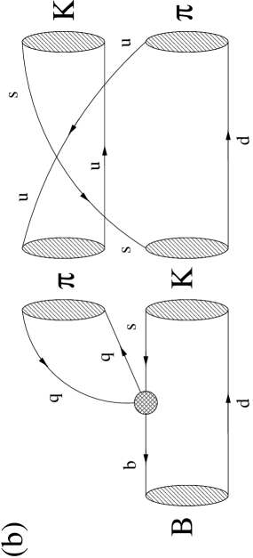
Figure 12: Contributions to the amplitude $T$ through rescattering processes of the kind $B^{0}_{d}\to\{\pi^{-}K^{+}\}\to\pi^{-}K^{+}$ and $B^{0}_{d}\to\{\pi^{0}K^{0}\}\to\pi^{-}K^{+}$. The shaded circles represent insertions of the current–current operators $Q_{1,2}^{q}$, where $q\in\{u,d\}$. In the case of the annihilation topology (c), only the $Q_{1,2}^{d}$ operators contribute.

While the short-distance contributions to the term in curly brackets in (69) cancel, this is not the case for the long-distance contributions associated with final-state interactions. In Fig. 12 we show some of the corresponding Feynman diagrams, where (a) and (b) represent insertions of the current–current operators $Q_{1,2}^{q}$ ($q\in\{u,d\}$) into penguin-like topologies, whereas (c) is an annihilation topology involving only $Q_{1,2}^{d}$. Having a look at these diagrams, it is obvious that their contributions do not in general cancel in (69). Concerning the topologies (a), the $Q_{1,2}^{u}$ operators contribute through rescattering processes of the type $B^{0}_{d}\to\{\pi^{-}K^{+}\}\to\pi^{-}K^{+}$, while the $Q_{1,2}^{d}$ operators contribute through $B^{0}_{d}\to\{\pi^{0}K^{0}\}\to\pi^{-}K^{+}$ and involve the $\bar{d}\,d/\sqrt{2}$ piece of a neutral pion. In the latter case, also $B^{0}_{d}\to\{\eta\,K^{0},\ldots\}\to\pi^{-}K^{+}$ processes are expected to play an important role. In the case of the topologies (b), only rescattering processes of the kind $B^{0}_{d}\to\{\pi^{0}K^{0}\}\to\pi^{-}K^{+}$ contribute. Since $\bar{u}\,u$ and $\bar{d}\,d$ enter in the $\pi^{0}$ wave function with opposite signs, the topologies (b) with $Q_{1,2}^{u}$ and $Q_{1,2}^{d}$ insertions have opposite signs as well and do not cancel in the difference in (69). The annihilation topology (c) has anyway no counterpart with $Q_{1,2}^{u}$ insertions. Consequently, the rescattering contributions to the term in curly brackets in (69) do not cancel. If they are of the same order of magnitude as $\tilde{\cal T}$ describing the strength of the “first step” in the rescattering processes of the type (a) – such a scenario is found in the model calculation performed in [16] – the value of $r$ could in principle be shifted significantly from its “factorized” value (29).

The feature described in the previous paragraph provides an interesting mechanism to generate values of $r$ larger than those obtained within the framework of “factorization”, and may be the reason for the fact that the values of $r$ preferred by present CLEO data are at the edge of compatibility with (29), as we noted in Subsection 3.2. In particular, the small central value of $R=0.65$ may indicate already that $r$ is enhanced considerably by final-state interactions, and it may well be possible that future measurements will stabilize around this naïvely small value.

Although this is good news for the bounds on $\gamma$ from $B\to\pi K$ decays, it is bad news for the corresponding extractions of this CKM angle, which require the knowledge of $r$. Unfortunately, in the case of this quantity, final-state interactions cannot be taken into account in a simple way. Consequently, expectations based on factorization that a future theoretical uncertainty of $r$ as small as ${\cal O}(10\%)$ may be achievable [2, 3] appear too optimistic. If we look, however, at Figs. 10 and 11, we observe that the dependence of $\gamma$ on $r$ is very weak for $r\mathrel{\hbox{\hbox to0.0pt{\hbox{\lower 4.0pt\hbox{$\sim$}}\hss}\hbox{$>$}}}0.3$ in this example; even for values of $R$ as large as 0.85, a significant region around $\gamma=90^{\circ}$ could be excluded. The power of a future accurate measurement of the decays $B^{\pm}\to\pi^{\pm}K$ and $B_{d}\to\pi^{\mp}K^{\pm}$ is therefore probably not a “precision” measurement of $\gamma$, but phenomenologically interesting constraints on this CKM angle.

5 The Role of Electroweak Penguins

Let us begin our discussion of electroweak penguin effects by first having a look at (40). For $\rho=0$, i.e. neglected rescattering effects, the modification of $R_{\rm min}$ through electroweak penguins is described by $\kappa=1+2\,\epsilon\,\cos\Delta+\epsilon^{2}$. These effects are minimal and only of second order in $\epsilon$ for $\Delta\in\{90^{\circ},270^{\circ}\}$, and maximal for $\Delta\in\{0^{\circ},180^{\circ}\}$. In the case of $\Delta=0^{\circ}$, the bounds on $\gamma$ get stronger, excluding a larger region around $\gamma=90^{\circ}$, while they are weakened for $\Delta=180^{\circ}$. In Figs. 13 and 14 we show the maximal electroweak penguin effects for various values of $\epsilon$. The electroweak penguins are “colour-suppressed” in the case of $B^{+}\to\pi^{+}K^{0}$ and $B^{0}_{d}\to\pi^{-}K^{+}$, and estimates based on simple calculations performed at the perturbative quark level, where the relevant hadronic matrix elements are treated within the “factorization” approach, typically give $\epsilon={\cal O}(1\%)$ [8]. Even for such small values of $\epsilon$, there is a sizeable shift of $R_{\rm min}$, as can be seen in Figs. 13 and 14. Comparing these figures with Fig. 4, we observe that $R_{\rm min}$ is more sensitive to electroweak penguin than to rescattering effects. Since the crude estimates yielding $\epsilon={\cal O}(1\%)$ may well underestimate the role of electroweak penguins [2, 15, 21], an improved theoretical description of these topologies is highly desirable.

5.1 An Improved Theoretical Description

Figure 13: The effect of electroweak penguins on $R_{\rm min}$ for $A_{0}=0$. The curves for a given value of $\epsilon$ correspond to $\Delta\in\{0^{\circ},180^{\circ}\}$ and represent the maximal shift from $\epsilon=0$.

Figure 14: The effect of electroweak penguins on $R_{\rm min}$ for $|A_{0}|=0.2$. The curves for a given value of $\epsilon$ correspond to $\Delta\in\{0^{\circ},180^{\circ}\}$ and represent the maximal shift from $\epsilon=0$.

The relevant electroweak penguin amplitude affecting bounds and extractions of the CKM angle $\gamma$ from $B^{\pm}\to\pi^{\pm}K$, $B_{d}\to\pi^{\mp}K^{\pm}$ decays has been given in (21), where $P_{\rm ew}^{t}$ and $\tilde{P}_{\rm ew}^{t}$ correspond to electroweak penguins with internal top quarks and can be expressed in terms of hadronic matrix elements of four-quark operators as follows (see (68)):

$$P_{\rm ew}^{t} = -\,\frac{G_{\rm F}}{\sqrt{2}}\sum_{k=7}^{10}C_{k}(\mu)\langle K^{0}\pi^{+}|Q_{k}(\mu)|B^{+}\rangle$$ (70)

$$\tilde{P}_{\rm ew}^{t} = \frac{G_{\rm F}}{\sqrt{2}}\sum_{k=7}^{10}C_{k}(\mu)\langle K^{+}\pi^{-}|Q_{k}(\mu)|B^{0}_{d}\rangle.$$ (71)

The electroweak penguin operators $Q_{7}$,…,$Q_{10}$ have the following structure:

$$Q_{k}=\frac{3}{2}\sum_{q=u,d,c,s,b}c_{q}\,Q_{k}^{q}\,,$$ (72)

where $c_{q}$ denotes the electrical quark charges and the four-quark operators are given by

$$Q_{7}^{q}=(\bar{b}_{\alpha}s_{\alpha})_{{\rm V-A}}(\bar{q}_{\beta}q_{\beta})_{{\rm V+A}}\,,\quad Q_{8}^{q}=(\bar{b}_{\alpha}s_{\beta})_{{\rm V-A}}(\bar{q}_{\beta}q_{\alpha})_{{\rm V+A}}$$ (73)

$$~{}~{}Q_{9}^{q}=(\bar{b}_{\alpha}s_{\alpha})_{{\rm V-A}}(\bar{q}_{\beta}q_{\beta})_{{\rm V-A}}\,,\quad Q_{10}^{q}=(\bar{b}_{\alpha}s_{\beta})_{{\rm V-A}}(\bar{q}_{\beta}q_{\alpha})_{{\rm V-A}}\,.$$ (74)

The amplitude $P_{\rm ew}^{t}$ can therefore be written as

$$P_{\rm ew}^{t}=-\,\frac{G_{\rm F}}{\sqrt{2}}\,\frac{3}{2}\left[c_{d}\sum_{k=7}^{10}C_{k}(\mu)\langle K^{0}\pi^{+}|Q_{k}^{d}(\mu)|B^{+}\rangle_{\rm T}+c_{d}\sum_{k=7}^{10}C_{k}(\mu)\langle K^{0}\pi^{+}|Q_{k}^{d}(\mu)|B^{+}\rangle_{\rm P}~{}~{}\right.$$ (75)

$$\left.+\,c_{u}\sum_{k=7}^{10}C_{k}(\mu)\langle K^{0}\pi^{+}|Q_{k}^{u}(\mu)|B^{+}\rangle\,+\sum_{q=c,s,b}c_{q}\left\{\sum_{k=7}^{10}C_{k}(\mu)\langle K^{0}\pi^{+}|Q_{k}^{q}(\mu)|B^{+}\rangle\right\}\right].$$

The notation in this expression is as in (69). While the first term describes the contributions of $Q_{k}^{d}$ arising from insertions into tree-diagram-like topologies, the other terms contain in particular also rescattering effects, which may play an important role. Applying the $SU(2)$ isospin symmetry to the hadronic matrix elements of the $Q_{k}^{q}$ operators, we obtain

$$P_{\rm ew}^{t}=\frac{G_{\rm F}}{\sqrt{2}}\,\frac{3}{2}\left[c_{d}\sum_{k=7}^{10}C_{k}(\mu)\langle K^{+}\pi^{-}|Q_{k}^{u}(\mu)|B^{0}_{d}\rangle_{\rm T}+c_{d}\sum_{k=7}^{10}C_{k}(\mu)\langle K^{+}\pi^{-}|Q_{k}^{u}(\mu)|B^{0}_{d}\rangle_{\rm P}~{}~{}\right.$$ (76)

$$\left.+\,c_{u}\sum_{k=7}^{10}C_{k}(\mu)\langle K^{+}\pi^{-}|Q_{k}^{d}(\mu)|B^{0}_{d}\rangle\,+\sum_{q=c,s,b}c_{q}\left\{\sum_{k=7}^{10}C_{k}(\mu)\langle K^{+}\pi^{-}|Q_{k}^{q}(\mu)|B^{0}_{d}\rangle\right\}\right],$$

while we have on the other hand

$$\tilde{P}_{\rm ew}^{t}=\frac{G_{\rm F}}{\sqrt{2}}\,\frac{3}{2}\left[c_{u}\sum_{k=7}^{10}C_{k}(\mu)\langle K^{+}\pi^{-}|Q_{k}^{u}(\mu)|B^{0}_{d}\rangle_{\rm T}+c_{u}\sum_{k=7}^{10}C_{k}(\mu)\langle K^{+}\pi^{-}|Q_{k}^{u}(\mu)|B^{0}_{d}\rangle_{\rm P}~{}~{}\right.$$ (77)

$$\left.+\,c_{d}\sum_{k=7}^{10}C_{k}(\mu)\langle K^{+}\pi^{-}|Q_{k}^{d}(\mu)|B^{0}_{d}\rangle\,+\sum_{q=c,s,b}c_{q}\left\{\sum_{k=7}^{10}C_{k}(\mu)\langle K^{+}\pi^{-}|Q_{k}^{q}(\mu)|B^{0}_{d}\rangle\right\}\right].$$

Concerning the quantity $P_{\rm ew}$, only the difference of these amplitudes is relevant, which is given by

$$\tilde{P}_{\rm ew}^{t}-P_{\rm ew}^{t}=\left(c_{u}-c_{d}\right)\frac{G_{\rm F}}{\sqrt{2}}\,\frac{3}{2}\left[\sum_{k=7}^{10}C_{k}(\mu)\langle K^{+}\pi^{-}|Q_{k}^{u}(\mu)|B^{0}_{d}\rangle_{\rm T}\right.$$ (78)

$$\left.+\,\sum_{k=7}^{10}C_{k}(\mu)\left\{\langle K^{+}\pi^{-}|Q_{k}^{u}(\mu)|B^{0}_{d}\rangle_{\rm P}-\langle K^{+}\pi^{-}|Q_{k}^{d}(\mu)|B^{0}_{d}\rangle\right\}\right].$$

This expression is much simpler than (76) and (77), since the contributions of $Q_{k}^{q}$ with $q=c,s,b$ – including also rescattering contributions that are very hard to estimate – cancel fortunately because of the isospin symmetry. Since only the Wilson coefficients $C_{9}$ and $C_{10}$ are sizeable [30], where $C_{9}$ plays the most important role and is about three times larger than $C_{10}$, the amplitude difference (78) simplifies further and we have only to care about $Q_{9,10}^{u}$ and $Q_{9,10}^{d}$. If we compare these operators with the current–current operators given in (16), we observe that they are related to each other through a simple Fierz transformation:

$$\left.Q_{9}^{u,d}\right|_{\rm Fierz}=\,Q_{1}^{u,d},\quad\left.Q_{10}^{u,d}\right|_{\rm Fierz}=\,Q_{2}^{u,d}.$$ (79)

Beyond the leading order, one has to be careful, when performing such Fierz transformations, since the next-to-leading order Wilson coefficients depend also on the chosen operator basis [30]. Here we will only use leading-order Wilson coefficients for simplicity, and will comment on the influence of next-to-leading order corrections on our “final” result below.

The amplitudes $P_{\rm ew}^{c}$ and $\tilde{P}_{\rm ew}^{c}$ in (21) corresponding to electroweak penguins with internal charm quarks, which would be needed for a consistent use of next-to-leading order Wilson coefficients [30], play a negligible role. The point is that electroweak penguins only become important because of the large top-quark mass, which compensates their suppression relative to the QCD penguins due to the small ratio $\alpha/\alpha_{s}={\cal O}(10^{-2})$ of the QED and QCD couplings. This feature is reflected by the sizeable value of $C_{9}$.

Consequently we arrive at the following expression for $P_{\rm ew}$:

$$P_{\rm ew} = -\lambda^{2}A\,\frac{G_{\rm F}}{\sqrt{2}}\,\frac{3}{2}\,\biggl{[}C_{9}(\mu)\langle K^{+}\pi^{-}|Q_{1}^{u}(\mu)|B^{0}_{d}\rangle_{\rm T}+C_{10}(\mu)\langle K^{+}\pi^{-}|Q_{2}^{u}(\mu)|B^{0}_{d}\rangle_{\rm T}$$ (80)

$$~{}~{}+\left\{C_{9}(\mu)\langle K^{+}\pi^{-}|Q_{1}^{u}(\mu)|B^{0}_{d}\rangle_{\rm P}+C_{10}(\mu)\langle K^{+}\pi^{-}|Q_{2}^{u}(\mu)|B^{0}_{d}\rangle_{\rm P}\right.$$

$$\left.~{}~{}-C_{9}(\mu)\langle K^{+}\pi^{-}|Q_{1}^{d}(\mu)|B^{0}_{d}\rangle-C_{10}(\mu)\langle K^{+}\pi^{-}|Q_{2}^{d}(\mu)|B^{0}_{d}\rangle\right\}\biggr{]},$$

where we have neglected the ${\cal O}(\lambda^{4})$ term in (21) and have used in addition $c_{u}-c_{d}=1$. Remarkably, (80) is completely analogous to the operator expression for $T$ given in (69). Introducing the following non-perturbative “bag” parameters:

$$\frac{1}{3}B_{1}(\mu)\langle K^{+}\pi^{-}|Q_{2}^{u}|B^{0}_{d}\rangle_{\rm T}^{\rm fact}$$ (81)

$$~{}~{}~{}~{}\equiv\langle K^{+}\pi^{-}|Q_{1}^{u}(\mu)|B^{0}_{d}\rangle_{\rm T}+\left\{\langle K^{+}\pi^{-}|Q_{1}^{u}(\mu)|B^{0}_{d}\rangle_{\rm P}-\langle K^{+}\pi^{-}|Q_{1}^{d}(\mu)|B^{0}_{d}\rangle\right\}$$

$$B_{2}(\mu)\langle K^{+}\pi^{-}|Q_{2}^{u}|B^{0}_{d}\rangle_{\rm T}^{\rm fact}$$ (82)

$$~{}~{}~{}~{}\equiv\langle K^{+}\pi^{-}|Q_{2}^{u}(\mu)|B^{0}_{d}\rangle_{\rm T}+\left\{\langle K^{+}\pi^{-}|Q_{2}^{u}(\mu)|B^{0}_{d}\rangle_{\rm P}-\langle K^{+}\pi^{-}|Q_{2}^{d}(\mu)|B^{0}_{d}\rangle\right\},$$

we get

$$\frac{\epsilon}{r}\,e^{i(\Delta-\delta)}=-\,\frac{3}{2\lambda^{2}R_{b}}\left[\frac{C_{9}(\mu)B_{1}(\mu)+3\,C_{10}(\mu)B_{2}(\mu)}{C_{1}^{\prime}(\mu)B_{1}(\mu)+3\,C_{2}^{\prime}(\mu)B_{2}(\mu)}\right],$$ (83)

where also the tiny electroweak penguin contributions to $T$, which have been neglected for simplicity in (69), are included through

$$C_{1}^{\prime}(\mu)\equiv C_{1}(\mu)+\frac{3}{2}\,C_{9}(\mu)\,,\quad C_{2}^{\prime}(\mu)\equiv C_{2}(\mu)+\frac{3}{2}\,C_{10}(\mu)\,.$$ (84)

The expression (83) depends only on a single non-perturbative parameter given by $B_{2}(\mu)/B_{1}(\mu)$, which is in general a complex quantity owing to final-state interactions. It is possible to rewrite (83) in an even more transparent way by using the quantities

$$a_{1}^{\rm eff} \equiv \frac{1}{3}\,C_{1}^{\prime}(\mu)\,B_{1}(\mu)+C_{2}^{\prime}(\mu)\,B_{2}(\mu)$$ (85)

$$a_{2}^{\rm eff} \equiv C_{1}^{\prime}(\mu)\,B_{2}(\mu)+\frac{1}{3}\,C_{2}^{\prime}(\mu)\,B_{1}(\mu)\,,$$ (86)

which correspond to the usual phenomenological colour factors $a_{1}$ and $a_{2}$ describing the intrinsic strength of colour-suppressed and colour-allowed decay processes, respectively [24]. Comparing experimental data on $B^{-}\to D^{(\ast)0}\pi^{-}$ and $\overline{B^{0}_{d}}\to D^{(\ast)+}\pi^{-}$, as well as on $B^{-}\to D^{(\ast)0}\rho^{-}$ and $\overline{B^{0}_{d}}\to D^{(\ast)+}\rho^{-}$ decays gives $a_{2}/a_{1}=0.26\pm 0.05\pm 0.09$ [31], where $a_{1}$ and $a_{2}$ are real quantities and their relative sign is interestingly found to be positive, which is in contrast to the case of $D$ decays.

A straightforward calculation yields

$$B(\mu)\equiv\frac{B_{2}(\mu)}{B_{1}(\mu)}=\frac{1}{3}\left[\frac{a\,e^{i\omega}\,C_{1}(\mu)-C_{2}(\mu)}{C_{1}(\mu)-a\,e^{i\omega}\,C_{2}(\mu)}\right],$$ (87)

where

$$a\,e^{i\omega}\equiv\frac{a_{2}^{\rm eff}}{a_{1}^{\rm eff}}$$ (88)

is in general also a complex quantity ($a=|a_{2}^{\rm eff}|/|a_{1}^{\rm eff}|$ is, however, real and positive). Inserting this expression for $B(\mu)$ into (83), we obtain

$$\frac{\epsilon}{r}\,e^{i(\Delta-\delta)}=\frac{3}{2\lambda^{2}R_{b}}\left[\frac{C_{1}^{\prime}(\mu)C_{9}(\mu)-C_{2}^{\prime}(\mu)C_{10}(\mu)}{C_{2}^{\prime 2}(\mu)-C_{1}^{\prime 2}(\mu)}+a\,e^{i\omega}\left\{\frac{C_{1}^{\prime}(\mu)C_{10}(\mu)-C_{2}^{\prime}(\mu)C_{9}(\mu)}{C_{2}^{\prime 2}(\mu)-C_{1}^{\prime 2}(\mu)}\right\}\right].$$ (89)

Since there is a strong cancellation in the first term, leading to

$$\frac{C_{1}^{\prime}(\mu)C_{9}(\mu)-C_{2}^{\prime}(\mu)C_{10}(\mu)}{C_{1}^{\prime}(\mu)C_{10}(\mu)-C_{2}^{\prime}(\mu)C_{9}(\mu)}={\cal O}(10^{-2})\,,$$ (90)

we finally arrive at

$$\frac{\epsilon}{r}\,e^{i(\Delta-\delta)}\approx\frac{3}{2\lambda^{2}R_{b}}\left[\frac{C_{1}^{\prime}(\mu)C_{10}(\mu)-C_{2}^{\prime}(\mu)C_{9}(\mu)}{C_{2}^{\prime 2}(\mu)-C_{1}^{\prime 2}(\mu)}\right]a\,e^{i\omega}\approx 0.75\times a\,e^{i\omega}\,.$$ (91)

The combination of Wilson coefficients in this expressions is essentially renormalization-scale-independent and changes only by ${\cal O}(1\%)$ when evolving from $\mu=M_{W}$ down to $\mu=m_{b}$. Employing $R_{b}=0.36$ and the leading-order Wilson coefficients

$$C_{1}(m_{b})=-\,0.308,\,\,\,C_{2}(m_{b})=1.144,\,\,\,C_{9}(m_{b})/\alpha=-\,1.280,\,\,\,C_{10}(m_{b})/\alpha=0.328$$ (92)

obtained for $\Lambda_{\overline{{\rm MS}}}=225\,\mbox{MeV}$, we get the numerical value of 0.75 in (91), which we will apply throughout this section. The use of next-to-leading order Wilson coefficients would change this result by only a few per cent. In view of the approximations made to derive (91) – neglect of contributions from $Q_{7}$, $Q_{8}$ and electroweak penguins with internal charm quarks – it is therefore appropriate to use leading-order Wilson coefficients.

The “factorization” approach (corresponding to $B(\mu_{\rm F})=1$ in (83), where $\mu_{\rm F}$ is the “factorization scale”) gives on the other hand

$$\left.\frac{\epsilon}{r}\,e^{i(\Delta-\delta)}\right|_{\rm fact}=\,0.06\,,$$ (93)

which is smaller than (91) for $a\,e^{i\omega}=0.25$ (corresponding to $B(m_{b})\approx 2/3$) by a factor of 3. For $\left.r\right|_{\rm fact}=0.16$ (see (29)), we would have $\left.\epsilon\right|_{\rm fact}=0.01$, which is in accordance with the estimate given in [8].

The expression (91) for the electroweak penguin contribution to the $B\to\pi K$ amplitude relations (18) and (19) shows that the usual terminology of “colour-suppressed” electroweak penguins in this context is justified, since $P_{\rm ew}$ is proportional to the generalized “colour factor” $a_{2}^{\rm eff}$.

5.2 The Decay $B^{\pm}\to\pi^{\pm}\pi^{0}$: A First Step Towards Constraining the Electroweak Penguin Uncertainty

As we have noted above, a comparison of colour-suppressed and colour-allowed $B\to D^{(\ast)}\pi(\rho)$ decays shows that the corresponding value of $a_{2}/a_{1}$ is positive and of ${\cal O}(0.25)$. In the case of $B$-meson decays into $\pi\,K$ or $\pi\,\pi$ final states, the situation concerning “colour-suppression” may, however, be quite different. At present there are unfortunately no experimental data available to investigate this issue. A first step towards achieving this goal, thereby obtaining insights into the importance of the colour-suppressed electroweak penguin amplitude $P_{\rm ew}$ in (19), is provided by the $\bar{b}\to\bar{u}\,u\,\bar{d}$ decay $B^{+}\to\pi^{+}\pi^{0}$. This mode receives only tiny electroweak penguin contributions [20]. Moreover, QCD penguins do not contribute because of the $SU(2)$ isospin symmetry, so that the decay amplitude takes the simple form

$$A(B^{+}\to\pi^{+}\pi^{0})=-\,\frac{1}{\sqrt{2}}\left[T^{(d)}+C^{(d)}\right]=-\,\frac{e^{i\gamma}}{\sqrt{2}}\left[|T^{(d)}|\,e^{i\delta_{T}^{(d)}}+|C^{(d)}|\,e^{i\delta_{C}^{(d)}}\right],$$ (94)

where $T^{(d)}$ and $C^{(d)}$ are usually referred to as colour-allowed and colour-suppressed “tree” amplitudes. Using the $SU(3)$ flavour symmetry, we have

$$|T^{(d)}|=\frac{f_{\pi}}{\lambda\,f_{K}}\,\lambda^{4}A\,R_{b}\,|\tilde{\cal T}|\,,$$ (95)

where $\tilde{\cal T}$ has been introduced in (20), and $f_{\pi}$ and $f_{K}$ denote the pion and kaon decay constants, respectively, taking into account factorizable $SU(3)$ breaking. Introducing

$$a_{\pi\pi}\,e^{i\,\omega_{\pi\pi}}\equiv\frac{C^{(d)}}{T^{(d)}}\,,$$ (96)

we find

$$1+2\,a_{\pi\pi}\,\cos\omega_{\pi\pi}+a_{\pi\pi}^{2}\,=\,\left(\frac{1}{\tilde{r}}\,\frac{\lambda\,f_{K}}{f_{\pi}}\right)^{2}\frac{2\,\mbox{BR}(B^{\pm}\to\pi^{\pm}\pi^{0})}{\mbox{BR}(B^{\pm}\to\pi^{\pm}K)}$$ (97)

and get a lower bound on $a_{\pi\pi}$:

$$a_{\pi\pi}\,\geq\,\left|\,1-\frac{1}{\tilde{r}}\,\frac{\lambda\,f_{K}}{f_{\pi}}\,\sqrt{\frac{2\,\mbox{BR}(B^{\pm}\to\pi^{\pm}\pi^{0})}{\mbox{BR}(B^{\pm}\to\pi^{\pm}K)}}\,\right|,$$ (98)

and an upper limit for $|\sin\omega_{\pi\pi}|$:

$$|\sin\omega_{\pi\pi}|\,\leq\,\frac{1}{\tilde{r}}\,\frac{\lambda\,f_{K}}{f_{\pi}}\,\sqrt{\frac{2\,\mbox{BR}(B^{\pm}\to\pi^{\pm}\pi^{0})}{\mbox{BR}(B^{\pm}\to\pi^{\pm}K)}}\,,$$ (99)

where $\tilde{r}$ corresponds to $\tilde{\cal T}$ and has been defined in (47). At present there is only an upper bound on the combined branching ratio for $B^{\pm}\to\pi^{\pm}\pi^{0}$ available from CLEO [7], which is given by BR$(B^{\pm}\to\pi^{\pm}\pi^{0})<2.0\times 10^{-5}$ and is unfortunately too weak to constrain $a_{\pi\pi}$ and $\omega_{\pi\pi}$ in a meaningful way.

Making use once more of the $SU(3)$ flavour symmetry, we get

$$a\,e^{i\omega}\approx$$

$$\frac{a_{2}^{\pi\pi}+\left[\sum\limits_{k=1}^{2}C_{k}(\mu)\left\{\langle K^{+}\pi^{-}|Q_{3-k}^{u}(\mu)|B^{0}_{d}\rangle_{\rm P}-\langle K^{+}\pi^{-}|Q_{3-k}^{d}(\mu)|B^{0}_{d}\rangle\right\}\right]/\langle K^{+}\pi^{-}|Q_{2}^{u}|B^{0}_{d}\rangle_{\rm T}^{\rm fact}}{a_{1}^{\pi\pi}+\left[\sum\limits_{k=1}^{2}C_{k}(\mu)\left\{\langle K^{+}\pi^{-}|Q_{k}^{u}(\mu)|B^{0}_{d}\rangle_{\rm P}-\langle K^{+}\pi^{-}|Q_{k}^{d}(\mu)|B^{0}_{d}\rangle\right\}\right]/\langle K^{+}\pi^{-}|Q_{2}^{u}|B^{0}_{d}\rangle_{\rm T}^{\rm fact}}$$

with $a_{2}^{\pi\pi}/a_{1}^{\pi\pi}=a_{\pi\pi}\,e^{i\omega_{\pi\pi}}$. This equation can easily be rewritten as

$$a\,e^{i\omega}\approx\left(\frac{1+a_{2}^{\rm res}/a_{2}^{\pi\pi}\,{\cal M}_{\rm res}}{1+{\cal M}_{\rm res}}\right)a_{\pi\pi}\,e^{i\omega_{\pi\pi}},$$ (101)

where we have expressed the terms in the denominator and numerator of (5.2) related to rescattering processes as $a_{1}^{\pi\pi}{\cal M}_{\rm res}$ and $a_{2}^{\rm res}{\cal M}_{\rm res}$, respectively. In general these rescattering contributions preclude a relation of $a_{\pi\pi}\,e^{i\omega_{\pi\pi}}$ to $a\,e^{i\omega}$. However, the rescattering contributions from the $Q_{1}^{u,d}$ current–current operators are disfavoured with respect to those from $Q_{2}^{u,d}$ because of their colour structure. This feature is described by the colour-suppression factor $a_{2}^{\rm res}$ in (101). If this quantity should have the same order of magnitude as $a_{2}^{\pi\pi}$, we would have $a\,e^{i\omega}\approx a_{\pi\pi}\,e^{i\omega_{\pi\pi}}$ not only in the case of tiny rescattering effects, i.e. $|{\cal M}_{\rm res}|\ll 1$, but also for large rescattering contributions. It is interesting to note that we would have $a\,e^{i\omega}\approx C_{1}(m_{b})/C_{2}(m_{b})\approx-\,0.25$, if the rescattering processes from $Q_{2}^{u,d}$ should play a dominant role.

Combining these considerations, we conclude that BR$(B^{\pm}\to\pi^{\pm}\pi^{0})$ is interesting to obtain a lower bound on the electroweak penguin contributions (see (91) and (98)), or to eliminate either $\omega$ or $a$ (see (97)). This strategy – using ironically $B^{+}\to\pi^{+}\pi^{0}$, a decay where electroweak penguins play a very minor role – can be considered as a first step towards constraining the electroweak penguin amplitude $P_{\rm ew}$ in the $B\to\pi K$ relations (18) and (19). Its theoretical accuracy is limited by $SU(3)$-breaking corrections, which may be significant in the case of colour-suppressed topologies, and by rescattering effects. In the numerical examples given in the following subsection, we assume $a={\cal O}(0.25)$, i.e. that the $B\to D^{(\ast)}\pi(\rho)$ and $B\to J/\psi\,K^{(\ast)}$ measurements available at present [31] inform us also about the intrinsic “strength” of colour suppression in $B\to\pi K$ decays, and keep $\omega$ as a free parameter.

5.3 A Closer Look at Electroweak Penguin Effects in Strategies to Constrain and Determine $\gamma$

Since (91) implies a correlation between $\epsilon$ and $r$ described by

$$\epsilon=q\,r\,,\quad\Delta=\delta+\omega\,,$$ (102)

where $q\approx 0.75\times a$, (30) is modified. Using (102) to replace $\epsilon$ and $\Delta$ in (25), we get

$$R=1-\frac{2\,r}{w}\left(\tilde{h}\cos\delta+\tilde{k}\sin\delta\right)+v^{2}r^{2},$$ (103)

with

$$v=\sqrt{1-2\,q\,\cos\omega\cos\gamma+q^{2}}$$ (104)

and

$$\tilde{h} = \cos\gamma+\rho\cos\theta-q\left[\,\cos\omega+\rho\cos(\theta-\omega)\cos\gamma\,\right]$$ (105)

$$\tilde{k} = \rho\sin\theta+q\left[\,\sin\omega-\rho\sin(\theta-\omega)\cos\gamma\,\right].$$ (106)

If we keep both $r$ and the strong phase $\delta$ as free parameters in (103), we find that $R$ takes the following minimal value:

$$R_{\rm min}=\left[\frac{1+2\,q\,\rho\,\cos(\theta+\omega)+q^{2}\rho^{2}}{\left(1-2\,q\,\cos\omega\cos\gamma+q^{2}\right)\left(1+2\,\rho\,\cos\theta\cos\gamma+\rho^{2}\right)}\right]\sin^{2}\gamma\,,$$ (107)

which simplifies to $R_{\rm min}=(\sin^{2}\gamma)/(1-2\,q\,\cos\omega\cos\gamma+q^{2})$ for $\rho=0$, i.e. in the case of neglected rescattering effects. In Fig. 15 we have illustrated the latter expression for various values of $a$. The curves shifted to the left correspond to $\omega=0^{\circ}$, while those shifted to the right correspond to $\omega=180^{\circ}$ and represent the maximal electroweak penguin effects for a given value of $a$. For $|\omega|=90^{\circ}$, these effects are minimal and only of second order in $a$.

Figure 15: The effect of electroweak penguins on $R_{\rm min}$ described by (107). The curves for a given value of $a$ (except the dot-dashed line) correspond to $\omega\in\{0^{\circ},180^{\circ}\}$.

As was pointed out in Subsection 3.1, the strong phase $\delta$ in (103) can be eliminated with the help of the pseudo-asymmetry $A_{0}$. The modification of (31) through (102) is as follows:

$$\tilde{A}=\tilde{B}\sin\delta-\tilde{C}\cos\delta\,,$$ (108)

where

$$\tilde{A}=\frac{w}{r}\left[\,\frac{A_{0}-A_{+}}{2\sin\gamma}+q\,r^{2}\sin\omega\,\right],\,\,\,\,\tilde{B}=1+q\,\rho\,\cos(\theta-\omega)\,,\,\,\,\,\tilde{C}=q\,\rho\,\sin(\theta-\omega)\,,$$ (109)

and gives

$$R=L+M\,r^{2}\mp\sqrt{-\,N\,r^{4}+2\,P\,r^{2}-Q}\,,$$ (110)

with

$$L=1-\left(\frac{A_{0}-A_{+}}{2\sin\gamma}\right)\tilde{D}\,,\,\,\,\,M=v^{2}-\tilde{D}\,q\,\sin\omega\,,\,\,\,\,N=(\tilde{E}\,q\,\sin\omega)^{2}$$

$$P=\left[\,\frac{\tilde{B}^{2}+\tilde{C}^{2}}{2\,w^{2}}-\left(\frac{A_{0}-A_{+}}{2\,\sin\gamma}\right)\,q\,\sin\omega\,\right]\tilde{E}^{2},\,\,\,\,Q=\left[\left(\frac{A_{0}-A_{+}}{2\sin\gamma}\right)\tilde{E}\right]^{2}$$ (111)

and

$$\tilde{D}=2\left(\frac{\tilde{k}\,\tilde{B}-\tilde{h}\,\tilde{C}}{\tilde{B}^{2}+\tilde{C}^{2}}\right),\,\,\,\,\tilde{E}=2\left(\frac{\tilde{h}\,\tilde{B}+\tilde{k}\,\tilde{C}}{\tilde{B}^{2}+\tilde{C}^{2}}\right).$$ (112)

If we keep $r$ as a free parameter in (110), we find that $R$ takes minimal and maximal values, which are given by

$$R_{\rm min}^{\rm max}=\frac{1}{N}\left[\,LN+MP\pm\sqrt{(P^{2}-NQ)(M^{2}+N)}\,\right]$$ (113)

and correspond to

$$r=r_{\rm min}^{\rm max}\equiv\sqrt{\frac{P}{N}\pm\frac{M}{N}\sqrt{\frac{P^{2}-NQ}{M^{2}+N}}}\,.$$ (114)

Moreover we get the following expression for $r$:

$$r=\sqrt{r_{\rm ext}^{2}+\frac{(R-R_{\rm ext})M\pm\sqrt{(R-R_{\rm ext})\left[\,2\,MP+(2\,L-R-R_{\rm ext})N\,\right]}}{M^{2}+N}}\,,$$ (115)

where “ext” stands for either “min” or “max”, i.e. denotes the extremal values. It is possible to rewrite (113) in a more transparent way as follows:

$$R_{\rm min}^{\rm max}=\frac{1}{2\,(w\,q\,\sin\omega)^{2}}\left[\,v^{2}y\pm\sqrt{(y^{2}-z^{2})(v^{4}-4\,q^{2}\sin^{2}\omega\,\sin^{2}\gamma)}\,\right],$$ (116)

where

$$y=1+2\,q\,\rho\,\cos(\theta+\omega)+q^{2}\rho^{2}-z\,,\quad z=\left(\frac{w^{2}A_{0}}{\sin\gamma}\right)q\,\sin\omega\,.$$ (117)

Concerning phenomenological applications, only the minimal value of $R$ plays an important role, since $R^{\rm max}$ turns out to be much larger than 1.

In the case of two interesting special cases, (116) simplifies considerably. First, for $A_{0}=0$ we have

$$\left.R_{\rm min}\right|_{A_{0}=0}=\frac{2}{v^{2}w^{2}}\left[\frac{1+2\,q\,\rho\cos(\theta+\omega)+q^{2}\rho^{2}}{1+\sqrt{1-\left(2\,q\,\sin\omega\,\sin\gamma/v^{2}\right)^{2}}}\right]\sin^{2}\gamma\,,$$ (118)

which agrees with (107) for $q\,\sin\omega=0$, and gives larger values for $R_{\rm min}$, i.e. stronger bounds on $\gamma$, otherwise. Another important case is $q\,\sin\omega=0$, corresponding to $\omega\in\{0^{\circ},180^{\circ}\}$ for $q\not=0$. In this case, $R_{\rm min}$ takes the same form as (40). The expression for $\kappa$ is, however, very different (and $\cos\omega=\pm 1$):

$$\kappa=\frac{1+2\,q\,\rho\,\cos\theta\,\cos\omega+q^{2}\rho^{2}}{(1-2\,q\,\cos\omega\,\cos\gamma+q^{2})(1+2\,\rho\,\cos\theta\,\cos\gamma+\rho^{2})}\,.$$ (119)

Figure 16: The effect of electroweak penguins described by (91) on $R_{\rm min}$ for $A_{0}=+\,0.2$. Except for the solid and dot-dashed lines, the curves correspond to $\omega\in\{0^{\circ},180^{\circ}\}$.

In Fig. 16 we illustrate the effect of electroweak penguins described by (91) on $R_{\rm min}$ for $A_{0}=+\,0.2$ by using (116) for various values of $a$ and neglected rescattering effects, i.e. $\rho=0$. The curves shifted to the left correspond to $\omega=0^{\circ}$, those shifted to the right to $\omega=180^{\circ}$. In Figs. 17 and 18 we show the corresponding effects in the $\gamma$–$r$ plane for $\omega=0^{\circ}$ and $\pm 90^{\circ}$, respectively. In the latter case, we have chosen $a=0.3$. The contours shown in these figures have been calculated by using (115). The case corresponding to $\omega=180^{\circ}$ can easily be obtained from Fig. 17 by replacing $\gamma\to 180^{\circ}-\gamma$.

Figure 17: The shift of the contours in the $\gamma$–$r$ plane corresponding to $R=0.65$, $|A_{0}|=0.2$ through electroweak penguins described by (91) for $\omega=0^{\circ}$ and $\rho=0$.

Figure 18: The shift of the contours in the $\gamma$–$r$ plane corresponding to $R=0.65$, $A_{0}=0.2$ through electroweak penguins described by (91) for $a=0.3$ and $\rho=0$.

Figure 19: Electroweak penguin and rescattering effects for $R_{\rm min}$ in the case of $|A_{0}|=0.2$ and $|A_{+}|=0.1$ ($\omega\in\{0^{\circ},180^{\circ}\}$).

Figure 20: Electroweak penguin and rescattering effects for $R_{\rm min}$ in the case of $A_{0}=0.2$ and $|A_{+}|=0.1$ ($\omega=\pm 90^{\circ}$).

6 Combined Rescattering and Electroweak Penguin Effects

To end the discussion of rescattering and electroweak penguin effects in strategies to constrain and determine the CKM angle $\gamma$ from $B^{\pm}\to\pi^{\pm}K$ and $B_{d}\to\pi^{\mp}K^{\pm}$ decays, let us illustrate the situation concerning $R_{\rm min}$ in the case of measured asymmetries $|A_{0}|=0.2$ and $|A_{+}|=0.1$. The latter CP asymmetry allows us to obtain a lower bound on $\rho$ and to eliminate the CP-conserving strong phase $\theta$ for a given value of $\rho$, as we discussed in Section 4. In Figs. 19 and 20 we have chosen $\rho=0.15$. The electroweak penguin effects are described in these figures by $a=0.25$ and various values of the strong phase $\omega$. We see that an important difference arises between $\omega=0^{\circ}$ and $\omega=180^{\circ}$.

In the case of large rescattering effects, for example $\rho=0.15$, as shown in Figs. 19 and 20, the branching ratio for the decay $B^{+}\to K^{+}\overline{K^{0}}$ may be enhanced by one order of magnitude from its “short-distance” value ${\cal O}(10^{-6})$ to the $10^{-5}$ level, which should be accessible at future $B$ factories. Using the $SU(3)$ flavour symmetry to relate this mode to $B^{+}\to\pi^{+}K^{0}$, the rescattering effects affecting $R_{\rm min}$ can be controlled completely, as we saw in Subsection 4.3. In particular, following this strategy, no knowledge about $\rho$ would be needed as it was in Figs. 19 and 20.

Although we could derive a transparent expression (see (91)) to describe the electroweak penguin contributions affecting the isospin relations (18) and (19) between $B^{+}\to\pi^{+}K^{0}$ and $B^{0}_{d}\to\pi^{-}K^{+}$, it is more difficult to control them using experimental data if rescattering effects are large. A first step in this direction is provided by the branching ratio for $B^{+}\to\pi^{+}\pi^{0}$, as we have pointed out in Subsection 5.2. In Figs. 19 and 20 we have assumed that $a$ takes a value of $0.25$, which is of the same order of magnitude as the strength of colour suppression in $B\to D^{(\ast)}\pi(\rho)$ and $B\to J/\psi\,K^{(\ast)}$ decays, and have kept $\omega$ as a free CP-conserving strong phase.

At this point we could give more examples to illustrate the possible impact of combined rescattering and electroweak penguin effects on information on the CKM angle $\gamma$ obtained from $B\to\pi K$ decays. Since it is now an easy exercise to play with the corresponding formulae, we will not consider other scenarios in this paper. Hopefully, improved experimental data will be available in the near future, allowing us to go beyond these selected examples and to perform a solid analysis of the corresponding decays.

7 Conclusions

In summary, we have presented a general parametrization of the $B^{+}\to\pi^{+}K^{0}$ and $B^{0}_{d}\to\pi^{-}K^{+}$ decay amplitudes within the framework of the Standard Model in terms of “physical quantities”, taking into account both rescattering and electroweak penguin effects. These decays offer an experimentally feasible way to obtain direct information on the CKM angle $\gamma$ at planned $B$ factories, which will start operating in the near future, and are therefore of particular phenomenological interest. In this respect, the ratio $R$ of their combined branching ratios and the pseudo-asymmetry $A_{0}$ play the key role. As soon as these observables, i.e. the branching ratios for $B^{+}\to\pi^{+}K^{0}$, $B^{0}_{d}\to\pi^{-}K^{+}$ and their charge-conjugates, have been measured, contours in the $\gamma$–$r$ plane can be calculated with the help of the formulae derived in this paper. These contours imply allowed ranges for both $r$ and $\gamma$. For $A_{0}\not=0$, values of $\gamma$ within intervals around $0^{\circ}$ and $180^{\circ}$ can be excluded, and if $R$ should turn out to be smaller than 1, also values around $90^{\circ}$ can be ruled out. In particular the latter case is of particular interest, since the corresponding range for $\gamma$ would then be complementary to its presently allowed range obtained from the usual fits of the unitarity triangle. If $r$ could be fixed by using an additional input, $\gamma$ could not only be constrained, but determined up to a four-fold ambiguity.

In order to derive these bounds and to obtain the contours in the $\gamma$–$r$ plane, isospin symmetry has been used, which is certainly an excellent working assumption. The theoretical cleanliness is, however, limited by certain rescattering and electroweak penguin effects. Our formulae include these contributions in a completely general way, and therefore allow us to investigate the sensitivity to these effects and to take them into account by using additional experimental information.

The rescattering processes may lead to sizeable CP violation in $B^{+}\to\pi^{+}K^{0}$, possibly as large as ${\cal O}(10\%)$. We have pointed out that such CP asymmetries would provide a lower bound on $\rho$, i.e. a first constraint on the strength of the rescattering effects, and are useful to include these final-state interactions in the bounds on $\gamma$. In order to control the rescattering effects in these bounds, $B^{+}\to K^{+}\overline{K^{0}}$ may be a “gold-plated” mode. It can be related to $B^{+}\to\pi^{+}K^{0}$ with the help of the $SU(3)$ flavour symmetry and provides sufficient information not just to constrain, but to take into account the final-state interaction effects in the bounds on $\gamma$ completely. As a by-product, this strategy gives moreover an allowed region for $\rho$, and excludes values of $\gamma$ within ranges around $0^{\circ}$ and $180^{\circ}$. It is interesting to note that $SU(3)$ breaking enters in this approach only at the “next-to-leading order” level, as it represents a correction to the correction to the bounds on $\gamma$ arising from rescattering processes. Moreover this strategy works also if the CP asymmetry in $B^{+}\to\pi^{+}K^{0}$ should turn out to be very small. In this case there may also be large rescattering effects, which would then not be signalled by sizeable CP violation in this channel.

At first sight, an experimental study of $B^{+}\to K^{+}\overline{K^{0}}$ appears to be challenging, since model estimates performed at the perturbative quark level give a combined branching ratio BR$(B^{\pm}\to K^{\pm}K)={\cal O}(10^{-6})$, which is one order of magnitude below the present upper limit obtained by the CLEO collaboration. However, as we have pointed out in this paper, rescattering processes may well enhance this branching ratio by ${\cal O}(10)$, so that it may actually be much closer to the CLEO limit than naïvely expected. Consequently, in the case of large rescattering contributions, i.e. when we have to take them into account in the bounds on $\gamma$, the branching ratio for the decay allowing us to accomplish this task, $B^{+}\to K^{+}\overline{K^{0}}$, may be significantly enhanced through these very rescattering effects, so that this strategy should be feasible at future $B$ factories.

Although the decay $B^{+}\to K^{+}\overline{K^{0}}$ allows us to determine the shift of the contours in the $\gamma$–$r$ plane arising from rescattering processes, it does not allow us to take into account these effects also in the determination of $\gamma$, requiring some knowledge on $r$, in contrast to the $\gamma$ bounds. This quantity is not just the ratio of a “tree” to a “penguin” amplitude, which is the usual terminology in the literature, but has a rather complex structure and may be considerably affected by final-state interactions. Consequently, in the case of large rescattering effects, $r$ is expected to be shifted significantly from its “factorized” value and its theoretical uncertainty is very hard to control. Interestingly, the small present central value $R=0.65$ implies a range for $r$ that is at the edge of compatibility with these “factorized” results and favours larger values of $r$. This feature may already give us a first hint that rescattering effects play in fact an important role, and it may well be that future experimental results for $R$ will stabilize at the 0.65 level. In this case, a measurement of BR$(B^{\pm}\to K^{\pm}K)={\cal O}(10^{-5})$ and large CP violation in this channel would not be a surprise. In the recent literature it has been claimed by some authors that such rescattering processes would spoil the bounds on $\gamma$. It is interesting to note that these effects may actually be responsible for a strong realization of these bounds, i.e. for a small value of $R$, thereby making them phenomenologically relevant.

Concerning electroweak penguins, model calculations using “factorization” to deal with hadronic matrix elements typically give contributions at the $1\%$ level in the case of $B^{+}\to\pi^{+}K^{0}$ and $B^{0}_{d}\to\pi^{-}K^{+}$ decays, where electroweak penguins contribute only in “colour-suppressed” form. In this paper, we have presented an improved theoretical description of the electroweak penguin amplitude affecting the isospin relations between the decay amplitudes of these modes, and have derived a transparent expression, clarifying also the notion of “colour-suppressed” electroweak penguins. Our approach does not use questionable assumptions, such as factorization, and makes use of only the general structure of the electroweak penguin operators and of the isospin symmetry of strong interactions to relate the hadronic matrix elements corresponding to $B^{+}\to\pi^{+}K^{0}$ and $B^{0}_{d}\to\pi^{-}K^{+}$ transitions. We have seen that the importance of electroweak penguins is closely related to the ratio of certain “effective” colour factors $a_{2}^{\rm eff}/a_{1}^{\rm eff}$. Using $|a_{2}^{\rm eff}|/|a_{1}^{\rm eff}|=0.25$ gives an enhancement of the relevant electroweak penguin amplitude by a factor of 3 with respect to the factorized result. A first step towards constraining this electroweak penguin amplitude experimentally is provided by the mode $B^{+}\to\pi^{+}\pi^{0}$. Our formulae include the electroweak penguin contributions in a completely general way, allowing us to take them into account once we have a better understanding of “colour-suppression” and rescattering effects in $B\to\pi K$ decays.

Although the decays $B^{+}\to\pi^{+}K^{0}$, $B^{0}_{d}\to\pi^{-}K^{+}$ and their charge conjugates will probably not allow a precision measurement of $\gamma$, they are expected to provide a very fertile ground to constrain this CKM angle. An accurate measurement of these modes, as well as of $B^{\pm}\to K^{\pm}K$, is therefore an important goal of the future $B$ factories. The corresponding experimental results will certainly be very exciting.

References

- [1] R. Fleischer, Phys. Lett. B365 (1996) 399.
- [2] M. Gronau and J.L. Rosner, CALT-68-2142 (1997) [hep-ph/9711246].
- [3] F. Würthwein and P. Gaidarev, CALT-68-2153 (1997) [hep-ph/9712531].
- [4] The BaBar Physics Book, SLAC-R-504, in preparation.
- [5] L.L. Chau and W.-Y. Keung, Phys. Rev. Lett. 53 (1984) 1802; C. Jarlskog and R. Stora, Phys. Lett. B208 (1988) 268.
- [6] N. Cabibbo, Phys. Rev. Lett. 10 (1963) 531; M. Kobayashi and T. Maskawa, Progr. Theor. Phys. 49 (1973) 652.
- [7] R. Godang et al., CLEO 97-27, CLNS 97/1522 (1997) [hep-ex/9711010].
- [8] R. Fleischer and T. Mannel, Phys. Rev. D57 (1998) 2752.
- [9] A.J. Buras, Technical University Munich preprint TUM-HEP-299-97 (1997) [hep-ph/9711217], invited plenary talk given at the 7th International Symposium on Heavy Flavor Physics, Santa Barbara, California, 7-11 July 1997, to appear in the proceedings.
- [10] Y. Grossman, Y. Nir, S. Plaszczynski and M.-H. Schune, SLAC-PUB-7622 (1997) [hep-ph/9709288].
- [11] L. Wolfenstein, Phys. Rev. D52 (1995) 537; J. Donoghue, E. Golowich, A. Petrov and J. Soares, Phys. Rev. Lett. 77 (1996) 2178.
- [12] B. Blok and I. Halperin, Phys. Lett. B385 (1996) 324; B. Blok, M. Gronau and J.L. Rosner, Phys. Rev. Lett. 78 (1997) 3999.
- [13] A. Buras, R. Fleischer and T. Mannel, CERN-TH/97-307 (1997) [hep-ph/9711262].
- [14] J.-M. Gérard and J. Weyers, Université catholique de Louvain preprint UCL-IPT-97-18 (1997) [hep-ph/9711469].
- [15] M. Neubert, CERN-TH/97-342 (1997) [hep-ph/9712224].
- [16] A.F. Falk, A.L. Kagan, Y. Nir and A.A. Petrov, Johns Hopkins University preprint JHU-TIPAC-97018 (1997) [hep-ph/9712225].
- [17] D. Atwood and A. Soni (1997) [hep-ph/9712287].
- [18] M. Bander, D. Silverman and A. Soni, Phys. Rev. Lett. 43 (1979) 242.
- [19] R. Fleischer, Z. Phys. C58 (1993) 483 and C62 (1994) 81; G. Kramer, W.F. Palmer and H. Simma, Z. Phys. C66 (1995) 429.
- [20] For a recent review, see R. Fleischer, Int. J. Mod. Phys. A12 (1997) 2459.
- [21] R. Fleischer and T. Mannel, University of Karlsruhe preprint TTP97-22 (1997) [hep-ph/9706261].
- [22] L. Wolfenstein, Phys. Rev. Lett. 51 (1983) 1945.
- [23] M. Bauer, B. Stech and M. Wirbel, Z. Phys. C29 (1985) 637 and C34 (1987) 103.
- [24] M. Neubert and B. Stech, CERN-TH/97-99 (1997) [hep-ph/9705292], to appear in Heavy Flavours II, Eds. A.J. Buras and M. Lindner (World Scientific, Singapore, 1998).
- [25] A. Ali and C. Greub, DESY-97-126 (1997) [hep-ph/9707251].
- [26] A.J. Buras and R. Fleischer, Phys. Lett. B341 (1995) 379; R. Fleischer, Phys. Lett. B341 (1994) 205.
- [27] M. Ciuchini, E. Franco, G. Martinelli and L. Silvestrini, Nucl. Phys. B501 (1997) 271; M. Ciuchini, R. Contino, E. Franco, G. Martinelli and L. Silvestrini, CERN-TH/97-188 (1997) [hep-ph/9708222].
- [28] J. Schwinger, Phys. Rev. Lett. 12 (1964) 630; R.P. Feynman, in Symmetries in Particle Physics, Ed. A. Zichichi (Acad. Press, New York, 1965); O. Haan and B. Stech, Nucl. Phys. B22 (1970) 448; D. Fakirov and B. Stech, Nucl. Phys. B133 (1978) 315; L.L. Chau, Phys. Rep. B95 (1983) 1.
- [29] J.D. Bjorken, Nucl. Phys. B (Proc. Suppl.) 11 (1989) 325; SLAC-PUB-5389 (1990), published in the proceedings of the SLAC Summer Institute 1990, p. 167.
- [30] For a review, see G. Buchalla, A.J. Buras and M.E. Lautenbacher, Rev. Mod. Phys. 68 (1996) 1125.
- [31] T.E. Browder, published in the proceedings of the 28th International Conference on High-Energy Physics (ICHEP ’96), Warsaw, Poland, 25–31 July 1996, Eds. Z. Ajduk and A.K. Wroblewski (World Scientific, Singapore, 1997), p. 1139 [hep-ph/9611373].