Università degli Studi di Milano

Facoltà di Scienze Matematiche, Fisiche e Naturali

Dipartimento di Fisica

Ph.D. Thesis

Next-to-Leading-Order Corrections to

the Production of Heavy-Flavour

Jets in $e^{+}e^{-}$ Collisions

Carlo Oleari

1994–1997

Contents

toc

Introduction

Radiative corrections to jet production in $e^{+}e^{-}$ annihilation at order $\alpha_{s}^{2}$ were computed a long time ago [2, 3, 4]. These calculations were, however, performed for massless quarks.

This is sufficient in most practical applications: in fact, if we consider the heaviest quark that can be produced nowadays at LEP, the $b$ quark, we can say that, at relatively low energy, the $b$ fraction is strongly suppressed, and, at high energy (i.e. on the $Z$ peak and beyond), mass effects can be neglected for many observables, because they appear as powers of the ratio of the mass over the total energy.

Nevertheless there are several reasons why a massive next-to-leading-order calculation is desirable.

• First of all, there are quantities, such as the heavy-flavour momentum correlation [5, 6], that, although well defined in the massless limit, cannot be computed using the massless result.

• Secondly, a massive calculation finds application in the area of fragmentation functions, where it can be used to improve the resummed cross section.

• Then, this type of calculation helps to understand the relevance of mass corrections in the determination of $\alpha_{s}$ from event shape variables and jets, and may be used to measure quark masses [7, 8].

• Finally, in the future accelerators, where high energies will be reached (Next Linear Collider), $t\overline{t}$ pairs will be produced and mass effects are very likely to be important in those measurements.

In this thesis, we describe a Next-to-Leading-Order (NLO) calculation of the heavy-flavour production cross section in $e^{+}e^{-}$ collisions, including quark mass effects, for unoriented quantities.

At NLO, we get contributions both from two-, three- and from four-particle final states. The amplitudes describing these contributions contain infrared and ultraviolet divergences. Therefore, some regularization procedure is needed. We use the dimensional regularization, that consists in changing the space dimensions $d$ from $4$ to $4-2\epsilon$. In this way, soft and ultraviolet divergences appear as poles in $\epsilon$. At the end of the calculation, the renormalization procedure takes care of the ultraviolet poles, while the infrared poles must cancel for infrared-safe physical quantities.

Very recently, two calculations have appeared in the literature dealing with the same problem [7]–[10]. They both use a slicing method, in order to deal with infrared divergences. This method consists to exclude, from numerical integration, the region of soft and collinear singularities. For this reason, a cut-off parameter is introduced in the energy region of soft gluons and in the collinear limit. In the excluded phase space regions, the transition amplitudes are replaced by their limiting values and the integration is done analytically, in order to obtain the coefficients of the infrared poles $1/\epsilon$ and $1/\epsilon^{2}$, that must cancel the corresponding terms in the virtual diagrams. Together with the poles, there is a finite part, which is integrated numerically over the remaining three-body phase space. Finally, the full transitions are integrated numerically in $d=4$ dimensions over the four-body phase space, above the energy cut-off. Both results, the semi-analytical and the full-numerical one, depend on the choice for the value of the cut-off. Since this parameter was introduced arbitrarily, the final result must be independent from this value.
The smaller this cut-off is, the better result is obtained: in fact, this is an approximate method, because it substitutes, in the singular region, the exact transition amplitudes with their limiting values. On the other hand, for small cut-off parameters, the numerical integration start to fail since the integration region gets closer and closer to the singular points. The best solution is found in the region of the cut-off values where the computed physical quantities become nearly independent from these values.

In our work, we preferred to use a subtraction method, since, in this way, we do not need to worry about taking the limit for small cut-off parameters. Subtraction methods for the calculation of radiative corrections to $e^{+}e^{-}\,\mbox{$\rightarrow$}\,\mbox{jets}$ have been used in Refs. [2, 11], and they have also been successfully employed in the calculation of hadronic production processes.

Together with the quoted massless calculations, parts of the massive calculation were computed by other groups: in the work of Ref. [12], a calculation of the process $e^{+}e^{-}\,\mbox{$\rightarrow$}\,Q\overline{Q}gg$ is given, but virtual corrections to the process $e^{+}e^{-}\,\mbox{$\rightarrow$}\,Q\overline{Q}g$ are not included. In the same work, the amplitudes for two $Q\overline{Q}$ pairs in the final state are calculated. In Ref. [13], the NLO corrections to the production of a heavy-quark pair plus a photon are given, including both real and virtual contributions, while, in Ref. [14], the virtual contribution with a three-fermion loop is computed.

In this thesis we deal with virtual and real contributions to the $e^{+}e^{-}$ annihilation process, that is with terms coming from the interference between one-loop diagrams with the tree-level terms and with final states characterized by a heavy couple of quarks plus a pair of gluons or light quarks. The computation of these contributions is the really hard part of the full calculation.

This work is organized in a quite reverse order: in fact, we first give two physical applications of our calculation, leaving to the other chapters the detailed description of the full computation.

In Chapter 1, we introduce the heavy-flavour momentum correlation, its relationship with the measurement of $R_{b}$, and the results we have obtained at leading and next-to-leading order. The computation of this quantity was the initial reason that conducted us to perform this calculation.

In Chapter 2, we revisit the fragmentation-function formalism for heavy quarks and the connection with our fixed order calculation. In fact, we check the validity of the initial conditions for the fragmentation functions, the NLO splitting functions in the time-like region and we derive an improved cross section, valid at NLO, for energies of order of the mass, but valid at Next-to-Leading-Log for energies much larger than the mass.

The complete calculation is given in the following chapters: in Chapter 3, we introduce the kinematical variables necessary to describe unoriented quantities, and we find the expression of the phase space in $d=4-2\epsilon$ dimensions for the three-body final state ($Q\overline{Q}g$) and for the four-body final states ($Q\overline{Q}gg$, $Q\overline{Q}q\overline{q}$ and $Q\overline{Q}Q\overline{Q}$).

In Chapter 4, we introduce the notation used during the calculation and we present the Feynman diagrams and the cut-diagrams which contribute to the differential cross section. All the results are in an analytic form and are implemented in a FORTRAN program. This program can compute each sort of unoriented infrared-safe shape variables and jet-clustering algorithms. This chapter is the hard part of the thesis, and some of the calculations involved, together with other details, are given in the appendixes.

The check of the cancellation of the infrared poles is performed in Chapter 5, where we apply the subtraction method. We first give a pedagogical introduction of this method before using it on the full cross section. In this chapter, we show how we can avoid to compute two-loop contributions and how we obtain the limits of the amplitudes in the soft and collinear regime. At the end, we list some controls we have done: both internal consistency and external comparisons with the results of other groups. In fact, we found satisfactory agreement between our jet-clustering results and those of Ref. [7].

In Chapter 6 we present some tables computed with different values of the ratio $m/E$, and we compare these results with the massless case. For this kind of calculations, it would be difficult to perform analytical comparisons: for example, at the moment, this is impossible, since the other two groups [7]–[10] have used a different method of computation. For this reason, we have chosen a few shape variables, and we have computed some moments, which can be obtained with a great precision. In addition, we present the results for the three-jet decay rate, computed according to four jet-clustering algorithms, for different values of the cut parameter.

Finally, we summarize our work in the concluding chapter.

Chapter 1 Momentum correlation

In the early of 1996, the discrepancy between the measured and the theoretical value of $R_{b}$ was drawing considerable attention in the physics community. We then began investigating on a possible systematic error, of dynamical origin, in the measurement of $R_{b}$.

Very soon we realized that our first order result in $\alpha_{s}$ was to be complemented by a second order calculation, so that we started the computation of the differential cross section for the process $e^{+}e^{-}\,\mbox{$\rightarrow$}\,Z/\gamma\,\mbox{$\rightarrow$}\,Q\overline{Q}+X$, where $Q$ is a massive quark, $X$ is anything else, at order $\alpha_{s}^{2}$.

1.1 Momentum correlation in $Z/\gamma\,\mbox{$\rightarrow$}\,b\bar{b}$

$R_{b}$ is defined by the ratio

$$R_{b}=\frac{\displaystyle\Gamma_{b\bar{b}}}{\displaystyle\Gamma_{\rm had}}\;,$$ (1.1)

where $\Gamma$ is the decay width of the $Z/\gamma$ into the specified final state. In several experimental techniques for the measurement of $R_{b}$, the tagging efficiency is extracted from the data by comparing the sample of events in which only one $b$ has been tagged, with the one in which both $b$’s are observed. If the production characteristics of the $b$ and the $\bar{b}$ were completely uncorrelated, this method would yield the exact answer, without need of corrections. Of course, other correlations of experimental nature should be properly accounted for, but their discussion is outside the scope of the present theoretical section. Here we deal with the standard QCD gluon emission, that generates a correlation of the quark-antiquark momenta of order $\alpha_{s}$. Other dynamical effects, like the production of heavy-quark pairs via a gluon-splitting mechanism, may affect the measurement. However, they are, to some extent, better understood: in fact, they tend to give soft heavy quarks, and they are, therefore, easily eliminated.

We begin by considering the simple case in which the efficiency for tagging a $B$ meson is a linear function of its momentum. This simplifying assumption allows us to make very precise statements about the correlation. Furthermore, it is not extremely far from reality, in the sense that the experimental tagging efficiency is often a growing function of the $B$ momentum. For this reason, we introduce two kinematical variables to describe the momentum carried by the couple quark-antiquark

$$\overline{x}_{1(2)}=\frac{|{\bf p}|_{{{\rm\scriptscriptstyle B}}({\rm\scriptscriptstyle\overline{B}})}}{|{\bf p}|^{(\rm max)}_{{\rm\scriptscriptstyle B}}}\;,$$ (1.2)

where ${\bf p}$ denotes the meson three-momentum. In terms of the usual notation, where

$$x_{1(2)}=\frac{2\,E_{{\rm\scriptscriptstyle B}({\rm\scriptscriptstyle\overline{B}})}}{E}\;,$$ (1.3)

with $E$ the total centre-of-mass energy and $E_{{\rm\scriptscriptstyle B}({\rm\scriptscriptstyle\overline{B}})}$ the energy of the $B(\overline{B})$ meson, we have

$$\overline{x}_{1(2)}^{2}=\frac{x_{1(2)}^{2}-\rho}{1-\rho}\;,\quad\quad\quad\quad\rho=\frac{4\,m_{{\rm\scriptscriptstyle B}}^{2}}{E^{2}}\;.$$ (1.4)

We then assume that the tagging efficiency $\epsilon$ is given by

$$\epsilon_{1}=C\,\overline{x}_{1}\;,\quad\quad\quad\quad\epsilon_{2}=C\,\overline{x}_{2}\;,$$ (1.5)

and that, in our ideal detector, the detection efficiency is not influenced by the presence of another tag. We separate the events when one single $B$ or $\overline{B}$ is tagged, from the events where both $B$ and $\overline{B}$ are tagged. Denoting with $N_{1}$ the number of single tags, with $N_{2}$ the number of double tags and with $N$ the total number of events, we have

$$\frac{N_{1}}{N} \equiv R_{b}\,\left\langle\epsilon_{1}+\epsilon_{2}\right\rangle=R_{b}\,C\left(\left\langle\overline{x}_{1}\right\rangle+\left\langle\overline{x}_{2}\right\rangle\right)=R_{b}\,2\,C\,\left\langle\overline{x}\right\rangle$$

$$\frac{N_{2}}{N} \equiv R_{b}\,\left\langle\epsilon_{1}\,\epsilon_{2}\right\rangle=R_{b}\,C^{2}\,\left\langle\overline{x}_{1}\,\overline{x}_{2}\right\rangle=R_{b}\,C^{2}\left\langle\overline{x}\right\rangle^{2}\times(1+r)\;,$$

where

$$\left\langle\overline{x}\right\rangle=\left\langle\overline{x}_{1}\right\rangle=\left\langle\overline{x}_{2}\right\rangle\;,$$ (1.7)

and $r$ is the momentum correlation

$$r\equiv\frac{\left\langle\overline{x}_{1}\,\overline{x}_{2}\right\rangle-\left\langle\overline{x}\right\rangle^{2}}{\left\langle\overline{x}\right\rangle^{2}}\;.$$ (1.8)

Solving the system (LABEL:eq:system_N1_N2), we obtain

$$R_{b}=\frac{N_{1}^{2}}{4NN_{2}}\times(1+r)\;.$$ (1.9)

The quantity $r$ cannot be measured, and therefore one has to compute it in order to determine $R_{b}$. It is convenient to rewrite $r$ in the following way

$$r=\frac{\left\langle\left(1-\overline{x}_{1}\right)\left(1-\overline{x}_{2}\right)\right\rangle-\left\langle 1-\overline{x}\right\rangle^{2}}{\left\langle\overline{x}\right\rangle^{2}}\;,$$ (1.10)

so that we immediately see that terms, to whatever order in $\alpha_{s}$, with only a $b\overline{b}$ couple in the final state give zero contributions, so that we do not need to compute two-loop diagrams at order $\alpha_{s}^{2}$ (see Sec. 5.2 for a more detailed discussion). We can then compute this infrared-safe quantity with our program. Introducing the differential cross section, normalized to one, we define

$$\!\!\!\left\langle 1-\overline{x}\right\rangle=\int dx_{1}\,dx_{2}\,\frac{d\sigma}{dx_{1}\,dx_{2}}\left(1-\overline{x}\right)\equiv\frac{\alpha_{s}}{2\pi}\,a\,+\,{\cal O}\left(\alpha_{s}^{2}\right)$$

(1.11)

$$\!\!\!\left\langle\left(1-\overline{x}_{1}\right)\left(1-\overline{x}_{2}\right)\right\rangle=\int dx_{1}\,dx_{2}\,\frac{d\sigma}{dx_{1}\,dx_{2}}\left(1-\overline{x}_{1}\right)\left(1-\overline{x}_{2}\right)\equiv\frac{\alpha_{s}}{2\pi}\,b+\left(\frac{\alpha_{s}}{2\pi}\right)^{2}\!c+{\cal O}\left(\alpha_{s}^{3}\right)$$

where the integral is extended to the appropriate phase space region. Using eq. (1.10), we obtain, for the expansion in $\alpha_{s}$ of $r$,

$$r=\frac{\alpha_{s}}{2\pi}\,b+\left(\frac{\alpha_{s}}{2\pi}\right)^{2}\left(c+2ab-a^{2}\right)+{\cal O}\left(\alpha_{s}^{3}\right)\;.$$ (1.12)

Our results for $r$ are displayed in Tab. 1.1, where we have taken the total energy $E=M_{{\rm\scriptscriptstyle Z}}$.

$m$	$a$	$b$	$c$	$r$
1 GeV	$12.79(1)$	$0.6628(1)$	$155.5(3)$	$0.1055\,\alpha_{s}+0.23(1)\,\alpha_{s}^{2}$
5 GeV	$7.170(2)$	$0.6182(1)$	$50.94(5)$	$0.0984\,\alpha_{s}+0.213(1)\,\alpha_{s}^{2}$
10 GeV	$4.858(1)$	$0.5432(1)$	$26.23(2)$	$0.0865\,\alpha_{s}+0.2004(6)\,\alpha_{s}^{2}$

Table 1.1: Mass dependence of the coefficients $a$, $b$, $c$ and $r$. The number in parenthesis (to be taken as zero if not given) represents the accuracy of the last digit. The total energy $E$ is taken equal to $M_{{\rm\scriptscriptstyle Z}}$.

From this table, we see that the coefficients $a$ and $c$ are both plagued by collinear divergences, because of the presence of large logarithms of the ratio $E/m$, but the coefficients of the expansion of $r$ itself do instead converge in the limit of small mass. This is due to cancellation of these logarithms in the definition of $r$.

It is easy to prove that this cancellation must occur to all orders in perturbation theory. In fact, according to the factorization theorem, we can write the double inclusive cross section for $b\overline{b}$ production, in the limit of $E\gg m$, as

$$\frac{d\sigma}{dx_{1}\,dx_{2}}=\int dy_{1}\,dz_{1}\,dy_{2}\,dz_{2}\;\hat{D}(z_{1})\;\hat{D}(z_{2})\;\delta(y_{1}\,z_{1}-x_{1})\;\delta(y_{2}\,z_{2}-x_{2})\;\frac{d\hat{\sigma}}{dy_{1}\,dy_{2}}\;,$$ (1.13)

where $d\hat{\sigma}$ is the short-distance cross section, which, in the limit $E/m\,\mbox{$\rightarrow$}\,\infty$, has a perturbative expansion in $\alpha_{s}$ with finite coefficients (observe that the distinction between the momentum- or energy-defined Feynman $x$ becomes irrelevant in the limit we are considering here), and $\hat{D}(z)$ is the fragmentation function, that absorbs all the divergent terms. We then have

$$\!\!\!\left\langle x\right\rangle=\int dx_{1}\,dx_{2}\;x_{1}\frac{d\sigma}{dx_{1}dx_{2}}=\left(\int dz\,z\,\hat{D}(z)\right)\int dx_{1}\,dx_{2}\;x_{1}\frac{d\hat{\sigma}}{dx_{1}dx_{2}}$$

$$\!\!\!\left\langle x_{1}\,x_{2}\right\rangle=\int dx_{1}\,dx_{2}\;x_{1}\,x_{2}\;\frac{d\sigma}{dx_{1}dx_{2}}=\left(\int dz\,z\,\hat{D}(z)\right)^{2}\int dx_{1}\,dx_{2}\;x_{1}\,x_{2}\;\frac{d\hat{\sigma}}{dx_{1}dx_{2}}\;.$$

In the ratio $\left\langle x_{1}\,x_{2}\right\rangle/\left\langle x\right\rangle^{2}$ (and therefore in $r$) the integral containing $\hat{D}(z)$ cancels. Thus, the perturbative coefficients of $r$ are finite in the limit $E/m\,\mbox{$\rightarrow$}\,\infty$. Observe that, in the derivation of eqs. (1.1), we have assumed the relation

$$\int\hat{D}(z)\,dz=1\;,$$ (1.15)

which is appropriate when we can neglect the secondary production of $b\overline{b}$ pairs via gluon splitting.

We also define the quantity $r^{\prime}$

$$r^{\prime}=\frac{\left\langle\overline{x}_{1}\,\overline{x}_{2}\;{\rm cut}(1,2)\right\rangle-\left\langle\overline{x}\right\rangle^{2}}{\left\langle\overline{x}\right\rangle^{2}}\;,$$ (1.16)

where the function ${\rm cut}(1,2)$ assumes value one if the quark and the antiquark are in opposite hemispheres with respect to the thrust axis, and zero otherwise. We define

$$\left\langle 1-\overline{x}_{1}-\overline{x}_{2}+\overline{x}_{1}\,\overline{x}_{2}\,{\rm cut}(1,2)\right\rangle=\frac{\alpha_{s}}{2\pi}\,b^{\prime}+\left(\frac{\alpha_{s}}{2\pi}\right)^{2}\!c^{\prime}\,+\,{\cal O}\left(\alpha_{s}^{3}\right)\;,$$ (1.17)

and obtain

$$r^{\prime}=\frac{\alpha_{s}}{2\pi}\,b^{\prime}+\left(\frac{\alpha_{s}}{2\pi}\right)^{2}\left(c^{\prime}+2ab^{\prime}-a^{2}\right)+{\cal O}\left(\alpha_{s}^{3}\right)\;.$$ (1.18)

The quantities $b^{\prime}$, $c^{\prime}$ and $r^{\prime}$ are given in Tab. 1.2.

$m$	$b^{\prime}$	$c^{\prime}$	$r^{\prime}$
1 GeV	$0.3800(7)$	$158.4(3)$	$0.0605(1)\,\alpha_{s}+0.12(1)\,\alpha_{s}^{2}$
5 GeV	$0.3653(6)$	$50.9(1)$	$0.0581(1)\,\alpha_{s}+0.119(2)\,\alpha_{s}^{2}$
10 GeV	$0.3423(5)$	$25.51(6)$	$0.0545(1)\,\alpha_{s}+0.133(1)\,\alpha_{s}^{2}$

Table 1.2: Mass dependence of the coefficients $b^{\prime}$, $c^{\prime}$ and $r^{\prime}$ at $E=M_{{\rm\scriptscriptstyle Z}}$.

1.2 Double inclusive cross section at order $\alpha_{s}$

Up to now, we have assumed that the efficiency is linear in the $B$ momentum. Even in the more realistic case in which the efficiency is a more complicated function of the kinematical variables, it is possible to compute the inclusive cross section for the production of a $b\overline{b}$ pair, provided one also knows the $B$ fragmentation function, which is, to some extent, measured at LEP. The appropriate formula is given in eq. (1.13). We limit our considerations up to order $\alpha_{s}$. The expression for the short distance cross section is

$$\frac{d\hat{\sigma}}{dy_{1}\,dy_{2}}=\delta(1-y_{1})\,\delta(1-y_{2})+\frac{2\alpha_{s}}{3\pi}\left.\frac{y_{1}^{2}+y_{2}^{2}}{(1-y_{1})(1-y_{2})}\right|_{+}\;,$$ (1.19)

where the “$+$” distribution sign specifies the way the singularities at $y_{1}=1$ and $y_{2}=1$ should be treated: for any smooth function of $y_{1}$ and $y_{2}$, we define

$$\!\!\!\!\int_{y_{1}+y_{2}>1}dy_{1}\,dy_{2}\,\left.\frac{y_{1}^{2}+y_{2}^{2}}{(1-y_{1})(1-y_{2})}\right|_{+}G(y_{1},y_{2})=$$

$$\!\!\!\!\int_{y_{1}+y_{2}>1}dy_{1}\,dy_{2}\,\frac{y_{1}^{2}+y_{2}^{2}}{(1-y_{1})(1-y_{2})}\Big{[}G(y_{1},y_{2})-G(1,y_{2})-G(y_{1},1)+G(1,1)\Big{]}\;.\phantom{aaaaa}$$ (1.20)

It is easy now to compute the value of $r$ in the massless limit. Using eqs. (1.8) and (1.1), we obtain

$$r=\frac{\alpha_{s}}{3\,\pi}=0.1061\times\alpha_{s}\;,$$ (1.21)

that is consistent with the massive results of Tab. 1.1. In addition, eqs. (1.13) and (1.19) give

$$\frac{d\sigma}{dx_{1}}=\int dx_{2}\,\frac{d\sigma}{dx_{1}\,dx_{2}}=\hat{D}(x_{1})\;.$$ (1.22)

The above equation fixes the factorization scheme to be the annihilation scheme as defined in Ref. [15]. The choice of the scheme of eq. (1.22) defines unambiguously the result, without the need of computing explicitly the virtual corrections. In fact, the most general formula for the short distance cross section at order $\alpha_{s}$ is obtained by adding to eq. (1.19) terms of the form

$$\alpha_{s}\left[f(y_{1})\,\delta(1-y_{2})+f(y_{2})\,\delta(1-y_{1})+g\,\delta(1-y_{1})\,\delta(1-y_{2})\right]\;,$$ (1.23)

where $f$ is a generic distribution and $g$ is a constant. However, in order for eq. (1.22) to be respected, these terms must be absent.

From eqs. (1.13), (1.19) and (1.20), we immediately derive the ${\cal O}\left(\alpha_{s}\right)$ formula

$$\frac{d\sigma}{dx_{1}dx_{2}}\!\!\! = \!\!\!\hat{D}(x_{1})\,\hat{D}(x_{2})+\frac{2\alpha_{s}}{3\pi}\int_{0}^{1}dy_{1}\,dy_{2}\,\Theta(y_{1}+y_{2}-1)\,\frac{y_{1}^{2}+y_{2}^{2}}{(1-y_{1})(1-y_{2})}$$ (1.24)

$$\!\!\!\times\Bigg{[}\hat{D}\left(\frac{x_{1}}{y_{1}}\right)\hat{D}\left(\frac{x_{2}}{y_{2}}\right)\frac{1}{y_{1}\,y_{2}}\,\Theta(y_{1}-x_{1})\,\Theta(y_{2}-x_{2})+\hat{D}(x_{1})\,\hat{D}(x_{2})$$

$$\!\!\!-\hat{D}\left(\frac{x_{1}}{y_{1}}\right)\hat{D}(x_{2})\,\frac{1}{y_{1}}\,\Theta(y_{1}-x_{1})-\hat{D}(x_{1})\,\hat{D}\left(\frac{x_{2}}{y_{2}}\right)\,\frac{1}{y_{2}}\,\Theta(y_{2}-x_{2})\Bigg{]}\;,\phantom{aaaaa}$$

where $\Theta$ is the Heaviside function. As an illustration, we plot in Fig. 1.1 the double inclusive cross section $d\sigma/dx_{1}\,dx_{2}$ as a function of $x_{1}$, for several values of $x_{2}$. We use the Peterson parametrization of the fragmentation function

$$\hat{D}(z)=N^{\prime}_{\epsilon}\,\frac{z\,(1-z)^{2}}{\left[(1-z)^{2}+z\,\epsilon\right]^{2}}\;,$$ (1.25)

where $N^{\prime}_{\epsilon}$ is fixed by the condition $\int dz\,\hat{D}(z)=1$. We took the values $\epsilon=0.04$, which gives $\left\langle x\right\rangle=0.70$, and $\alpha_{s}=0.12$.

Figure 1.1: Double inclusive cross section $d\sigma/dx_{1}\,dx_{2}$, plotted as a function of $x_{1}$ for several values of $x_{2}$.

The positive momentum correlation is quite visible in the figure. As $x_{2}$ increases, the peak of the distribution in $x_{1}$ also moves towards larger values. Using the above formula, we can compute $r$ again. The result should not depend upon the choice of the fragmentation function. In this case, the quantity $\left\langle x\right\rangle$ does not receive corrections at order $\alpha_{s}$, and we get

$$\left\langle x\right\rangle=0.7036\;,\quad\quad\left\langle x_{1}\,x_{2}\right\rangle=0.4950+0.0525\times\alpha_{s}\;,\quad\quad r=0.1061\times\alpha_{s}$$ (1.26)

which is consistent with the value of $r$ previously obtained (see eq. (1.21)).

1.3 Final results

Assuming $\alpha_{s}(M_{{\rm\scriptscriptstyle Z}})=0.118$ (corresponding to the Particle Data Group average [16]) and $m=5$ GeV, we have, at leading order, $r=0.0984\times\alpha_{s}=0.0116$, and at next-to-leading order $r=0.0984\times\alpha_{s}+0.213\times\alpha_{s}^{2}=0.0146$. With the assumption of a rough geometric growth of the expansion, we can give an estimate of the theoretical error due to higher orders: $r=0.0146\pm 0.0007$. In addition, we get $r^{\prime}=0.0064$ at leading order, and $r^{\prime}=0.0083$ at next-to-leading order.

As a conclusion, we can say that, as far as its perturbative expansion in powers of $\alpha_{s}$ is concerned, the average momentum correlation is a quantity that is well behaved in perturbation theory, and it is also quite small. Since its effect is typically of the order of 1%, one may worry that non-perturbative effects, of order $\Lambda/E$ (where $\Lambda$ is a typical hadronic scale) may compete with the perturbative result. This is a very delicate problem, since we know very little about the hadronization mechanism in QCD. In Ref. [17], this problem was addressed in the context of the renormalon approach to power corrections. It was shown there that corrections to the momentum correlation are at least of order $(\Lambda/E)^{2}$, and thus negligible at LEP energies. Although this result cannot be considered as a definitive answer to the problem, it is at least an indication that power corrections to this quantity are small.

Chapter 2 Fragmentation functions

In this chapter, we introduce the notion of fragmentation functions for massive quarks. Using our ${\cal O}\left(\alpha_{s}^{2}\right)$ calculation of the differential cross section for the production of heavy quarks in $e^{+}e^{-}$ annihilation, we verify that the Leading (LL) and Next-to-Leading Logarithmic (NLL) terms in this cross section are correctly given by the standard NLO fragmentation-function formalism for heavy-quark production, in the limit $m/E\,\mbox{$\rightarrow$}\,0$.

2.1 Fragmentation functions for heavy quarks in $e^{+}e^{-}$ collisions

The inclusive heavy-quark production is a calculable process in perturbative QCD, since the heavy-quark mass acts as a cut-off for the final state collinear singularities. Thus, the process

$$e^{+}e^{-}\,\mbox{$\rightarrow$}\,Z/\gamma\,\mbox{$\rightarrow$}\,Q+X\;,$$ (2.1)

where $Q$ is the heavy quark and $X$ is anything else, is calculable. Its cross section can be expressed as a power expansion in the strong coupling constant

$$\frac{d\sigma}{dx}(x,E,m)=\sum_{n=0}^{\infty}a^{(n)}(x,E,m,\mu)\,{}\bar{\alpha}_{s}^{n}(\mu)\;,$$ (2.2)

where $E$ is the centre-of-mass energy, $m$ is the mass of the heavy quark, $\mu$ is the renormalization scale, and

$${}\bar{\alpha}_{s}(\mu)=\frac{\alpha_{s}(\mu)}{2\pi}\;.$$ (2.3)

As usual we define

$$x=\frac{2\,p\cdot q}{q^{2}}\;,$$ (2.4)

where $q$ and $p$ are the four-momenta of the intermediate virtual boson and of the final heavy quark $Q$. We define the heavy-quark fragmentation function in $e^{+}e^{-}$ annihilation as

$$\hat{D}(x,E,m)\equiv\frac{1}{\sigma_{\rm tot}}\,\frac{d\sigma}{dx}(x,E,m)\;.$$ (2.5)

Since each heavy quark in the final state contributes to the fragmentation function, its integral with respect to $x$ gives the average multiplicity of these quarks

$$\left\langle n(E,m)\right\rangle=\int_{0}^{1}dx\,\hat{D}(x,E,m)\;.$$ (2.6)

When $E/m$ is not too large, the truncation of eq. (2.2) at some fixed order in the coupling ${}\bar{\alpha}_{s}$ can be used to compute the cross section. On the other hand, if $E\gg m$, since the $n^{\rm th}$ order coefficient of the expansion has the form

$$a^{(n)}\sim\left(\log\frac{E}{m}\right)^{n}\;,$$ (2.7)

we cannot truncate the series. In fact, if

$${}\bar{\alpha}_{s}\log\frac{E}{m}\approx 1\;,$$ (2.8)

each term of the series (2.2) is of the same order of magnitude of the first one, so that we cannot trust a fixed order calculation, that computes only a finite number of terms. We must then try to resum these large logarithms. The resummation procedure is described in Ref. [18], and the resummed differential cross section that is obtained with this procedure has the form

$$\left.\frac{d\sigma}{dx}(x,E,m)\right|_{\rm res}\! = \!\sum_{n=0}^{\infty}\beta^{(n)}(x)\,\left({}\bar{\alpha}_{s}(E)\log\frac{E}{m}\right)^{n}+{}\bar{\alpha}_{s}(E)\sum_{n=0}^{\infty}\gamma^{(n)}(x)\,\left({}\bar{\alpha}_{s}(E)\log\frac{E}{m}\right)^{n}$$ (2.9)

$${}+{}\bar{\alpha}_{s}^{2}(E)\sum_{n=0}^{\infty}\delta^{(n)}(x)\,\left({}\bar{\alpha}_{s}(E)\log\frac{E}{m}\right)^{n}+\ldots+{\cal O}\left(\frac{m^{2}}{E^{2}}\right)\;,$$

where terms that are suppressed by powers of $m^{2}/E^{2}$ are not included, because they can be neglected if compared with the large $\log\left(E/m\right)$, and where we have taken $\mu=E$, for simplicity of notation. If we compute, with the resummation procedure, the first series of eq. 2.9, we talk of Leading-Order (LO) resummed cross section; if we include the next series, we refer to it as Next-to-Leading-Order (NLO) resummed cross section, and so on.

In the approximation when you can neglect powers of $m^{2}/E^{2}$, it can be observed that the inclusive heavy-quark cross section must satisfy the factorization theorem formula

$$\frac{d\sigma}{dx}(x,E,m) = \sum_{i}\int_{0}^{1}dy\,dz\,\delta(x-y\,z)\,\frac{d\hat{\sigma}_{i}}{dz}\left(z,E,\mu\right)\,\hat{D}_{i}\left(y,\mu,m\right)$$ (2.10)

$$= \sum_{i}\int_{x}^{1}\frac{dz}{z}\,\frac{d\hat{\sigma}_{i}}{dz}\left(z,E,\mu\right)\,\hat{D}_{i}\left(\frac{x}{z},\mu,m\right)\;,$$

where $d\hat{\sigma}_{i}(z,E,\mu)/dz$ are the $\overline{\rm MS}$-subtracted partonic cross sections for producing the parton $i$, and $\hat{D}_{i}(y,\mu,m)$ are the $\overline{\rm MS}$ fragmentation functions for the parton $i$ into the heavy quark $Q$. In order for eq. (2.10) to hold, it is essential that you use a renormalization scheme where the heavy flavour is treated as a light one, like the pure $\overline{\rm MS}$ scheme. Thus $d\hat{\sigma}_{i}(z,E,\mu)/dz$ has a perturbative expansion in terms of ${}\bar{\alpha}_{s}$ with $n_{f}$ flavours, where $n_{f}$ includes the heavy one.

In order to compute the differential short-distance cross section that describes the process $Z/\gamma\,\mbox{$\rightarrow$}\,i+X$, we must introduce a regulator, because we now deal with a massless quark (no mass dependence in the expression of $d\hat{\sigma}_{i}$), so that we have to face the presence of collinear singularities. Choosing the dimensional regularization ($d=4-2\epsilon$), the $\overline{\rm MS}$ prescription amounts to throw away all the terms that contain poles in $\epsilon$ in the expression of $d\hat{\sigma}_{i}$. After that, the form of $\hat{D}_{i}$ is fixed, because its convolution with $d\hat{\sigma}_{i}$ must give the physical, finite, differential cross section $d\sigma$.

With the factorization theorem, we succeed in separating the two scales of energy $E$ and $m$ into two different terms, through the introduction of a factorization scale $\mu$, that we take equal to the renormalization scale, for simplicity of notation. The scale $\mu$ should be chosen of the order of $E$, in order to avoid the appearance of large logarithms of $E/\mu$ in the partonic cross section.

The $\overline{\rm MS}$ fragmentation functions $\hat{D}_{i}$ obey the Altarelli-Parisi evolution equations

$$\frac{d\hat{D}_{i}}{d\log\mu^{2}}(x,\mu,m)=\sum_{j}\int^{1}_{x}\frac{dz}{z}\,P_{ij}\left(\frac{x}{z},{}\bar{\alpha}_{s}(\mu)\right)\;\hat{D}_{j}(z,\mu,m)\;,$$ (2.11)

that resum correctly all the large logarithms.

The Altarelli-Parisi splitting functions $P_{ij}$ have the perturbative expansion

$$P_{ij}\Bigl{(}x,{}\bar{\alpha}_{s}(\mu)\Bigr{)}={}\bar{\alpha}_{s}(\mu)P^{(0)}_{ij}(x)+{}\bar{\alpha}_{s}^{2}(\mu)P^{(1)}_{ij}(x)+{\cal O}\left({}\bar{\alpha}_{s}^{3}\right)\;,$$ (2.12)

where $P_{ij}^{(0)}$ are given in Ref. [20] and $P_{ij}^{(1)}$ have been computed in Refs. [21]-[23]. The only missing ingredients for the calculation of the inclusive cross section are the initial conditions for the $\overline{\rm MS}$ fragmentation functions. These were obtained at NLO level in Ref. [18] by matching the ${\cal O}\left({}\bar{\alpha}_{s}\right)$ direct calculation of the process (i.e. formula (2.2)) with the expansion of eq. (2.10) at order ${}\bar{\alpha}_{s}$. They have the form

  $${\hat{D}_{Q}(x,\mu_{0},m)=\delta(1-x)+{}\bar{\alpha}_{s}(\mu_{0})\,d^{(1)}_{Q}(x,\mu_{0},m)+{\cal O}\left({}\bar{\alpha}_{s}^{2}\right)} {\hat{D}_{g}(x,\mu_{0},m)={}\bar{\alpha}_{s}(\mu_{0})\,d^{(1)}_{g}(x,\mu_{0},m)+{\cal O}\left({}\bar{\alpha}_{s}^{2}\right)\;,}$$   (2.13)

all the other components being of order ${}\bar{\alpha}_{s}^{2}$. Thus, to compute the NLO resummed expansion, one takes the initial conditions (2.13), at a value of $\mu_{0}$ of order $m$ (so that no large logarithms appear), evolves them at the scale $\mu$ (taken to be of order $E$), and then applies formula (2.10), using a NLO expression for the partonic cross section

$$\frac{d\hat{\sigma}_{i}}{dx}(x,E,\mu)=\hat{a}^{(0)}_{i}(x)+\hat{a}^{(1)}_{i}(x,E,\mu)\,{}\bar{\alpha}_{s}(\mu)+{\cal O}\left({}\bar{\alpha}_{s}^{2}\right)\;.$$ (2.14)

For example, if the parton $i$ is the heavy quark itself, one gets

$$\frac{d\hat{\sigma}_{Q}}{dx}(x,E,\mu)=\delta(1-x)+\hat{a}_{Q}^{(1)}(x,E,\mu)\,{}\bar{\alpha}_{s}(\mu)+{\cal O}\left({}\bar{\alpha}_{s}^{2}\right)\;,$$ (2.15)

and if the parton $i$ is a gluon

$$\frac{d\hat{\sigma}_{g}}{dx}(x,E,\mu)=\hat{a}_{g}^{(1)}(x,E,\mu)\,{}\bar{\alpha}_{s}(\mu)+{\cal O}\left({}\bar{\alpha}_{s}^{2}\right)\;,$$ (2.16)

where we have normalized the cross section to one at zeroth order in the strong coupling constant.

The procedure outlined above guarantees that all terms of the form $({}\bar{\alpha}_{s}L)^{n}$ (leading order) and ${}\bar{\alpha}_{s}({}\bar{\alpha}_{s}L)^{n}$ (next-to-leading order), where $L$ is the large logarithm, are included correctly in the resummed formula. Notice that, at NLO level, the scale that appears in ${}\bar{\alpha}_{s}$, in eqs. (2.13) and (2.14), could be changed by factors of order 1, since this amounts to a correction of order ${}\bar{\alpha}_{s}^{2}$. However, one cannot set $\mu_{0}=\mu$ in eqs. (2.13) (or $\mu=m$ in formula (2.14)), since this amounts to a correction of order ${}\bar{\alpha}_{s}^{2}L$, and thus it would spoil the validity of the resummation formula at NLO level.

The validity of this procedure has however been questioned by the authors of Ref. [24]. In their procedure, the heavy-quark short-distance cross section is replaced by

$$\frac{d\hat{\sigma}^{\prime}_{Q}}{dx}(x,E,\mu)=\delta(1-x)+{}\bar{\alpha}_{s}(E)\,\left[\hat{a}^{(1)}_{Q}(x,E,\mu)+d^{(1)}_{Q}(x,\mu_{0},m)\right]+{\cal O}\left({}\bar{\alpha}_{s}^{2}\right)\;,$$ (2.17)

and the initial condition by

$$\hat{D}^{\prime}_{Q}(x)=\delta(1-x)\;,$$ (2.18)

which is to be evolved from the scale $\mu_{0}$ to the scale $\mu$ using the NLO $\overline{\rm MS}$ evolution equations. This procedure differs at the NLO level from the standard procedure advocated in Ref. [18]. The difference starts to show up in the terms of order ${}\bar{\alpha}_{s}^{2}L$.

We have used our calculation of the differential cross section at fixed order ${}\bar{\alpha}_{s}^{2}$ to check the standard formalism and thereby to dismiss the approach of Ref. [24]. By the way, the full consistency of the two results gives support to the correctness of our computation.

2.2 Calculation

Instead of dealing with the realistic case of $Z/\gamma$ decay, we perform the calculation for a hypothetical vector boson $V$ that couples only to the heavy quark with vectorial coupling.

We introduce the following notation for the Mellin transform of a generic function $f(x)$:

$$f(N)\equiv\int_{0}^{1}dx\,x^{N-1}f(x)\;.$$ (2.19)

We adopt the convention that, when $N$ appears, instead of $x$, as the argument of a function, we are actually referring to the Mellin transform of the function. This notation is somewhat improper, but it should not generate confusion in the following, since we will work only with Mellin transforms.

The Mellin transform of the factorization theorem (2.10) is given by

$$\sigma(N,E,m)=\sum_{i}\hat{\sigma}_{i}(N,E,\mu)\;\hat{D}_{i}(N,\mu,m)\;,$$ (2.20)

where

$$\sigma(N,E,m)=\int_{0}^{1}dx\,x^{N-1}\frac{d\sigma}{dx}(x,E,m)\;,$$ (2.21)

and a similar one for $\hat{\sigma}_{i}(N,E,\mu)$; the Mellin transform of the Altarelli-Parisi evolution equations (2.11) is

$$\frac{d\hat{D}_{i}(N,\mu,m)}{d\log\mu^{2}}=\sum_{j}{}\bar{\alpha}_{s}(\mu)\left[P_{ij}^{(0)}(N)+P_{ij}^{(1)}(N)\,{}\bar{\alpha}_{s}(\mu)+{\cal O}\left({}\bar{\alpha}_{s}^{2}\right)\right]\hat{D}_{j}(N,\mu,m)\;.$$ (2.22)

In order to make a comparison with our fixed order calculation, we need an expression for $\sigma(N,E,m)$ valid at the second order in ${}\bar{\alpha}_{s}$. Thus, we solve eq. (2.22), with initial condition at $\mu=\mu_{0}$, accurate at order ${}\bar{\alpha}_{s}^{2}$. This is easily done by rewriting eq. (2.22) as an integral equation

$$\hat{D}_{i}(N,\mu,m)\!\!\! = \!\!\!\hat{D}_{i}(N,\mu_{0},m)$$ (2.23)

$$+ \!\!\!\sum_{j}\int_{\mu_{0}}^{\mu}d\log{\mu^{\prime}}^{2}\;{}\bar{\alpha}_{s}(\mu^{\prime})\left[P_{ij}^{(0)}(N)+P_{ij}^{(1)}(N)\,{}\bar{\alpha}_{s}(\mu^{\prime})\right]\hat{D}_{j}(N,\mu^{\prime},m)\;.\phantom{aaaaa}$$

The terms proportional to ${}\bar{\alpha}_{s}^{2}$ can be evaluated at any scale ($\mu$ or $\mu_{0}$), the difference being of order ${}\bar{\alpha}_{s}^{3}$. Factors involving a single power of ${}\bar{\alpha}_{s}$ can instead be expressed in terms of ${}\bar{\alpha}_{s}(\mu_{0})$ using the renormalization group equation

  $${{}\bar{\alpha}_{s}(\mu^{\prime})={}\bar{\alpha}_{s}(\mu_{0})-2\,\pi\,b_{0}\,{}\bar{\alpha}_{s}^{2}(\mu_{0})\,\log\frac{{\mu^{\prime}}^{2}}{\mu_{0}^{2}}+{\cal O}\left({}\bar{\alpha}_{s}^{3}\left(\mu_{0}\right)\right)} {b_{0}=\frac{11\,C_{A}-4\,n_{f}\,T_{F}}{12\,\pi}\;,}$$   (2.24)

with $n_{f}$ the number of flavours, including the heavy one. Equation (2.23) then becomes

$$\hat{D}_{i}(N,\mu,m) = \hat{D}_{i}(N,\mu_{0},m)+\sum_{j}\int_{\mu_{0}}^{\mu}d\log{\mu^{\prime}}^{2}\;{}\bar{\alpha}_{s}(\mu_{0})P_{ij}^{(0)}(N)\,\hat{D}_{j}(N,\mu^{\prime},m)$$ (2.25)

$${}+\sum_{j}{}\bar{\alpha}_{s}^{2}(\mu_{0})\,P_{ij}^{(1)}(N)\,\hat{D}_{j}(N,\mu_{0},m)\,\log\frac{\mu^{2}}{\mu_{0}^{2}}$$

$${}-2\,\pi\,b_{0}\,\sum_{j}{}\bar{\alpha}_{s}^{2}(\mu_{0})\,P_{ij}^{(0)}(N)\,\hat{D}_{j}(N,\mu_{0},m)\,\frac{1}{2}\log^{2}\frac{\mu^{2}}{\mu_{0}^{2}}\;.$$

Now, we need to express $\hat{D}_{j}(N,\mu^{\prime},m)$ on the right-hand side of the above equation as a function of the initial condition, with an accuracy of order ${}\bar{\alpha}_{s}$. This is simply done by iterating the above equation once, keeping only the first two terms on the right-hand side. Our final result is then

$$\hat{D}_{i}(N,\mu,m) = \hat{D}_{i}(N,\mu_{0},m)+\sum_{j}{}\bar{\alpha}_{s}(\mu_{0})P_{ij}^{(0)}(N)\,\hat{D}_{j}(N,\mu_{0},m)\,\log\frac{\mu^{2}}{\mu_{0}^{2}}$$ (2.26)

$${}+\sum_{kj}{}\bar{\alpha}_{s}^{2}(\mu_{0})P_{ik}^{(0)}(N)\,P_{kj}^{(0)}(N)\,\hat{D}_{j}(N,\mu_{0},m)\,\frac{1}{2}\log^{2}\frac{\mu^{2}}{\mu_{0}^{2}}$$

$${}+\sum_{j}{}\bar{\alpha}_{s}^{2}(\mu_{0})P_{ij}^{(1)}(N)\,\hat{D}_{j}(N,\mu_{0},m)\,\log\frac{\mu^{2}}{\mu_{0}^{2}}$$

$${}-\pi\,b_{0}\,\sum_{j}{}\bar{\alpha}_{s}^{2}(\mu_{0})P_{ij}^{(0)}(N)\,\hat{D}_{j}(N,\mu_{0},m)\,\log^{2}\frac{\mu^{2}}{\mu_{0}^{2}}\;.$$

Since the initial condition is

$$\hat{D}_{j}(N,\mu_{0},m)=\delta_{jQ}+{}\bar{\alpha}_{s}(\mu_{0})\,d^{(1)}_{j}(N,\mu_{0},m)+{\cal O}\left({}\bar{\alpha}_{s}^{2}\left(\mu_{0}\right)\right)\;,$$ (2.27)

eq. (2.26) becomes, with the required accuracy,

$$\hat{D}_{i}(N,\mu,m) = \delta_{iQ}+{}\bar{\alpha}_{s}(\mu_{0})\,d^{(1)}_{i}(N,\mu_{0},m)+{}\bar{\alpha}_{s}(\mu_{0})P_{iQ}^{(0)}(N)\,\log\frac{\mu^{2}}{\mu_{0}^{2}}$$ (2.28)

$${}+\sum_{j}{}\bar{\alpha}_{s}^{2}(\mu_{0})P_{ij}^{(0)}(N)\,d^{(1)}_{j}(N,\mu_{0},m)\,\log\frac{\mu^{2}}{\mu_{0}^{2}}$$

$${}+\sum_{k}{}\bar{\alpha}_{s}^{2}(\mu_{0})P_{ik}^{(0)}(N)\,P_{kQ}^{(0)}(N)\,\frac{1}{2}\log^{2}\frac{\mu^{2}}{\mu_{0}^{2}}$$

$${}+{}\bar{\alpha}_{s}^{2}(\mu_{0})P_{iQ}^{(1)}(N)\,\log\frac{\mu^{2}}{\mu_{0}^{2}}-\pi\,b_{0}\,{}\bar{\alpha}_{s}^{2}(\mu_{0})P_{iQ}^{(0)}(N)\,\log^{2}\frac{\mu^{2}}{\mu_{0}^{2}}\;.\phantom{aaaaa}$$

Re-expressing ${}\bar{\alpha}_{s}\left(\mu_{0}\right)$ in terms of ${}\bar{\alpha}_{s}\left(\mu\right)$, using eqs. (2.24), we get

$$\hat{D}_{i}(N,\mu,m) = \delta_{iQ}+{}\bar{\alpha}_{s}(\mu)\,d^{(1)}_{i}(N,\mu_{0},m)+2\,\pi\,b_{0}\,{}\bar{\alpha}_{s}^{2}(\mu)\,d^{(1)}_{i}(N,\mu_{0},m)\,\log\frac{\mu^{2}}{\mu_{0}^{2}}$$ (2.29)

$${}+{}\bar{\alpha}_{s}(\mu)P_{iQ}^{(0)}(N)\,\log\frac{\mu^{2}}{\mu_{0}^{2}}+\sum_{j}{}\bar{\alpha}_{s}^{2}(\mu)P_{ij}^{(0)}(N)\,d^{(1)}_{j}(N,\mu_{0},m)\,\log\frac{\mu^{2}}{\mu_{0}^{2}}$$

$${}+\sum_{k}{}\bar{\alpha}_{s}^{2}(\mu)P_{ik}^{(0)}(N)\,P_{kQ}^{(0)}(N)\,\frac{1}{2}\log^{2}\frac{\mu^{2}}{\mu_{0}^{2}}+{}\bar{\alpha}_{s}^{2}(\mu)P_{iQ}^{(1)}(N)\,\log\frac{\mu^{2}}{\mu_{0}^{2}}$$

$${}+\pi\,b_{0}\,{}\bar{\alpha}_{s}^{2}(\mu)P_{iQ}^{(0)}(N)\,\log^{2}\frac{\mu^{2}}{\mu_{0}^{2}}\;.$$

The partonic cross sections are given by

$$\hat{\sigma}_{i}(N,E,\mu)=\delta_{iQ}+\delta_{i\overline{Q}}+{}\bar{\alpha}_{s}(\mu)\,\hat{a}^{(1)}_{i}(N,E,\mu)+{\cal O}\left({}\bar{\alpha}_{s}^{2}(\mu)\right)\;,$$ (2.30)

where $\hat{a}^{(1)}_{i}$ vanishes unless $i$ is either $Q$, $\overline{Q}$ or $g$. Thus, combining eq. (2.30) with eq. (2.29), according to eq. (2.20), we obtain

$$\sigma(N,E,m) = 1+{}\bar{\alpha}_{s}(\mu)\left[\hat{a}^{(1)}_{Q}(N,E,\mu)+d^{(1)}_{Q}(N,\mu_{0},m)+P_{QQ}^{(0)}(N)\,\log\frac{\mu^{2}}{\mu_{0}^{2}}\right]$$ (2.31)

$${}+{}\bar{\alpha}_{s}^{2}(\mu)\Bigg{\{}\sum_{i}\hat{a}^{(1)}_{i}(N,E,\mu)P^{(0)}_{iQ}\,\log\frac{\mu^{2}}{\mu_{0}^{2}}+2\,\pi\,b_{0}\,d^{(1)}_{Q}(N,\mu_{0},m)\,\log\frac{\mu^{2}}{\mu_{0}^{2}}$$

$${}+\sum_{j}\left[P_{Qj}^{(0)}(N)+P_{\overline{Q}j}^{(0)}(N)\right]d^{(1)}_{j}(N,\mu_{0},m)\,\log\frac{\mu^{2}}{\mu_{0}^{2}}$$

$${}+\sum_{k}\left[P_{Qk}^{(0)}(N)+P_{\overline{Q}k}^{(0)}(N)\right]P_{kQ}^{(0)}(N)\,\frac{1}{2}\log^{2}\frac{\mu^{2}}{\mu_{0}^{2}}$$

$${}+\left[P_{QQ}^{(1)}(N)+P_{\overline{Q}Q}^{(1)}(N)\right]\log\frac{\mu^{2}}{\mu_{0}^{2}}+\pi\,b_{0}\,P_{QQ}^{(0)}(N)\,\log^{2}\frac{\mu^{2}}{\mu_{0}^{2}}\Bigg{\}}\;.$$

The above formula should accurately describe the terms of order ${}\bar{\alpha}_{s}L$, ${}\bar{\alpha}_{s}$, ${}\bar{\alpha}_{s}^{2}L$ and ${}\bar{\alpha}_{s}^{2}L^{2}$. Terms of order ${}\bar{\alpha}_{s}^{2}$, without logarithmic enhancement, are not accurately given by the fragmentation formalism at NLO level, and have consistently been neglected.

The lowest order splitting functions are given by

$$P^{(0)}_{QQ}(N) = C_{F}\left[\frac{3}{2}+\frac{1}{N(N+1)}-2\,S_{1}(N)\right]\,,$$

$$P^{(0)}_{Qg}(N) = P^{(0)}_{\overline{Q}g}(N)=C_{F}\left[\frac{2+N+N^{2}}{N(N^{2}-1)}\right]\,,$$

$$P^{(0)}_{gQ}(N) = T_{F}\left[\frac{2+N+N^{2}}{N(N+1)(N+2)}\right]\,,$$ (2.32)

where, restricting ourselves to integer values of $N$,

$$S_{1}(N)=\sum_{j=1}^{N}\frac{1}{j}\;.$$ (2.33)

The splitting functions $P_{QQ}^{(1)}(N)$ and $P_{\overline{Q}Q}^{(1)}(N)$ are given by

$$P_{QQ}^{(1)}(N)=P^{\rm NS}_{QQ}(N)+P_{q^{\prime}q}(N)\;,\quad\quad\quad P_{\overline{Q}Q}^{(1)}(N)=P^{\rm NS}_{\overline{Q}Q}(N)+P_{q^{\prime}q}(N)\;,$$ (2.34)

where the non-singlet components are

$$\begin{array}[]{ll}P_{QQ}^{\rm NS}(N)=P^{C_{F}}_{QQ}(N)+P^{C_{A}}_{QQ}(N)+P^{n_{f}}_{QQ}(N)&P^{C_{F}}_{QQ}(N)=C_{F}^{2}\left[P_{F}(N)+\Delta(N)\right]\\[8.5359pt] &P^{C_{A}}_{QQ}(N)=\frac{1}{2}C_{F}C_{A}P_{G}(N)\\[8.5359pt] &P^{n_{f}}_{QQ}(N)=n_{f}C_{F}T_{F}P_{NF}(N)\\[14.22636pt] P_{\overline{Q}Q}^{\rm NS}(N)=P^{C_{F}}_{\overline{Q}Q}(N)+P^{C_{A}}_{\overline{Q}Q}(N)&P^{C_{F}}_{\overline{Q}Q}(N)=C_{F}^{2}P_{A}(N)\\[8.5359pt] &P^{C_{A}}_{\overline{Q}Q}(N)=-\frac{1}{2}C_{F}C_{A}P_{A}(N)\;,\end{array}$$ (2.35)

and

$$P_{q^{\prime}q}(N)=-C_{F}T_{F}\frac{8+44N+46N^{2}+21N^{3}+14N^{4}+15N^{5}+10N^{6}+2N^{7}}{N^{3}(N+1)^{3}(N+2)^{2}(N-1)}\;.$$ (2.36)

$P_{F}(N)$, $\Delta(N)$, $P_{G}(N)$ and $P_{NF}(N)$ were taken from the appendix of Ref. [18] and $P_{A}(N)$ is given in eq. (5.39) of Ref. [21]. We have obtained our explicit expression for $P_{q^{\prime}q}(N)$ using the relation

$$P_{q^{\prime}q}=\frac{P^{\rm S}_{QQ}-P^{\rm NS}_{QQ}-P^{\rm NS}_{\overline{Q}Q}}{2\,n_{f}}\;,$$ (2.37)

where $P^{\rm S}_{QQ}$ is the singlet component, calculated in Ref. [25]. Equation (2.37) is easily seen to follow from eqs. (2.34) and from eqs. (2.42) of Ref. [15].

The expressions for $\hat{a}_{Q}^{(1)}$ and $d^{(1)}_{Q}$ are respectively given in eqs. (A.12) and (A.13) of Ref. [18]. The coefficient $\hat{a}_{g}^{(1)}$ can be obtained by performing the Mellin transform of the expression $c_{\rm T,g}+c_{\rm L,g}$, where $c_{\rm T,g}$ and $c_{\rm L,g}$ are given in eq. (2.16) of Ref. [15]. Thus

$$\hat{a}_{g}^{(1)}(N,E,\mu) = C_{F}\Biggl{\{}\frac{2(2+N+N^{2})}{N(N^{2}-1)}\log\frac{E^{2}}{\mu^{2}}+4\left[-\frac{2}{(N-1)^{2}}+\frac{2}{N^{2}}-\frac{1}{(N+1)^{2}}\right]$$

$${}-2\left[\frac{2}{N-1}S_{1}(N-1)-\frac{2}{N}S_{1}(N)+\frac{1}{N+1}S_{1}(N+1)\right]\Biggr{\}}$$

$$d^{(1)}_{g}(N,\mu_{0},m) = P^{(0)}_{gQ}(N)\log\frac{\mu_{0}^{2}}{m^{2}}\;.$$ (2.38)

In order to make a more detailed comparison with our fixed order calculation, we separate the ${\cal O}\left({}\bar{\alpha}_{s}^{2}\right)$ contributions to $\sigma(N,E,m)$ according to their colour factors. Choosing for simplicity $\mu=E$ and $\mu_{0}=m$, and using the notation

$$\hat{a}^{(1)}_{Q/g}(N)=\hat{a}^{(1)}_{Q/g}(N,E,\mu)|_{\mu=E}\;,\quad\quad\quad d^{(1)}_{Q/g}(N)=d^{(1)}_{Q/g}(N,\mu_{0},m)|_{\mu_{0}=m}\;,$$ (2.39)

we write

$$\sigma(N,E,m)=1+{}\bar{\alpha}_{s}(E)\,A(N,E,m)+{}\bar{\alpha}_{s}^{2}(E)\,B(N,E,m)\;,$$ (2.40)

with

$$A(N,E,m) = \hat{a}^{(1)}_{Q}(N)+d^{(1)}_{Q}(N)+P_{QQ}^{(0)}(N)\log\frac{E^{2}}{m^{2}}$$

$$B(N,E,m) = B_{C_{F}}(N,E,m)+B_{C_{A}}(N,E,m)+B_{n_{f}}(N,E,m)+B_{T_{F}}(N,E,m)\;,$$

and

$$B_{C_{F}}(N,E,m) = \left\{P^{(0)}_{QQ}(N)\left[d^{(1)}_{Q}(N)+\hat{a}^{(1)}_{Q}(N)\right]+P^{C_{F}}_{QQ}(N)+P^{C_{F}}_{\overline{Q}Q}(N)\right\}\log\frac{E^{2}}{m^{2}}$$

$${}+\frac{1}{2}\left[P^{(0)}_{QQ}(N)\right]^{2}\log^{2}\frac{E^{2}}{m^{2}}$$

$$B_{C_{A}}(N,E,m) = \left[P^{C_{A}}_{QQ}(N)+P^{C_{A}}_{\overline{Q}Q}(N)+\frac{11}{6}C_{A}\,d^{(1)}_{Q}(N)\right]\log\frac{E^{2}}{m^{2}}$$

$${}+\frac{11}{12}C_{A}\,P^{(0)}_{QQ}(N)\log^{2}\frac{E^{2}}{m^{2}}$$

$$B_{n_{f}}(N,E,m) = \left[P^{n_{f}}_{QQ}(N)-\frac{2}{3}n_{f}T_{F}\,d^{(1)}_{Q}(N)\right]\log\frac{E^{2}}{m^{2}}$$

$${}-\frac{1}{3}n_{f}T_{F}P^{(0)}_{QQ}(N)\log^{2}\frac{E^{2}}{m^{2}}$$

$$B_{T_{F}}(N,E,m) = \left[\hat{a}_{g}^{(1)}(N)\,P_{gQ}^{(0)}+2\,P_{Qg}^{(0)}(N)\,d^{(1)}_{g}(N)+2\,P_{q^{\prime}q}(N)\right]\log\frac{E^{2}}{m^{2}}$$ (2.42)

$${}+P_{Qg}^{(0)}(N)\,P_{gQ}^{(0)}(N)\log^{2}\frac{E^{2}}{m^{2}}\;,$$

where the subscripts $C_{F}$, $C_{A}$, $n_{f}$ and $T_{F}$ denote the $C_{F}^{2}$, $C_{F}C_{A}$, $n_{f}C_{F}T_{F}\,$ and $C_{F}T_{F}$ colour components.

Our fixed order calculation can be used to compute the cross section for the production of a heavy-quark pair plus one or two more partons, at order ${}\bar{\alpha}_{s}^{2}$. We separate contributions in which four heavy quarks are present in the final state, from those where a single $Q\overline{Q}$ pair is present together with one or two light partons. These last contributions are computed only in a three-jet configuration, and they are singular in the two-jet limit, that is to say, when $x\mbox{$\rightarrow$}1$. Furthermore, the virtual corrections to the two-body process $V\,\mbox{$\rightarrow$}\,Q+\overline{Q}$ are not included in our calculation. In order to remedy for these problems, we proceed in the following way (see Sec. 5.2 for a detailed description of the method). The ${\cal O}\left({}\bar{\alpha}_{s}^{2}\right)$ inclusive cross section for $V\,\mbox{$\rightarrow$}\,Q+\overline{Q}+X$, can be written, symbolically, in the following form

$$\frac{d\sigma}{dx}=a^{(0)}\delta(1-x)+{}\bar{\alpha}_{s}\int dY\,a^{(1)}(x,Y)+{}\bar{\alpha}_{s}^{2}\left[\int dY\,a^{(2)}_{l}(x,Y)\,+2\int dY\,a^{(2)}_{h}(x,Y)\right]$$ (2.43)

where $Y$ denotes all the other kinematical variables, besides $x$, upon which the final state may depend (see Chapter 3). We assume $\mu=E$, and we do not indicate, for ease of notation, the dependence upon $E$ and $m$ of the various quantities. The term $a^{(2)}_{l}$ arises from final states with a single $Q\overline{Q}$ pair plus at most two light partons, while $a^{(2)}_{h}$ arises from final states with two $Q\overline{Q}$ pairs. The factor of 2 in front of the $a^{(2)}_{h}$ contribution takes account for the fact that we may detect either one of the two heavy quarks, as is illustrated in eq. (2.6). The moments of the inclusive cross section can be written in the following way

$$\sigma(N)\!\!\! \equiv \!\!\!\int dx\,x^{N-1}\,\frac{d\sigma}{dx}\;=\;\sigma\,+\,{}\bar{\alpha}_{s}\int dx\,dY\,\left(x^{N-1}-1\right)\,a^{(1)}(x,Y)$$

$$\!\!\!{}+{}\bar{\alpha}_{s}^{2}\left[\int dx\,dY\,\left(x^{N-1}-1\right)\,a^{(2)}_{l}(x,Y)\,+2\int dx\,dY\,\left(x^{N-1}-\frac{1}{2}\right)\,a^{(2)}_{h}(x,Y)\right]$$

where

$$\sigma=a^{(0)}+{}\bar{\alpha}_{s}\int dx\,dY\,a^{(1)}(x,Y)+{}\bar{\alpha}_{s}^{2}\left[\int dx\,dY\,a^{(2)}_{l}(x,Y)\,+\int dx\,dY\,a^{(2)}_{h}(x,Y)\right]\;.$$ (2.45)

The expression for $\sigma(N)$ can now be easily computed with our program, since the $\left(x^{N-1}-1\right)$ factors regularize the singularities in the two-jet limit, and suppress the two-body $V\,\mbox{$\rightarrow$}\,Q+\overline{Q}$ virtual terms. Furthermore, in the massless limit,

$$\sigma=1+2\,{}\bar{\alpha}_{s}(E)+c\,{}\bar{\alpha}_{s}^{2}(E)\,+{\cal O}\left(\frac{m^{2}}{E^{2}}\right)+{\cal O}\left({}\bar{\alpha}_{s}^{3}\right)\;,$$ (2.46)

where $c$ is a constant. In fact, the ${\cal O}\left({}\bar{\alpha}_{s}^{2}\right)$ term does not contain any large logarithm, as long as ${}\bar{\alpha}_{s}$ is the coupling with $n_{f}$ flavours, including the heavy one. If, instead, the cross section formulae are expressed in terms of ${}\bar{\alpha}_{s}^{(n_{f}-1)}$, we have to take account of the different number of flavours. From the renormalization group equation (2.24), that we rewrite remarking the number $n_{f}$ of flavours,

$${}\bar{\alpha}_{s}^{(n_{f})}(\mu)={}\bar{\alpha}_{s}^{(n_{f})}(\mu_{0})-\frac{11\,C_{A}-4\,n_{f}\,T_{F}}{6}\,{}\bar{\alpha}_{s}^{2}(\mu_{0})\,\log\frac{{\mu}^{2}}{\mu_{0}^{2}}+{\cal O}\left({}\bar{\alpha}_{s}^{3}\left(\mu_{0}\right)\right)\;,$$ (2.47)

and the matching condition

$${}\bar{\alpha}_{s}^{(n_{f})}(\mu_{0})={}\bar{\alpha}_{s}^{(n_{f}-1)}(\mu_{0})\;,$$ (2.48)

we derive

$${}\bar{\alpha}_{s}^{(n_{f})}(\mu)-{}\bar{\alpha}_{s}^{(n_{f}-1)}(\mu)=\frac{2}{3}\,T_{F}\,{}\bar{\alpha}_{s}^{2}\,\log\frac{{\mu}^{2}}{\mu_{0}^{2}}+{\cal O}\left({}\bar{\alpha}_{s}^{3}\left(\mu_{0}\right)\right)\;.$$ (2.49)

In this way, the total cross section of eq. (2.46) becomes

$$\sigma=1+2\,{}\bar{\alpha}_{s}^{(n_{f}-1)}(E)+\frac{4}{3}\,T_{F}\,{}\bar{\alpha}_{s}^{2}(E)\,\log\frac{E^{2}}{m^{2}}+{\cal O}\left({}\bar{\alpha}_{s}^{2}\right)\;.$$ (2.50)

Reintroducing the energy and mass dependence in eq. (LABEL:eq:sig_N) and using eq. (2.46), we have

$$\sigma(N,E,m) = 1+{}\bar{\alpha}_{s}(E)\,L(N,E,m)+{}\bar{\alpha}_{s}^{2}(E)\,M(N,E,m)+c\,{}\bar{\alpha}_{s}^{2}(E)$$ (2.51)

$${}+{\cal O}\left(\frac{m^{2}}{E^{2}}\right)+{\cal O}\left({}\bar{\alpha}_{s}^{3}\right)\;,$$

where

$$L(N,E,m) = 2+\int dx\,dY\left(x^{N-1}-1\right)a^{(1)}(x,Y)$$

$$M(N,E,m) = \int dx\,dY\,\left(x^{N-1}-1\right)a^{(2)}_{l}(x,Y)$$ (2.52)

$${}+2\,\int dx\,dY\,\left(x^{N-1}-\frac{1}{2}\right)a^{(2)}_{h}(x,Y)\;.$$

We have calculated $L(N,E,m)$ and $M(N,E,m)$ numerically, using $E=$ 100 GeV and $m=$ 8, 4, 3, 2.5, 2, 1.5, 1, 0.6, 0.5, 0.4, 0.2 GeV, for a vector current coupled to the heavy quark. We expect that, for small masses, $A(N,E,m)$ of eqs. (LABEL:eq:A_B_coef) should coincide with $L(N,E,m)$, and $M(N,E,m)$ should differ from $B(N,E,m)$ by a mass and energy independent quantity, since such term is actually beyond the next-to-leading logarithmic approximation. We find very good agreement between $A(N,E,m)$ and $L(N,E,m)$. We present the results for $M(N,E,m)$ separated into the different colour components

$$M(N,E,m)=M_{C_{F}}(N,E,m)+M_{C_{A}}(N,E,m)+M_{n_{f}}(N,E,m)+M_{T_{F}}(N,E,m)\;.$$ (2.53)

In Fig. 2.1 we have plotted our results for $M_{C_{A}}$ (crosses with error bars) and for $B_{C_{A}}$ (solid lines).

Figure 2.1: $C_{F}C_{A}$ component of the ${}\bar{\alpha}_{s}^{2}$ coefficient in $\sigma(N,E,m)$, as a function of $\log E^{2}/m^{2}$, for $N=$2, 5, 8 and 11. The dashed lines correspond to the alternative approach proposed by the authors of Ref. [24].

An arbitrary ($N$-dependent) constant has been added to the curves for $B_{C_{A}}$, in order to make them coincide with the numerical result for $m/E=0.015$. We find, as the mass gets smaller, satisfactory agreement for all moments. Notice that for higher moments we need smaller masses to approach the massless limit. In Figs. 2.2, 2.3 and 2.4 we report the analogous results for the remaining colour combinations.

Figure 2.2: Same as in Fig. 2.1, for the $n_{f}C_{F}T_{F}$ component.

Figure 2.3: Same as in Fig. 2.1, for the $C_{F}^{2}$ component.

Figure 2.4: Same as in Fig. 2.1, for the $C_{F}T_{F}$ component.

Again, we find satisfactory agreement.

If one follows the procedure proposed by the authors of Ref. [24], eqs. (2.42) are modified in the $C_{F}C_{A}$ and in the $n_{f}C_{F}T_{F}$ coefficients. More specifically, the terms proportional to $d^{(1)}_{Q}$ all disappear from the expressions of the $C_{F}C_{A}$ and of the $n_{F}C_{F}T_{F}$ coefficients. In fact, by inspecting formulae (2.17) and (2.18), and the derivation of eq. (2.31), we see that the only difference between the two approaches is that the term ${}\bar{\alpha}_{s}\left(\mu_{0}\right)\,d^{(1)}_{Q}$ is replaced by ${}\bar{\alpha}_{s}\left(\mu\right)\,d^{(1)}_{Q}$, which, using the renormalization group equation (2.24), amounts to a difference of $-2\,\pi\,b_{0}\,{}\bar{\alpha}_{s}^{2}\,d^{(1)}_{Q}\,\log\mu^{2}/\mu_{0}^{2}$, precisely what is needed to cancel the term of the same form appearing in eq. (2.31). The modified result is also shown in Figs. 2.1 and 2.2 (dashed lines). It is quite clear that the approach proposed by these authors does not work.

2.3 Improved cross section

We can get an improved cross section by merging the fixed order calculation with the NLO resummed cross section, to obtain a formula that, for $E\approx m$, is accurate to order $\alpha_{s}^{2}$, and, for $E\gg m$, is accurate at NLO level. This can be accomplished with the following considerations: we have computed the differential cross section till order $\alpha_{s}^{2}$ so that we know the first three coefficients of the series (2.2), that is

$$\left.\frac{d\sigma}{dx}(x,E,m)\right|_{\rm fix}=a^{(0)}(x,E,m)+a^{(1)}(x,E,m)\,{}\bar{\alpha}_{s}(E)+a^{(2)}(x,E,m)\,{}\bar{\alpha}_{s}^{2}(E)\;,$$ (2.54)

where we have taken $\mu=E$, for simplicity of notation. In this equation, we have not computed the contribution to $a^{(2)}$ in the two-jet region. This is not a limiting point since an approximate expression for $a^{(2)}$ till order ${\cal O}\left(\left(m^{2}/E^{2}\right)^{6}\right)$ is now available [19].

The NLO resummed cross section is given by (see eq. (2.9))

$$\left.\frac{d\sigma}{dx}(x,E,m)\right|_{\rm res}=\sum_{n=0}^{\infty}\beta^{(n)}(x)\,\left({}\bar{\alpha}_{s}(E)\log\frac{E}{m}\right)^{n}+{}\bar{\alpha}_{s}(E)\sum_{n=0}^{\infty}\gamma^{(n)}(x)\,\left({}\bar{\alpha}_{s}(E)\log\frac{E}{m}\right)^{n}\;,$$ (2.55)

so that, the improved formula reads

$$\left.\frac{d\sigma}{dx}(x,E,m)\right|_{\rm imp} = a^{(0)}(x,E,m)+a^{(1)}(x,E,m)\,{}\bar{\alpha}_{s}(E)+a^{(2)}(x,E,m)\,{}\bar{\alpha}_{s}^{2}(E)$$ (2.56)

$${}+\sum_{n=3}^{\infty}\beta^{(n)}(x)\,\left({}\bar{\alpha}_{s}(E)\log\frac{E}{m}\right)^{n}$$

$${}+{}\bar{\alpha}_{s}(E)\sum_{n=2}^{\infty}\gamma^{(n)}(x)\,\left({}\bar{\alpha}_{s}(E)\log\frac{E}{m}\right)^{n}\;.$$

The actual way this improved formula is obtained is a bit more complicated, because we do not have eq. (2.55) in this form, but we have a numerical function of ${}\bar{\alpha}_{s}$. We start from the following considerations

$$\lim_{m\mbox{$\rightarrow$}0}a^{(0)}(x,E,m) \approx \beta^{(0)}(x)$$

$$\lim_{m\mbox{$\rightarrow$}0}a^{(1)}(x,E,m) \approx \beta^{(1)}(x)\log\frac{E}{m}+\gamma^{(0)}(x)$$

$$\lim_{m\mbox{$\rightarrow$}0}a^{(2)}(x,E,m) \approx \beta^{(2)}(x)\log^{2}\frac{E}{m}+\gamma^{(1)}(x)\log\frac{E}{m}+\delta^{(0)}(x)\;,$$ (2.57)

which allow us to write

$$\left.\frac{d\sigma}{dx}(x,E,m)\right|_{\rm fix}\!\!\! - \!\!\!\lim_{m\mbox{$\rightarrow$}0}\left\{\left.\frac{d\sigma}{dx}(x,E,m)\right|_{\rm fix}\right\}+\left.\frac{d\sigma}{dx}(x,E,m)\right|_{\rm res}=$$ (2.58)

$$= \!\!a^{(0)}(x,E,m)+a^{(1)}(x,E,m)\,{}\bar{\alpha}_{s}(E)+a^{(2)}(x,E,m)\,{}\bar{\alpha}_{s}^{2}(E)$$

$$\!\!\!{}+\sum_{n=3}^{\infty}b^{(n)}(x)\,\left({}\bar{\alpha}_{s}(E)\log\frac{E}{m}\right)^{n}$$

$$\!\!\!{}+{}\bar{\alpha}_{s}(E)\sum_{n=2}^{\infty}c^{(n)}(x)\,\left({}\bar{\alpha}_{s}(E)\log\frac{E}{m}\right)^{n}-\delta^{(0)}(x)\,{}\bar{\alpha}_{s}^{2}(E)\;.$$

By comparing eq. (2.56) with eq. (2.58) we obtain

$$\left.\frac{d\sigma}{dx}(x,E,m)\right|_{\rm imp} = \left.\frac{d\sigma}{dx}(x,E,m)\right|_{\rm fix}-\lim_{m\mbox{$\rightarrow$}0}\left\{\left.\frac{d\sigma}{dx}(x,E,m)\right|_{\rm fix}\right\}+\left.\frac{d\sigma}{dx}(x,E,m)\right|_{\rm res}$$ (2.59)

$${}+\delta^{(0)}(x)\,{}\bar{\alpha}_{s}^{2}(E)\;,$$

where $\delta^{(0)}(x)$ is defined by the limiting procedure of eq. (2.57).

Chapter 3 Kinematics

3.1 Kinematics and four-body phase space with two massless
particles

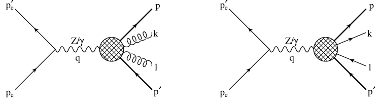
Figure 3.1: Four-body kinematics.

The four-body processes we are considering are illustrated in Fig. 3.1, and summarized by

$$e^{+}\left(p_{e}^{\prime}\right)+e^{-}\left(p_{e}\right)\ \,\mbox{$\rightarrow$}\ \,Z/\gamma\,(q)\!\! \rightarrow \!\!Q(p)+\overline{Q}(p^{\prime})+g(k)+g(l)$$

$$e^{+}\left(p_{e}^{\prime}\right)+e^{-}\left(p_{e}\right)\ \,\mbox{$\rightarrow$}\ \,Z/\gamma\,(q)\!\! \rightarrow \!\!Q(p)+\overline{Q}(p^{\prime})+q(k)+\bar{q}(l)\;,$$

where $Q$ is the massive quark, $q$ is the massless quark and the momenta satisfy

$$l^{2}=k^{2}=0\;,\quad\quad\quad p^{2}=p^{\prime 2}=m^{2}\;,\quad\quad\quad q^{2}=\left(p_{e}^{\prime}+p_{e}\right)^{2}\;.$$ (3.1)

We hope that no confusion arises between the total momentum $q$ and the light quark $q$. In the centre-of-mass system of the two massless particles, we can express the $d$-momenta in the following way

$$l = l_{0}\,\bigl{(}1,\ldots,\sin\theta\sin\phi,\sin\theta\cos\phi,\cos\theta\bigr{)}$$ (3.2)

$$k = k_{0}\,\bigl{(}1,\ldots,-\sin\theta\sin\phi,-\sin\theta\cos\phi,-\cos\theta\bigr{)}$$ (3.3)

$$p = p_{0}\left(1,\ldots,0,0,\sqrt{1-\frac{m^{2}}{p_{0}^{2}}}\right)$$ (3.4)

$$p^{\prime} = p^{\prime}_{0}\left(1,\ldots,0,\sqrt{1-\frac{m^{2}}{{p^{\prime}_{0}}^{2}}}\sin\alpha,\sqrt{1-\frac{m^{2}}{{p^{\prime}_{0}}^{2}}}\cos\alpha\right)\;,$$ (3.5)

where the dots indicate $d-3$ equal and opposite components in the expression for $l$ and $k$, and $d-3$ zeros in the expression for $p$ and $p^{\prime}$.

To describe the unoriented four-body phase space, we need five independent variables, which we choose to be

$$x_{1}=\frac{2q\cdot p}{q^{2}}\;,\quad\quad x_{2}=\frac{2q\cdot p^{\prime}}{q^{2}}\;,\quad\quad y=\frac{(k+l)^{2}}{q^{2}}\;,\quad\quad\theta,\quad\quad\phi\;.$$ (3.6)

In the centre-of-mass system of the light particles

$$l_{0}=k_{0}=\sqrt{q^{2}}\,\frac{\sqrt{y}}{2}\;,$$ (3.7)

where we have used the definition of $y$ of eq. (3.6). From momentum conservation, written in the following way,

  $${(q-p)^{2}=(p^{\prime}+k+l)^{2}} {(q-p^{\prime})^{2}=(p+k+l)^{2}\;,}$$   (3.8)

we have

$$p_{0}=\sqrt{q^{2}}\,\frac{1-x_{2}-y}{2\sqrt{y}}\;,\quad\quad\quad p^{\prime}_{0}=\sqrt{q^{2}}\,\frac{1-x_{1}-y}{2\sqrt{y}}\;,$$ (3.9)

and from

$$(p+p^{\prime}+k+l)^{2}=q^{2}\;,$$ (3.10)

we obtain

$$\left(p_{0}+p_{0}^{\prime}+\sqrt{q^{2}}\sqrt{y}\right)^{2}-\left(p_{0}^{\prime 2}-m^{2}\right)\sin^{2}\alpha-\left(\sqrt{p_{0}^{2}-m^{2}}+\sqrt{p_{0}^{\prime 2}-m^{2}}\cos\alpha\right)^{2}=q^{2}\;.$$

We can solve this expression to give

$$\cos\alpha=\frac{y\,(\rho-x_{1}-x_{2})+(1-x_{1})(1-x_{2})-y^{2}}{\sqrt{\left(1-x_{1}-y\right)^{2}-4\rho\,y}\;\sqrt{\left(1-x_{2}-y\right)^{2}-4\rho\,y}}\;,$$ (3.11)

where

$$\rho=\frac{4m^{2}}{q^{2}}\;.$$ (3.12)

Starting from the four-particle phase space in $d$ dimensions

$$d\Phi_{4}=\int\frac{d^{d-1}p}{2\,p_{0}(2\pi)^{d-1}}\,\frac{d^{d-1}p^{\prime}}{2\,p^{\prime}_{0}(2\pi)^{d-1}}\,\frac{d^{d-1}l}{2\,l_{0}(2\pi)^{d-1}}\,\frac{d^{d-1}k}{2\,k_{0}(2\pi)^{d-1}}\,(2\pi)^{d}\,\delta^{d}(q-p-p^{\prime}-l-k)\;,$$ (3.13)

we introduce the following two identities

$$\int\frac{d^{d}t}{(2\pi)^{d}}\,(2\pi)^{d}\,\delta^{d}(t-l-k)=1\;,\quad\quad\quad q^{2}\,\int\frac{dy}{2\pi}\,2\pi\,\delta(t^{2}-q^{2}\,y)=1\;,$$ (3.14)

which allow us to integrate eq. (3.13) in $t_{0}$, and to obtain

$$d\Phi_{4}\! = \!q^{2}\int\frac{dy}{2\pi}\,\Theta(y)\,\underbrace{\frac{d^{d-1}t}{2\,t_{0}(2\pi)^{d-1}}\,\frac{d^{d-1}p}{2\,p_{0}(2\pi)^{d-1}}\,\frac{d^{d-1}p^{\prime}}{2\,p^{\prime}_{0}(2\pi)^{d-1}}\,(2\pi)^{d}\,\delta^{d}(q-t-p-p^{\prime})}_{d\Phi_{3}}$$ (3.15)

$$\phantom{\int\frac{dy}{2\pi}\,\Theta(y)\,}\times\underbrace{\frac{d^{d-1}l}{2\,l_{0}(2\pi)^{d-1}}\,\frac{d^{d-1}k}{2\,k_{0}(2\pi)^{d-1}}\,(2\pi)^{d}\,\delta^{d}(t-k-l)}_{d\Phi_{2}}\;,$$

where

$$t_{0}=\sqrt{|{\bf t}|^{2}+q^{2}y}\;,$$ (3.16)

and where $\Theta(y)$ is the Heaviside function. In this way we succeed in dividing the four-body phase space into two simpler Lorentz-invariant scalars, that we can evaluate in the most appropriate reference system.

We compute $d\Phi_{2}$ in the centre-of-mass system of the two massless particles. In this system

$${\bf t}={\bf k}+{\bf l}={\bf 0}\;,\quad\quad\quad t_{0}=k_{0}+l_{0}=\sqrt{q^{2}}\sqrt{y}\;,$$ (3.17)

where we have used eq. (3.7). Integrating in $k$, we get

$$d\Phi_{2} = \int\frac{d^{d-1}l}{2\,l_{0}(2\pi)^{d-1}}\,\frac{1}{2\,k_{0}}\,2\pi\,\delta(t_{0}-k_{0}-l_{0})=\int\frac{d^{d-1}l}{4\,l_{0}^{2}\,(2\pi)^{d-2}}\,\delta(t_{0}-2\,l_{0})$$

$$= \int\frac{dl_{y}\,dl_{z}\,dl^{d-3}_{\perp}}{4\,l_{0}^{2}\,(2\pi)^{d-2}}\,\delta(t_{0}-2\,l_{0})=\int\frac{dl_{y}\,dl_{z}\,|{\bf l_{\perp}}|^{d-4}d|{\bf l_{\perp}}|\,d\Omega^{d-3}}{4\,l_{0}^{2}\,(2\pi)^{d-2}}\,\delta(t_{0}-2\,l_{0})\;,$$

where we have introduced the integration over the solid angle $\Omega$ in $d-3$ dimensions:

$$\Omega^{d}\equiv\int d\Omega^{d}=\frac{2\,\pi^{\frac{d}{2}}}{\Gamma\left(\frac{d}{2}\right)}\;.$$ (3.18)

We perform the following change of variables

$$l_{y} = l_{0}\sin\theta\cos\phi$$

$$l_{z} = l_{0}\cos\theta$$ (3.19)

$$|{\bf l_{\perp}}| = \sqrt{|{\bf l}|^{2}-l_{y}^{2}-l_{z}^{2}}=l_{0}\sin\theta\sin\phi\;,$$ (3.20)

with Jacobian

$$dl_{y}\,dl_{z}\,d|{\bf l_{\perp}}|=l_{0}^{2}\,\sin\theta\,d\theta\,d\phi\,dl_{0}\;,$$ (3.21)

and considering that $|{\bf l}|=l_{0}$, we can write

$$d\Phi_{2}=\int\frac{d\theta\,d\phi\,dl_{0}}{4\,l_{0}^{2}\,(2\pi)^{d-2}}\,l_{0}^{d-2}\,\sin\theta\,\left(\sin\theta\sin\phi\right)^{d-4}\,\frac{2\,\pi^{\frac{d-3}{2}}}{\Gamma\left(\frac{d-3}{2}\right)}\,\delta(t_{0}-2\,l_{0})\;.$$ (3.22)

The integration over $l_{0}$ is straightforward and, with the last change of variable

$$v=\frac{1}{2}(1-\cos\theta)\;,$$ (3.23)

we have, in $d=4-2\epsilon$ dimensions,

$$d\Phi_{2}=\frac{1}{8\pi}\,\frac{\left(4\pi\right)^{\epsilon}}{\Gamma(1-\epsilon)}\left(q^{2}y\right)^{-\epsilon}\int_{0}^{1}dv\,[v(1-v)]^{-\epsilon}\frac{1}{N_{\phi}}\int_{0}^{\pi}d\phi\,(\sin\phi)^{-2\epsilon}\;,$$ (3.24)

where

$$N_{\phi}=\int_{0}^{\pi}d\phi\,(\sin\phi)^{-2\epsilon}=4^{\epsilon}\pi\frac{\Gamma(1-2\epsilon)}{\Gamma^{2}(1-\epsilon)}$$ (3.25)

and where we have used eq. (3.17).

We can immediately integrate in $t$ the three-body phase space of eq. (3.15) to obtain

$$d\Phi_{3}=\int\frac{2\pi}{2\,t_{0}}\,\frac{d^{d-1}p}{2\,p_{0}(2\pi)^{d-1}}\,\frac{d^{d-1}p^{\prime}}{2\,p^{\prime}_{0}(2\pi)^{d-1}}\,\delta(q_{0}-t_{0}-p_{0}-p_{0}^{\prime})$$ (3.26)

with the condition

$${\bf q}={\bf t}+{\bf p}+{\bf p^{\prime}}\;.$$ (3.27)

We evaluate this integral in the laboratory frame, where

$$q=(q_{0},{\bf 0})\;,\quad\quad\quad{\bf t}=-{\bf p}-{\bf p^{\prime}}\;.$$ (3.28)

We orient our reference axes in such a way that ${\bf p}$ is along the $z$ axis and ${\bf p^{\prime}}$ belongs to the $yz$ plane, forming an angle $\beta$ with ${\bf p}$. In this system

$$d^{d-1}p = |{\bf p}|^{d-2}\,d|{\bf p}|\,\Omega^{d-1}$$

$$d^{d-1}p^{\prime} = dp_{z}^{\prime}\,d^{d-2}p^{\prime}_{\perp}=dp^{\prime}_{z}\,|{\bf p^{\prime}_{\perp}}|^{d-3}d|{\bf p^{\prime}_{\perp}}|\,\Omega^{d-2}=|{\bf p^{\prime}}|\,d|{\bf p^{\prime}}|\,d\beta|{\bf p^{\prime}_{\perp}}|^{d-3}\,\Omega^{d-2}$$ (3.29)

$$= |{\bf p^{\prime}}|^{d-2}\,d|{\bf p^{\prime}}|\,\left(\sin\beta\right)^{d-3}\,d\beta\,\Omega^{d-2}\;,$$

where we have used

$$p^{\prime}_{z} = |{\bf p^{\prime}}|\cos\beta$$

$$|{\bf p^{\prime}_{\perp}}| = |{\bf p^{\prime}}|\sin\beta\;,$$

so that eq. (3.26) can be written

$$d\Phi_{3}=\int\frac{2\pi}{2\,t_{0}}\,\frac{|{\bf p}|^{d-2}\,d|{\bf p}|\,\Omega^{d-1}}{2\,p_{0}(2\pi)^{d-1}}\,\frac{|{\bf p^{\prime}}|^{d-2}\,d|{\bf p^{\prime}}|\,\Omega^{d-2}\left(\sin\beta\right)^{d-4}d\cos\beta}{2\,p^{\prime}_{0}(2\pi)^{d-1}}\,\delta(q_{0}-t_{0}-p_{0}-p_{0}^{\prime})\;.$$ (3.30)

From eqs. (3.16) and (3.28) we have

$$t_{0}=\sqrt{|{\bf p}|^{2}+|{\bf p}|^{2}+2\,|{\bf p}||{\bf p^{\prime}}|\cos\beta+q^{2}y}\;,\quad\quad\quad\quad\frac{\partial t_{0}}{\partial\cos\beta}=\frac{|{\bf p}||{\bf p^{\prime}}|}{t_{0}}\;,$$ (3.31)

and we can integrate in $\beta$ to obtain

$$d\Phi_{3}=\int\pi\,\frac{|{\bf p}|^{d-3}\,d|{\bf p}|\,\Omega^{d-1}}{2\,p_{0}(2\pi)^{d-1}}\,\frac{|{\bf p^{\prime}}|^{d-3}\,d|{\bf p^{\prime}}|\,\Omega^{d-2}\left(\sin\beta\right)^{d-4}}{2\,p^{\prime}_{0}(2\pi)^{d-1}}\;,$$ (3.32)

with $\beta$ determined by the $\delta$-function argument

$$q_{0}-p_{0}-p^{\prime}_{0}=\sqrt{|{\bf p}|^{2}+|{\bf p}|^{2}+2\,|{\bf p}||{\bf p^{\prime}}|\cos\beta+q^{2}y}\;.$$ (3.33)

If we evaluate $x_{1}$ and $x_{2}$ of eq. (3.6) in the laboratory system, we get

$$x_{1}=\frac{2\,p_{0}}{q_{0}}\;,\quad\quad\quad\quad x_{2}=\frac{2\,p^{\prime}_{0}}{q_{0}}\;,$$ (3.34)

and considering that

$$|{\bf p}|^{2}=p_{0}^{2}-m^{2}=\frac{q^{2}}{4}\left(x_{1}^{2}-\rho\right)\;,\quad\quad\quad|{\bf p^{\prime}}|^{2}=p_{0}^{\prime 2}-m^{2}=\frac{q^{2}}{4}\left(x_{2}^{2}-\rho\right)\;,$$ (3.35)

we can write $d\Phi_{3}$ as

$$d\Phi_{3} = \frac{1}{\Gamma(2-2\epsilon)}\,\frac{(8\pi)^{2\epsilon}}{2\,(4\pi)^{3}}\,(q^{2})^{1-2\epsilon}\!\!\int dx_{1}\,dx_{2}\,\left(\sin\beta\right)^{-2\epsilon}\left(x_{1}^{2}-\rho\right)^{-\epsilon}\left(x_{2}^{2}-\rho\right)^{-\epsilon}$$

$$= \frac{1}{\Gamma(2-2\epsilon)}\,\frac{(8\pi)^{2\epsilon}}{2\,(4\pi)^{3}}\,(q^{2})^{1-2\epsilon}\!\!\int dx_{1}\,dx_{2}\,\left(1-\cos^{2}\beta\right)^{-\epsilon}\left(x_{1}^{2}-\rho\right)^{-\epsilon}\left(x_{2}^{2}-\rho\right)^{-\epsilon}\;.$$

From eq. (3.33), we have

$$\cos\beta=\frac{\left(x_{g}^{2}-4\,y\right)-\left(x_{1}^{2}-\rho\right)-\left(x_{2}^{2}-\rho\right)}{2\sqrt{x_{1}^{2}-\rho}\sqrt{x_{2}^{2}-\rho}}\;,$$ (3.37)

where we define

$$x_{g}\equiv 2-x_{1}-x_{2}\;,$$ (3.38)

and the integration range for $x_{1}$ and $x_{2}$ is determined by the reality condition for $\cos\beta$

$$-1\leq\cos\beta\leq 1\;.$$ (3.39)

Inserting the expressions of eqs. (3.24) and (3.1) into eq. (3.15), we obtain

$$d\Phi_{4} = \frac{q^{2}}{(4\pi)^{2}\,\Gamma(1-\epsilon)}\left(\frac{4\pi}{q^{2}}\right)^{\epsilon}H\int dx_{1}\,dx_{2}\,dy\,y^{-\epsilon}\,\Theta(y)$$ (3.40)

$$\times\left\{4\left(x_{1}^{2}-\rho\right)\left(x_{2}^{2}-\rho\right)-\left[(x_{g}^{2}-4\,y)-(x_{1}^{2}-\rho)-(x_{2}^{2}-\rho)\right]^{2}\right\}^{-\epsilon}$$

$$\times\int_{0}^{1}dv\,[v(1-v)]^{-\epsilon}\,\frac{1}{N_{\phi}}\int_{0}^{\pi}d\phi\,(\sin\phi)^{-2\epsilon}\;,$$

with

$$H\equiv\frac{1}{\Gamma(2-2\epsilon)}\,\frac{q^{2}}{2\,(4\pi)^{3}}\,\left(\frac{16\pi}{q^{2}}\right)^{2\epsilon}\;.$$ (3.41)

The last step to perform is the determination of the integration region. First of all, the physical boundaries for the integration variables are

$$\sqrt{\rho}\leq x_{1},x_{2}\leq 1\;,\quad\quad\quad 0\leq y\leq\left(1-\sqrt{\rho}\right)^{2}\;.$$ (3.42)

If we choose to integrate first in $y$, we solve eq. (3.39) with respect to $y$, and we get

$$y_{-}\leq y\leq y_{+}\;,$$ (3.43)

with

$$y_{\pm}\equiv\frac{1}{4}\left[x_{g}^{2}-(x_{1}^{2}-\rho)-(x_{2}^{2}-\rho)\pm 2\sqrt{x_{1}^{2}-\rho}\sqrt{x_{2}^{2}-\rho}\right]\;.$$ (3.44)

The Heaviside function $\Theta(y)$ of eq. (3.40) imposes the condition

$$y_{+}\geq 0\;,$$ (3.45)

which forces the allowed regions for $x_{1}$ and $x_{2}$ integration to be “region I” and “region II” of Fig. 3.2.

Figure 3.2: The two different areas in the $x_{1}$-$x_{2}$ plane correspond to the region I and to the region II of eq. (3.52).

In these regions, the relation

$$y\leq\left(1-\sqrt{\rho}\right)^{2}$$ (3.46)

is always satisfied. In addition, we have

$$y_{-}\geq 0{\rm\ \ \ if\ \ \ }x_{1},x_{2}\in{\rm region\ II}\;.$$ (3.47)

Following this procedure, we succeed in dividing the phase space into two regions:

1. region I: $y$ can reach zero, where collinear and soft divergences arise. The integration range is (see Fig. 3.2)

   $$\int_{\sqrt{\rho}}^{1}dx_{1}\int_{x_{2-}}^{x_{2+}}dx_{2}\int_{0}^{y_{+}}dy\;,$$ (3.48)

   where

   $$x_{2\pm}=\frac{1}{4(1-x_{1})+\rho}\left[2\left(1-x_{1}\right)\left(2-x_{1}\right)+\rho\left(2-x_{1}\right)\pm 2\left(1-x_{1}\right)\sqrt{x_{1}^{2}-\rho}\right]$$ (3.49)

2. region II: $y$ cannot reach $0$ and the region is free from infrared divergences. The integration range is

   $$\int_{\sqrt{\rho}}^{x_{1+}}dx_{1}\int_{\sqrt{\rho}}^{x_{2-}}dx_{2}\int_{y_{-}}^{y_{+}}dy\;,$$ (3.50)

   where

   $$x_{1+}=2-\frac{2-\rho}{2-\sqrt{\rho}}\;.$$ (3.51)

We can then summarize the full four-body phase space

$$d\Phi_{4} = \frac{q^{2}}{(4\pi)^{2}\,\Gamma(1-\epsilon)}\left(\frac{4\pi}{q^{2}}\right)^{\epsilon}H$$ (3.52)

$$\times\Biggl{\{}\underbrace{\int_{\sqrt{\rho}}^{1}dx_{1}\int_{x_{2-}}^{x_{2+}}dx_{2}\int_{0}^{y_{+}}dy}_{\rm{region\ I}}\,+\underbrace{\int_{\sqrt{\rho}}^{x_{1+}}dx_{1}\int_{\sqrt{\rho}}^{x_{2-}}dx_{2}\int_{y_{-}}^{y_{+}}dy}_{\rm{region\ II}}\Biggr{\}}\,y^{-\epsilon}$$

$$\times\left\{4\left(x_{1}^{2}-\rho\right)\left(x_{2}^{2}-\rho\right)-\left[(x_{g}^{2}-4y)-(x_{1}^{2}-\rho)-(x_{2}^{2}-\rho)\right]^{2}\right\}^{-\epsilon}$$

$$\times\int_{0}^{1}dv\,[v(1-v)]^{-\epsilon}\,\frac{1}{N_{\phi}}\int_{0}^{\pi}d\phi\,(\sin\phi)^{-2\epsilon}\;.$$

A statistical factor $1/2!$ must be supplied if we consider the final state with the two identical gluons.

Sometimes we will need an analogous set of final-state variables, in which the role of $p$ and $p^{\prime}$ is interchanged. The variable $y$ remains the same, $x_{1}$ and $x_{2}$ are exchanged, and the other two variables, denoted by $v^{\prime}$ and $\phi^{\prime}$, are related to $v$ and $\phi$ by the equations

  $${v^{\prime}=\frac{1}{2}\left(1-\cos\theta^{\prime}\right)=\frac{1}{2}\left[1-\cos\alpha-\left(2\,\sqrt{v\,(1-v)}\cos\phi\sin\alpha-2\,v\cos\alpha\right)\right]} {\cos\phi^{\prime}=\frac{1-\cos\alpha-2\,(v-v^{\prime}\cos\alpha)}{2\sin\alpha\,\sqrt{v^{\prime}(1-v^{\prime})}}\;.}$$   (3.53)

These relations can be obtained considering the definition of the involved angles

  $${{\bf p^{\prime}}\cdot{\bf k}=|{\bf p^{\prime}}||{\bf k}|\left(\sin\theta\cos\phi\sin\alpha+\cos\theta\cos\alpha\right)\equiv|{\bf p^{\prime}}||{\bf k}|\cos\theta^{\prime}} {{\bf p}\cdot{\bf k}=|{\bf p}||{\bf k}|\cos\theta\equiv|{\bf p}||{\bf k}|\left(\sin\alpha\sin\theta^{\prime}\cos\phi^{\prime}+\cos\theta^{\prime}\cos\alpha\right)\;,}$$   (3.54)

where the same scalar products have been computed in the reference system of eqs. (3.2)–(3.5) and in the reference system where $p$ and $p^{\prime}$ have been interchanged.

Exchanging the roles of $l$ and $k$ brings about the following transformations

$$v\,\mbox{$\rightarrow$}\,1-v\;,\quad\quad\quad\phi\,\mbox{$\rightarrow$}\,\pi+\phi\;,\quad\quad\quad v^{\prime}\,\mbox{$\rightarrow$}\,1-v^{\prime}\;,\quad\quad\quad\phi^{\prime}\,\mbox{$\rightarrow$}\,\pi+\phi^{\prime}\;.$$ (3.55)

3.2 Kinematics and three-body phase space with one massless particle

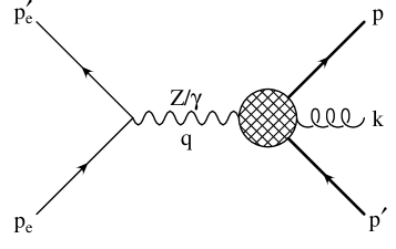
Figure 3.3: Three-body kinematics.

We consider the three-body process depicted in Fig. 3.3

$$e^{+}\left(p_{e}^{\prime}\right)+e^{-}\left(p_{e}\right)\;\mbox{$\rightarrow$}\;Z/\gamma\,(q)\;\mbox{$\rightarrow$}\;Q(p)+\overline{Q}(p^{\prime})+g(k)\;,$$ (3.56)

where the momenta of the particles satisfy

$$p^{2}=p^{\prime 2}=m^{2}\;,\quad\quad\quad k^{2}=0\;.$$ (3.57)

For unoriented shape variables, we can express the three-body phase space in terms of two variables, that we choose to be $x_{1}$ and $x_{2}$ of eq. (3.6). Using eqs. (3.1) and (3.37) we have

$$d\Phi_{3} = H\int_{\sqrt{\rho}}^{1}dx_{1}\int_{x_{2-}}^{x_{2+}}dx_{2}$$ (3.58)

$$\times\left\{4\left(x_{1}^{2}-\rho\right)\left(x_{2}^{2}-\rho\right)-\left[x_{g}^{2}-(x_{1}^{2}-\rho)-(x_{2}^{2}-\rho)\right]^{2}\right\}^{-\epsilon}\;,$$

where we put $y=0$, because the mass of the light system is zero (final gluon on-shell). The integration range can be found by imposing the reality condition (3.39), with $y=0$.

3.3 Kinematics and four-body phase space with four massive
particles

Figure 3.4: Four massive body kinematics.

The four-body process describing the production of four massive quarks is illustrated in Fig. 3.4 and summarized by

$$e^{+}\left(p_{e}^{\prime}\right)+e^{-}\left(p_{e}\right)\;\mbox{$\rightarrow$}\;Z/\gamma\,(q)\;\mbox{$\rightarrow$}\;Q(p)+\overline{Q}(p^{\prime})+Q(r)+\overline{Q}(r^{\prime})\;,$$ (3.59)

where

$$r^{2}=r^{\prime 2}=p^{2}=p^{\prime 2}=m^{2}\;.$$

The four-body phase space is obtained with a procedure similar to the one given in Sec. 3.1, with the simplification that now the entire cross section has no soft or collinear divergences, so that we can put ourselves directly in $d=4$ dimensions and we do not need to divide the allowed phase-space into two different regions. In the centre-of-mass frame of one heavy quark-antiquark pair we have

$$r = (r_{0},|{\bf r}|\sin\theta\sin\phi,|{\bf r}|\sin\theta\cos\phi,|{\bf r}|\cos\theta)$$

$$r^{\prime} = (r_{0},-|{\bf r}|\sin\theta\sin\phi,-|{\bf r}|\sin\theta\cos\phi,-|{\bf r}|\cos\theta)$$

$$p = p_{0}\left(1,0,0,\sqrt{1-\frac{m^{2}}{p_{0}^{2}}}\right)$$

$$p^{\prime} = p^{\prime}_{0}\left(1,0,\sqrt{1-\frac{m^{2}}{{p^{\prime}_{0}}^{2}}}\sin\alpha,\sqrt{1-\frac{m^{2}}{{p^{\prime}_{0}}^{2}}}\cos\alpha\right)\;,$$ (3.60)

where

$$y=\frac{(r+r^{\prime})^{2}}{q^{2}}\;\Longrightarrow\;r_{0}=\sqrt{q^{2}}\,\frac{\sqrt{y}}{2}\;,$$

and $p_{0}$, $p^{\prime}_{0}$ and $\cos\alpha$ are given by (3.9) and (3.11), while

$$|{\bf r}|=\sqrt{r_{0}^{2}-m^{2}}\;.$$ (3.61)

Starting from eq. (3.15), we need to re-compute the two-body phase space in $d=4$ dimensions for massive particles

$$d\Phi_{2}\!\! = \!\!\int\frac{d^{3}r}{2\,r_{0}(2\pi)^{3}}\,\frac{d^{3}r^{\prime}}{2\,r_{0}^{\prime}(2\pi)^{3}}\,(2\pi)^{4}\,\delta^{4}(t-r-r^{\prime})=\int\frac{d^{3}r}{4\,r_{0}^{2}\,(2\pi)^{2}}\,\delta\left(t_{0}-2r_{0}\right)$$ (3.62)

$$= \!\!\int\frac{|{\bf r}|^{2}d|{\bf r}|\,\sin\theta\,d\theta\,d\phi}{4\,r_{0}^{2}\,(2\pi)^{2}}\,\delta\left(t_{0}-2r_{0}\right)=\frac{1}{4}\frac{1}{(2\pi)^{2}}\sqrt{1-\frac{\rho}{y}}\int_{0}^{1}dv\int_{0}^{2\pi}d\phi\;,\phantom{aaaaaa}$$

where we have used eqs. (3.61) and (3.23). The four-body phase space, according to eqs. (3.15), (3.1) and (3.62) becomes

$$d\Phi_{4}=\frac{q^{4}}{\left(4\pi\right)^{6}}\int dy\,dx_{1}\,dx_{2}\sqrt{1-\frac{\rho}{y}}\int_{0}^{1}dv\int_{0}^{2\pi}d\phi\;.$$ (3.63)

The physical boundaries for the kinematical variables are

$$\rho\leq y\leq\left(1-\sqrt{\rho}\right)^{2}\;,\quad\quad\quad\sqrt{\rho}\leq x_{1},x_{2}\leq 1-2\rho\;,$$ (3.64)

and from the reality condition (3.39), we have

$$\bar{x}_{2-}\leq x_{2}\leq\bar{x}_{2+}\;,$$ (3.65)

where

$$\bar{x}_{2\pm}=\frac{1}{4(1-x_{1})+\rho}\left[(2-x_{1})(2+\rho-2y-2x_{1})\pm 2\sqrt{\left(x_{1}^{2}-\rho\right)\left[(x_{1}-1+y)^{2}-\rho\,y\right]}\right]$$ (3.66)

According to eq. (3.64), $\bar{x}_{2+}$ must satisfy

$$\bar{x}_{2+}\geq\sqrt{\rho}\;,$$ (3.67)

which implies

$$x_{1}\leq 1-y-\sqrt{\rho\,y}\;,$$ (3.68)

so we have

$$d\Phi_{4}=\frac{q^{4}}{\left(4\pi\right)^{6}}\int_{\rho}^{\bar{y}_{+}}dy\sqrt{1-\frac{\rho}{y}}\int_{\sqrt{\rho}}^{\bar{x}_{1+}}dx_{1}\int_{\bar{x}_{2-}}^{\bar{x}_{2+}}dx_{2}\int_{0}^{1}dv\int_{0}^{2\pi}d\phi\;,$$ (3.69)

where

  $${\bar{y}_{+}=\left(1-\sqrt{\rho}\right)^{2}} {\bar{x}_{1+}\!\!=1-y-\sqrt{\rho\,y}\;.}$$   (3.70)

A statistical factor $1/(2!2!)=1/4$ must be supplied to eq. (3.69), because of the presence of two pairs of identical particles in the final state.

Chapter 4 Next-to-leading-order amplitudes

4.1 Introduction and notation

In writing the amplitude for the process we are investigating, we disregard, at present, the contributions coming from the decay of the $Z/\gamma$ boson into a light couple of quarks. We postpone all the comments on this subject to Secs. 4.5 and 4.6.2. We can then write the amplitude, up to an irrelevant phase, as

$${\cal A} = \bar{v}(p_{e}^{\prime})\Bigg{[}g_{\rm\scriptscriptstyle Z}^{2}\,\frac{-g_{\mu\nu}}{q^{2}-M_{\rm{\rm\scriptscriptstyle Z}}^{2}+i\Gamma_{\rm{\rm\scriptscriptstyle Z}}M_{\rm{\rm\scriptscriptstyle Z}}}\left(v_{e}\gamma^{\mu}-a_{e}\gamma^{\mu}\gamma^{5}\right)\langle 0|J^{\nu}_{V}(0)v_{\rm\scriptscriptstyle Q}-J^{\nu}_{A}(0)a_{\rm\scriptscriptstyle Q}|f\rangle$$ (4.1)

$$\mbox{}+g^{2}\frac{-g_{\mu\nu}}{q^{2}}(c_{e}\gamma^{\mu})\langle 0|J^{\nu}_{V}(0)c_{\rm\scriptscriptstyle Q}|f\rangle\Bigg{]}u(p_{e})\;,$$

where $|f\rangle$ refers to states with four-momentum $q$ and $J_{V}(0)$, $J_{A}(0)$ are the currents that describe the decay of the vector boson into the final state $|f\rangle$. In this equation we see the contributions coming from the $\gamma$ propagator, second term, and the $Z$ propagator, first term, where we have neglected terms proportional to $q_{\mu}q_{\nu}$ because of leptonic current conservation, always verified for the vectorial part but verified in the massless limit for the axial part

$$\bar{v}(p_{e}^{\prime})\,q_{\mu}\,\Gamma_{V/A}^{\mu}\,u(p_{e})=0\quad\quad{\rm with}\quad\quad\Gamma_{V}^{\mu}=\gamma^{\mu}\;,\ \ \Gamma_{A}^{\mu}=\gamma^{\mu}\gamma^{5}{\rm\ \ and\ \ }m_{e}=0\;.$$ (4.2)

The notation used in eq. (4.1) is

$$g_{\rm{\rm\scriptscriptstyle Z}} \equiv \frac{g}{2\sin\theta_{\rm W}\cos\theta_{\rm W}}$$

$$v_{i} \equiv T_{3i}-2c_{i}\sin^{2}\theta_{\rm W}$$ (4.3)

$$a_{i} \equiv T_{3i}$$

where $g$ is the electromagnetic coupling, $T_{3i}$ is the third component of the (left) isospin of fermion $i$, $c_{i}$ is its electric charge in units of the positron charge and $\theta_{\rm W}$ is the Weinberg angle. $M_{\rm{\rm\scriptscriptstyle Z}}$ and $\Gamma_{\rm{\rm\scriptscriptstyle Z}}$ are the $Z$ mass and total decay width.

We are interested in describing only unoriented events: for this reason, we can neglect the axial-vector interference term in the square of the amplitude. In fact, for the three-parton final state of Fig. 3.3, there are not enough momenta to construct an invariant with an $\epsilon$ symbol. For the four-parton final state of Fig. 3.1, one could in principle build such an invariant, but the cross section must be symmetric in the light parton momenta, so that such an invariant cannot survive. This is strictly true for the $Q\overline{Q}gg$ final state, and for the state $Q\overline{Q}q\overline{q}$, if the weak current is coupled to the heavy quark. We refer to Sec. 4.6.2 for further details.

In addition, we have no problems between the use of the dimensional regularization procedure and the axial coupling. In fact, we can circumvent the presence of $\gamma_{5}$ considering the case of a generic vector current coupled to two fermions with different masses $m_{1}$ and $m_{2}$. One can easily convince oneself that the case of the axial coupling can be obtained by setting $m_{1}=m$ and $m_{2}=-m$, since one can turn $-m$ into $m$ by a chiral rotation. This procedure is bound to work if there are no anomalies involved in the calculation, and this is certainly the case for the graphs we have chosen to compute (see Secs. 4.4–4.6).

When squaring the amplitude to compute the differential cross section, we have two different tensorial structures which describe the leptonic and hadronic part of the process. The leptonic tensor, obtained by averaging over the initial polarization, is given by

$$L^{\mu\nu}=\frac{1}{4}\mathop{\rm Tr}\left(p\kern-4.30554pt\hbox{/}_{e}^{\prime}\,\Gamma^{\mu}_{V/A}\,p\kern-4.30554pt\hbox{/}_{e}\,\Gamma^{\nu}_{V/A}\right)=p_{e}^{\mu}\,{p^{\prime}}_{e}^{\nu}+p_{e}^{\nu}\,{p^{\prime}}_{e}^{\mu}-\left(p_{e}\!\cdot p^{\prime}_{e}\right)\,g^{\mu\nu}\;,$$ (4.4)

and, if we further average over the incoming electron beam direction, we obtain

$$\overline{L^{\mu\nu}}=\frac{q^{2}}{3}\left(-g^{\mu\nu}+\frac{q^{\mu}q^{\nu}}{q^{2}}\right)\;.$$ (4.5)

We can then write the differential cross section as

$$d\sigma = \frac{4\,\pi}{3\,q^{2}}\,\alpha^{2}N_{c}\bigg{\{}dT_{V}\left[\rho_{2}(q^{2})\,(v_{e}^{2}+a_{e}^{2})\,v_{\rm\scriptscriptstyle Q}^{2}+c_{e}^{2}\,c_{\rm\scriptscriptstyle Q}^{2}-2\,\rho_{1}(q^{2})\,v_{e}\,v_{\rm\scriptscriptstyle Q}\,c_{e}\,c_{\rm\scriptscriptstyle Q}\right]$$

$${}+dT_{A}\left[\rho_{2}(q^{2})\,(v_{e}^{2}+a_{e}^{2})\,a_{\rm\scriptscriptstyle Q}^{2}\right]\bigg{\}}\;,$$

where $\alpha=g^{2}/(4\pi)$ is the electromagnetic coupling constant, $N_{c}=3$ is the number of colours and

$$\rho_{1}(q^{2}) = \frac{1}{4\sin^{2}\theta_{\rm W}\cos^{2}\theta_{\rm W}}\;\frac{q^{2}\,(M_{\rm\scriptscriptstyle Z}^{2}-q^{2})}{(M_{\rm\scriptscriptstyle Z}^{2}-q^{2})^{2}+M_{\rm\scriptscriptstyle Z}^{2}\,\Gamma_{\rm\scriptscriptstyle Z}^{2}}$$

$$\rho_{2}(q^{2}) = \left(\frac{1}{4\sin^{2}\theta_{\rm W}\cos^{2}\theta_{\rm W}}\right)^{2}\frac{q^{4}}{(M_{\rm\scriptscriptstyle Z}^{2}-q^{2})^{2}+M_{\rm\scriptscriptstyle Z}^{2}\,\Gamma_{\rm\scriptscriptstyle Z}^{2}}\;.$$

We have also defined

$$dT_{V/A} = \sum_{n}{\cal M}^{(f_{n})}_{V/A}d\Phi_{n}$$

$${\cal M}^{(f_{n})}_{V/A} = \frac{2\pi}{N_{c}\,q^{2}}\left(-g_{\mu\nu}+\frac{q_{\mu}q_{\nu}}{q^{2}}\right)\langle 0|J^{\mu}_{V/A}(0)|f_{n}\rangle\langle f_{n}|J^{\nu}_{V/A}(0)|0\rangle\;,$$ (4.6)

where $d\Phi_{n}$ represents the $n$-body phase space, and $|f_{n}\rangle$ represents an $n$-body final state. The $q^{\mu}q^{\nu}$ term in the projector in eq. (4.6) is, of course, irrelevant for the vector current component, but it should be kept for the axial current when the quark mass is non-zero.

In the following we will be interested in strong corrections up to the second order, and in the final states: $Q\overline{Q}$, $Q\overline{Q}g$, $Q\overline{Q}gg$, $Q\overline{Q}q\bar{q}$ and $Q\overline{Q}Q\overline{Q}$. We will use the following simplified notation:

• ${\cal M}^{(2)}_{V/A}$ for the $Q\overline{Q}$ tree-level term

• ${\cal M}^{(b)}_{V/A}$ or ${\cal M}_{b}$ to indicate the three-body Born $Q\overline{Q}g$, ${\cal O}\left(\alpha_{s}\right)$ term

• ${\cal M}^{(v)}_{V/A}$ or ${\cal M}_{v}$ to indicate the three-body virtual $Q\overline{Q}g$, ${\cal O}\left(\alpha_{s}^{2}\right)$ term

• ${\cal M}^{(gg)}_{V/A}$ or ${\cal M}_{gg}$ for the four-body $Q\overline{Q}gg$, ${\cal O}\left(\alpha_{s}^{2}\right)$ term

• ${\cal M}^{(q\overline{q})}_{V/A}$ or ${\cal M}_{q\overline{q}}$ for the four-body $Q\overline{Q}q\overline{q}$, ${\cal O}\left(\alpha_{s}^{2}\right)$ term,

and equivalent ones for the $dT_{V/A}$ terms.

We will drop the ${V/A}$ suffix when not referring specifically to the axial or vector contribution.

4.2 $Q\overline{Q}$ cross section

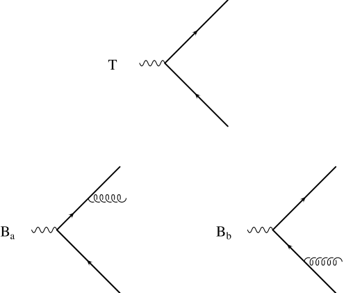
Figure 4.1: Tree (T) and Born (B) Feynman diagrams.

In the higher part of Fig. 4.1 we have depicted the Feynman diagram representing the tree-level amplitude

$${\cal A}^{\mu}_{V/A}=\overline{u}(p)\Gamma^{\mu}_{V/A}v(p^{\prime})\;,$$ (4.7)

that, once squared, gives, for the two-body contribution to eq. (4.6), at zeroth order in $\alpha_{s}$,

$${\cal M}_{V}^{(2)}=\frac{2\pi}{N_{c}\,q^{2}}N_{c}\,4\,q^{2}\,\left(1+\frac{\rho}{2}\right)\;,\quad\quad\quad{\cal M}_{A}^{(2)}=\frac{2\pi}{N_{c}\,q^{2}}N_{c}\,4\,q^{2}\beta^{2}\;,$$ (4.8)

where $\rho$ is defined in eq. (3.12) and

$$\beta=\sqrt{1-\rho}\;.$$ (4.9)

Multiplying eq. (4.8) by the 2-body phase space $\beta/(8\pi)$, we get the zeroth-order contributions to the total cross section

$$T_{V}^{(2)}=\beta\,\left(1+\frac{\rho}{2}\right)\;,\quad\quad\quad T_{A}^{(2)}=\beta^{3}\;.$$ (4.10)

This justifies our choice for the normalization factor in eq. (4.6): in the massless limit, $T_{V}^{(2)}=T_{A}^{(2)}=1$.

4.3 $Q\overline{Q}g$ cross section at order $\alpha_{s}$

The amplitude for the Born term represented in the lower part of Fig. 4.1 is

$${\cal A}^{\mu\sigma}_{V/A}=\overline{u}(p)\Bigg{[}\left(-ig_{s}t^{a}_{ij}\gamma^{\sigma}\right)\frac{p\kern-4.30554pt\hbox{/}+k\kern-4.30554pt\hbox{/}+m}{(p+k)^{2}-m^{2}}\Gamma^{\mu}_{V/A}$$ (4.11)

$${}+\Gamma^{\mu}_{V/A}\frac{p\kern-4.30554pt\hbox{/}-q\kern-4.30554pt\hbox{/}+m}{(p-q)^{2}-m^{2}}\left(-ig_{s}t^{a}_{ij}\gamma^{\sigma}\right)\Bigg{]}v(p^{\prime})\;,\phantom{aaaaaaa}$$

where $t_{ij}^{a}$ are the generators of SU($N_{c}$) gauge symmetry, $i$ and $j$ refer to the colour indexes of quarks, while $a$ to the colour index of the external gluon. We remind here that

$$\sum_{a=1}^{N_{c}^{2}-1}\sum_{k=1}^{N_{c}}t^{a}_{ik}\,t^{a}_{kj}=C_{F}\,\delta_{ij}\quad\quad\quad i,j=1\ldots N_{c}\;,$$ (4.12)

where

$$C_{F}=\frac{N_{c}^{2}-1}{2N_{c}}=\frac{4}{3}\quad{\rm for}\quad N_{c}=3\;.$$ (4.13)

We define

$$M^{\sigma\sigma^{\prime}}_{V/A}\equiv\frac{1}{g_{s}^{2}\,C_{F}N_{c}}\left(-g_{\mu\nu}+\frac{q_{\mu}q_{\nu}}{q^{2}}\right)\sum{\cal A}^{\mu\sigma}_{V/A}{\cal A}^{*\nu\sigma^{\prime}}_{V/A}$$ (4.14)

where the sum refers to the spin and colour of the quarks and to the colour of the gluon in the final state. In the Feynman gauge, the sum over the polarization of the final gluon gives

$$\sum_{\rm pol}\epsilon^{\sigma}(k)\,\epsilon^{\sigma^{\prime}}(k)=-g^{\sigma\sigma^{\prime}}$$ (4.15)

so that we can define

$$M_{V/A}=-g_{\sigma\sigma^{\prime}}\,M_{V/A}^{\sigma\sigma^{\prime}}\;.$$ (4.16)

We need the expressions for $M_{V/A}$ in $d=4-2\epsilon$ dimensions. Computing the trace in eq. (4.14),

$$M_{V} = 8\frac{x_{1}^{2}+x_{2}^{2}}{(1-x_{1})(1-x_{2})}+\frac{16}{(1-x_{1})^{2}(1-x_{2})^{2}}\left(\frac{m^{2}}{q^{2}}\right)\Bigl{[}2\,x_{1}x_{2}(x_{1}+x_{2})$$ (4.17)

$${}-3\,(x_{1}^{2}+x_{2}^{2})-8\,(1-x_{1})(1-x_{2})+2\Bigr{]}-\frac{32}{(1-x_{1})^{2}(1-x_{2})^{2}}\left(\frac{m^{2}}{q^{2}}\right)^{2}x_{g}^{2}$$

$${}-\frac{16\epsilon}{(1-x_{1})(1-x_{2})}\Biggl{[}x_{1}^{2}+x_{2}^{2}+(1-x_{1})(1-x_{2})+x_{g}-1$$

$${}-\left(\frac{m^{2}}{q^{2}}\right)\frac{x_{g}^{2}}{(1-x_{1})(1-x_{2})}\Biggr{]}+\frac{8\epsilon^{2}}{(1-x_{1})(1-x_{2})}x_{g}^{2}\;,$$

and

$$M_{A} = 8\frac{x_{1}^{2}+x_{2}^{2}}{(1-x_{1})(1-x_{2})}+\frac{16}{(1-x_{1})^{2}(1-x_{2})^{2}}\left(\frac{m^{2}}{q^{2}}\right)\Bigl{[}-12(x_{1}+x_{2}-2x_{1}x_{2})$$ (4.18)

$${}-11x_{1}x_{2}(x_{1}+x_{2})+8(x_{1}^{2}+x_{2}^{2})+x_{1}^{3}(x_{2}-1)+x_{2}^{3}(x_{1}-1)$$

$${}+2x_{1}^{2}x_{2}^{2}+4\Bigr{]}(1-\epsilon)+\frac{64}{(1-x_{1})^{2}(1-x_{2})^{2}}\left(\frac{m^{2}}{q^{2}}\right)^{2}x_{g}^{2}\,(1-\epsilon)$$

$${}+\frac{8\epsilon^{2}}{(1-x_{1})(1-x_{2})}x_{g}^{2}\;,$$

where $x_{1},x_{2}$ and $x_{g}$ are defined by (3.6) and (3.38). According to eq. (4.6) we have

$${\cal M}^{(b)}_{V/A}=\frac{2\pi}{q^{2}}\;C_{F}\,g_{s}^{2}\mu^{2\epsilon}\,M_{V/A}\;,$$ (4.19)

where $\mu$ is the mass parameter of dimensional regularization, introduced in order to keep $g_{s}$ dimensionless.

For a future use, we introduce now a unit three-vector ${\bf j}$, belonging to the event plane (i.e. the plane defined by ${\bf p}$, ${\bf p^{\prime}}$ and ${\bf k}$) and perpendicular to ${\bf k}$. In the centre-of-mass system of the process, we can then write

$${\bf j}^{2}=1\;,\hskip 28.45274pt{\bf k}\cdot{\bf j}=0\;,\hskip 28.45274pt{\bf j}=a\,{\bf p}+b\,{\bf k}\;.$$ (4.20)

The generalization of these equations is easily obtained. From the fact that $j$ is a unit, purely space-like vector, we have

$$j^{2}=j_{0}^{2}-{\bf j}^{2}=-1\quad\Longrightarrow\quad j_{0}=0\;.$$ (4.21)

Since $q=\left(q_{0},{\bf 0}\right)$

$$\begin{array}[]{l}q\cdot j=q_{0}j_{0}-{\bf q}\cdot{\bf j}=0\\ k\cdot j=k_{0}j_{0}-{\bf k}\cdot{\bf j}=0\;,\\ \end{array}$$ (4.22)

and

$$j=a\,p+b\,k+c\,q\;.$$ (4.23)

We can then determine the coefficients $a,b$ and $c$ by imposing the validity of eqs. (4.22)

$$q\cdot j = 0\quad\Longrightarrow\quad a\,(p\cdot q)+b\,(k\cdot q)+c\,q^{2}=0$$

$$k\cdot j = 0\quad\Longrightarrow\quad a\,(p\cdot k)+c\,(q\cdot k)=0\;,$$ (4.24)

that, once solved, give

$$a=\frac{N}{p\cdot k}\;,\quad\quad\quad c=-\frac{N}{q\cdot k}\;,\quad\quad\quad b=N\,\frac{\displaystyle\frac{q^{2}}{q\cdot k}-\frac{p\cdot q}{p\cdot k}}{q\cdot k}\;,$$ (4.25)

with $N$ determined by the normalization condition (4.21). From the expression of $j$ we can compute

$$p\cdot j = -\frac{1}{2\,x_{g}}\sqrt{q^{2}}\Big{[}x_{2}^{2}\left(4x_{1}-\rho-4\right)+x_{1}^{2}\left(4x_{2}-\rho-4\right)-2x_{1}x_{2}(\rho+6)$$ (4.26)

$${}+4\left(\rho+2\right)\left(x_{1}+x_{2}\right)-4(\rho+1)\Big{]}^{\frac{1}{2}}\;.$$

We are now in a position to give a decomposition of the tensor $M^{\sigma\sigma^{\prime}}$ of eq. (4.14) (we disregard from now on the suffix $V/A$) according to the direction of $j$: in fact, the Lorentz indexes of this tensor take origin from the composition of the three independent vectors $q$, $p$ and $k$. Using eq. (4.23), we substitute $j$ instead of $p$ so that we can write $M^{\sigma\sigma^{\prime}}$ in a quite general form

$$M^{\sigma\sigma^{\prime}}=M^{\perp}g^{\sigma\sigma^{\prime}}_{\perp}+M^{j}j^{\sigma}j^{\sigma^{\prime}}+\mbox{terms involving $q$ or $k$}\;,$$ (4.27)

where (see eq. (D.25))

$$g_{\perp}^{\sigma\sigma^{\prime}}\equiv g^{\sigma\sigma^{\prime}}-\frac{\eta^{\sigma}k^{\sigma^{\prime}}+\eta^{\sigma^{\prime}}k^{\sigma}}{\eta\cdot k}\;,$$ (4.28)

with $\eta=(k_{0},-{\bf k})$, so that

$$\eta^{2}=0\;,\quad\quad\quad\eta\cdot j=0\;,\quad\quad\quad q_{\sigma}\,g_{\perp}^{\sigma\sigma^{\prime}}=0\;.$$ (4.29)

Contracting eq. (4.27) with $g_{\perp\sigma\sigma^{\prime}}$ and with $j_{\sigma}j_{\sigma^{\prime}}$, we obtain, in $d=4$ dimensions

$$M^{j}=M^{\sigma}_{\sigma}+2\,M^{\sigma\sigma^{\prime}}j_{\sigma}j_{\sigma^{\prime}}\;.$$ (4.30)

This expression can easily be computed, starting from the consideration of the previous paragraph about the dependence of $M^{\sigma\sigma^{\prime}}$ from $q$, $p$, $k$, and from eqs. (4.22) and (4.26)

$$M^{j}_{V/A} = \frac{2\,c_{\scriptscriptstyle V/A}}{(1-x_{1})^{2}(1-x_{2})^{2}}\Big{[}4x_{1}x_{2}(x_{1}+x_{2})-\rho(x_{1}+x_{2})^{2}-4(x_{1}^{2}+x_{2}^{2})$$ (4.31)

$${}-12x_{1}x_{2}+4(\rho+2)(x_{1}+x_{2})-4(\rho+1)\Big{]}\;,$$

where

$$c_{\scriptscriptstyle V}=\rho+2\;,\quad\quad\quad\quad c_{\scriptscriptstyle A}=-2(\rho-1)\;.$$ (4.32)

We also define, consistently with our previous notation

$${\cal M}^{(b)\sigma\sigma^{\prime}}_{V/A}=\frac{2\pi}{q^{2}}\;C_{F}\,g_{s}^{2}\mu^{2\epsilon}\,M^{\sigma\sigma^{\prime}}_{V/A}\;,\quad\quad\quad\quad{\cal M}^{(b)\perp/j}_{V/A}=\frac{2\pi}{q^{2}}\;C_{F}\,g_{s}^{2}\mu^{2\epsilon}\,M^{\perp/j}_{V/A}\;.$$ (4.33)

In the cases when the $V/A$ suffix needs not be specified, we will simply write ${\cal M}_{b}^{\sigma\sigma^{\prime}}$, ${\cal M}_{b}^{\perp}$ and ${\cal M}_{b}^{j}$.

4.4 Virtual contributions

Corrections to the three-jet decay rate to order $\alpha_{s}^{2}$ come from the interference of the one-loop graphs with the tree-level Born ones. In Fig. 4.2 we have depicted these contributions.

The algebra to compute these terms in $d=4-2\epsilon$ dimensions has been carried out in a straightforward way, using a MACSYMA program, which reduces the original Feynman graphs to a linear combination of scalar, one-loop integrals. The scalar integrals have been computed analytically and their values are listed in Appendix B.

Loop corrections to on-shell external lines (not illustrated in Fig. 4.2) require particular attention.

We start from the self-energy corrections to heavy-flavour external lines. As described in Appendix C.1, the effect of the fermion self-energy correction to an external line, including the mass counterterm, is equivalent to multiply the external propagator by the factor $Z_{Q}$ of eq. (C.13), so that we have a contribution to ${\cal M}_{v}$ equal to

$$z_{q}\times{\cal M}_{b}=-N_{\epsilon}C_{F}g_{s}^{2}\left(\frac{\mu^{2}}{m^{2}}\right)^{\epsilon}\left(\frac{3}{\epsilon}+4\right)\times{\cal M}_{b}\;.$$ (4.34)

We have to consider also the diagrams obtained with the mass counterterm insertion in internal fermion lines. In fact, according to eq. (C.11), we have to add a counterterm $m_{c}$ in order to keep $m$ as the pole mass, after radiative corrections. These diagrams are depicted in Fig. 4.3.

Similar considerations apply to the self-energy corrections to external gluon lines. As remarked in Appendix C.2, gluon, ghost and light-fermion self-energy corrections to external gluon lines vanish in dimensional regularization. Only the correction coming from a heavy-flavour loop needs be considered, and it gives a contribution at order $\alpha_{s}^{2}$ equal to (see eq. (C.22))

$$z_{g}\times{\cal M}_{b}=-N_{\epsilon}T_{F}g_{s}^{2}\left(\frac{\mu^{2}}{m^{2}}\right)^{\epsilon}\frac{4}{3\epsilon}\times{\cal M}_{b}\;.$$ (4.35)

After that, charge renormalization is all that is needed, since we are computing a physical cross section. Charge renormalization in the mixed scheme of Ref. [26] is described in Appendix C.3. From eq. (C.24) we can see that the last correction to our virtual term is equal to

$$z_{\alpha_{s}}\times{\cal M}_{b}=g_{s}^{2}N_{\epsilon}\left[\left(\frac{4}{3\epsilon}T_{F}\,n_{\rm lf}-\frac{11}{3\epsilon}C_{A}\right)+\left(\frac{\mu^{2}}{m^{2}}\right)^{\epsilon}\frac{4}{3\epsilon}T_{F}\right]\times{\cal M}_{b}\;.$$ (4.36)

We can now summarize the combined effect of external line corrections and renormalization to be included with ${\cal M}_{v}$

$$N_{\epsilon}g_{s}^{2}\left(\frac{\mu^{2}}{m^{2}}\right)^{\epsilon}\Bigg{\{}-2\,C_{F}\left(\frac{3}{\epsilon}+4\right)+\left(\frac{4}{3\epsilon}T_{F}\,n_{\rm lf}-\frac{11}{3\epsilon}C_{A}\right)\left(\frac{\mu^{2}}{m^{2}}\right)^{-\epsilon}\Bigg{\}}\times{\cal M}_{b}\;.$$ (4.37)

The factor of 2 in front of the fermion external line corrections is to account for the two fermion lines.

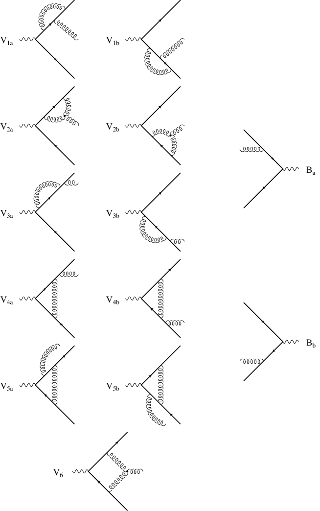
Figure 4.2: Radiative corrections to the process $Z/\gamma\,\mbox{$\rightarrow$}\,Q\overline{Q}g$. The interference of these diagrams (left hand side of the figure) with the tree-level Born term (right hand side) gives rise to contributions to order $\alpha_{s}^{2}$.

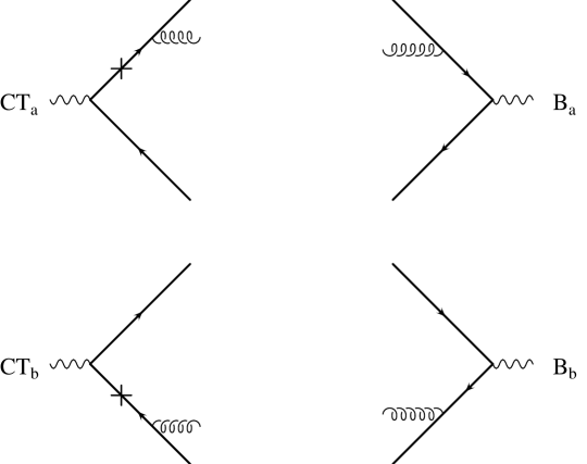
Figure 4.3: Contributions to order $\alpha_{s}^{2}$ coming from the interference between diagrams with the mass counterterm insertion and the tree-level Born term.

4.5 Hagiwara contributions

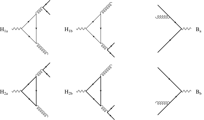
Figure 4.4: Radiative corrections to the process $Z/\gamma\,\mbox{$\rightarrow$}\,Q\overline{Q}g$ (Hagiwara contributions). The interference of these diagrams (left hand side of the figure) with the tree-level Born term (right hand side) gives rise to contributions to order $\alpha_{s}^{2}$.

At order $\alpha_{s}^{2}$, we have also contributions coming from the interference between terms in which the weak current is coupled to the heavy quarks and to quarks of different flavours.

These diagrams are represented in Fig. 4.4: the higher part of the figure describes the contributions coming from light-quark loops, while the lower part describes the contributions coming from heavy-quark loops.

By C-invariance (Furry’s theorem), these diagrams vanish for vector currents. For axial currents, they cancel in pairs of up-type and down-type quarks, because they have opposite axial coupling (see eqs. (4.3)), as long as the loop of different flavour may be regarded as massless. Thus, the up-quark contribution cancels with the down-quark, and, if the charm mass is neglected, the charm contribution cancels with the strange. Only the graph with a top quark loop remains.

Paired to this last type of diagrams are the contributions where the massive quark in the loop is the same as the heavy quark in the final state.

We have not included these diagrams in our calculation, because they have been computed in Ref. [14], where it was shown that their contribution is of order of $1\%$.

4.6 Real contributions

The square of the Feynman diagrams with four particles in the final state gives rise to the real contributions. These amplitudes are easily obtained, in an analytic form, with a little “Diracology” in $d=4$ dimensions. The behavior of these amplitudes in the soft and collinear limit is obtained in the next chapter, where the asymptotic forms of the amplitudes in derived in $d=4-2\epsilon$ dimensions.

4.6.1 Real contributions to the $Q\overline{Q}gg$ cross section

The diagrams contributing to the process

$$e^{+}e^{-}\,\mbox{$\rightarrow$}\,Z/\gamma\,\mbox{$\rightarrow$}\,Q\overline{Q}gg$$ (4.38)

are depicted in Fig. 4.5. From the square of these eight diagrams, we can obtain thirty-six terms, but most of them are related by interchange of the momentum labels, so that only thirteen amplitudes need be considered. We follow the notation used in Ref. [2], and indicate with Bij the interference of diagram Bi with diagram Bj (i$\geq$ j).

The different contributions to the cross section can be classified into three classes, according to their colour and spatial structure. We will always factorize out the colour factor common to the Born term, equal to $C_{F}\,N_{c}$, so that we have:

1. ${\mathbf{C}_{F}}$ class: planar QED-type diagrams

2. ${\mathbf{C}_{F}-\frac{1}{2}C_{A}}$ class: non-planar QED-type graphs

3. ${\mathbf{C}_{A}}$ class: QCD graphs, involving the three-gluon vertex

where $C_{A}=N_{c}$. In Tab. 4.1 we collect the thirty-six terms and the label interchanges, needed to compute all of them from the thirteen we have calculated (first row), and that are represented in Fig. 4.6. In the first row of this figure, there are the contributions belonging to the first class, in the second, the contributions to the second class and in the last row, the contributions to the third class.

permutation	${\mathbf{C}_{F}}$ class	${\mathbf{C}_{F}-\frac{1}{2}C_{A}}$ class	${\mathbf{C}_{A}}$ class
	B11 B21 B22 B32	B41 B42 B53 B52	B71 B72 B82 B77 B87
$(1\leftrightarrow 2)$	B11 B64 B66 B32	B41 B61 B53 B52	B84 B86 B76 B88 B87
$(3\leftrightarrow 4)$	B44 B54 B55 B65	B41 B51 B62 B52	B74 B75 B85 B77 B87
$(1\leftrightarrow 2)\,(3\leftrightarrow 4)$	B11 B31 B33 B32	B41 B43 B53 B63	B81 B83 B73 B77 B87

Table 4.1: Label interchanges needed to compute the thirty-six terms contributing to the process $e^{+}e^{-}\,\mbox{$\rightarrow$}\,Z/\gamma\,\mbox{$\rightarrow$}\,Q\overline{Q}gg$.

One final remark is needed, in order to sum over the final gluon polarizations. In fact, due to non-conservation of gluon current, we can use eq. (4.15) to sum over polarization only if we include B7- and B8-like diagrams with “external” ghost.

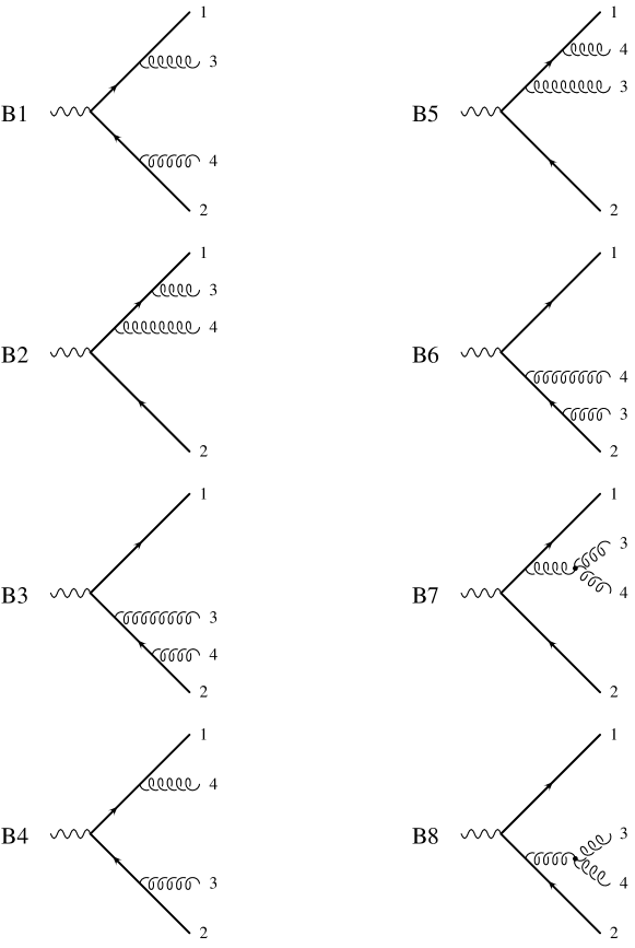
Figure 4.5: Feynman diagrams contributing to the process $Z/\gamma\,\mbox{$\rightarrow$}\,Q\overline{Q}gg$.

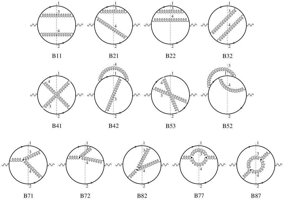
Figure 4.6: The thirteen amplitudes necessary to complete the computation of the cross section for the process $Z/\gamma\,\mbox{$\rightarrow$}\,Q\overline{Q}gg$. Cut propagators refer to on-shell particles, while numbers label the different momenta.

4.6.2 Real contributions to the $Q\overline{Q}q\overline{q}$ cross section

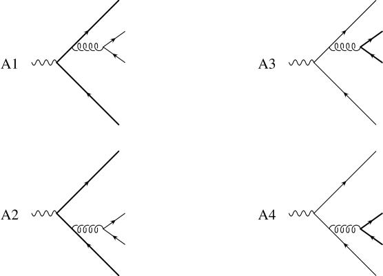
Figure 4.7: Feynman diagrams contributing to the process $Z/\gamma\,\mbox{$\rightarrow$}\,Q\overline{Q}q\overline{q}$.

The diagrams contributing to the process

$$e^{+}e^{-}\,\mbox{$\rightarrow$}\,Z/\gamma\,\mbox{$\rightarrow$}\,Q\overline{Q}q\overline{q}$$ (4.39)

are illustrated in Fig. 4.7.

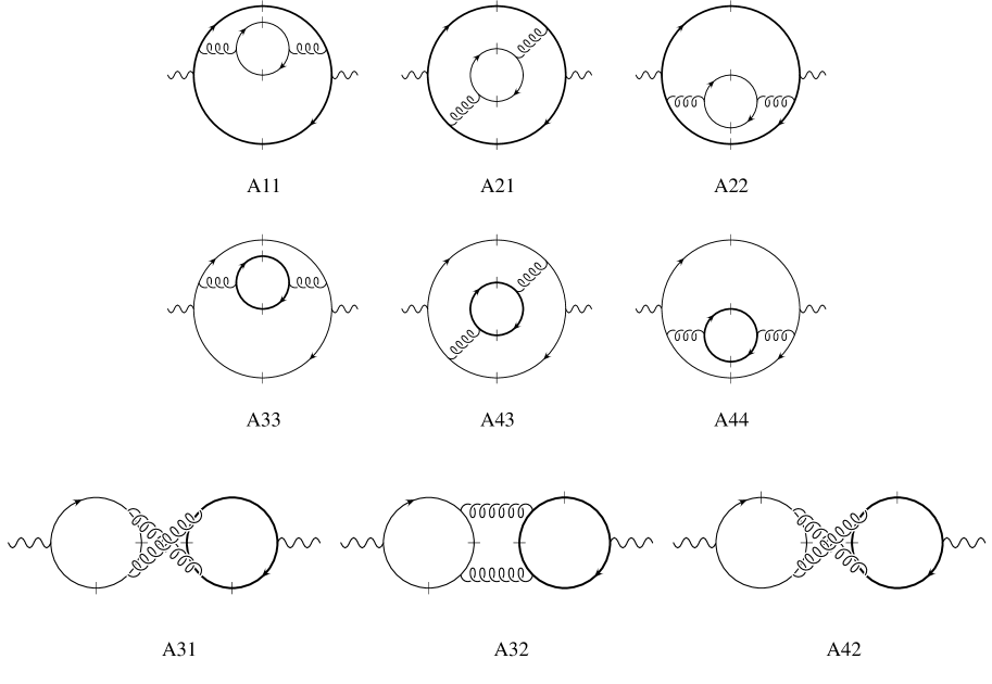
Figure 4.8: The nine amplitudes necessary to complete the computation of the cross section for the process $Z/\gamma\,\mbox{$\rightarrow$}\,Q\overline{Q}q\overline{q}$. Cut propagators refer to on-shell particles.

From the square of these four diagrams, we generate ten terms. In Fig. 4.8 we have depicted nine of them, because the tenth, A41, can be obtained with the massive loop of diagram A31 and the massless loop of diagram A42.

Although the colour coefficient is the same for all the ten diagrams (${\mathbf{T}_{F}}$), their infrared structure is different: in fact, only the diagrams in the first row of Fig. 4.8 contain infrared divergences, due to the massless-quark collinear region, all the other diagrams being finite.

For this reason, it is mandatory to include the first three diagrams, to check infrared cancellation, and it is custom to assign the other diagrams to the light channel: in fact, they are, in general, characterized by a large invariant mass for the light quarks and a small invariant mass for the heavy-quark couple. We have not included these last diagrams in our calculation.

4.6.3 Real contributions to the $Q\overline{Q}Q\overline{Q}$ cross section

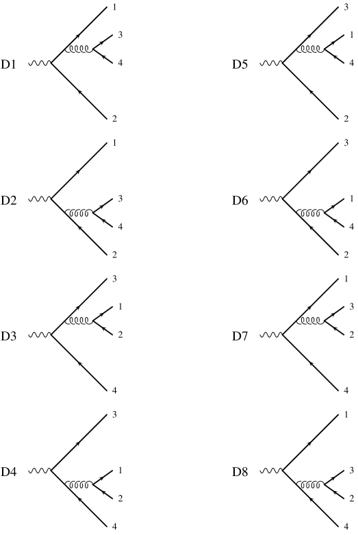
Figure 4.9: Feynman diagrams contributing to the process $Z/\gamma\,\mbox{$\rightarrow$}\,Q\overline{Q}Q\overline{Q}$.

The eight diagrams contributing to the process

$$e^{+}e^{-}\,\mbox{$\rightarrow$}\,Z/\gamma\,\mbox{$\rightarrow$}\,Q\overline{Q}Q\overline{Q}$$ (4.40)

are illustrated in Fig. 4.9.

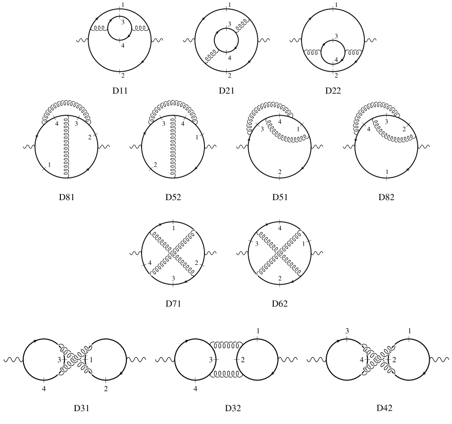
Figure 4.10: The twelve amplitudes necessary to complete the computation of the cross section for the process $Z/\gamma\,\mbox{$\rightarrow$}\,Q\overline{Q}Q\overline{Q}$. Cut propagators refer to on-shell particles, while numbers label the different momenta.

From the square of these diagrams we have thirty-six infrared-safe amplitudes. We need to compute only twelve of them, that we have represented in Fig. 4.10, because the others can be obtained by permuting the quark momenta. In Tab. 4.2 we give the twelve amplitudes we have computed (first row) and the label interchanges necessary to build all the others. As previously done for the $Q\overline{Q}gg$ process, we divide these contributions according to their colour factors and according to their structure:

1. ${\mathbf{1}^{\bf st}\ T_{F}}$ class: diagrams illustrated in the first row of Fig. 4.10

2. ${\mathbf{C}_{F}-\frac{1}{2}C_{A}}$ class: diagrams from D81 to D62

3. ${\mathbf{2}^{\bf nd}\ T_{F}}$ class: diagrams composed by two different massive loops, coupled to the weak current, that can be split apart by cutting the two joining gluon lines (singlet contributions).

permutation	${\mathbf{1}^{\bf st}\ T_{F}}$ class	${\mathbf{C}_{F}-\frac{1}{2}C_{A}}$ class	${\mathbf{2}^{\bf nd}\ T_{F}}$ class
	D11 D21 D22	D81 D52 D51 D82 D71 D62	D31 D32 D42
$(1\leftrightarrow 3)$	D55 D65 D66	D54 D61 D51 D64 D53 D62	D75 D76 D86
$(2\leftrightarrow 4)$	D77 D87 D88	D72 D83 D73 D82 D71 D84	D75 D85 D86
$(1\leftrightarrow 3)\,(2\leftrightarrow 4)$	D33 D43 D44	D63 D74 D73 D64 D53 D84	D31 D41 D42

Table 4.2: Label interchanges needed to compute the thirty-six terms contributing to the process $e^{+}e^{-}\,\mbox{$\rightarrow$}\,Z/\gamma\,\mbox{$\rightarrow$}\,Q\overline{Q}Q\overline{Q}$.

Chapter 5 Infrared cancellation

5.1 The subtraction method

In this section we want to introduce the method we have used in order to deal with the infrared divergences. In fact, as we have seen from the previous sections, infrared divergences arise both in the virtual and in the real terms:

1. in the virtual terms of Sec. 4.4, divergences arise from loop integration, as you can see from Appendix B. Since we have chosen to regularize our integrals with a dimensional method, we obtain poles in $\epsilon$;

2. in the real terms of Secs. 4.6.1 and 4.6.2, divergences in the differential cross section appear when we integrate over a particular region of the phase space. In the diagrams depicted in these sections, we have propagators proportional to $1/y$ (according to eq. (3.6), $y$ is proportional to the mass of the light system), so that we have divergences when integrating over the phase space region of small $y$. In this region, a four-particle final state masquerades as a three-particle event, because one of the emitted particles becomes soft, or two particles become collinear. Notice that the Born and the virtual graphs always have $y=0$.

According to Bloch-Nordsiek [27] and Kinoshita-Lee-Nauenberg [28] theorems, infrared divergences must cancel for sufficiently inclusive physical quantities.

Now, we show how we have checked this cancellation. If we compute the ${\cal O}\left(\alpha_{s}^{2}\right)$ differential cross section, in $d=4-2\epsilon$ dimensions, we get a result of the form

$$d\sigma=d\sigma^{(0)}+\left(\frac{\alpha_{s}}{2\pi}\right)d\sigma^{(1)}+\left(\frac{\alpha_{s}}{2\pi}\right)^{2}d\sigma^{(2)}\;,$$ (5.1)

with

$$d\sigma^{(2)}=\frac{d\sigma_{2}^{(2)}}{d\Phi_{2}}d\Phi_{2}+\frac{d\sigma_{3}^{(2)}}{d\Phi_{3}}d\Phi_{3}+\frac{d\sigma_{4}^{(2)}}{d\Phi_{4}}d\Phi_{4}\;,$$ (5.2)

where we sum up the contributions coming from two-, three- and four-particle final state. The two-particle final-state contribution at this order arises from the interference of two-loop diagrams with the tree-level term. We have not computed this differential cross section term, because we want to calculate only three-jet-related quantities, that give zero contribution in the two-jet limit. We give a detailed description of this fact in Sec. 5.2, so that we neglect $d\sigma_{2}^{(2)}$ in eq. (5.2).

Using eqs. (3.58) and (3.40), we can rewrite the three- and four-body phase space as

$$d\Phi_{3} = dx_{1}\,dx_{2}\,J_{3}(x_{1},x_{2})$$

$$d\Phi_{4} = dx_{1}\,dx_{2}\,dy\,d\theta\,d\phi\,J_{4}(x_{1},x_{2},y,\theta,\phi)\;,$$ (5.3)

where $J_{3}$ and $J_{4}$ represent all the other factors, whose exact structure we do not need to know in this section.

In order to implement the cancellation of the soft and collinear singularities, we now imagine to compute some physical quantity $G$ ($G$ stands for “Generic”), which depends on the final-state variables. $G$ may be a combination of theta functions that characterize a histogram bin for some infrared-safe shape variable, like the thrust, the $c$ parameter and the heavy-jet mass. In general the definition of $G$ is specified for any number of particles in the final state. Since we are dealing with three- and four-parton final states, $G$ is characterized by only two functions, $G_{3}(x_{1},x_{2})$ and $G_{4}(x_{1},x_{2},y,\theta,\phi)$. Soft and collinear finiteness of $G$ requires that

$$\lim_{y\mbox{$\rightarrow$}0}G_{4}(x_{1},x_{2},y,\theta,\phi)=G_{3}(x_{1},x_{2})\;.$$ (5.4)

When computing the contributions to $G$ at second order in $\alpha_{s}$, we have

$$\int d\sigma^{(2)}G = \int dx_{1}\,dx_{2}\,J_{3}(x_{1},x_{2})\frac{d\sigma_{3}^{(2)}}{d\Phi_{3}}\,G_{3}(x_{1},x_{2})$$ (5.5)

$${}+\int dx_{1}\,dx_{2}\,dy\,d\theta\,d\phi\,J_{4}(x_{1},x_{2},y,\theta,\phi)\,\frac{d\sigma_{4}^{(2)}}{d\Phi_{4}}\,G_{4}(x_{1},x_{2},y,\theta,\phi)\;,\phantom{aaaaa}$$

where each term on the right-hand side contains soft and collinear divergences that cancel in the sum. The integration of the complete differential cross section is too difficult to be performed analytically, but it is not a limiting point. In fact, we can add and subtract a suitable quantity, to obtain

  $${\int d\sigma^{(2)}G=\!\int\!dx_{1}dx_{2}\,G_{3}(x_{1},x_{2})\Bigg{\{}\frac{d\sigma_{3}^{(2)}}{d\Phi_{3}}J_{3}(x_{1},x_{2})+\!\int\!dy\,d\theta\,d\phi\frac{d\bar{\sigma}_{4}^{(2)}}{d\Phi_{4}}J_{4}(x_{1},x_{2},y,\theta,\phi)\!\Bigg{\}}} {\,\,\,+\int dx_{1}\,dx_{2}\,dy\,d\theta\,d\phi\,J_{4}(x_{1},x_{2},y,\theta,\phi)\Bigg{\{}\frac{d\sigma_{4}^{(2)}}{d\Phi_{4}}G_{4}(x_{1},x_{2},y,\theta,\phi)-\frac{d\bar{\sigma}_{4}^{(2)}}{d\Phi_{4}}G_{3}(x_{1},x_{2})\!\Bigg{\}}}$$   (5.6)

where $\bar{\sigma}^{(2)}_{4}$ is chosen in such a way that it has the same soft and collinear singular behaviour of $\sigma^{(2)}_{4}$, or, mathematically

$$\lim_{y\mbox{$\rightarrow$}0}\,{\displaystyle\frac{\displaystyle\frac{d\bar{\sigma}_{4}^{(2)}}{d\Phi_{4}}}{\displaystyle\frac{d\sigma_{4}^{(2)}}{d\Phi_{4}}}}\,=\,1\;.$$ (5.7)

The aim of this procedure is to obtain an approximation for $d\sigma^{(2)}_{4}$ that can be integrated in $dy\,d\theta\,d\phi$, so that the divergent parts appear as poles in $\epsilon$. In this way, the first term of eq. (5.6) can be computed analytically: the single and double poles present in $d\sigma^{(2)}_{3}/d\Phi_{3}$ all cancel with the poles arising from the $dy\,d\theta\,d\phi$ integration of $d\bar{\sigma}_{4}^{(2)}/d\Phi_{4}$, and thus this term is finite.

The second term in eq. (5.6), because of eqs. (5.4) and (5.7), has no soft or collinear singularities, and thus can be evaluated directly in four dimensions.

To implement numerically the computation of this term, we first generate a four-body configuration $x_{1},x_{2},y,\theta,\phi$, in the corresponding four-body phase space, with weight $J_{4}$. We associate to this configuration two events: one four-body event, with kinematics $x_{1},x_{2},y,\theta,\phi$ and weight $d\sigma^{(2)}_{4}/d\Phi_{4}$, and one three-body event, with kinematics $x_{1}$, $x_{2}$, $y=0$, and weight $-d\bar{\sigma}_{4}^{(2)}/d\Phi_{4}$. The computation of a shape variable using the above scheme reproduces exactly the second term of eq. (5.6).

5.2 Two-loop diagrams

We want now to show why, in at least two cases, we do not need to compute the two-body contribution at order $\alpha_{s}^{2}$, to the differential cross section.

1. If we compute the average value of some physical quantity, we have

   $$\overline{G}\equiv\frac{\int d\sigma\,G}{\int d\sigma} = \frac{1}{\sigma}\left\{\sigma^{(0)}G(1,1,0,\ldots)+\left(\frac{\alpha_{s}}{2\pi}\right)\int d\sigma^{(1)}G(x_{1},x_{2},0,\ldots)\right.$$ (5.8)

   $$\left.{}+\left(\frac{\alpha_{s}}{2\pi}\right)^{2}\int d\sigma^{(2)}G(x_{1},x_{2},y,\theta,\phi)+{\cal O}\left(\alpha_{s}^{3}\right)\right\}$$

   where $\sigma$ is obtained by integrating $d\sigma$ of eq. (5.1)

   $$\sigma=\sigma^{(0)}+\left(\frac{\alpha_{s}}{2\pi}\right)\sigma^{(1)}+\left(\frac{\alpha_{s}}{2\pi}\right)^{2}\sigma^{(2)}+{\cal O}\left(\alpha_{s}^{3}\right)\;,$$ (5.9)

   and where we no longer label $G$ according to the number of particles in the final state, which is completely specified by the arguments of $G$ itself:

   • for the two-particle final state, $x_{1}=x_{2}=1$ and $y=0$, while $\theta$ and $\phi$ are undefined, so that $G_{2}=G(1,1,0,\ldots)$

   • for the three-particle final state, we must give $x_{1}$ and $x_{2}$, but $y=0$, while $\theta$ and $\phi$ are undefined, so that $G_{3}(x_{1},x_{2})=G(x_{1},x_{2},0,\ldots)$

   • for the four-particle final state, we have to specify all the five arguments, so that $G_{4}(x_{1},x_{2},y,\theta,\phi)=G(x_{1},x_{2},y,\theta,\phi)$.

   Adding and subtracting the two-body contributions in the integrals, we obtain

   $$\overline{G} = \frac{1}{\sigma}\left\{\sigma\,G(1,1,0,\ldots)+\left(\frac{\alpha_{s}}{2\pi}\right)\int d\sigma^{(1)}\left[G(x_{1},x_{2},0,\ldots)-G(1,1,0,\ldots)\right]\right.$$ (5.10)

   $${}+\left(\frac{\alpha_{s}}{2\pi}\right)^{2}\int\left[d\sigma_{2}^{(2)}+d\sigma_{3}^{(2)}+d\sigma_{4}^{(2)}\right]\left[G(x_{1},x_{2},y,\theta,\phi)-G(1,1,0,\ldots)\right]$$

   $${}+\left.{\cal O}\left(\alpha_{s}^{3}\right)\right\}\;,$$

   where we have used eq. (5.2) to expand $d\sigma^{(2)}$. Since

   $$d\sigma_{2}^{(2)}=\delta\left(x_{1}-1\right)\,\delta\left(x_{2}-1\right)\,\delta\left(y\right)\,\sigma_{2}^{(2)}\,dx_{1}\,dx_{2}\,dy\;,$$ (5.11)

   the contribution of $d\sigma_{2}^{(2)}$ to the second integral is zero. The same thing happens for the two-body contribution, at order $\alpha_{s}$, $d\sigma_{2}^{(1)}$: in fact, this term too is proportional to the product of the three $\delta$’s, and gives zero contribution to the first integral.

   The dependence from $\sigma_{2}^{(1)}$ and $\sigma_{2}^{(2)}$ is in the expression of $\sigma$. We can then expand the denominator till order $\alpha_{s}^{2}$, to obtain

   $$\overline{G} = G(1,1,0,\ldots)+\left(\frac{\alpha_{s}}{2\pi}\right)\int\frac{d\sigma^{(1)}}{\sigma^{(0)}}\left[G(x_{1},x_{2},0,\ldots)-G(1,1,0,\ldots)\right]$$ (5.12)

   $${}+\left(\frac{\alpha_{s}}{2\pi}\right)^{2}\Bigg{\{}\int\Bigg{[}\frac{d\sigma_{3}^{(2)}}{\sigma^{(0)}}+\frac{d\sigma_{4}^{(2)}}{\sigma^{(0)}}\Bigg{]}\left[G(x_{1},x_{2},y,\theta,\phi)-G(1,1,0,\ldots)\right]$$

   $${}-\frac{\sigma^{(1)}}{\sigma^{(0)}}\int\frac{d\sigma^{(1)}}{\sigma^{(0)}}\left[G(x_{1},x_{2},0,\ldots)-G(1,1,0,\ldots)\right]\Bigg{\}}+{\cal O}\left(\alpha_{s}^{3}\right)\;.\phantom{aaa}$$

   We can see that no dependence from $\sigma_{2}^{(2)}$ is left, confirming that we do not need to compute two-loop diagrams. We need, however, the total two-body contribution at first order $\sigma_{2}^{(1)}$, but the analytic expression of this term is known from long time (see, for example, Ref. [29]).

2. The second case, where we do not need to compute the two-loop diagrams, arises if we deal with physical quantities that assume zero value in the two-jet region. In fact, starting from eq. (5.10), not normalized to the total cross section

   $$\left\langle G\right\rangle=\int d\sigma\,G$$ (5.13)

   we see that if $G(1,1,0,\ldots)=0$, we accomplish our goal. This is what we have done in our program: we have computed quantities like

   • $1-t$, $t$ being the thrust of the process

   • the $c$ parameter

   • $M_{h}^{2}-m^{2}$, $M_{h}^{2}$ being the heavy-jet mass

   which give zero contribution in the limit $x_{1}\,\mbox{$\rightarrow$}\,1$, $x_{2}\,\mbox{$\rightarrow$}\,1$, $y\,\mbox{$\rightarrow$}\,0$.

5.3 Soft and collinear limit of the $Q\overline{Q}gg$ cross section

In order to apply the subtraction method described in Sec. 5.1, we need to derive an expression for the singular part of the four-body cross section, valid in both the collinear and the soft limit. These limits are both characterized by $y\,\mbox{$\rightarrow$}\,0$, except that, in the soft limit, at the same time, $v\,\mbox{$\rightarrow$}\,0$ ($l$ soft) or $v\,\mbox{$\rightarrow$}\,1$ ($k$ soft). In fact, from the definition of $y$ given in eq. (3.6), we see that, if $k$ becomes collinear with $l$ or if $k$ or $l$ become soft, we have $y\,\mbox{$\rightarrow$}\,0$. In this limit, from eqs. (3.2)–(3.11), we have

$$\cos\alpha\sim 1-a\,y$$

$$\sin\alpha\sim\sqrt{2a}\sqrt{y}$$

$$\frac{|{\bf p}|}{p_{0}}\equiv\sqrt{1-\frac{m^{2}}{p_{0}^{2}}}\sim 1-f_{2}\,y$$

$$\frac{|{\bf p^{\prime}}|}{p^{\prime}_{0}}\equiv\sqrt{1-\frac{m^{2}}{{p^{\prime}_{0}}^{2}}}\sim 1-f_{1}\,y$$

$$\frac{p^{\prime}_{z}}{p^{\prime}_{0}}\equiv\sqrt{1-\frac{m^{2}}{{p^{\prime}_{0}}^{2}}}\cos\alpha\sim 1-b\,y$$

$$\frac{p^{\prime}_{y}}{p^{\prime}_{0}}\equiv\sqrt{1-\frac{m^{2}}{{p^{\prime}_{0}}^{2}}}\sin\alpha\sim\sqrt{2a}\sqrt{y}\;,$$

where

$$a=\frac{2}{(1-x_{1})(1-x_{2})}\left\{x_{1}+x_{2}-1-\frac{m^{2}}{q^{2}}\left[2+\frac{1-x_{2}}{1-x_{1}}+\frac{1-x_{1}}{1-x_{2}}\right]\right\}$$

$$b=\frac{2}{(1-x_{1})(1-x_{2})}\left\{x_{1}+x_{2}-1-\frac{m^{2}}{q^{2}}\left[2+\frac{1-x_{1}}{1-x_{2}}\right]\right\}$$

$$f_{1}=\frac{2m^{2}}{q^{2}}\frac{1}{(1-x_{1})^{2}}\quad\quad\quad$$

$$f_{2}=\frac{2m^{2}}{q^{2}}\frac{1}{(1-x_{2})^{2}}\;.$$

We can then write, always in the $y\,\mbox{$\rightarrow$}\,0$ limit,

$$p\cdot l\sim\frac{q^{2}(1-x_{2})}{4}\left\{2\,v+y\left[f_{2}(1-2\,v)-\frac{2\,v}{1-x_{2}}\right]\right\}$$

$$p^{\prime}\cdot l\sim\frac{q^{2}(1-x_{1})}{4}\left\{2\,v-2\sqrt{2a}\,\cos\phi\,\sqrt{v(1-v)}\sqrt{y}+y\left[b\,(1-2\,v)-\frac{2\,v}{1-x_{1}}\right]\right\}$$

$$p\cdot k\sim\frac{q^{2}(1-x_{2})}{4}\left\{2(1-v)-y\left[f_{2}(1-2\,v)+\frac{2(1-v)}{1-x_{2}}\right]\right\}$$

(5.14)

$$p^{\prime}\cdot k\sim\frac{q^{2}(1-x_{1})}{4}\Bigg{\{}2(1-v)+2\sqrt{2a}\,\cos\phi\,\sqrt{v(1-v)}\sqrt{y}$$

$$\phantom{p^{\prime}\cdot k\sim\frac{q^{2}(1-x_{1})}{4}\Bigg{\{}}-y\left[b\,(1-2\,v)+\frac{2(1-v)}{1-x_{1}}\right]\Bigg{\}}$$

$$p\cdot p^{\prime}\sim\frac{q^{2}}{2}\left[-(1-x_{1}-x_{2})-\frac{2m^{2}}{q^{2}}+y\right]\;,$$

where we have made use of eq. (3.23). We can see that

• ${\mathbf{l}}$ soft

  $$\left.\,\vbox{\openup 6.45831pt\halign{\strut$\displaystyle{#}$&$ \displaystyle{{}#}$\hfil\cr(p+l)^{2}-m^{2}=2\,p\cdot l\,\mbox{$\rightarrow$}\,0\cr(p^{\prime}+l)^{2}-m^{2}=2\,p^{\prime}\cdot l\,\mbox{$\rightarrow$}\,0\crcr}}\,\right\}y\,\mbox{$\rightarrow$}\,0{\rm\ and\ }v\,\mbox{$\rightarrow$}\,0$$

  and

  $$p\cdot l \sim m^{2}\,\frac{1}{2\left(1-x_{2}\right)}\left[y+\frac{q^{2}}{m^{2}}\left(1-x_{2}\right)^{2}v\right]$$

  $$= m^{2}\,\frac{1}{2\left(1-x_{2}\right)}\left[y+h\,v\right]$$

  $$p^{\prime}\cdot l \sim q^{2}\,\frac{b\,(1-x_{1})}{4}\left[y-\frac{2\sqrt{2a}}{b}\,\cos\phi\,\sqrt{v}\sqrt{y}+\frac{2}{b}\,v\right]$$

  $$= q^{2}\,\frac{b\,(1-x_{1})}{4}\left[y-c\,\cos\phi\,\sqrt{v}\sqrt{y}+g\,v\right]$$

• ${\mathbf{k}}$ soft

  $$\left.\,\vbox{\openup 6.45831pt\halign{\strut$\displaystyle{#}$&$ \displaystyle{{}#}$\hfil\cr(p+k)^{2}-m^{2}=2\,p\cdot k\,\mbox{$\rightarrow$}\,0\cr(p^{\prime}+k)^{2}-m^{2}=2\,p^{\prime}\cdot k\,\mbox{$\rightarrow$}\,0\crcr}}\,\right\}y\,\mbox{$\rightarrow$}\,0{\rm\ and\ }v\,\mbox{$\rightarrow$}\,1$$

  and

  $$p\cdot k \sim m^{2}\,\frac{1}{2\left(1-x_{2}\right)}\left[y+\frac{q^{2}}{m^{2}}\left(1-x_{2}\right)^{2}(1-v)\right]$$

  $$= m^{2}\,\frac{1}{2\left(1-x_{2}\right)}\left[y+h\,(1-v)\right]$$

  $$p^{\prime}\cdot k \sim q^{2}\,\frac{b\,(1-x_{1})}{4}\left[y+\frac{2\sqrt{2a}}{b}\,\cos\phi\,\sqrt{1-v}\sqrt{y}+\frac{2}{b}\,(1-v)\right]$$

  $$= q^{2}\,\frac{b\,(1-x_{1})}{4}\left[y+c\,\cos\phi\,\sqrt{1-v}\sqrt{y}+g\,(1-v)\right]$$

where

$$h=\frac{q^{2}}{m^{2}}\left(1-x_{2}\right)^{2}$$ (5.15)

$$c=\frac{2\sqrt{2a}}{b}$$ (5.16)

$$g=\frac{2}{b}\;.$$ (5.17)

5.3.1 Soft contribution

We begin with the soft singularities of ${\cal M}_{gg}$ (since the same formulae apply irrespective of the vector or axial case, we will always drop the $V/A$ suffix). They are given by eq. (D.45), which we now rewrite

$${\cal M}_{gg}^{\rm soft} = g_{s}^{2}\,\mu^{2\epsilon}\Bigg{\{}C_{A}\left[\frac{p\cdot k}{(p\cdot l)\,(k\cdot l)}+\frac{p^{\prime}\cdot k}{(p^{\prime}\cdot l)\,(k\cdot l)}\right]+2\left(C_{F}-\frac{C_{A}}{2}\right)\frac{p\cdot p^{\prime}}{(p\cdot l)\,(p^{\prime}\cdot l)}$$ (5.18)

$$\phantom{g_{s}^{2}\,\mu^{2\epsilon}\Bigg{\{}}{}-C_{F}\left[\frac{m^{2}}{(p\cdot l)^{2}}+\frac{m^{2}}{(p^{\prime}\cdot l)^{2}}\right]+(k\leftrightarrow l)\Bigg{\}}\times{\cal M}_{b}\;.$$

Exploiting the formulae (5.14) for the approximated scalar products in the soft limit, we can write, in the limit of $l$ soft,

$$\frac{p\cdot k}{(p\cdot l)(k\cdot l)}\sim\frac{2h}{q^{2}}\,\frac{1}{y\,[y+h\,v]}\equiv E_{p,k;l}(x_{1},x_{2},y,v)$$

$$\frac{p\cdot p^{\prime}}{(p\cdot l)(p^{\prime}\cdot l)}\sim\frac{K}{m^{2}}\,\frac{1}{y+h\,v}\,\frac{1}{y-c\cos\phi\sqrt{y}\sqrt{v}+g\,v}\equiv E_{p,p^{\prime};l}(x_{1},x_{2},y,v,\phi)$$

$$\frac{m^{2}}{(p\cdot l)^{2}}\sim\frac{4h}{q^{2}}\,\frac{1}{[y+h\,v]^{2}}\equiv E_{p,p;l}(x_{1},x_{2},y,v)\;,$$ (5.19)

where the first two indexes in $E$ refer to the numerator, while the third index refers to the soft momentum, and

$$K=\frac{1-x_{2}}{1-x_{1}}\,\frac{4}{b}\left[x_{1}+x_{2}-1-\frac{2m^{2}}{q^{2}}\right]\;.$$ (5.20)

We will also need analogous formulae in which the roles of $p$ and $p^{\prime}$ are interchanged. With the help of eqs. (3.53), we have, in the limit of $l$ soft,

$$\halign{\hbox to\displaywidth{$\hfil\displaystyle#\hfil$}\cr 0.0pt{\hfil$\displaystyle\quad\frac{p^{\prime}\cdot k}{(p^{\prime}\cdot l)(k\cdot l)}\sim E^{\prime}_{p^{\prime},k;l}(x_{1},x_{2},y,v^{\prime})\equiv E_{p,k;l}(x_{2},x_{1},y,v^{\prime})\hfill\crcr}}$$

$$\halign{\hbox to\displaywidth{$\hfil\displaystyle#\hfil$}\cr 0.0pt{\hfil$\displaystyle\quad\frac{p^{\prime}\cdot p}{(p\cdot l)(p^{\prime}\cdot l)}\sim E^{\prime}_{p^{\prime},p;l}(x_{1},x_{2},y,v^{\prime},\phi^{\prime})\equiv E_{p,p^{\prime};l}(x_{2},x_{1},y,v^{\prime},\phi^{\prime})\hfill\crcr}}$$

$$\halign{\hbox to\displaywidth{$\hfil\displaystyle#\hfil$}\cr 0.0pt{\hfil$\displaystyle\quad\frac{m^{2}}{(p^{\prime}\cdot l)^{2}}\sim E^{\prime}_{p^{\prime},p^{\prime};l}(x_{1},x_{2},y,v^{\prime})\equiv E_{p,p;l}(x_{2},x_{1},y,v^{\prime})\;.\hfill\crcr}}$$

The contributions for the case when $k$ is soft are instead obtained from the above using eqs. (3.55). For example

  $${E_{p,l;k}(x_{1},x_{2},y,v)=E_{p,k;l}(x_{1},x_{2},y,1-v)} {E_{p,p^{\prime};k}(x_{1},x_{2},y,v,\phi)=E_{p,p^{\prime};l}(x_{1},x_{2},y,1-v,\phi+\pi)\;.}$$   (5.21)

We can now write down our approximate soft cross section:

$${\cal M}_{gg}^{\rm soft} = g_{s}^{2}\,\mu^{2\epsilon}\Bigg{\{}C_{A}\left[E_{p,k;l}+E^{\prime}_{p^{\prime},k;l}+E_{p,l;k}+E^{\prime}_{p^{\prime},l;k}\right]$$ (5.22)

$$+(C_{F}-\frac{C_{A}}{2})\left[E_{p,p^{\prime};l}+E^{\prime}_{p^{\prime},p;l}+E_{p,p^{\prime};k}+E^{\prime}_{p^{\prime},p;k}\right]$$

$$-C_{F}\left[E_{p,p;l}+E^{\prime}_{p^{\prime},p^{\prime};l}+E_{p,p;k}+E^{\prime}_{p^{\prime},p^{\prime};k}\right]\Bigg{\}}\times{\cal M}_{b}\;.$$

The soft cross section written in this way is symmetric under the interchange of $k$ and $l$, and of $p$ and $p^{\prime}$.

5.3.2 Collinear contribution

The collinear part of the cross section that receives contributions from the $Q\overline{Q}gg$ final state can be written, according to eq. (D.29),

$${\cal M}_{gg}^{\rm coll+soft}\!\! = \!\!g_{s}^{2}\,\mu^{2\epsilon}\,\frac{4\,C_{A}}{q^{2}y}\,\Bigg{\{}-\left[-2+\frac{1}{z}+\frac{1}{1-z}+z(1-z)\right]g_{\sigma\sigma^{\prime}}$$ (5.23)

$$\!\!\phantom{g_{s}^{2}\,\mu^{2\epsilon}\,\frac{4\,C_{A}}{q^{2}y}\,\Bigg{\{}}{}-2z(1-z)(1-\epsilon)\left[\frac{k_{\perp\sigma}k_{\perp\sigma^{\prime}}}{k_{\perp}^{2}}-\frac{g_{\perp\sigma\sigma^{\prime}}}{2-2\epsilon}\right]\Bigg{\}}\times{\cal M}_{b}^{\sigma\sigma^{\prime}}\;,\phantom{aaaaa}$$

where $z$ is the momentum fraction of $l$ versus $l+k$ in the collinear limit. It can be chosen to be equal to $v$ or to $v^{\prime}$. Notice that, as it is explained in Appendix D.1, parts of the collinear singularities are already contained in the soft-limit expression. In fact, for $y\,\mbox{$\rightarrow$}\,0$ at $v$ fixed, we have

$$E_{p,k;l}\approx E^{\prime}_{p^{\prime},k;l}\approx\frac{2}{q^{2}y\,v}\;,\quad\quad\quad E_{p,l;k}\approx E^{\prime}_{p^{\prime},l;k}\approx\frac{2}{q^{2}y\,(1-v)}\;.$$ (5.24)

Thus, the $1/z$ and $1/(1-z)$ terms in the collinear limit formula (5.23) should not be included, since they are already present in the soft term, and we get

$${\cal M}_{gg}^{\rm coll} = g_{s}^{2}\,\mu^{2\epsilon}\,\frac{4\,C_{A}}{q^{2}y}\,\Bigg{\{}-\left[-2+v(1-v)\right]g_{\sigma\sigma^{\prime}}$$ (5.25)

$$\phantom{g_{s}^{2}\,\mu^{2\epsilon}\,\frac{4\,C_{A}}{q^{2}y}\,\Bigg{\{}}{}-2v(1-v)(1-\epsilon)\left[\frac{k_{\perp\sigma}k_{\perp\sigma^{\prime}}}{k_{\perp}^{2}}-\frac{g_{\perp\sigma\sigma^{\prime}}}{2-2\epsilon}\right]\Bigg{\}}\times{\cal M}_{b}^{\sigma\sigma^{\prime}}\;.\phantom{aaaaa}$$

According to eq. (D.11), the perpendicular direction refers to a direction orthogonal to $l+k$ in the centre-of-mass system and in the collinear limit. For this reason, ${\bf k_{\perp}}$ lies in the same perpendicular plane as the vector ${\bf j}$ defined in eq. (4.20), and forming the angle $\phi$ with ${\bf j}$, so that

$$\frac{\left({\bf k_{\perp}}\cdot{\bf j}\right)^{2}}{|{\bf{k_{\perp}}}|^{2}}=\cos^{2}\phi\quad\Longrightarrow\quad\frac{\left(k_{\perp}\cdot j\right)^{2}}{k_{\perp}^{2}}=-\cos^{2}\phi$$ (5.26)

Using eq. (4.27), the azimuth-dependent term of eq. (5.25) becomes

$$\left.{\cal M}_{gg}^{\rm coll}\right|_{\rm az} \sim -2v(1-v)(1-\epsilon)\left[{\cal M}^{\perp}_{b}+{\cal M}^{j}_{b}\frac{(k_{\perp}\cdot j)^{2}}{k_{\perp}^{2}}-\frac{{\cal M}^{\perp}_{b}(2-2\epsilon)-{\cal M}^{j}_{b}}{2-2\epsilon}\right]$$ (5.27)

$$= -v(1-v)\,{\cal M}^{j}_{b}\,\left[\frac{(k_{\perp}\cdot j)^{2}}{k_{\perp}^{2}}2(1-\epsilon)+1\right]$$

$$= -v(1-v)\,{\cal M}^{j}_{b}\,\left[-2(1-\epsilon)\cos^{2}\phi+1\right]\;.$$

Considering now the integration over the allowed phase space of eq. (3.52), we obtain, for the $\phi$ contribution,

$$\int_{0}^{\pi}d\phi\,(\sin\phi)^{-2\epsilon}\left.{\cal M}_{gg}^{\rm coll}\right|_{\rm az}\sim\int_{0}^{\pi}d\phi\,(\sin\phi)^{-2\epsilon}\left[-2(1-\epsilon)\cos^{2}\phi+1\right]=0\;.$$ (5.28)

Despite of this fact, this term must be present in the program, because, for $\epsilon=0$, the corresponding phase space integral becomes indefinite, since the $y$ integration is divergent, and the azimuthal term (that gives zero) preserves the numerical integration to fail.

We thus arrive to the following expression for the collinear term to be added to the soft term

$${\cal M}_{gg}^{\rm coll}\!\! = \!\!g_{s}^{2}\,\mu^{2\epsilon}\,\frac{4\,C_{A}}{q^{2}y}\,\Bigg{\{}{\cal M}_{b}\left[\frac{v(1-v)+v^{\prime}(1-v^{\prime})}{2}-2\right]$$

$$+ \!\!\frac{{\cal M}_{b}^{j}}{2}\left[v(1-v)\left(2(1-\epsilon)\cos^{2}\phi-1\right)+v^{\prime}(1-v^{\prime})\left(2(1-\epsilon)\cos^{2}\phi^{\prime}-1\right)\right]\Bigg{\}}\;,$$

where we have symmetrized the expression in $v$, $v^{\prime}$ and $\phi$, $\phi^{\prime}$.

5.4 Collinear limit of the $Q\overline{Q}q\overline{q}$ cross section

With a procedure analogous to that one used in Sec.5.3.2 for the collinear part of the $Q\overline{Q}gg$ cross section, we can obtain the collinear part of ${\cal M}_{q\overline{q}}$. From eq. (D.35), we have

$${\cal M}_{q\bar{q}}^{\rm coll}\!\! = \!\!g_{s}^{2}\,\mu^{2\epsilon}\,\frac{4\,n_{\rm lf}\,T_{F}}{q^{2}y}\,\Bigg{\{}{\cal M}_{b}\frac{1}{4(1-\epsilon)}\left[v^{\prime 2}+(1-v^{\prime})^{2}+v^{2}+(1-v)^{2}-2\epsilon\right]$$ (5.30)

$$- \!\!\frac{{\cal M}_{b}^{j}}{2}\left[v(1-v)\!\left(2\cos^{2}\phi-\frac{1}{1-\epsilon}\right)+v^{\prime}(1-v^{\prime})\!\left(2\cos^{2}\phi^{\prime}-\frac{1}{1-\epsilon}\right)\right]\!\Bigg{\}}\;.\phantom{aaaaa}$$

The expressions ${\cal M}_{gg}^{\rm soft}$ (eq. (5.22)), ${\cal M}_{gg}^{\rm coll}$ (eq. (LABEL:eq:M_gg^coll)) and ${\cal M}_{q\bar{q}}^{\rm coll}$ (eq. (5.30)) depend upon $x_{1}$ and $x_{2}$ via ${\cal M}_{b}$ and ${\cal M}_{b}^{j}$. These expressions are meaningful only if $x_{1}$ and $x_{2}$ belong to the domain of the three-body phase space. We thus define

  $${\widetilde{\cal M}_{gg}=\left({\cal M}_{gg}^{\rm soft}+{\cal M}_{gg}^{\rm coll}\right)\;\Theta_{3}(x_{1},x_{2})} {\widetilde{\cal M}_{q\bar{q}}={\cal M}_{q\bar{q}}^{\rm coll}\;\Theta_{3}(x_{1},x_{2})\;,}$$   (5.31)

where the $\Theta_{3}$ function is precisely defined to be zero when $x_{1}$ and $x_{2}$ are outside the three-body phase-space region. More specifically, using the integration limits of eq. (3.58), we have

$$\Theta_{3}(x_{1},x_{2})=\Theta(1-x_{1})\,\Theta(x_{1}-\sqrt{\rho})\,\Theta(x_{2+}-x_{2})\,\Theta(x_{2}-x_{2-})\;.$$ (5.32)

We are now in a position to specify the subtraction procedure outlined in Sec. 5.1. Our expression for the second-order contribution to a soft- and collinear-safe quantity $G$ is given by

$$\frac{1}{2}\int d\Phi_{4}\,{\cal M}_{gg}(x_{1},x_{2},y,v,\phi)\,G(x_{1},x_{2},y,v,\phi)$$

$$\hskip 28.45274pt+\int d\Phi_{4}\,{\cal M}_{q\bar{q}}(x_{1},x_{2},y,v,\phi)\,G(x_{1},x_{2},y,v,\phi)+\int d\Phi_{3}\,{\cal M}_{v}(x_{1},x_{2})G(x_{1},x_{2})\;,$$

where all quantities are computed in $d=4-2\epsilon$ dimensions. The factor $1/2$ in front of the $gg$ contribution accounts for the two identical gluons in the final state. We rewrite the above expression adding and subtracting the same expression, that is the soft and collinear limit of the cross sections, to obtain

$$\frac{1}{2}\int d\Phi_{4}\,\left({\cal M}_{gg}(x_{1},x_{2},y,v,\phi)G(x_{1},x_{2},y,v,\phi)-\widetilde{\cal M}_{gg}(x_{1},x_{2},y,v,\phi)G(x_{1},x_{2})\right)$$

$$+\int d\Phi_{4}\,\left({\cal M}_{q\bar{q}}(x_{1},x_{2},y,v,\phi)G(x_{1},x_{2},y,v,\phi)-\widetilde{\cal M}_{q\bar{q}}(x_{1},x_{2},y,v,\phi)G(x_{1},x_{2})\right)$$

$$+\int d\Phi_{3}\,\left({\cal M}_{v}(x_{1},x_{2})+\widetilde{\cal M}_{i}(x_{1},x_{2})\right)G(x_{1},x_{2})\;,$$ (5.33)

where we have defined

$$\widetilde{\cal M}_{i}(x_{1},x_{2})=\frac{1}{2}\int d\Phi_{4/3}\,\widetilde{\cal M}_{gg}(x_{1},x_{2},y,v,\phi)+\int d\Phi_{4/3}\,\widetilde{\cal M}_{q\bar{q}}(x_{1},x_{2},y,v,\phi)\;,$$ (5.34)

and $d\Phi_{4/3}$ is defined by

$$d\Phi_{4}\;\Theta_{3}(x_{1},x_{2})=d\Phi_{4/3}\;d\Phi_{3}\;.$$ (5.35)

The explicit expression for $d\Phi_{4/3}$ can be obtained from eqs. (3.52) and (3.58). We first notice that the four-body phase space is almost proportional to the three-body phase space, except for the ratio

$$\left(\frac{4\left(x_{1}^{2}-\rho\right)\left(x_{2}^{2}-\rho\right)-\left[\left(x_{g}^{2}-4y\right)-\left(x_{1}^{2}-\rho\right)-\left(x_{2}^{2}-\rho\right)\right]^{2}}{4\left(x_{1}^{2}-\rho\right)\left(x_{2}^{2}-\rho\right)-\left[x_{g}^{2}-\left(x_{1}^{2}-\rho\right)-\left(x_{2}^{2}-\rho\right)\right]^{2}}\right)^{-\epsilon}\;=\;1+{\cal O}\left(y\epsilon\right)\;.$$ (5.36)

On the other hand, terms of order $y\epsilon$ can be neglected, since they cannot generate infrared singularities, because of the $y$ factor, and therefore they can only produce terms of order $\epsilon$. Thus we can write

$$d\Phi_{4/3}=N_{\epsilon}\,R_{\epsilon}\,q^{2}\,q^{-2\epsilon}\int_{0}^{y_{+}}dy\,y^{-\epsilon}\int_{0}^{1}dv\,[v(1-v)]^{-\epsilon}\,\frac{1}{N_{\phi}}\int_{0}^{\pi}d\phi\,(\sin\phi)^{-2\epsilon}\;,$$ (5.37)

or the analogous one in the $v^{\prime},\phi^{\prime}$ variables. The normalization factor $N_{\epsilon}$ is defined as

$$N_{\epsilon}=-i\,N(\epsilon)=\frac{1}{16\pi^{2}}\left(4\pi\right)^{\epsilon}\Gamma(1+\epsilon)\;,$$ (5.38)

while

$$R_{\epsilon}=\frac{1}{\Gamma(1+\epsilon)\Gamma(1-\epsilon)}=1-\frac{\pi^{2}\epsilon^{2}}{6}+{\cal O}\left(\epsilon^{3}\right)\;.$$ (5.39)

Since we are free to choose the set of variables we prefer in the $d\Phi_{4/3}$ integration, it is easy to see that the $\widetilde{\cal M}_{i}(x_{1},x_{2})$ term reduces to

$$\widetilde{\cal M}_{i}(x_{1},x_{2}) = g_{s}^{2}\,\mu^{2\epsilon}\int d\Phi_{4/3}\,\Bigg{\{}\frac{1}{2}\,\frac{4\,C_{A}}{q^{2}y}\left[v\,(1-v)-2\right]$$

$${}+\frac{2\,n_{\rm lf}\,T_{F}}{q^{2}y}\frac{1}{1-\epsilon}\left[v^{2}+(1-v)^{2}-\epsilon\right]$$

$${}+\frac{1}{2}\Big{[}4\,C_{A}E_{p,k;l}+4\,\left(C_{F}-\frac{C_{A}}{2}\right)E_{p,p^{\prime};l}-4\,C_{F}E_{p,p;l}\Big{]}\Bigg{\}}\times{\cal M}_{b}\;,$$

where the term proportional to ${\cal M}^{j}$ has been dropped, since it vanishes in $d=4-2\epsilon$ dimensions, after the azimuthal integration, as shown in eq. (5.28).

We can now integrate over $d\Phi_{4/3}$ to obtain the analytic expression of $\widetilde{\cal M}_{i}(x_{1},x_{2})$. We define, for the collinear term,

$$I_{gg}^{\rm coll} = \int_{0}^{y_{+}}dy\,y^{-\epsilon}\int_{0}^{1}dv\,[v(1-v)]^{-\epsilon}\,\frac{1}{N_{\phi}}\int_{0}^{\pi}d\phi\,(\sin\phi)^{-2\epsilon}\,\frac{1}{y}\,\left[v\,(1-v)-2\right]$$ (5.40)

$$= -\frac{1}{\epsilon}\left[1-\epsilon\log\left(y_{+}\right)\right]\left(-\frac{11}{6}-\frac{67}{18}\epsilon\right)+{\cal O}\left(\epsilon\right)\;,$$

and

$$I_{q\bar{q}}^{\rm coll} = \int_{0}^{y_{+}}dy\,y^{-\epsilon}\int_{0}^{1}dv\,[v(1-v)]^{-\epsilon}\,\frac{1}{N_{\phi}}\int_{0}^{\pi}d\phi\,(\sin\phi)^{-2\epsilon}\,\frac{1}{y}\,\frac{v^{2}+(1-v)^{2}-\epsilon}{1-\epsilon}$$ (5.41)

$$= -\frac{1}{\epsilon}\left[1-\epsilon\log\left(y_{+}\right)\right]\left(\frac{2}{3}+\frac{10}{9}\epsilon\right)+{\cal O}\left(\epsilon\right)\;.$$

For the integration of the soft term, we define

$$I_{p,k;l}=q^{2}\,\int_{0}^{y_{+}}dy\,y^{-\epsilon}\int_{0}^{1}dv\,[v(1-v)]^{-\epsilon}\,\frac{1}{N_{\phi}}\int_{0}^{\pi}d\phi\,(\sin\phi)^{-2\epsilon}E_{p,k;l}\;,$$ (5.42)

and the analogous ones for $I_{p,p;l}$ and $I_{p,p^{\prime};l}$. With this notation, we have

$$I_{p,k;l}=2h\,I_{1}\;,\quad\quad\quad I_{p,p;l}=4h\,I_{2}\;,\quad\quad\quad I_{p,p^{\prime};l}=K\,\frac{q^{2}}{m^{2}}\,I_{3}\;,$$ (5.43)

where the values of $I_{1}$, $I_{2}$ and $I_{3}$ are collected in Appendix E, and are given precisely by eqs. (E.12), (E.16) and (E.21).

Our final expression for $\widetilde{\cal M}_{i}(x_{1},x_{2})$ is therefore

$$\widetilde{\cal M}_{i}(x_{1},x_{2}) = N_{\epsilon}\,R_{\epsilon}\,g_{s}^{2}\left(\frac{\mu^{2}}{q^{2}}\right)^{\epsilon}\bigg{\{}2\,C_{A}\,I_{gg}^{\rm coll}+2\,n_{\rm lf}\,T_{F}\,I_{q\bar{q}}^{\rm coll}$$

$${}+\left[2\,C_{A}I_{p,k;l}+2\,\left(C_{F}-\frac{C_{A}}{2}\right)I_{p,p^{\prime};l}-2\,C_{F}I_{p,p;l}\right]\bigg{\}}\times{\cal M}_{b}\;.$$

5.5 Checks of the calculation

We have performed several checks to control the correctness of our results, both internal and external, by comparing our results with the known ones.

1. The divergences coming from UV and IR poles all cancel. This is surely one of the most important analytical check, that covers the virtual terms and the integrals of the soft and collinear limits of the four-body final states.

2. The full calculation, as $m\,\mbox{$\rightarrow$}\,0$, agrees with the massless results of Ref. [11]. In the tables of Chapter 6, this is easily seen. In fact, in the first column, we report these massless results, and we can see that our massive calculation reaches the massless limit as the ratio $m/E$ goes to zero.

3. Our four-dimensional matrix elements for the processes $e^{+}e^{-}\,\mbox{$\rightarrow$}\,Z/\gamma\,\mbox{$\rightarrow$}\,Q\overline{Q}gg$ and $e^{+}e^{-}\,\mbox{$\rightarrow$}\,Z/\gamma\,\mbox{$\rightarrow$}\,Q\overline{Q}Q\overline{Q}$ agree with Ref. [12]. We have performed a numerical comparison between their results and ours. Furthermore, the soft and collinear limits of the four-body matrix elements for the process $Z/\gamma\,\mbox{$\rightarrow$}\,Q\overline{Q}$ plus two light partons are correctly given by formulae (5.31).

4. Near the production threshold, we recover the Coulomb singularity. If $\beta$ is the velocity of the two massive quarks in the fermion centre-of-mass system, then (see Ref. [30])

   $$d\sigma^{(v)}_{V/A}(x_{1},x_{2})\stackrel{{\scriptstyle\beta\mbox{$\rightarrow$}0}}{{\longrightarrow}}\frac{\pi^{2}}{\beta}\left(C_{F}-\frac{C_{A}}{2}\right)d\sigma^{(b)}_{V/A}(x_{1},x_{2})\;.$$ (5.44)

   By evaluating $(p+p^{\prime})^{2}$ in the centre of mass of the two massive quarks, for small $\beta$, we get

   $$(p+p^{\prime})^{2}=\left[2\left(m+\frac{m}{2}\beta^{2}+{\cal O}\left(\beta^{4}\right)\right)\right]^{2}=(q-k)^{2}=q^{2}\,(x_{1}+x_{2}-1)\;.$$ (5.45)

   Choosing for example $x_{1}=x_{2}$ we have

   $$x_{1}=x_{2}=\frac{1}{2}\left(1+\rho+\rho\,\beta^{2}\right)\;.$$

   By letting $\beta$ get smaller and smaller we have checked that the behaviour of the virtual differential cross section is in agreement with eq. (5.44).

5. The last check we have made, much more involved than the previous ones, is described in Chapter 2 and in Ref. [31]. We give here only a brief sketch of it. We have used the fact that the semi-inclusive differential cross section for the production of a heavy quark is calculable in perturbative QCD: in fact, the mass of the final quark acts as a cut-off for the collinear divergences and logarithms of the ratio $q^{2}/m^{2}$ appears in the final result.

   On the other hand, using the factorization theorem and the Altarelli-Parisi evolution equations, we can obtain an expression of the differential cross section in which the large logarithms are correctly resummed, while powers of the ratio $m^{2}/q^{2}$ are completely neglected.

   We have made an expansion in $\alpha_{s}$ of the resummed expression till order $\alpha_{s}^{2}$, and we have checked that some moments of the coefficients of the large logarithms are correctly given by our program, in the limit of small masses.

Chapter 6 Numerical results

We implemented our analytical result in a FORTRAN program, which behaves like a “partonic” Monte Carlo generator, analogous to the program EVENT [11]. We collect here some results obtained with our code. Since for this kind of calculations it would be difficult to perform analytical comparisons, the only possible alternative is to choose a few shape variables, and compare numerical results, in the spirit of what has been done in Ref. [32], for the case of the massless calculation.

We include in these results only the contributions from cut graphs of Secs. 4.4, 4.6.1 and 4.6.2, in which the weak current couples to the same heavy-flavour loop, and there is a single $Q\overline{Q}$ pair in the final state, which is the really hard part of the calculation.

For the contributions involving two heavy-quark pairs in the final state, it is easier to compare directly the value of the matrix elements squared (this part of our program was, in fact, checked in this way with the program of Ref. [12]).

We have chosen a set of shape variables for which it should be easy to obtain quite accurate numerical results. We have fixed the centre-of-mass energy to be 100 GeV, and the mass of the heavy quark has been taken to be equal to 1, 10 and 30 GeV. We present separately the results for a hypothetical vector boson with purely axial or purely vector couplings, normalized to the massless total cross section at zeroth order in $\alpha_{s}$. We have chosen the following shape variables: the thrust $t$, the $c$ parameter, the mass of the heavy jet squared $M_{h}^{2}$ (according to the thrust axis), the energy–energy correlation EEC, the three-jet fractions according to the E, EM [8], JADE, and DURHAM schemes.

For some shape variables, the presence of massive particles in the final state may introduce ambiguities in the definition, owing to the fact that, in the massless case, energy and momentum can be interchanged. We thus refer to the exact definitions given in Ref. [11] for $t$, $c$, $M_{h}^{2}$ and in Ref. [32] for the EEC. We collect here these definitions. Thrust is defined as

$$t=\max_{{\bf n}}\frac{\displaystyle\sum_{i}\left|{\bf p}_{i}\cdot{\bf n}\right|}{\displaystyle\sum_{i}\left|{\bf p}_{i}\right|}\;,$$ (6.1)

where ${\bf p}_{i}$ denotes the three-momentum of the $i^{\rm th}$ particle in the centre-of-mass system, and the sum extends over all final-state particles. The direction of ${\bf n}$ that maximizes the above quantity is called thrust axis.

The $c$ parameter is derived from the eigenvalues of the infrared-safe momentum tensor

$$\theta^{ab}=\frac{\displaystyle\sum_{i}\frac{p_{i}^{a}\,p_{i}^{b}}{\left|{\bf p}_{i}\right|}}{\displaystyle\sum_{i}\left|{\bf p}_{i}\right|}\;,$$ (6.2)

where $p_{i}^{a}$ is the $a^{\rm th}$ component of the three-momentum ${\bf p}_{i}$. If we denote with $\lambda_{1}$, $\lambda_{2}$ and $\lambda_{3}$ the eigenvalues, we define

$$c=3\left(\lambda_{1}\lambda_{2}+\lambda_{2}\lambda_{3}+\lambda_{1}\lambda_{3}\right)\;.$$ (6.3)

The definition of the heavy-jet mass $M_{h}^{2}$, according to the thrust axis, is obtained with the following procedure: it is the maximum value between the invariant masses of the particles belonging to the two different hemispheres separated by the plane orthogonal to the thrust axis.

For $t$, $c$, $M_{h}^{2}$ and EEC we present moments, instead of distributions, because they can be obtained with higher precision. For thrust, for example, we compute, according to the notation of Sec. 4.1

$$\int dT_{V/A}\,(1-t)^{n}=\left(\frac{\alpha_{s}}{2\pi}\right)A^{t}_{V/A}(n)+\left(\frac{\alpha_{s}}{2\pi}\right)^{2}B^{t}_{V/A}(n)\;.$$ (6.4)

We further decompose

$$B^{t}_{V/A}=B_{V/A,\,C_{A}}^{t}+B_{V/A,\,C_{F}}^{t}+B_{V/A,\,T_{F}}^{t}\;,$$ (6.5)

where the $C_{A}$, $C_{F}$ and $T_{F}$ subscripts denote the $C_{F}C_{A}$, $C_{F}^{2}$ and $n_{\rm f}C_{F}T_{F}$ colour components. For the other quantities, moments are defined as

$$\int dT_{V/A}\;c^{n} = \left(\frac{\alpha_{s}}{2\pi}\right)A^{c}_{V/A}(n)+\left(\frac{\alpha_{s}}{2\pi}\right)^{2}B^{c}_{V/A}(n)\;,$$

$$\int dT_{V/A}\left(\frac{M_{h}^{2}-m^{2}}{q^{2}}\right)^{n} = \left(\frac{\alpha_{s}}{2\pi}\right)A^{M_{h}}_{V/A}(n)+\left(\frac{\alpha_{s}}{2\pi}\right)^{2}B^{M_{h}}_{V/A}(n)\;,$$

$$\int dT_{V/A}\sum_{ij}\frac{E_{i}E_{j}}{q^{2}}\cos^{k}\theta_{ij}\,\sin^{2+n}\theta_{ij} = \left(\frac{\alpha_{s}}{2\pi}\right)A^{\rm EEC}_{V/A}(n,k)+\left(\frac{\alpha_{s}}{2\pi}\right)^{2}B^{\rm EEC}_{V/A}(n,k)\;,$$

where the sum runs over all the final particles, and $\theta_{ij}$ is the angle between the corresponding three-momenta.

Jet clustering algorithms are defined giving two ingredients:

• the rule to compute the resolution parameter $y_{ij}$ for each pair of particles $ij$ in the final state

• the recombination rule for the two particles.

Before starting the algorithm, you fix the value of a resolution parameter $y_{cut}$ to be used as a discriminant condition. Then, according to the given rule, you compute the resolution parameter $y_{ij}$ for each couple of final-state particles. If the minimum values of $y_{ij}$’s is less than $y_{cut}$, then the two particles, for which this value was computed, are recombined into one pseudo-particle, and you start again, by calculating a new set of $y_{ij}$’s. If, instead, no value of $y_{ij}$’s satisfies the condition $y_{ij}<y_{cut}$, then the algorithm is over, and the final number of pseudo-particles obtained gives the number of jets.

We have considered four different jet-clustering algorithms: E, EM, JADE and DURHAM. Their resolution parameter $y_{ij}$ is defined by

E $$: y_{ij}=\frac{(p_{i}+p_{j})^{2}}{q^{2}}\;,$$

EM $$: y_{ij}=2\;\frac{p_{i}\cdot p_{j}}{q^{2}}\;,$$

JADE $$: y_{ij}=2\;\frac{E_{i}E_{j}}{q^{2}}(1-\cos\theta_{ij})\;,$$

DURHAM $$: y_{ij}=2\min{\left(\frac{E_{i}^{2}}{q^{2}},\frac{E_{j}^{2}}{q^{2}}\right)}(1-\cos\theta_{ij})\;,$$ (6.6)

while their recombination rule is the same for all of them

$$p_{ij}=p_{i}+p_{j}\;.$$ (6.7)

Observe that the E scheme is not infrared-safe if $y_{cut}<m^{2}/q^{2}$. In fact, in this range, the configuration made up of two heavy quarks plus a soft gluon cannot be reduced to two pseudo-particles, since the recombination parameter will fail the cut. The cancellation of soft divergences cannot therefore work for these values of the cut parameter.

For the jet clustering algorithms, we have computed

$$\int dT_{V/A}\delta_{N_{\rm X}(y_{cut}),\,3}=\left(\frac{\alpha_{s}}{2\pi}\right)A^{\rm X}_{V/A}(y_{cut})+\left(\frac{\alpha_{s}}{2\pi}\right)^{2}B^{\rm X}_{V/A}(y_{cut})\;,$$ (6.8)

where ${\rm X}$ stands for one of the jet-clustering algorithms, and $N_{\rm X}(y_{cut})$ is the number of pseudo-particles in the final state after the clustering procedure is over.

We have chosen the renormalization scale $\mu=E$, and ${n_{\rm lf}}=5$. The results are given in Tabs. 6.1 to 6.9. The first column of each table contains the massless limit, obtained with the program that has generated the results of Refs. [11] and [32], in order to allow a comparison with our massive calculation.

Further results for $m/E=0.2$ GeV can be found in Ref. [33].

$n$	$m/E=0$	$m/E=0.01$	$m/E=0.1$	$m/E=0.3$
	$\phantom{\Bigl{[}}B_{V,\,C_{A}}^{t}(n)$
1	$71.56\pm 0.026$	$71.53\pm 0.045$	$57.14\pm 0.024$	$21.83\pm 0.006$
2	$5.249\pm 9\,10^{-4}$	$5.303\pm 0.005$	$4.47\pm 0.0034$	$1.524\pm 8\,10^{-4}$
3	$0.7956\pm 1.7\,10^{-4}$	$0.8056\pm 0.0012$	$0.6887\pm 8\,10^{-4}$	$0.2127\pm 2\,10^{-4}$
4	$0.1582\pm 4\,10^{-5}$	$0.1604\pm 3.4\,10^{-4}$	$0.1381\pm 2.4\,10^{-4}$	$0.04003\pm 6\,10^{-5}$
5	$0.03614\pm 1\,10^{-5}$	$0.03668\pm 1\,10^{-4}$	$0.03174\pm 7\,10^{-5}$	$0.008845\pm 2\,10^{-5}$
	$\phantom{\Bigl{[}}B_{V,\,C_{F}}^{t}(n)$
1	$-4.019\pm 0.0023$	$-4.34\pm 0.06$	$-0.704\pm 0.026$	$3.929\pm 0.003$
2	$2.566\pm 3\,10^{-4}$	$2.48\pm 0.007$	$1.78\pm 0.004$	$0.699\pm 5\,10^{-4}$
3	$0.5486\pm 8\,10^{-5}$	$0.5348\pm 0.002$	$0.3883\pm 0.001$	$0.1293\pm 1.2\,10^{-4}$
4	$0.1269\pm 2.5\,10^{-5}$	$0.1241\pm 6\,10^{-4}$	$0.09007\pm 2.7\,10^{-4}$	$0.02743\pm 3.4\,10^{-5}$
5	$0.03186\pm 8\,10^{-6}$	$0.03116\pm 1.8\,10^{-4}$	$0.02255\pm 8\,10^{-5}$	$0.006392\pm 1\,10^{-5}$
	$\phantom{\Bigl{[}}B_{V,\,T_{F}}^{t}(n)$
1	$-22.52\pm 0.0016$	$-22.37\pm 0.004$	$-18.48\pm 0.005$	$-7.767\pm 0.002$
2	$-1.555\pm 1.2\,10^{-4}$	$-1.552\pm 6\,10^{-4}$	$-1.38\pm 7\,10^{-4}$	$-0.5844\pm 3\,10^{-4}$
3	$-0.2155\pm 2.3\,10^{-5}$	$-0.2153\pm 1.3\,10^{-4}$	$-0.1958\pm 1.7\,10^{-4}$	$-0.08272\pm 7\,10^{-5}$
4	$-0.03868\pm 6\,10^{-6}$	$-0.03864\pm 3.5\,10^{-5}$	$-0.03559\pm 4\,10^{-5}$	$-0.01515\pm 1.8\,10^{-5}$
5	$-0.007909\pm 1.8\,10^{-6}$	$-0.007897\pm 1\,10^{-5}$	$-0.007344\pm 1.3\,10^{-5}$	$-0.003174\pm 5\,10^{-6}$
	$\phantom{\Bigl{[}}B_{A,\,C_{A}}^{t}(n)$
1	$71.56\pm 0.026$	$71.5\pm 0.045$	$54.27\pm 0.023$	$12.46\pm 0.0035$
2	$5.249\pm 9\,10^{-4}$	$5.301\pm 0.005$	$4.284\pm 0.003$	$0.9336\pm 5\,10^{-4}$
3	$0.7956\pm 1.7\,10^{-4}$	$0.8054\pm 0.0012$	$0.6637\pm 8\,10^{-4}$	$0.138\pm 1.2\,10^{-4}$
4	$0.1582\pm 4\,10^{-5}$	$0.1603\pm 3.4\,10^{-4}$	$0.1336\pm 2.3\,10^{-4}$	$0.02708\pm 3.6\,10^{-5}$
5	$0.03614\pm 1\,10^{-5}$	$0.03667\pm 1\,10^{-4}$	$0.03077\pm 7\,10^{-5}$	$0.006162\pm 1.1\,10^{-5}$
	$\phantom{\Bigl{[}}B_{A,\,C_{F}}^{t}(n)$
1	$-4.019\pm 0.0023$	$-4.3\pm 0.06$	$0.5\pm 0.025$	$3.722\pm 0.002$
2	$2.566\pm 3\,10^{-4}$	$2.481\pm 0.007$	$1.801\pm 0.0036$	$0.5694\pm 3\,10^{-4}$
3	$0.5486\pm 8\,10^{-5}$	$0.535\pm 0.002$	$0.3871\pm 9\,10^{-4}$	$0.1041\pm 8\,10^{-5}$
4	$0.1269\pm 2.5\,10^{-5}$	$0.1241\pm 6\,10^{-4}$	$0.0893\pm 2.6\,10^{-4}$	$0.02206\pm 2\,10^{-5}$
5	$0.03186\pm 8\,10^{-6}$	$0.03116\pm 1.8\,10^{-4}$	$0.02228\pm 8\,10^{-5}$	$0.005136\pm 7\,10^{-6}$
	$\phantom{\Bigl{[}}B_{A,\,T_{F}}^{t}(n)$
1	$-22.52\pm 0.0016$	$-22.36\pm 0.004$	$-17.5\pm 0.005$	$-4.457\pm 0.0013$
2	$-1.555\pm 1.2\,10^{-4}$	$-1.552\pm 6\,10^{-4}$	$-1.311\pm 7\,10^{-4}$	$-0.3533\pm 1.7\,10^{-4}$
3	$-0.2155\pm 2.3\,10^{-5}$	$-0.2152\pm 1.3\,10^{-4}$	$-0.1861\pm 1.6\,10^{-4}$	$-0.05156\pm 4\,10^{-5}$
4	$-0.03868\pm 6\,10^{-6}$	$-0.03862\pm 3.5\,10^{-5}$	$-0.03382\pm 4\,10^{-5}$	$-0.009594\pm 1\,10^{-5}$
5	$-0.007909\pm 1.8\,10^{-6}$	$-0.007893\pm 1\,10^{-5}$	$-0.00697\pm 1.2\,10^{-5}$	$-0.002024\pm 3\,10^{-6}$

Table 6.1: The thrust $t$.

$n$	$m/E=0$	$m/E=0.01$	$m/E=0.1$	$m/E=0.3$
	$\phantom{\Bigl{[}}B_{V,\,C_{A}}^{M_{h}}(n)$
1	$68.14\pm 0.026$	$68.32\pm 0.05$	$56.71\pm 0.03$	$19.46\pm 0.008$
2	$4.542\pm 0.001$	$4.591\pm 0.006$	$4.014\pm 0.004$	$1.029\pm 0.0024$
3	$0.6258\pm 2\,10^{-4}$	$0.6336\pm 0.0013$	$0.5549\pm 0.001$	$0.1072\pm 0.001$
4	$0.1141\pm 5\,10^{-5}$	$0.1156\pm 3.6\,10^{-4}$	$0.1002\pm 3\,10^{-4}$	$0.0167\pm 4.5\,10^{-4}$
5	$0.0241\pm 1.4\,10^{-5}$	$0.02447\pm 1\,10^{-4}$	$0.02084\pm 1\,10^{-4}$	$0.0037\pm 2\,10^{-4}$
	$\phantom{\Bigl{[}}B_{V,\,C_{F}}^{M_{h}}(n)$
1	$-21.54\pm 0.003$	$-21.39\pm 0.05$	$-10.55\pm 0.026$	$3.166\pm 0.004$
2	$0.2522\pm 4\,10^{-4}$	$0.218\pm 0.007$	$0.4605\pm 0.004$	$0.736\pm 0.0011$
3	$0.0826\pm 1\,10^{-4}$	$0.0784\pm 0.002$	$0.119\pm 0.001$	$0.1834\pm 5\,10^{-4}$
4	$0.01719\pm 3\,10^{-5}$	$0.0165\pm 6\,10^{-4}$	$0.02626\pm 3\,10^{-4}$	$0.055\pm 2\,10^{-4}$
5	$0.003789\pm 1\,10^{-5}$	$0.00365\pm 1.8\,10^{-4}$	$0.00619\pm 1\,10^{-4}$	$0.01829\pm 9\,10^{-5}$
	$\phantom{\Bigl{[}}B_{V,\,T_{F}}^{M_{h}}(n)$
1	$-23.28\pm 0.0017$	$-23.2\pm 0.005$	$-20.04\pm 0.006$	$-7.809\pm 0.0025$
2	$-1.705\pm 1.3\,10^{-4}$	$-1.704\pm 6\,10^{-4}$	$-1.563\pm 8\,10^{-4}$	$-0.5961\pm 5\,10^{-4}$
3	$-0.2507\pm 2.5\,10^{-5}$	$-0.2505\pm 1.4\,10^{-4}$	$-0.2308\pm 2\,10^{-4}$	$-0.1014\pm 2\,10^{-4}$
4	$-0.04763\pm 6\,10^{-6}$	$-0.04758\pm 3.6\,10^{-5}$	$-0.04375\pm 5\,10^{-5}$	$-0.02601\pm 8\,10^{-5}$
5	$-0.01032\pm 2\,10^{-6}$	$-0.0103\pm 1\,10^{-5}$	$-0.009445\pm 1.5\,10^{-5}$	$-0.0082\pm 3\,10^{-5}$
	$\phantom{\Bigl{[}}B_{A,\,C_{A}}^{M_{h}}(n)$
1	$68.14\pm 0.026$	$68.29\pm 0.05$	$53.84\pm 0.03$	$10.99\pm 0.006$
2	$4.542\pm 0.001$	$4.59\pm 0.006$	$3.841\pm 0.004$	$0.6034\pm 0.0018$
3	$0.6258\pm 2\,10^{-4}$	$0.6334\pm 0.0013$	$0.533\pm 0.001$	$0.0638\pm 8\,10^{-4}$
4	$0.1141\pm 5\,10^{-5}$	$0.1156\pm 3.6\,10^{-4}$	$0.0965\pm 3\,10^{-4}$	$0.0102\pm 3.4\,10^{-4}$
5	$0.0241\pm 1.4\,10^{-5}$	$0.02447\pm 1\,10^{-4}$	$0.02013\pm 1\,10^{-4}$	$0.00246\pm 1.4\,10^{-4}$
	$\phantom{\Bigl{[}}B_{A,\,C_{F}}^{M_{h}}(n)$
1	$-21.54\pm 0.003$	$-21.35\pm 0.05$	$-8.804\pm 0.025$	$3.617\pm 0.0026$
2	$0.2522\pm 4\,10^{-4}$	$0.22\pm 0.007$	$0.546\pm 0.004$	$0.7156\pm 7\,10^{-4}$
3	$0.0826\pm 1\,10^{-4}$	$0.0787\pm 0.002$	$0.1304\pm 0.001$	$0.1817\pm 3\,10^{-4}$
4	$0.01719\pm 3\,10^{-5}$	$0.0166\pm 6\,10^{-4}$	$0.02845\pm 3\,10^{-4}$	$0.05504\pm 1.2\,10^{-4}$
5	$0.003789\pm 1\,10^{-5}$	$0.00366\pm 1.8\,10^{-4}$	$0.0067\pm 9\,10^{-5}$	$0.01825\pm 5\,10^{-5}$
	$\phantom{\Bigl{[}}B_{A,\,T_{F}}^{M_{h}}(n)$
1	$-23.28\pm 0.0017$	$-23.19\pm 0.005$	$-19.01\pm 0.005$	$-4.617\pm 0.0015$
2	$-1.705\pm 1.3\,10^{-4}$	$-1.704\pm 6\,10^{-4}$	$-1.491\pm 8\,10^{-4}$	$-0.4038\pm 3.6\,10^{-4}$
3	$-0.2507\pm 2.5\,10^{-5}$	$-0.2504\pm 1.4\,10^{-4}$	$-0.2207\pm 1.7\,10^{-4}$	$-0.07702\pm 1.4\,10^{-4}$
4	$-0.04763\pm 6\,10^{-6}$	$-0.04756\pm 3.6\,10^{-5}$	$-0.04188\pm 4.5\,10^{-5}$	$-0.02099\pm 5\,10^{-5}$
5	$-0.01032\pm 2\,10^{-6}$	$-0.0103\pm 1\,10^{-5}$	$-0.009048\pm 1.3\,10^{-5}$	$-0.00675\pm 2\,10^{-5}$

Table 6.2: The mass of the heavy jet squared $M_{h}^{2}$.

$n$	$m/E=0$	$m/E=0.01$	$m/E=0.1$	$m/E=0.3$
	$\phantom{\Bigl{[}}B_{V,\,C_{A}}^{c}(n)$
1	$304.3\pm 0.1$	$303.3\pm 0.18$	$233.9\pm 0.09$	$84.7\pm 0.023$
2	$70.37\pm 0.011$	$70.97\pm 0.06$	$58.25\pm 0.03$	$19.18\pm 0.007$
3	$30.21\pm 0.006$	$30.55\pm 0.03$	$25.56\pm 0.02$	$7.789\pm 0.004$
4	$16.16\pm 0.0034$	$16.36\pm 0.02$	$13.85\pm 0.012$	$4.008\pm 0.003$
5	$9.658\pm 0.0022$	$9.784\pm 0.012$	$8.341\pm 0.008$	$2.335\pm 0.002$
	$\phantom{\Bigl{[}}B_{V,\,C_{F}}^{c}(n)$
1	$-35.42\pm 0.01$	$-36.2\pm 0.2$	$-13.58\pm 0.1$	$13.41\pm 0.013$
2	$31.69\pm 0.003$	$30.42\pm 0.07$	$20.29\pm 0.036$	$7.845\pm 0.004$
3	$20.7\pm 0.002$	$20.1\pm 0.04$	$13.69\pm 0.02$	$4.23\pm 0.003$
4	$13.52\pm 0.0014$	$13.19\pm 0.025$	$9.04\pm 0.013$	$2.479\pm 0.002$
5	$9.228\pm 0.001$	$9.024\pm 0.017$	$6.185\pm 0.009$	$1.543\pm 0.0013$
	$\phantom{\Bigl{[}}B_{V,\,T_{F}}^{c}(n)$
1	$-95.95\pm 0.007$	$-95.12\pm 0.016$	$-75.92\pm 0.02$	$-30.07\pm 0.009$
2	$-20.85\pm 0.0016$	$-20.81\pm 0.006$	$-18.02\pm 0.007$	$-7.206\pm 0.003$
3	$-8.125\pm 8\,10^{-4}$	$-8.117\pm 0.003$	$-7.227\pm 0.004$	$-2.915\pm 0.0018$
4	$-3.862\pm 5\,10^{-4}$	$-3.859\pm 0.002$	$-3.495\pm 0.0027$	$-1.435\pm 0.0012$
5	$-2.009\pm 3\,10^{-4}$	$-2.007\pm 0.0013$	$-1.842\pm 0.0018$	$-0.7771\pm 8\,10^{-4}$
	$\phantom{\Bigl{[}}B_{A,\,C_{A}}^{c}(n)$
1	$304.3\pm 0.1$	$303.2\pm 0.18$	$222\pm 0.09$	$48.14\pm 0.014$
2	$70.37\pm 0.011$	$70.95\pm 0.06$	$55.73\pm 0.03$	$11.58\pm 0.0045$
3	$30.21\pm 0.006$	$30.54\pm 0.03$	$24.59\pm 0.018$	$4.942\pm 0.0027$
4	$16.16\pm 0.0034$	$16.36\pm 0.02$	$13.36\pm 0.01$	$2.643\pm 0.0018$
5	$9.658\pm 0.0022$	$9.782\pm 0.012$	$8.071\pm 0.007$	$1.587\pm 0.0013$
	$\phantom{\Bigl{[}}B_{A,\,C_{F}}^{c}(n)$
1	$-35.42\pm 0.01$	$-36.04\pm 0.2$	$-8.24\pm 0.1$	$13.16\pm 0.008$
2	$31.69\pm 0.003$	$30.44\pm 0.07$	$20.63\pm 0.034$	$6.425\pm 0.0027$
3	$20.7\pm 0.002$	$20.11\pm 0.04$	$13.64\pm 0.02$	$3.394\pm 0.0017$
4	$13.52\pm 0.0014$	$13.19\pm 0.025$	$8.94\pm 0.013$	$1.975\pm 0.001$
5	$9.228\pm 0.001$	$9.024\pm 0.017$	$6.091\pm 0.009$	$1.223\pm 8\,10^{-4}$
	$\phantom{\Bigl{[}}B_{A,\,T_{F}}^{c}(n)$
1	$-95.95\pm 0.007$	$-95.07\pm 0.016$	$-71.88\pm 0.02$	$-17.2\pm 0.005$
2	$-20.85\pm 0.0016$	$-20.8\pm 0.006$	$-17.11\pm 0.007$	$-4.312\pm 0.0017$
3	$-8.125\pm 8\,10^{-4}$	$-8.113\pm 0.003$	$-6.865\pm 0.004$	$-1.788\pm 0.001$
4	$-3.862\pm 5\,10^{-4}$	$-3.857\pm 0.002$	$-3.317\pm 0.0025$	$-0.8903\pm 7\,10^{-4}$
5	$-2.009\pm 3\,10^{-4}$	$-2.006\pm 0.0013$	$-1.745\pm 0.0017$	$-0.4836\pm 4.5\,10^{-4}$

Table 6.3: The $c$ parameter.

$n$	$m/E=0$	$m/E=0.01$	$m/E=0.1$	$m/E=0.3$
	$\phantom{\Bigl{[}}B_{V,\,C_{A}}^{{\rm EEC}}(n,0)$
0	$202.8\pm 0.07$	$202.3\pm 0.12$	$154.4\pm 0.06$	$46.81\pm 0.013$
1	$142.6\pm 0.06$	$143.1\pm 0.1$	$117\pm 0.05$	$38.2\pm 0.01$
2	$115.3\pm 0.05$	$115.9\pm 0.09$	$97.55\pm 0.04$	$33.55\pm 0.009$
3	$99.28\pm 0.05$	$99.79\pm 0.08$	$85.27\pm 0.04$	$30.38\pm 0.008$
4	$88.43\pm 0.05$	$88.92\pm 0.08$	$76.65\pm 0.04$	$28.01\pm 0.007$
5	$80.48\pm 0.05$	$80.95\pm 0.07$	$70.18\pm 0.04$	$26.13\pm 0.007$
	$\phantom{\Bigl{[}}B_{V,\,C_{F}}^{{\rm EEC}}(n,0)$
0	$-23.62\pm 0.006$	$-24.13\pm 0.14$	$-8.83\pm 0.07$	$8.224\pm 0.007$
1	$-9.022\pm 0.006$	$-9.82\pm 0.12$	$-3.46\pm 0.05$	$6.861\pm 0.006$
2	$-5.268\pm 0.006$	$-5.96\pm 0.1$	$-1.79\pm 0.05$	$5.99\pm 0.005$
3	$-3.717\pm 0.006$	$-4.33\pm 0.1$	$-1.06\pm 0.04$	$5.387\pm 0.005$
4	$-2.899\pm 0.005$	$-3.46\pm 0.1$	$-0.664\pm 0.04$	$4.937\pm 0.0045$
5	$-2.399\pm 0.005$	$-2.92\pm 0.1$	$-0.43\pm 0.04$	$4.585\pm 0.004$
	$\phantom{\Bigl{[}}B_{V,\,T_{F}}^{{\rm EEC}}(n,0)$
0	$-63.97\pm 0.005$	$-63.43\pm 0.01$	$-50.32\pm 0.014$	$-17.12\pm 0.005$
1	$-45.4\pm 0.004$	$-45.25\pm 0.009$	$-38.32\pm 0.01$	$-13.98\pm 0.004$
2	$-36.92\pm 0.0034$	$-36.83\pm 0.008$	$-32.05\pm 0.01$	$-12.27\pm 0.0035$
3	$-31.87\pm 0.003$	$-31.8\pm 0.008$	$-28.07\pm 0.009$	$-11.11\pm 0.003$
4	$-28.45\pm 0.003$	$-28.39\pm 0.007$	$-25.26\pm 0.008$	$-10.23\pm 0.003$
5	$-25.93\pm 0.003$	$-25.88\pm 0.007$	$-23.15\pm 0.008$	$-9.544\pm 0.0027$
	$\phantom{\Bigl{[}}B_{A,\,C_{A}}^{{\rm EEC}}(n,0)$
0	$202.8\pm 0.07$	$202.2\pm 0.12$	$146.6\pm 0.06$	$26.66\pm 0.008$
1	$142.6\pm 0.06$	$143\pm 0.1$	$111\pm 0.05$	$21.72\pm 0.006$
2	$115.3\pm 0.05$	$115.8\pm 0.09$	$92.62\pm 0.04$	$19.05\pm 0.006$
3	$99.28\pm 0.05$	$99.75\pm 0.08$	$80.96\pm 0.04$	$17.23\pm 0.005$
4	$88.43\pm 0.05$	$88.87\pm 0.08$	$72.77\pm 0.04$	$15.87\pm 0.005$
5	$80.48\pm 0.05$	$80.91\pm 0.07$	$66.62\pm 0.035$	$14.79\pm 0.005$
	$\phantom{\Bigl{[}}B_{A,\,C_{F}}^{{\rm EEC}}(n,0)$
0	$-23.62\pm 0.006$	$-24.04\pm 0.14$	$-5.3\pm 0.06$	$8.116\pm 0.0045$
1	$-9.022\pm 0.006$	$-9.76\pm 0.12$	$-0.89\pm 0.05$	$6.709\pm 0.004$
2	$-5.268\pm 0.006$	$-5.9\pm 0.1$	$0.32\pm 0.045$	$5.85\pm 0.003$
3	$-3.717\pm 0.006$	$-4.28\pm 0.1$	$0.78\pm 0.04$	$5.259\pm 0.003$
4	$-2.899\pm 0.005$	$-3.41\pm 0.1$	$0.98\pm 0.04$	$4.82\pm 0.003$
5	$-2.399\pm 0.005$	$-2.88\pm 0.1$	$1.07\pm 0.04$	$4.476\pm 0.003$
	$\phantom{\Bigl{[}}B_{A,\,T_{F}}^{{\rm EEC}}(n,0)$
0	$-63.97\pm 0.005$	$-63.4\pm 0.01$	$-47.66\pm 0.013$	$-9.928\pm 0.003$
1	$-45.4\pm 0.004$	$-45.22\pm 0.009$	$-36.29\pm 0.01$	$-8.091\pm 0.0024$
2	$-36.92\pm 0.0034$	$-36.81\pm 0.008$	$-30.35\pm 0.009$	$-7.085\pm 0.002$
3	$-31.87\pm 0.003$	$-31.79\pm 0.008$	$-26.57\pm 0.008$	$-6.401\pm 0.002$
4	$-28.45\pm 0.003$	$-28.38\pm 0.007$	$-23.91\pm 0.008$	$-5.889\pm 0.0017$
5	$-25.93\pm 0.003$	$-25.87\pm 0.007$	$-21.91\pm 0.007$	$-5.486\pm 0.0016$

Table 6.4: The energy–energy correlation EEC, $k=0$.

$n$	$m/E=0$	$m/E=0.01$	$m/E=0.1$	$m/E=0.3$
	$\phantom{\Bigl{[}}B_{V,\,C_{A}}^{{\rm EEC}}(n,1)$
0	$-25.89\pm 0.006$	$-26.06\pm 0.025$	$-21.45\pm 0.014$	$-7.006\pm 0.003$
1	$-9.426\pm 0.004$	$-9.56\pm 0.016$	$-8.967\pm 0.01$	$-3.152\pm 0.0023$
2	$-4.75\pm 0.004$	$-4.827\pm 0.013$	$-4.892\pm 0.008$	$-1.898\pm 0.002$
3	$-2.844\pm 0.004$	$-2.894\pm 0.011$	$-3.086\pm 0.008$	$-1.316\pm 0.0017$
4	$-1.894\pm 0.0036$	$-1.93\pm 0.01$	$-2.133\pm 0.007$	$-0.9876\pm 0.0015$
5	$-1.354\pm 0.0035$	$-1.38\pm 0.01$	$-1.57\pm 0.007$	$-0.779\pm 0.0014$
	$\phantom{\Bigl{[}}B_{V,\,C_{F}}^{{\rm EEC}}(n,1)$
0	$8.722\pm 0.0013$	$8.73\pm 0.03$	$3.607\pm 0.015$	$-2.075\pm 0.002$
1	$0.427\pm 0.0012$	$0.593\pm 0.02$	$0.272\pm 0.01$	$-1.345\pm 0.0014$
2	$-0.6778\pm 0.001$	$-0.588\pm 0.02$	$-0.327\pm 0.009$	$-0.9457\pm 0.0012$
3	$-0.81\pm 0.001$	$-0.76\pm 0.018$	$-0.441\pm 0.008$	$-0.7102\pm 0.001$
4	$-0.7574\pm 0.001$	$-0.73\pm 0.017$	$-0.437\pm 0.007$	$-0.5588\pm 9\,10^{-4}$
5	$-0.6728\pm 0.001$	$-0.66\pm 0.016$	$-0.403\pm 0.007$	$-0.4546\pm 8\,10^{-4}$
	$\phantom{\Bigl{[}}B_{V,\,T_{F}}^{{\rm EEC}}(n,1)$
0	$10.77\pm 7\,10^{-4}$	$10.75\pm 0.0026$	$9.205\pm 0.003$	$3.381\pm 0.0013$
1	$4.462\pm 5\,10^{-4}$	$4.47\pm 0.0018$	$4.256\pm 0.0023$	$1.718\pm 9\,10^{-4}$
2	$2.494\pm 4\,10^{-4}$	$2.5\pm 0.0014$	$2.506\pm 0.002$	$1.108\pm 7\,10^{-4}$
3	$1.625\pm 3.6\,10^{-4}$	$1.629\pm 0.0012$	$1.679\pm 0.0016$	$0.7997\pm 6\,10^{-4}$
4	$1.16\pm 3.4\,10^{-4}$	$1.162\pm 0.001$	$1.218\pm 0.0014$	$0.616\pm 5\,10^{-4}$
5	$0.8785\pm 3\,10^{-4}$	$0.8805\pm 0.001$	$0.933\pm 0.0013$	$0.4948\pm 5\,10^{-4}$
	$\phantom{\Bigl{[}}B_{A,\,C_{A}}^{{\rm EEC}}(n,1)$
0	$-25.89\pm 0.006$	$-26.05\pm 0.025$	$-20.4\pm 0.014$	$-4.12\pm 0.002$
1	$-9.426\pm 0.004$	$-9.555\pm 0.016$	$-8.558\pm 0.01$	$-1.907\pm 0.0014$
2	$-4.75\pm 0.004$	$-4.825\pm 0.013$	$-4.68\pm 0.008$	$-1.165\pm 0.0012$
3	$-2.844\pm 0.004$	$-2.894\pm 0.011$	$-2.957\pm 0.007$	$-0.8135\pm 0.001$
4	$-1.894\pm 0.0036$	$-1.93\pm 0.01$	$-2.047\pm 0.007$	$-0.6129\pm 9\,10^{-4}$
5	$-1.354\pm 0.0035$	$-1.38\pm 0.01$	$-1.508\pm 0.006$	$-0.4846\pm 9\,10^{-4}$
	$\phantom{\Bigl{[}}B_{A,\,C_{F}}^{{\rm EEC}}(n,1)$
0	$8.722\pm 0.0013$	$8.71\pm 0.03$	$2.855\pm 0.014$	$-1.98\pm 0.0012$
1	$0.427\pm 0.0012$	$0.586\pm 0.02$	$-0.025\pm 0.01$	$-1.228\pm 9\,10^{-4}$
2	$-0.6778\pm 0.001$	$-0.59\pm 0.02$	$-0.486\pm 0.008$	$-0.853\pm 7\,10^{-4}$
3	$-0.81\pm 0.001$	$-0.763\pm 0.018$	$-0.541\pm 0.007$	$-0.6373\pm 6\,10^{-4}$
4	$-0.7574\pm 0.001$	$-0.732\pm 0.017$	$-0.506\pm 0.007$	$-0.4999\pm 6\,10^{-4}$
5	$-0.6728\pm 0.001$	$-0.66\pm 0.016$	$-0.454\pm 0.007$	$-0.4059\pm 5\,10^{-4}$
	$\phantom{\Bigl{[}}B_{A,\,T_{F}}^{{\rm EEC}}(n,1)$
0	$10.77\pm 7\,10^{-4}$	$10.75\pm 0.0026$	$8.765\pm 0.003$	$2.054\pm 7\,10^{-4}$
1	$4.462\pm 5\,10^{-4}$	$4.468\pm 0.0018$	$4.06\pm 0.002$	$1.07\pm 5\,10^{-4}$
2	$2.494\pm 4\,10^{-4}$	$2.499\pm 0.0014$	$2.393\pm 0.0018$	$0.6961\pm 4\,10^{-4}$
3	$1.625\pm 3.6\,10^{-4}$	$1.628\pm 0.0012$	$1.603\pm 0.0015$	$0.5043\pm 3.6\,10^{-4}$
4	$1.16\pm 3.4\,10^{-4}$	$1.162\pm 0.001$	$1.164\pm 0.0013$	$0.3888\pm 3\,10^{-4}$
5	$0.8785\pm 3\,10^{-4}$	$0.88\pm 0.001$	$0.8916\pm 0.0012$	$0.3123\pm 3\,10^{-4}$

Table 6.5: The energy–energy correlation EEC, $k=1$.

$y_{cut}$	$m/E=0$	$m/E=0.01$	$m/E=0.1$	$m/E=0.3$
	$\phantom{\Bigl{[}}B_{V,\,C_{A}}^{{\rm E}}(y_{cut})$
0.01	$1343\pm 1.5$	$1357\pm 1.5$	$-$	$-$
0.05	$336.5\pm 0.34$	$341.3\pm 0.5$	$374\pm 0.3$	$-$
0.10	$131.7\pm 0.15$	$133.7\pm 0.3$	$138.6\pm 0.17$	$459.5\pm 0.17$
0.15	$60.06\pm 0.07$	$60.75\pm 0.18$	$63.1\pm 0.13$	$79.06\pm 0.04$
0.20	$26.66\pm 0.04$	$27.13\pm 0.16$	$29\pm 0.12$	$24.54\pm 0.027$
	$\phantom{\Bigl{[}}B_{V,\,C_{F}}^{{\rm E}}(y_{cut})$
0.01	$-225.5\pm 1$	$-88\pm 4$	$-$	$-$
0.05	$129.8\pm 0.15$	$129.8\pm 1.3$	$249.1\pm 0.36$	$-$
0.10	$73.59\pm 0.06$	$71.8\pm 0.7$	$120.1\pm 0.2$	$47.95\pm 0.13$
0.15	$37.61\pm 0.035$	$37.5\pm 0.5$	$53.8\pm 0.13$	$41.25\pm 0.025$
0.20	$17.97\pm 0.02$	$18.1\pm 0.34$	$24.26\pm 0.13$	$21.58\pm 0.014$
	$\phantom{\Bigl{[}}B_{V,\,T_{F}}^{{\rm E}}(y_{cut})$
0.01	$-450\pm 0.1$	$-452.3\pm 0.13$	$-$	$-$
0.05	$-103.7\pm 0.03$	$-103.8\pm 0.04$	$-121.3\pm 0.05$	$-$
0.10	$-38.29\pm 0.012$	$-38.34\pm 0.02$	$-42.14\pm 0.03$	$-154.4\pm 0.07$
0.15	$-16.54\pm 0.007$	$-16.56\pm 0.015$	$-17.79\pm 0.02$	$-28.17\pm 0.012$
0.20	$-6.869\pm 0.004$	$-6.871\pm 0.009$	$-7.424\pm 0.013$	$-9.268\pm 0.008$
	$\phantom{\Bigl{[}}B_{A,\,C_{A}}^{{\rm E}}(y_{cut})$
0.01	$1343\pm 1.5$	$1356\pm 1.5$	$-$	$-$
0.05	$336.5\pm 0.34$	$341.2\pm 0.5$	$355.5\pm 0.3$	$-$
0.10	$131.7\pm 0.15$	$133.6\pm 0.3$	$132.8\pm 0.17$	$254.5\pm 0.09$
0.15	$60.06\pm 0.07$	$60.9\pm 0.24$	$60.83\pm 0.13$	$46.55\pm 0.03$
0.20	$26.66\pm 0.04$	$27.1\pm 0.14$	$27.83\pm 0.08$	$15.4\pm 0.016$
	$\phantom{\Bigl{[}}B_{A,\,C_{F}}^{{\rm E}}(y_{cut})$
0.01	$-225.5\pm 1$	$-88\pm 3.6$	$-$	$-$
0.05	$129.8\pm 0.15$	$130\pm 1.3$	$243.1\pm 0.3$	$-$
0.10	$73.59\pm 0.06$	$71.8\pm 0.7$	$117.2\pm 0.2$	$49.67\pm 0.07$
0.15	$37.61\pm 0.035$	$37.45\pm 0.5$	$52.54\pm 0.12$	$31.7\pm 0.016$
0.20	$17.97\pm 0.02$	$18.1\pm 0.33$	$23.8\pm 0.09$	$17.24\pm 0.01$
	$\phantom{\Bigl{[}}B_{A,\,T_{F}}^{{\rm E}}(y_{cut})$
0.01	$-450\pm 0.1$	$-452.1\pm 0.13$	$-$	$-$
0.05	$-103.7\pm 0.03$	$-103.8\pm 0.04$	$-115.4\pm 0.045$	$-$
0.10	$-38.29\pm 0.012$	$-38.32\pm 0.02$	$-40.23\pm 0.027$	$-86.57\pm 0.04$
0.15	$-16.54\pm 0.007$	$-16.55\pm 0.015$	$-17.01\pm 0.02$	$-17.28\pm 0.008$
0.20	$-6.869\pm 0.004$	$-6.868\pm 0.009$	$-7.098\pm 0.012$	$-6.237\pm 0.005$

Table 6.6: The E clustering algorithm.

$y_{cut}$	$m/E=0$	$m/E=0.01$	$m/E=0.1$	$m/E=0.3$
	$\phantom{\Bigl{[}}B_{V,\,C_{A}}^{{\rm EM}}(y_{cut})$
0.01	$1337\pm 1.5$	$1340\pm 1.7$	$1135\pm 0.8$	$455.7\pm 0.18$
0.05	$329.4\pm 0.3$	$333.2\pm 0.5$	$291.2\pm 0.4$	$101.6\pm 0.07$
0.10	$124.7\pm 0.12$	$126.3\pm 0.3$	$111.8\pm 0.23$	$29.24\pm 0.04$
0.15	$53.69\pm 0.06$	$54.24\pm 0.3$	$48\pm 0.17$	$8.176\pm 0.027$
0.20	$21.68\pm 0.03$	$22.02\pm 0.2$	$18.85\pm 0.14$	$1.52\pm 0.024$
	$\phantom{\Bigl{[}}B_{V,\,C_{F}}^{{\rm EM}}(y_{cut})$
0.01	$-320.3\pm 0.9$	$-327\pm 4$	$-193.4\pm 1.5$	$37.07\pm 0.14$
0.05	$78.25\pm 0.12$	$74.5\pm 1.4$	$75.8\pm 0.6$	$43.09\pm 0.04$
0.10	$42.74\pm 0.05$	$39.6\pm 0.8$	$40.85\pm 0.3$	$20.79\pm 0.04$
0.15	$18.84\pm 0.024$	$18.5\pm 0.5$	$18.47\pm 0.27$	$9.353\pm 0.015$
0.20	$7.15\pm 0.014$	$7.46\pm 0.3$	$6.45\pm 0.5$	$3.57\pm 0.011$
	$\phantom{\Bigl{[}}B_{V,\,T_{F}}^{{\rm EM}}(y_{cut})$
0.01	$-454\pm 0.1$	$-453.4\pm 0.14$	$-391.2\pm 0.13$	$-157\pm 0.07$
0.05	$-106.9\pm 0.03$	$-106.9\pm 0.04$	$-98.04\pm 0.05$	$-36.9\pm 0.015$
0.10	$-40.73\pm 0.012$	$-40.71\pm 0.025$	$-37.79\pm 0.03$	$-12.24\pm 0.01$
0.15	$-18.26\pm 0.007$	$-18.25\pm 0.02$	$-16.7\pm 0.022$	$-4.578\pm 0.006$
0.20	$-7.976\pm 0.004$	$-7.97\pm 0.01$	$-7.125\pm 0.013$	$-1.53\pm 0.005$
	$\phantom{\Bigl{[}}B_{A,\,C_{A}}^{{\rm EM}}(y_{cut})$
0.01	$1337\pm 1.5$	$1339\pm 1.7$	$1072\pm 0.9$	$250.8\pm 0.14$
0.05	$329.4\pm 0.3$	$332.8\pm 0.5$	$277.2\pm 0.35$	$58.88\pm 0.07$
0.10	$124.7\pm 0.12$	$126.3\pm 0.3$	$107.1\pm 0.26$	$17.97\pm 0.03$
0.15	$53.69\pm 0.06$	$54.2\pm 0.2$	$46.08\pm 0.2$	$5.185\pm 0.02$
0.20	$21.68\pm 0.03$	$21.97\pm 0.2$	$17.9\pm 0.25$	$1.013\pm 0.014$
	$\phantom{\Bigl{[}}B_{A,\,C_{F}}^{{\rm EM}}(y_{cut})$
0.01	$-320.3\pm 0.9$	$-326.5\pm 4$	$-164.4\pm 1.2$	$43.13\pm 0.07$
0.05	$78.25\pm 0.12$	$74.6\pm 1.4$	$78.6\pm 0.5$	$33.78\pm 0.022$
0.10	$42.74\pm 0.05$	$39.5\pm 0.8$	$40.8\pm 0.6$	$17.18\pm 0.013$
0.15	$18.84\pm 0.024$	$18.4\pm 0.5$	$18.7\pm 0.2$	$8.532\pm 0.012$
0.20	$7.15\pm 0.014$	$7.36\pm 0.35$	$7.29\pm 0.14$	$3.529\pm 0.007$
	$\phantom{\Bigl{[}}B_{A,\,T_{F}}^{{\rm EM}}(y_{cut})$
0.01	$-454\pm 0.1$	$-453.1\pm 0.14$	$-370.7\pm 0.13$	$-88.5\pm 0.04$
0.05	$-106.9\pm 0.03$	$-106.8\pm 0.04$	$-93.35\pm 0.04$	$-22.27\pm 0.009$
0.10	$-40.73\pm 0.012$	$-40.69\pm 0.024$	$-36.04\pm 0.03$	$-8.066\pm 0.006$
0.15	$-18.26\pm 0.007$	$-18.23\pm 0.017$	$-15.98\pm 0.02$	$-3.347\pm 0.004$
0.20	$-7.976\pm 0.004$	$-7.965\pm 0.01$	$-6.83\pm 0.013$	$-1.247\pm 0.0035$

Table 6.7: The EM clustering algorithm.

$y_{cut}$	$m/E=0$	$m/E=0.01$	$m/E=0.1$	$m/E=0.3$
	$\phantom{\Bigl{[}}B_{V,\,C_{A}}^{{\rm JADE}}(y_{cut})$
0.01	$1352\pm 1.1$	$1352\pm 2$	$1088\pm 1.6$	$389.2\pm 0.26$
0.05	$326\pm 0.25$	$328.6\pm 0.6$	$275\pm 0.5$	$82.34\pm 0.09$
0.10	$122.7\pm 0.1$	$124.2\pm 0.3$	$106\pm 0.26$	$24.91\pm 0.05$
0.15	$53.55\pm 0.05$	$54.1\pm 0.3$	$46.84\pm 0.26$	$8.675\pm 0.03$
0.20	$22.46\pm 0.03$	$22.86\pm 0.2$	$19.84\pm 0.14$	$2.98\pm 0.03$
	$\phantom{\Bigl{[}}B_{V,\,C_{F}}^{{\rm JADE}}(y_{cut})$
0.01	$-790\pm 0.7$	$-787\pm 5$	$-423.2\pm 1.5$	$24.27\pm 0.14$
0.05	$14.25\pm 0.1$	$11.7\pm 1.4$	$25.2\pm 0.7$	$29.65\pm 0.04$
0.10	$30.94\pm 0.04$	$27.8\pm 0.8$	$29.25\pm 0.33$	$15.33\pm 0.027$
0.15	$17.81\pm 0.024$	$17.45\pm 0.5$	$16.64\pm 0.24$	$7.885\pm 0.018$
0.20	$8.396\pm 0.015$	$8.7\pm 0.3$	$7.7\pm 0.14$	$3.796\pm 0.012$
	$\phantom{\Bigl{[}}B_{V,\,T_{F}}^{{\rm JADE}}(y_{cut})$
0.01	$-471.8\pm 0.1$	$-470\pm 0.16$	$-380.9\pm 0.16$	$-138.5\pm 0.06$
0.05	$-111\pm 0.03$	$-110.8\pm 0.05$	$-96.21\pm 0.05$	$-32.06\pm 0.015$
0.10	$-41.71\pm 0.012$	$-41.68\pm 0.025$	$-37.65\pm 0.03$	$-11.21\pm 0.01$
0.15	$-18.35\pm 0.007$	$-18.34\pm 0.017$	$-16.84\pm 0.025$	$-4.688\pm 0.007$
0.20	$-7.839\pm 0.004$	$-7.834\pm 0.01$	$-7.252\pm 0.013$	$-1.955\pm 0.005$
	$\phantom{\Bigl{[}}B_{A,\,C_{A}}^{{\rm JADE}}(y_{cut})$
0.01	$1352\pm 1.1$	$1350\pm 2$	$1027\pm 1$	$214.1\pm 0.3$
0.05	$326\pm 0.25$	$328.6\pm 0.6$	$261.9\pm 0.4$	$47.69\pm 0.05$
0.10	$122.7\pm 0.1$	$124.1\pm 0.3$	$101.6\pm 0.3$	$15.35\pm 0.03$
0.15	$53.55\pm 0.05$	$54.15\pm 0.27$	$45.25\pm 0.2$	$5.72\pm 0.02$
0.20	$22.46\pm 0.03$	$23\pm 0.2$	$19.12\pm 0.16$	$2.113\pm 0.02$
	$\phantom{\Bigl{[}}B_{A,\,C_{F}}^{{\rm JADE}}(y_{cut})$
0.01	$-790\pm 0.7$	$-785\pm 5$	$-384\pm 1.8$	$33.72\pm 0.1$
0.05	$14.25\pm 0.1$	$11.7\pm 1.4$	$30.6\pm 0.5$	$24.55\pm 0.04$
0.10	$30.94\pm 0.04$	$27.9\pm 0.8$	$30\pm 0.36$	$12.84\pm 0.02$
0.15	$17.81\pm 0.024$	$17.3\pm 0.5$	$17.35\pm 0.23$	$6.91\pm 0.01$
0.20	$8.396\pm 0.015$	$8.7\pm 0.3$	$8.05\pm 0.17$	$3.461\pm 0.01$
	$\phantom{\Bigl{[}}B_{A,\,T_{F}}^{{\rm JADE}}(y_{cut})$
0.01	$-471.8\pm 0.1$	$-469.7\pm 0.16$	$-360.5\pm 0.2$	$-78.07\pm 0.036$
0.05	$-111\pm 0.03$	$-110.8\pm 0.05$	$-91.5\pm 0.045$	$-19.17\pm 0.009$
0.10	$-41.71\pm 0.012$	$-41.66\pm 0.025$	$-35.93\pm 0.03$	$-7.253\pm 0.006$
0.15	$-18.35\pm 0.007$	$-18.33\pm 0.017$	$-16.1\pm 0.02$	$-3.29\pm 0.004$
0.20	$-7.839\pm 0.004$	$-7.826\pm 0.01$	$-6.96\pm 0.014$	$-1.476\pm 0.0035$

Table 6.8: The JADE clustering algorithm.

$y_{cut}$	$m/E=0$	$m/E=0.01$	$m/E=0.1$	$m/E=0.3$
	$\phantom{\Bigl{[}}B_{V,\,C_{A}}^{{\rm DUR}}(y_{cut})$
0.01	$442.5\pm 0.3$	$443\pm 1.6$	$329.9\pm 0.5$	$71.09\pm 0.07$
0.05	$114.7\pm 0.1$	$116\pm 0.3$	$97.26\pm 0.22$	$12.98\pm 0.05$
0.10	$45.05\pm 0.06$	$45.25\pm 0.2$	$39.53\pm 0.2$	$3.62\pm 0.03$
0.15	$20.2\pm 0.03$	$20.4\pm 0.18$	$17.82\pm 0.13$	$1.16\pm 0.026$
0.20	$8.593\pm 0.02$	$8.7\pm 0.12$	$7.61\pm 0.1$	$0.41\pm 0.02$
	$\phantom{\Bigl{[}}B_{V,\,C_{F}}^{{\rm DUR}}(y_{cut})$
0.01	$-126.5\pm 0.12$	$-128.3\pm 2$	$-51.2\pm 0.6$	$23.01\pm 0.04$
0.05	$6.29\pm 0.04$	$3.8\pm 1$	$11.9\pm 0.4$	$10.58\pm 0.024$
0.10	$6.625\pm 0.02$	$6.1\pm 0.5$	$8.84\pm 0.2$	$5.444\pm 0.017$
0.15	$3.65\pm 0.015$	$4\pm 0.3$	$4.6\pm 0.15$	$2.824\pm 0.01$
0.20	$1.658\pm 0.01$	$1.44\pm 0.25$	$2.09\pm 0.1$	$1.039\pm 0.009$
	$\phantom{\Bigl{[}}B_{V,\,T_{F}}^{{\rm DUR}}(y_{cut})$
0.01	$-163\pm 0.03$	$-162.5\pm 0.07$	$-127.3\pm 0.06$	$-31.63\pm 0.014$
0.05	$-42.7\pm 0.012$	$-42.66\pm 0.026$	$-37.61\pm 0.034$	$-7.768\pm 0.008$
0.10	$-17.39\pm 0.007$	$-17.37\pm 0.015$	$-15.8\pm 0.02$	$-2.996\pm 0.006$
0.15	$-8.016\pm 0.004$	$-8.024\pm 0.011$	$-7.353\pm 0.014$	$-1.302\pm 0.005$
0.20	$-3.502\pm 0.0024$	$-3.503\pm 0.008$	$-3.23\pm 0.01$	$-0.427\pm 0.004$
	$\phantom{\Bigl{[}}B_{A,\,C_{A}}^{{\rm DUR}}(y_{cut})$
0.01	$442.5\pm 0.3$	$443.6\pm 1$	$313\pm 0.6$	$41.43\pm 0.06$
0.05	$114.7\pm 0.1$	$115.4\pm 0.6$	$93\pm 0.3$	$8.37\pm 0.024$
0.10	$45.05\pm 0.06$	$45.07\pm 0.22$	$37.75\pm 0.18$	$2.554\pm 0.02$
0.15	$20.2\pm 0.03$	$20.48\pm 0.16$	$17.2\pm 0.14$	$0.887\pm 0.016$
0.20	$8.593\pm 0.02$	$8.77\pm 0.12$	$7.3\pm 0.1$	$0.34\pm 0.018$
	$\phantom{\Bigl{[}}B_{A,\,C_{F}}^{{\rm DUR}}(y_{cut})$
0.01	$-126.5\pm 0.12$	$-127\pm 2$	$-42.3\pm 0.7$	$21.21\pm 0.03$
0.05	$6.29\pm 0.04$	$3.9\pm 0.9$	$14.5\pm 0.35$	$9.74\pm 0.017$
0.10	$6.625\pm 0.02$	$6\pm 0.5$	$9.77\pm 0.2$	$5.213\pm 0.011$
0.15	$3.65\pm 0.015$	$4.04\pm 0.3$	$4.84\pm 0.2$	$2.768\pm 0.007$
0.20	$1.658\pm 0.01$	$1.47\pm 0.25$	$2.23\pm 0.1$	$1.012\pm 0.006$
	$\phantom{\Bigl{[}}B_{A,\,T_{F}}^{{\rm DUR}}(y_{cut})$
0.01	$-163\pm 0.03$	$-162.4\pm 0.06$	$-121.3\pm 0.05$	$-19.36\pm 0.009$
0.05	$-42.7\pm 0.012$	$-42.65\pm 0.026$	$-36\pm 0.03$	$-5.433\pm 0.005$
0.10	$-17.39\pm 0.007$	$-17.36\pm 0.015$	$-15.15\pm 0.02$	$-2.345\pm 0.004$
0.15	$-8.016\pm 0.004$	$-8.026\pm 0.012$	$-7.06\pm 0.013$	$-1.097\pm 0.0034$
0.20	$-3.502\pm 0.0024$	$-3.499\pm 0.008$	$-3.093\pm 0.008$	$-0.369\pm 0.0025$

Table 6.9: The DURHAM clustering algorithm.

Conclusion

In this thesis, we have described a next-to-leading-order calculation of the cross section for the heavy-flavour production in $e^{+}e^{-}$ collisions, including quark mass effects. The computation of the amplitudes was performed in a fully analytical way, and the different transition amplitudes are available as FORTRAN subroutines.

The complete calculation is implemented in a program which behaves like a “partonic” Monte Carlo generator, in which pairs of weighted correlated events are produced, according to the subtraction procedure described in Sec. 5.1. The program can compute every kind of differential distribution for unoriented infrared-safe quantities, and the results can be plotted in histograms for future analysis. At the same time, it implements the calculation of the three-jet decay rate according to the E, EM, JADE and DURHAM jet-clustering algorithms.

Instead of publishing figures illustrating the differential behavior of the shape variables, we have preferred to compute some moments of these distributions, because these results can be obtained with high accuracy and the comparison with other groups is easier.

In this spirit, we have calculated the first five moments of the thrust, the heavy-jet mass, the $c$ parameter and the energy–energy correlation, for the ratio $m/E$ equal to 0.01, 0.1 and 0.3. We have also computed the three-jet decay rate with a cut parameter ranging from 0.01 to 0.2. We have calculated separately these quantities for a hypothetical vector boson with purely axial or purely vector couplings, and we have collected our results in the tables of Chapter 6. In this way, we have succeeded to perform a partial comparison between our results for the jet-clustering algorithms with those of Ref. [7], and we have found satisfactory agreement.

Some other applications of our calculation have appeared in the literature.
In Ref. [6], we have studied the momentum correlation in the decay of the $Z/\gamma$ boson into a couple of heavy quarks, at order $\alpha_{s}^{2}$. We have found small corrections, of order of 1%, to this quantity, so that, non-perturbative effects, of order $\Lambda/E$ (where $\Lambda$ is a typical hadronic scale) may compete with the perturbative result.

In Ref. [31], we have given a verification of several ingredients that are used in the fragmentation-function formalism for heavy-quark production, such as the initial conditions, computed in Ref. [18], and the NLO splitting functions in the time-like region [21]. This check has been a further test of the validity of our massive calculation. In addition, by merging our fixed order cross section with the NLO resummed one, we have derived an improved differential cross section, which is accurate at NLO for $E\approx m$, but at next-to-leading-log for $E\gg m$.

Chapter A Useful integrals

In this appendix, we want to introduce some useful functions and integrals, with their properties, which have been extensively used throughout our computations.

The Gamma function is defined by

$$\Gamma(z)=\int_{0}^{\infty}dx\,{\rm e}^{-x}x^{z-1}\hskip 28.45274pt\mathop{\rm Re}z>0\;,$$ (A.1)

and, from this definition, you can demonstrate

$$\int_{0}^{1}dx\,x^{\alpha}(1-x)^{\beta}=2\int_{0}^{\frac{\pi}{2}}d\phi\,\left(\sin\phi\right)^{2\alpha+1}\left(\cos\phi\right)^{2\beta+1}=\frac{\Gamma(\alpha+1)\,\Gamma(\beta+1)}{\Gamma(\alpha+\beta+2)}\;.$$ (A.2)

A useful expansion is given by

$$\Gamma(1+\epsilon)=1-\gamma_{E}\,\epsilon+\frac{6\,\gamma_{E}^{2}+\pi^{2}}{12}\,\epsilon^{2}+{\cal O}\left(\epsilon^{3}\right)\;,$$ (A.3)

where $\gamma_{E}=0.5772157\ldots$ is the Euler-Mascheroni constant.

The dilogarithm function is given by

$$\,{\rm Li}_{2}\left(x\right)=-\int_{0}^{x}dz\,\frac{\log(1-z)}{z}\hskip 28.45274ptx\leq 1\;,$$ (A.4)

and an immediate consequence of this definition is the following expansion in powers of $\epsilon$

$$\int_{0}^{1}dx\,x^{-1-\gamma\,\epsilon}\left(1-\alpha\,x\right)^{\beta\,\epsilon} = \int_{0}^{1}dx\,x^{-1-\gamma\,\epsilon}\left[1+\beta\,\epsilon\log(1-\alpha\,x)+{\cal O}\left(\epsilon^{2}\right)\right]$$ (A.5)

$$= -\frac{1}{\gamma\,\epsilon}-\beta\,\epsilon\,{\rm Li}_{2}\left(\alpha\right)+{\cal O}\left(\epsilon^{2}\right)\;.$$

One of the most used properties is the analytic continuation of the dilogarithm function

$$\,{\rm Li}_{2}\left(x\pm i\eta\right)=-\,{\rm Li}_{2}\left(\frac{1}{x}\right)-\frac{1}{2}\log^{2}x+\frac{\pi^{2}}{3}\pm i\pi\log x\hskip 28.45274ptx>1\;,$$ (A.6)

that can be demonstrated with the help of

$$\log(-x\pm i\eta)=\log x\pm i\pi\hskip 28.45274ptx>0\;.$$ (A.7)

In addition

$$\int_{0}^{1}dx\,x^{-1-\epsilon}\frac{1}{(1+\alpha\,x)^{1+\epsilon}}=(1+\alpha)^{\epsilon}\int_{0}^{1}dx\,x^{-1-\epsilon}\left(1-\frac{\alpha}{1+\alpha}x\right)^{2\epsilon}\quad\quad\alpha>-1\;,\phantom{aa}$$ (A.8)

where we have used the projective transformation

$$x\rightarrow\frac{x}{1+\alpha\,(1-x)}\;.$$ (A.9)

When calculating loop integrals, it is often useful to employ the Feynman parametrization, which, in the most general form, reads

$$\prod_{i=1}^{n}\frac{\displaystyle 1}{\displaystyle D_{i}^{c_{i}}}=\frac{\displaystyle\Gamma\left(c\right)}{\displaystyle\prod_{i=1}^{n}\Gamma\left(c_{i}\right)}\int_{0}^{1}\prod_{i=1}^{n}d\alpha_{i}\,\alpha_{i}^{c_{i}-1}\,\delta\left(1-\sum_{j=1}^{n}\alpha_{j}\right)\frac{\displaystyle 1}{\displaystyle\left(\sum_{k=1}^{n}\alpha_{k}\,D_{k}\right)^{c}}\;,$$ (A.10)

where $c_{i}$ are arbitrary complex numbers and

$$c=\sum_{i=1}^{n}c_{i}\;.$$ (A.11)

For our future purpose, we need to compute the following Feynman integral

$$I = \int\frac{d^{d}l}{(2\pi)^{d}}\ \frac{1}{(l+p_{1})^{2}-m_{1}^{2}+i\eta}\,\frac{1}{(l+p_{1}+p_{2})^{2}-m_{2}^{2}+i\eta}\cdots$$ (A.12)

$$\phantom{\int\frac{d^{d}l}{(2\pi)^{d}}\ }\cdots\frac{1}{(l+p_{1}+p_{2}+\cdots+p_{n})^{2}-m_{n}^{2}+i\eta}\;,$$

where $(+i\eta)$, with $\eta>0$, gives the prescription of how the contour integral has to be deformed around the poles, and

$$\sum_{i=1}^{n}p_{i}=0\;.$$ (A.13)

We can look at $I$ as being

$$I=\int\frac{d^{d}l}{(2\pi)^{d}}\ \prod_{i=1}^{n}\frac{1}{D_{i}}\;,$$ (A.14)

with $c_{i}=1\ (i=1,2,\ldots,n)$, $c=n$ and $D_{i}$ being the single denominators in eq. (A.12). Using the identity (A.10) and integrating over $l$, we can rewrite $I$ in the following way

$$I = (-1)^{n}\frac{i}{\left(4\pi\right)^{\left(\frac{d}{2}\right)}}\,\Gamma\left(n-\frac{d}{2}\right)\int_{0}^{1}\prod_{i=1}^{n}d\alpha_{i}\ \delta\left(1-\sum_{j=1}^{n}\alpha_{j}\right)\ \frac{1}{D^{n-\frac{d}{2}}}$$ (A.15)

$$\equiv (-1)^{n}\frac{i}{\left(4\pi\right)^{\left(\frac{d}{2}\right)}}\,\Gamma\left(n-\frac{d}{2}\right)\int\frac{[d\alpha]}{D^{n-\frac{d}{2}}}\;,$$

where

$$D=-\sum_{i>j}\alpha_{i}\,\alpha_{j}\,s_{ij}+\sum_{i}\alpha_{i}\,m^{2}_{i}-i\eta\;,$$ (A.16)

and $s_{ij}$ is the square of the momentum flowing through the $i$-$j$ cut of the diagram representing $I$.

Chapter B One-loop scalar integrals

B.1 Kinematical invariants

We introduce now the following kinematical invariants (not independent)

$$s_{1} = (q-p^{\prime})^{2}=(k+p)^{2}\geq m^{2}$$ (B.1)

$$s_{2} = (q-p)^{2}=(k+p^{\prime})^{2}\geq m^{2}$$ (B.2)

$$s_{3} = (q-k)^{2}=(p+p^{\prime})^{2}\geq 4m^{2}$$ (B.3)

$$\sigma_{1} = (q-p^{\prime})^{2}-m^{2}=q^{2}(1-x_{2})$$ (B.4)

$$\sigma_{2} = (q-p)^{2}-m^{2}=q^{2}(1-x_{1})$$ (B.5)

$$\sigma_{3} = (q-k)^{2}=q^{2}(1-x_{g})\;,$$ (B.6)

where $x_{1}$ and $x_{2}$ are defined by (3.6) and $x_{g}$ by (3.38).

We can classify the different types of scalar integrals according to the number of massive propagators in the loop and according to the “shape” of the loop: box (B) and triangle (T).

B.2 Box with two massive propagators: $B_{2m}$

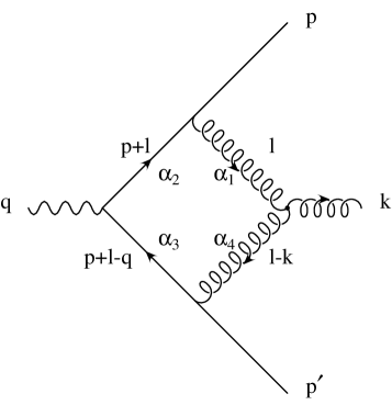
Figure B.1: Diagram representing $B_{2m}$.

We are referring, as far as the denominator structure is concerned, to a Feynman diagram of the type depicted in Fig. B.1

$$B_{2m}\equiv\int\frac{d^{d}l}{(2\pi)^{d}}\ \frac{1}{l^{2}}\ \frac{1}{(l-k)^{2}}\ \frac{1}{(l+p-q)^{2}-m^{2}}\ \frac{1}{(l+p)^{2}-m^{2}}\;.$$ (B.7)

Using eqs. (A.15) and (A.16), we can rewrite this integral as

$$B_{2m}=\frac{i}{16\pi^{2}}\ (4\pi)^{\epsilon}\ \Gamma(2+\epsilon)\int\frac{[d\alpha]}{D^{2+\epsilon}}\;,\quad\quad\quad d=4-2\epsilon\;,$$ (B.8)

where

$$D = {}-\left[\alpha_{1}\,\alpha_{2}\,m^{2}+\alpha_{1}\,\alpha_{3}\,(q-p)^{2}+\alpha_{2}\,\alpha_{3}\,q^{2}+\alpha_{2}\,\alpha_{4}\,(p+k)^{2}+\alpha_{3}\,\alpha_{4}\,m^{2}\right]$$ (B.9)

$${}+(\alpha_{2}+\alpha_{3})\,m^{2}-i\eta\;.$$

According to the definitions given in eqs. (B.1)–(B.6), $D$ becomes

$$D\!\! = \!\!-\left[m^{2}(\alpha_{1}\,\alpha_{2}+\alpha_{3}\,\alpha_{4}-\alpha_{2}-\alpha_{3})+s_{2}\,\alpha_{1}\,\alpha_{3}+q^{2}\alpha_{2}\,\alpha_{3}+s_{1}\,\alpha_{2}\,\alpha_{4}+i\eta\right]$$ (B.10)

$$= \!\!-\left[-m^{2}(\alpha_{2}+\alpha_{3})^{2}+(s_{2}-m^{2})\alpha_{1}\,\alpha_{3}+q^{2}\alpha_{2}\,\alpha_{3}+(s_{1}-m^{2})\alpha_{2}\,\alpha_{4}+i\eta\right]\;.\phantom{aaaa}$$

In order to perform the integration, it is useful to continue the denominator in a region where it is a negative-definite form. For this reason, we assume $m^{2}<0$, and we perform the integration of a function that now has no poles on the integration contour. At the end, we return to the physical region according to the $i\eta$ prescription

$$M^{2}\equiv-(m^{2}-i\eta)>0\;.$$ (B.11)

With this definition, we have

$$D=-\left[M^{2}(\alpha_{2}+\alpha_{3})^{2}+\sigma_{2}\,\alpha_{1}\,\alpha_{3}+q^{2}\alpha_{2}\,\alpha_{3}+\sigma_{1}\,\alpha_{2}\,\alpha_{4}\right]\;,$$ (B.12)

and eq. (B.8) becomes

$$B_{2m}=\frac{i}{16\pi^{2}}\ (4\pi)^{\epsilon}\ \Gamma(2+\epsilon)\ \frac{1}{(-1-i\eta)^{\epsilon}}\int\frac{[d\alpha]}{\left[-D\right]^{2+\epsilon}}=\frac{i}{16\pi^{2}}\ (4\pi)^{\epsilon}\ \Gamma(2+\epsilon)\ {\rm e}^{i\pi\epsilon}\,I\;.\phantom{aa}$$ (B.13)

We make the following change of variables

$$\begin{array}[]{l}\alpha_{1}=(1-y)z\\ \alpha_{2}=xy\\ \alpha_{3}=(1-x)y\\ \alpha_{4}=(1-y)(1-z)\;,\\ \end{array}$$ (B.14)

where the Jacobian of the transformation is

$$\frac{\partial(\alpha_{1}\,\alpha_{2}\,\alpha_{3})}{\partial(x\,y\,z)}=y(1-y)\;.$$

In this way, we can write $I$ of eq. (B.13) as

$$I\! = \!\int_{0}^{1}dx\,dy\,dz\ y\,(1-y)$$

$$\!{}\times\frac{1}{\Bigl{[}M^{2}y^{2}+\sigma_{2}yz(1-x)(1-y)+q^{2}xy^{2}(1-x)+\sigma_{1}xy(1-y)(1-z)\Bigr{]}^{2+\epsilon}}$$

$$= \!\int_{0}^{1}dx\,dy\,dz\ y^{-1-\epsilon}(1-y)$$

$$\!{}\times\frac{1}{\Bigl{\{}z\Bigl{[}\sigma_{2}(1-x)(1-y)-\sigma_{1}x(1-y)\Bigr{]}+M^{2}y+q^{2}xy(1-x)+\sigma_{1}x(1-y)\Bigr{\}}^{2+\epsilon}}\;.$$

The $z$ integration is easily done

$$I = \int_{0}^{1}dx\,dy\frac{1}{1+\epsilon}\ \frac{y^{-1-\epsilon}}{\sigma_{2}(1-x)-\sigma_{1}x}\left\{\frac{1}{\Bigl{[}M^{2}y+q^{2}xy(1-x)+\sigma_{1}x(1-y)\Bigr{]}^{1+\epsilon}}\right.$$ (B.15)

$$\left.{}-\frac{1}{\Bigl{[}\sigma_{2}(1-x)(1-y)+M^{2}y+q^{2}xy(1-x)\Bigr{]}^{1+\epsilon}}\right\}\;,$$

and, making the change of variable $x\rightarrow 1-x$ in the second integral, we have

$$I = \int_{0}^{1}dx\,dy\frac{-1}{1+\epsilon}\ \frac{y^{-1-\epsilon}}{\sigma_{2}x-\sigma_{1}(1-x)}\ \frac{1}{\Bigl{[}\sigma_{2}x(1-y)+M^{2}y+q^{2}xy(1-x)\Bigr{]}^{1+\epsilon}}$$

$${}+\int_{0}^{1}dx\,dy\frac{-1}{1+\epsilon}\ \frac{y^{-1-\epsilon}}{\sigma_{1}x-\sigma_{2}(1-x)}\ \frac{1}{\Bigl{[}\sigma_{1}x(1-y)+M^{2}y+q^{2}xy(1-x)\Bigr{]}^{1+\epsilon}}\;.$$

We then decompose $I$ as the sum of the two integrals

$$I=I_{1}(\sigma_{1},\sigma_{2})+I_{2}(\sigma_{1},\sigma_{2})\;,$$

which have the symmetry

$$I_{2}(\sigma_{1},\sigma_{2})=I_{1}(\sigma_{2},\sigma_{1})\;,$$

so that $I$ becomes

$$I=I_{1}(\sigma_{1},\sigma_{2})+I_{1}(\sigma_{2},\sigma_{1})\;,$$ (B.16)

and we have to perform only one integration

$$I_{1}=\int_{0}^{1}dx\,dy\frac{-1}{1+\epsilon}\ \frac{1}{\sigma_{2}x-\sigma_{1}(1-x)}\ \frac{1}{(\sigma_{2}x)^{1+\epsilon}}\ \frac{y^{-1-\epsilon}}{\left\{1+y\left[-1+\frac{M^{2}}{\sigma_{2}x}+\frac{q^{2}}{\sigma_{2}}(1-x)\right]\right\}^{1+\epsilon}}\;.$$

Using the identity (A.8)

$$I_{1} = \int_{0}^{1}dx\,dy\frac{-1}{1+\epsilon}\ \frac{1}{\sigma_{2}x-\sigma_{1}(1-x)}\ \frac{1}{(\sigma_{2}x)^{1+\epsilon}}\ \left(\frac{M^{2}}{\sigma_{2}x}+\frac{q^{2}}{\sigma_{2}}(1-x)\right)^{\epsilon}$$ (B.17)

$${}\times y^{-1-\epsilon}\,\left[1-y\frac{-x+\frac{M^{2}}{\sigma_{2}}+\frac{q^{2}}{\sigma_{2}}x(1-x)}{\frac{M^{2}}{\sigma_{2}}+\frac{q^{2}}{\sigma_{2}}x(1-x)}\right]^{2\epsilon}$$

$$= \frac{-1}{1+\epsilon}(M^{2})^{-\epsilon}\int_{0}^{1}dx\,dy\,\frac{1}{\sigma_{2}x-\sigma_{1}(1-x)}\ \frac{M^{2\epsilon}}{(\sigma_{2}x)^{1+2\epsilon}}\left[M^{2}+q^{2}x(1-x)\right]^{\epsilon}$$

$${}\times y^{-1-\epsilon}\,\Biggl{\{}\Biggl{(}1-y+y\,\frac{x}{\frac{M^{2}}{\sigma_{2}}+\frac{q^{2}}{\sigma_{2}}x(1-x)}\Biggr{)}^{2\epsilon}-(1-y)^{2\epsilon}{}+(1-y)^{2\epsilon}\Biggr{\}}\;,\phantom{aaaa}$$

where, in the curly braces, we have added and subtracted the same quantity. If we consider now the first two terms in the curly braces and expand them in $\epsilon$, we have

$$f(x,y) \equiv \Biggl{(}1-y+y\,\frac{x}{\frac{M^{2}}{\sigma_{2}}+\frac{q^{2}}{\sigma_{2}}x(1-x)}\Biggr{)}^{2\epsilon}-(1-y)^{2\epsilon}$$ (B.18)

$$= 2\,\epsilon\,\Biggl{\{}\log\Biggl{(}1-y+y\,\frac{x}{\frac{M^{2}}{\sigma_{2}}+\frac{q^{2}}{\sigma_{2}}x(1-x)}\Biggr{)}-\log(1-y)\Biggr{\}}+{\cal O}\left(\epsilon^{2}\right)\;.\phantom{aaaaa}$$

Since we are keeping only terms till order ${\cal O}\left(\epsilon^{0}\right)$, $f(x,y)$ gives contribution to the integral only if it is multiplied by factors at least of order $1/\epsilon$. Such factors may arise only at singular points, which, for eq. (B.17), are $x=0$ and $y=0$: in fact $f(x,y)$ is multiplied by $x^{-1-2\epsilon}y^{-1-\epsilon}$. In the limit $x\,\mbox{$\rightarrow$}\,0$, $y\,\mbox{$\rightarrow$}\,0$, we have

$$x^{-1-2\epsilon}y^{-1-\epsilon}f(x,y) = 2\,\epsilon\,x^{-1-2\epsilon}y^{-1-\epsilon}\Biggl{(}-y+y\,\frac{x}{\frac{M^{2}}{\sigma_{2}}+\frac{q^{2}}{\sigma_{2}}x(1-x)}+y+{\cal O}\left(xy^{2}\right)\Biggr{)}$$ (B.19)

$$\approx 2\,\epsilon\,x^{-2\epsilon}y^{-\epsilon}\frac{1}{\frac{M^{2}}{\sigma_{2}}+\frac{q^{2}}{\sigma_{2}}x(1-x)}\;,$$

that gives zero contribution in the limit $\epsilon\,\mbox{$\rightarrow$}\,0$. In this way, $f(x,y)$ gives no contributions and can be disregarded. By integrating eq. (B.17) in $y$, we obtain

$$I_{1} = \frac{(M^{2})^{-\epsilon}}{1+\epsilon}\ \frac{1}{\epsilon}\ F_{\epsilon}$$ (B.21)

$${}\times\int_{0}^{1}dx\ \frac{1}{\sigma_{2}x-\sigma_{1}(1-x)}\ \frac{1}{\sigma_{2}x}\ x^{-2\epsilon}\left(\frac{M^{2}}{\sigma_{2}}\right)^{2\epsilon}\left[1+\frac{q^{2}}{M^{2}}x(1-x)\right]^{\epsilon}$$

$$= \frac{(M^{2})^{-\epsilon}}{1+\epsilon}\ \frac{1}{\epsilon}\ \frac{F_{\epsilon}}{\sigma_{1}\sigma_{2}}$$

$${}\times\int_{0}^{1}dx\ \left[\frac{\sigma_{1}+\sigma_{2}}{\sigma_{2}x-\sigma_{1}(1-x)}-\frac{1}{x}\right]\left(\frac{M^{2}}{\sigma_{2}}\right)^{2\epsilon}x^{-2\epsilon}\left[1+\frac{q^{2}}{M^{2}}x(1-x)\right]^{\epsilon}$$

$$= \frac{(M^{2})^{-\epsilon}}{1+\epsilon}\ \frac{1}{\epsilon}\ \frac{F_{\epsilon}}{\sigma_{1}\sigma_{2}}\left\{\int_{0}^{1}dx\ \frac{\sigma_{1}+\sigma_{2}}{\sigma_{2}x-\sigma_{1}(1-x)}\left(1+2\epsilon\log\frac{M^{2}}{\sigma_{2}x}+{\cal O}\left(\epsilon^{2}\right)\right)\right.$$

$$\times\left[1+\epsilon\log\left(1+\frac{q^{2}}{M^{2}}x(1-x)\right)+{\cal O}\left(\epsilon^{2}\right)\right]$$

$$\left.{}-\int_{0}^{1}dx\ \left(\frac{M^{2}}{\sigma_{2}}\right)^{2\epsilon}\,x^{-1-2\epsilon}\left[1+\epsilon\log\left(1+\frac{q^{2}}{M^{2}}x(1-x)\right)+{\cal O}\left(\epsilon^{2}\right)\right]\right\}$$

$$= \frac{(M^{2})^{-\epsilon}}{1+\epsilon}\ \frac{1}{\epsilon}\ \frac{F_{\epsilon}}{\sigma_{1}\sigma_{2}}\ \Biggl{\{}\int_{0}^{1}dx\ \frac{\sigma_{1}+\sigma_{2}}{\sigma_{2}x-\sigma_{1}(1-x)}$$

$$\times\Biggl{[}\underbrace{1+\epsilon\log\Biggl{(}1+\frac{q^{2}}{M^{2}}x(1-x)\Biggr{)}}_{A_{1}}+2\epsilon\log\frac{M^{2}}{\sigma_{2}x}+{\cal O}\left(\epsilon^{2}\right)\Biggr{]}$$

$$-\left[1+2\epsilon\log\frac{M^{2}}{\sigma_{2}}+2\epsilon^{2}\log^{2}\frac{M^{2}}{\sigma_{2}}+{\cal O}\left(\epsilon^{3}\right)\right]$$

$$\times\Biggl{[}-\frac{1}{2\epsilon}+\epsilon\underbrace{\int_{0}^{1}dx\ x^{-1-2\epsilon}\log\Biggl{(}1+\frac{q^{2}}{M^{2}}x(1-x)\Biggr{)}}_{{\rm finite\ for\ }\epsilon\,\rightarrow\,0}+{\cal O}\left(\epsilon^{2}\right)\Biggr{]}\Biggr{\}}\;,$$

where

$$F_{\epsilon}=\frac{\Gamma(1-\epsilon)\,\Gamma(1+2\epsilon)}{\Gamma(1+\epsilon)}=1+\frac{\pi^{2}}{3}\epsilon^{2}+{\cal O}\left(\epsilon^{3}\right)\;.$$ (B.22)

The contribution given by $A_{1}$ to the total integral $I$ is zero. In fact, using eq. (B.16), we have

$$\int_{0}^{1}dx\ \frac{\sigma_{1}+\sigma_{2}}{\sigma_{2}x-\sigma_{1}(1-x)}A_{1}+\int_{0}^{1}dx\ \frac{\sigma_{2}+\sigma_{1}}{\sigma_{1}x-\sigma_{2}(1-x)}A_{1}=0\;,$$

and then

$$I_{1} = \frac{(M^{2})^{-\epsilon}}{1+\epsilon}\ \frac{F_{\epsilon}}{\sigma_{1}\sigma_{2}}\left\{-2(\sigma_{1}+\sigma_{2})\int_{0}^{1}dx\ \frac{\log\frac{\sigma_{2}x}{M^{2}}}{\sigma_{2}x-\sigma_{1}(1-x)}\right.$$ (B.23)

$${}-\int_{0}^{1}dx\ \frac{1}{x}\log\left(1+\frac{q^{2}}{M^{2}}x(1-x)\right)+\left.\frac{1}{2\epsilon^{2}}+\frac{1}{\epsilon}\log\frac{M^{2}}{\sigma_{2}}+\log^{2}\frac{M^{2}}{\sigma_{2}}\right\}\;.\phantom{aaaaa}$$

From eq. (B.16) we have

$$I = \frac{(M^{2})^{-\epsilon}}{1+\epsilon}\ \frac{F_{\epsilon}}{\sigma_{1}\sigma_{2}}$$ (B.24)

$${}\times\left\{-2(\sigma_{1}+\sigma_{2})\int_{0}^{1}dx\ \frac{\log\frac{\sigma_{2}x}{\sigma_{1}(1-x)}}{\sigma_{2}x-\sigma_{1}(1-x)}-2\int_{0}^{1}\frac{dx}{x}\log\left(1+\frac{q^{2}}{M^{2}}x(1-x)\right)\right.$$

$$\left.{}+\frac{1}{\epsilon^{2}}+\frac{1}{\epsilon}\left(\log\frac{M^{2}}{\sigma_{1}}+\log\frac{M^{2}}{\sigma_{2}}\right)+\log^{2}\frac{M^{2}}{\sigma_{1}}+\log^{2}\frac{M^{2}}{\sigma_{2}}\right\}\;.$$

In this way, we succeed in isolating all the divergent contributions, which have appeared as poles in $\epsilon$. The remaining integrals are finite. For the first integral in eq. (B.24) we have

$$\int_{0}^{1}dx\ \frac{\log\frac{\sigma_{2}x}{\sigma_{1}(1-x)}}{\sigma_{2}x-\sigma_{1}(1-x)}=\frac{1}{2\left(\sigma_{1}+\sigma_{2}\right)}\left(\log^{2}\frac{\sigma_{1}}{\sigma_{2}}+\pi^{2}\right)\;,$$

that can be demonstrated using the contour integrals around the poles $0,1$ and $\sigma_{1}/\left(\sigma_{1}+\sigma_{2}\right)$, and the identity

$$\log\left(\frac{\sigma_{2}}{\sigma_{1}}\frac{x}{1-x}\right)=\frac{1}{4\pi\,i}\left[\log^{2}\left.\left(-\frac{\sigma_{2}}{\sigma_{1}}\frac{x}{1-x}\right)\right|_{x-i\epsilon}-\log^{2}\left.\left(-\frac{\sigma_{2}}{\sigma_{1}}\frac{x}{1-x}\right)\right|_{x+i\epsilon}\right]\;.$$ (B.25)

The last integral in eq. (B.24) is solved with

$$\int_{0}^{1}\frac{dx}{x}\log\left[1+x(1-x)\frac{q^{2}}{M^{2}}\right] = \int_{0}^{1}\frac{dx}{x}\log\left(1-\frac{x}{\lambda_{+}}\right)+\int_{0}^{1}\frac{dx}{x}\log\left(1-\frac{x}{\lambda_{-}}\right)$$ (B.26)

$$= -\,{\rm Li}_{2}\left(\frac{1}{\lambda_{+}}\right)-\,{\rm Li}_{2}\left(\frac{1}{\lambda_{-}}\right)=\frac{1}{2}\log^{2}\left(1-\frac{1}{\lambda_{-}}\right)$$

$$= \frac{1}{2}\log^{2}\frac{-\lambda_{-}}{\lambda_{+}}\;,$$

where we have defined

$$\lambda_{\pm}=\frac{1}{2}\left(1\pm\sqrt{1+\frac{4M^{2}}{q^{2}}}\right)\equiv\frac{1}{2}\left(1\pm\Delta\right)$$ (B.27)

$$\lambda_{+}+\lambda_{-}=1\;.$$

The integral $I$ becomes

$$I = \frac{(M^{2})^{-\epsilon}}{1+\epsilon}\ \frac{F_{\epsilon}}{\sigma_{1}\sigma_{2}}\left\{-\left(\log^{2}\frac{\sigma_{1}}{\sigma_{2}}+\pi^{2}\right)-\log^{2}\left(1-\frac{1}{\lambda_{-}}\right)+\log^{2}\frac{M^{2}}{\sigma_{1}}+\log^{2}\frac{M^{2}}{\sigma_{2}}\right.$$ (B.28)

$$\left.{}+\frac{1}{\epsilon^{2}}+\frac{1}{\epsilon}\left(\log\frac{M^{2}}{\sigma_{1}}+\log\frac{M^{2}}{\sigma_{2}}\right)\right\}\;,$$

and, according to eq. (B.13),

$$B_{2m} = \frac{i}{16\pi^{2}}\ (4\pi)^{\epsilon}\ \Gamma(1+\epsilon)\ {\rm e}^{i\pi\epsilon}\ (M^{2})^{-\epsilon}\frac{1}{\sigma_{1}\sigma_{2}}\left\{\frac{1}{\epsilon^{2}}+\frac{1}{\epsilon}\left(\log\frac{M^{2}}{\sigma_{1}}+\log\frac{M^{2}}{\sigma_{2}}\right)\right.$$ (B.29)

$$\left.{}+2\log\left(\frac{M^{2}}{\sigma_{1}}\right)\log\left(\frac{M^{2}}{\sigma_{2}}\right)-\frac{2}{3}\pi^{2}-\log^{2}\left(1-\frac{1}{\lambda_{-}}\right)\right\}\;.$$

We return to the physical region with the analytic continuation of $B_{2m}$, that is, using eq. (B.11)

$$(M^{2})^{-\epsilon}=(m^{2})^{-\epsilon}{\rm e}^{-i\pi\epsilon}$$ (B.30)

$$\log M^{2}=\log\left(-m^{2}+i\eta\right)=\log m^{2}+i\pi$$ (B.31)

$$\lambda_{\pm}=\frac{1}{2}\left(1\pm\sqrt{1-\frac{4m^{2}}{q^{2}}}\right)\pm i\eta=\frac{1}{2}\left(1\pm\Delta\right)\pm i\eta\;.$$ (B.32)

You can see that

$$0\leq\lambda_{-}\leq 1/2\;,\quad\quad\quad\quad 1/2\leq\lambda_{+}\leq 1\;,$$ (B.33)

and then

$$\halign{\hbox to\displaywidth{$\hfil\displaystyle#\hfil$}\cr 0.0pt{\hfil$\displaystyle\quad 1-\frac{1}{\lambda_{-}}<0\longrightarrow 1-\frac{1}{\lambda_{-}}-i\eta\;,\hfill\crcr}}$$

so that the logarithm acquires an imaginary part

$$\halign{\hbox to\displaywidth{$\hfil\displaystyle#\hfil$}\cr 0.0pt{\hfil$\displaystyle\quad\log\left(1-\frac{1}{\lambda_{-}}\right)=-\log\frac{-\lambda_{-}}{\lambda_{+}}\longrightarrow\log\frac{\lambda_{+}}{\lambda_{-}}-i\pi\;.\hfill\crcr}}$$

The final result is

$$B_{2m} = N(\epsilon)\,\left(m^{2}\right)^{-\epsilon}\frac{1}{\sigma_{1}\sigma_{2}}\left\{\frac{1}{\epsilon^{2}}+\frac{1}{\epsilon}\left(\log\frac{m^{2}}{\sigma_{1}}+\log\frac{m^{2}}{\sigma_{2}}\right)+2\log\frac{m^{2}}{\sigma_{1}}\,\log\frac{m^{2}}{\sigma_{2}}\right.$$ (B.34)

$$\left.{}-\frac{5}{3}\pi^{2}-\log^{2}\frac{\lambda_{+}}{\lambda_{-}}+2\,\pi\,i\left[\frac{1}{\epsilon}+\log\frac{m^{2}}{\sigma_{1}}+\log\frac{m^{2}}{\sigma_{2}}+\log\frac{\lambda_{+}}{\lambda_{-}}\right]\right\}\;,$$

where

$${\rm N}(\epsilon)=\frac{i}{16\pi^{2}}\left(4\pi\right)^{\epsilon}\Gamma(1+\epsilon)\;.$$ (B.35)

B.3 Box with three massive propagators: $B_{3m}$

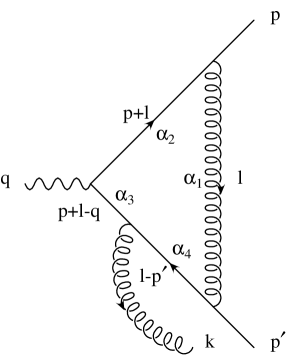
Figure B.2: Diagram representing $B_{3m}$.

We are referring, as far as the denominator structure is concerned, to a Feynman diagram of the type represented in Fig. B.2

$$B_{3m}\equiv\int\frac{d^{d}l}{(2\pi)^{d}}\ \frac{1}{l^{2}}\ \frac{1}{(l+p)^{2}-m^{2}}\ \frac{1}{(l+p-q)^{2}-m^{2}}\ \frac{1}{(l-p^{\prime})^{2}-m^{2}}\;.$$

Performing the same steps done for the calculation of $B_{2m}$, we have

$$B_{3m}=\frac{i}{16\pi^{2}}\ (4\pi)^{\epsilon}\ \Gamma(2+\epsilon)\int\frac{[d\alpha]}{D^{2+\epsilon}}\;,\quad\quad\quad d=4-2\epsilon\;,$$ (B.36)

where

$$D = -\left[\alpha_{1}\,\alpha_{2}\,m^{2}+\alpha_{1}\,\alpha_{3}\,(q-p)^{2}+\alpha_{1}\,\alpha_{4}\,m^{2}+\alpha_{2}\,\alpha_{3}\,q^{2}+\alpha_{2}\,\alpha_{4}\,(q-k)^{2}\right]$$ (B.37)

$$+(\alpha_{2}+\alpha_{3}+\alpha_{4})\,m^{2}-i\eta\;.$$

Using the definitions of the kinematical invariants of eqs. (B.1)–(B.6) and continuing the integral into the unphysical region of negative mass, according to eq. (B.11), we have

$$D = -\left[\alpha_{1}(\alpha_{2}+\alpha_{4})\,m^{2}+\alpha_{1}\,\alpha_{3}\,s_{2}+\alpha_{2}\,\alpha_{3}\,q^{2}+\alpha_{2}\,\alpha_{4}\,s_{3}-(1-\alpha_{1})\,m^{2}+i\eta\right]$$ (B.38)

$$= -\left[-m^{2}(1-\alpha_{1})^{2}+\sigma_{2}\,\alpha_{1}\,\alpha_{3}+q^{2}\,\alpha_{3}\,\alpha_{2}+s_{3}\,\alpha_{2}\,\alpha_{4}+i\eta\right]$$

$$= -\left[M^{2}(1-\alpha_{1})^{2}+\sigma_{2}\,\alpha_{1}\,\alpha_{3}+q^{2}\,\alpha_{2}\,\alpha_{3}+s_{3}\,\alpha_{2}\,\alpha_{4}\right]\;.$$

The integral (B.36) then becomes

$$B_{3m}=\frac{i}{16\pi^{2}}\ (4\pi)^{\epsilon}\ \Gamma(2+\epsilon)\ {\rm e}^{i\pi\epsilon}\int\frac{[d\alpha]}{\left[-D\right]^{2+\epsilon}}=(1+\epsilon)\,{\rm N}(\epsilon)\,{\rm e}^{i\pi\epsilon}\,I\;.$$ (B.39)

By making the following change of variables

$$\begin{array}[]{l}\alpha_{1}=1-x\\ \alpha_{2}=x(1-z)\\ \alpha_{3}=xyz\\ \alpha_{4}=x(1-y)z\;,\\ \end{array}$$ (B.40)

and taking into account the Jacobian of the transformation

$$\frac{\partial(\alpha_{1}\,\alpha_{2}\,\alpha_{3})}{\partial(x\,y\,z)}=x^{2}z\;,$$

we have

$$I = \int_{0}^{1}dx\,dy\,dz\,\frac{x^{2}z}{\Bigl{[}M^{2}x^{2}+\sigma_{2}(1-x)xyz+s_{3}x^{2}(1-y)z(1-z)+q^{2}x^{2}yz(1-z)\Bigr{]}^{2+\epsilon}}$$ (B.41)

$$= \int_{0}^{1}dx\,dy\,dz\,\frac{zx^{-\epsilon}}{\Bigl{[}M^{2}x+\sigma_{2}(1-x)yz+s_{3}x(1-y)z(1-z)+q^{2}xyz(1-z)\Bigr{]}^{2+\epsilon}}$$

$$= \int_{0}^{1}dx\,dz\,\frac{-1}{1+\epsilon}\ \frac{x^{-\epsilon}}{\sigma_{2}(1-x)-s_{3}x(1-z)+q^{2}x(1-z)}$$

$$\times\left[\frac{1}{\Bigl{[}M^{2}x+\sigma_{2}(1-x)z+q^{2}xz(1-z)\Bigr{]}^{1+\epsilon}}-\frac{1}{\Bigl{[}M^{2}x+s_{3}xz(1-z)\Bigr{]}^{1+\epsilon}}\right]$$

$$= -\frac{1}{1+\epsilon}\int_{0}^{1}dx\,dz\,\frac{1}{\sigma_{2}(1-x)+(q^{2}-s_{3})x(1-z)}$$

$$\times\left[\frac{x^{-\epsilon}}{\Bigl{[}M^{2}x+\sigma_{2}(1-x)z+q^{2}xz(1-z)\Bigr{]}^{1+\epsilon}}-\frac{x^{-1-2\epsilon}}{\Bigl{[}M^{2}+s_{3}z(1-z)\Bigr{]}^{1+\epsilon}}\right]\;.$$

When $x\,\mbox{$\rightarrow$}\,0$, the second integral is divergent: for this reason, we add and subtract the asymptotic expression of the divergent function when $x$ goes to zero

$$I\!\! = \!\!-\frac{1}{1+\epsilon}\left\{\int_{0}^{1}dx\,dz\,\frac{1}{\sigma_{2}(1-x)+(q^{2}-s_{3})x(1-z)}\phantom{\frac{x^{-\epsilon}}{\Bigl{[}M^{2}\Bigr{]}^{1+\epsilon}}}\right.$$ (B.42)

$$\!\!\times\left[\frac{x^{-\epsilon}}{\Bigl{[}M^{2}x+\sigma_{2}(1-x)z+q^{2}xz(1-z)\Bigr{]}^{1+\epsilon}}-\frac{x^{-1-2\epsilon}}{\Bigl{[}M^{2}+s_{3}z(1-z)\Bigr{]}^{1+\epsilon}}\right]$$

$$\!\!\left.+\int_{0}^{1}dx\,dz\,\frac{x^{-1-2\epsilon}}{\sigma_{2}\Bigl{[}M^{2}+s_{3}z(1-z)\Bigr{]}^{1+\epsilon}}-\int_{0}^{1}dx\,dz\,\frac{x^{-1-2\epsilon}}{\sigma_{2}\Bigl{[}M^{2}+s_{3}z(1-z)\Bigr{]}^{1+\epsilon}}\right\}\phantom{aaaaa}$$

We can make the following considerations:

1. the first term is finite when $\epsilon\,\mbox{$\rightarrow$}\,0$

2. the sum of the second and the third term is finite when $x\,\mbox{$\rightarrow$}\,0$ by construction, and then we can again put $\epsilon=0$

3. the integral of the last term is

   $$I_{L} \equiv \int_{0}^{1}dx\,dz\,\frac{x^{-1-2\epsilon}}{\sigma_{2}\,\Bigl{[}M^{2}+s_{3}z(1-z)\Bigr{]}^{1+\epsilon}}$$

   $$= -\frac{(M^{2})^{-\epsilon}}{2\,\sigma_{2}\,\epsilon}\int_{0}^{1}dz\,\frac{1}{M^{2}\Bigl{[}1+\frac{s_{3}}{M^{2}}z(1-z)\Bigr{]}^{1+\epsilon}}$$

   $$= -\frac{(M^{2})^{-\epsilon}}{2\,\sigma_{2}\,\epsilon}\int_{0}^{1}dz\,\frac{1}{M^{2}+s_{3}z(1-z)}+\frac{1}{2\,\sigma_{2}}\int_{0}^{1}dz\,\frac{\log\left[1+\frac{s_{3}}{M^{2}}z(1-z)\right]}{M^{2}+s_{3}z(1-z)}\;.$$

By collecting a global factor $(M^{2})^{-\epsilon}$, eq. (B.42) becomes

$$I = -\frac{(M^{2})^{-\epsilon}}{1+\epsilon}\left\{\int_{0}^{1}dx\,dz\,\left[\frac{1}{\sigma_{2}(1-x)+(q^{2}-s_{3})x(1-z)}\phantom{\frac{1}{\Bigl{[}M^{2}}}\right.\right.$$ (B.44)

$$\times\left(\frac{1}{M^{2}x+\sigma_{2}(1-x)z+q^{2}xz(1-z)}-\frac{1}{x\,\Bigl{[}M^{2}+s_{3}z(1-z)\Bigr{]}}\right)$$

$$+\left.\frac{1}{\sigma_{2}\,x\,\Bigl{[}M^{2}+s_{3}z(1-z)\Bigr{]}}\right]$$

$$+\left.\frac{1}{2\,\sigma_{2}\,\epsilon}\int_{0}^{1}dz\,\frac{1}{M^{2}+s_{3}z(1-z)}-\frac{1}{2\,\sigma_{2}}\int_{0}^{1}dz\,\frac{\log\left[1+\frac{s_{3}}{M^{2}}z(1-z)\right]}{M^{2}+s_{3}z(1-z)}\right\}$$

$$= -\frac{(M^{2})^{-\epsilon}}{1+\epsilon}\left\{\int_{0}^{1}dx\,dz\,\frac{M^{2}-\sigma_{2}z+q^{2}z(1-z)}{\sigma_{2}\,\Bigl{[}M^{2}+s_{3}z(1-z)\Bigr{]}\,\Bigl{[}M^{2}x+\sigma_{2}(1-x)z+q^{2}xz(1-z)\Bigr{]}}\right.$$

$$+\left.\frac{1}{2\,\sigma_{2}\,\epsilon}\int_{0}^{1}dz\,\frac{1}{M^{2}+s_{3}z(1-z)}-\frac{1}{2\,\sigma_{2}}\int_{0}^{1}dz\,\frac{\log\left[1+\frac{s_{3}}{M^{2}}z(1-z)\right]}{M^{2}+s_{3}z(1-z)}\right\}\;.$$

The integration in $x$ gives

$$I = -\frac{(M^{2})^{-\epsilon}}{1+\epsilon}\frac{1}{\sigma_{2}}\int_{0}^{1}dz\frac{1}{M^{2}+s_{3}z(1-z)}\Bigg{\{}\log\frac{M^{2}+q^{2}z(1-z)}{\sigma_{2}z}$$ (B.45)

$$+\frac{1}{2\epsilon}-\frac{1}{2}\log\left[1+\frac{s_{3}}{M^{2}}z(1-z)\right]\Bigg{\}}\;,$$

and decomposing the denominator

$$\frac{1}{M^{2}+s_{3}z(1-z)}=-\frac{1}{s_{3}\Delta^{\prime}}\left[\frac{1}{z-\xi_{+}}-\frac{1}{z-\xi_{-}}\right]\;,$$

where

$$\Delta^{\prime}=\sqrt{1+\frac{4M^{2}}{s_{3}}}\;,\quad\quad\quad\quad\xi_{\pm}=\frac{1}{2}\left[1\pm\Delta^{\prime}\right]\;,$$

and

$$\xi_{+}+\xi_{-}=1\;,$$

we have

$$I = \frac{(M^{2})^{-\epsilon}}{1+\epsilon}\frac{1}{\sigma_{2}s_{3}\Delta^{\prime}}\int_{0}^{1}dz\,\left[\frac{1}{z-\xi_{+}}-\frac{1}{z-\xi_{-}}\right]\Biggl{\{}\left(\frac{1}{2\epsilon}+\log\frac{q^{2}}{\sigma_{2}}-\frac{1}{2}\log\frac{s_{3}}{M^{2}}\right)$$ (B.46)

$$-\log z+\log(z-\lambda_{-})+\log(\lambda_{+}-z)-\frac{1}{2}\log(z-\xi_{-})-\frac{1}{2}\log(\xi_{+}-z)\Biggr{\}}\;,\phantom{aaaaa}$$

where $\lambda_{\pm}$ are given by eq. (B.27).

In order to compute these integrals, it is worth noticing that

$$\xi_{-}\leq\lambda_{-}\leq 0<1\leq\xi_{+}\leq\lambda_{+}\;,$$

where we have used the fact that $q^{2}\geq s_{3}$ (see eq. (B.3)). In addition

$$\halign{\hbox to\displaywidth{$\hfil\displaystyle#\hfil$}\cr 0.0pt{\hfil$\displaystyle\quad\int_{0}^{1}dz\,\left[\frac{1}{z-\xi_{+}}-\frac{1}{z-\xi_{-}}\right]=2\log\frac{-\xi_{-}}{\xi_{+}}\hfill\crcr}}$$

$$\halign{\hbox to\displaywidth{$\hfil\displaystyle#\hfil$}\cr 0.0pt{\hfil$\displaystyle\quad\int_{0}^{1}dz\,\frac{\log z}{z-\xi_{\pm}}=\,{\rm Li}_{2}\left(\frac{1}{\xi_{\pm}}\right)\hfill\crcr}}$$

$$\halign{\hbox to\displaywidth{$\hfil\displaystyle#\hfil$}\cr 0.0pt{\hfil$\displaystyle\quad\int_{0}^{1}dz\,\frac{\log(z-\xi_{-})}{z-\xi_{+}}=-\int_{0}^{1}dz\,\frac{\log(\xi_{+}-z)}{z-\xi_{-}}\hfill\cr 0.0pt{\hfil$\displaystyle\quad\phantom{\int_{0}^{1}dz\,\frac{\log(z-\xi_{-})}{z-\xi_{+}}}=\log\Delta^{\prime}\log\frac{-\xi_{-}}{\xi_{+}}-\,{\rm Li}_{2}\left(\frac{-\xi_{-}}{\Delta^{\prime}}\right)+\,{\rm Li}_{2}\left(\frac{\xi_{+}}{\Delta^{\prime}}\right)\hfill\crcr}}}$$

$$\halign{\hbox to\displaywidth{$\hfil\displaystyle#\hfil$}\cr 0.0pt{\hfil$\displaystyle\quad\int_{0}^{1}dz\,\frac{\log(z-\xi_{-})}{z-\xi_{-}}\stackrel{{\scriptstyle\rm B.P.}}{{=}}\frac{1}{2}\log^{2}(\xi_{+})-\frac{1}{2}\log^{2}(-\xi_{-})\hfill\crcr}}$$

$$\halign{\hbox to\displaywidth{$\hfil\displaystyle#\hfil$}\cr 0.0pt{\hfil$\displaystyle\quad\int_{0}^{1}dz\,\frac{\log(\xi_{+}-z)}{z-\xi_{+}}\stackrel{{\scriptstyle\rm B.P.}}{{=}}\frac{1}{2}\log^{2}(-\xi_{-})-\frac{1}{2}\log^{2}(\xi_{+})\hfill\crcr}}$$

$$\halign{\hbox to\displaywidth{$\hfil\displaystyle#\hfil$}\cr 0.0pt{\hfil$\displaystyle\quad\int_{0}^{1}dz\,\frac{\log(z-\lambda_{-})}{z-\xi_{-}}=\log\lambda_{+}\log\frac{\xi_{+}}{\eta_{-}}-\log(-\lambda_{-})\log\frac{-\xi_{-}}{\eta_{-}}-\,{\rm Li}_{2}\left(\frac{\lambda_{-}}{\eta_{-}}\right)+\,{\rm Li}_{2}\left(\frac{-\lambda_{+}}{\eta_{-}}\right)\hfill\crcr}}$$

$$\halign{\hbox to\displaywidth{$\hfil\displaystyle#\hfil$}\cr 0.0pt{\hfil$\displaystyle\quad\int_{0}^{1}dz\,\frac{\log(z-\lambda_{-})}{z-\xi_{+}}=\log\eta_{+}\log{\frac{-\xi_{-}}{\xi_{+}}}+\,{\rm Li}_{2}\left(\frac{\xi_{+}}{\eta_{+}}\right)-\,{\rm Li}_{2}\left(\frac{-\xi_{-}}{\eta_{+}}\right)\hfill\crcr}}$$

$$\halign{\hbox to\displaywidth{$\hfil\displaystyle#\hfil$}\cr 0.0pt{\hfil$\displaystyle\quad\int_{0}^{1}dz\,\frac{\log(\lambda_{+}-z)}{z-\xi_{-}}\stackrel{{\scriptstyle\rm B.P.}}{{=}}\log\xi_{+}\log(-\lambda_{-})-\log(-\xi_{-})\log\lambda_{+}-\int_{0}^{1}dz\,\frac{\log(z-\xi_{-})}{z-\lambda_{+}}\hfill\cr 0.0pt{\hfil$\displaystyle\quad\phantom{\int_{0}^{1}dz\,\frac{\log(\lambda_{+}-z)}{z-\xi_{-}}}\stackrel{{\scriptstyle\phantom{\rm B.P.}}}{{=}}\log\xi_{+}\log(-\lambda_{-})-\log(-\xi_{-})\log\lambda_{+}\hfill\cr 0.0pt{\hfil$\displaystyle\quad\phantom{\int_{0}^{1}dz\,\frac{\log(z-\xi_{-})}{z-\lambda_{+}}\stackrel{{\scriptstyle\rm B.P.}}{{=}}}-\left[\log\eta_{+}\log\frac{-\lambda_{-}}{\lambda_{+}}+\,{\rm Li}_{2}\left(\frac{\lambda_{+}}{\eta_{+}}\right)-\,{\rm Li}_{2}\left(\frac{-\lambda_{-}}{\eta_{+}}\right)\right]\hfill\crcr}}}}$$

$$\halign{\hbox to\displaywidth{$\hfil\displaystyle#\hfil$}\cr 0.0pt{\hfil$\displaystyle\quad\int_{0}^{1}dz\,\frac{\log(\lambda_{+}-z)}{z-\xi_{+}}\stackrel{{\scriptstyle\rm B.P.}}{{=}}\log(-\xi_{-})\log(-\lambda_{-})-\log\xi_{+}\log\lambda_{+}-\int_{0}^{1}dz\,\frac{\log(\xi_{+}-z)}{z-\lambda_{+}}\hfill\cr 0.0pt{\hfil$\displaystyle\quad\phantom{\int_{0}^{1}dz\,\frac{\log(\lambda_{+}-z)}{z-\xi_{+}}}\stackrel{{\scriptstyle\phantom{\rm B.P.}}}{{=}}\log(-\xi_{-})\log(-\lambda_{-})-\log\xi_{+}\log\lambda_{+}\hfill\cr 0.0pt{\hfil$\displaystyle\quad\phantom{\int_{0}^{1}dz\,\frac{\log(\lambda_{+}-z)}{z-\xi_{+}}\stackrel{{\scriptstyle\rm B.P.}}{{=}}}-\left[\log\eta_{-}\log\frac{-\lambda_{-}}{\lambda_{+}}+\,{\rm Li}_{2}\left(\frac{-\lambda_{+}}{\eta_{-}}\right)-\,{\rm Li}_{2}\left(\frac{\lambda_{-}}{\eta_{-}}\right)\right]\;,\hfill\crcr}}}}$$

where

$$\eta_{\pm}\equiv\frac{1}{2}(\Delta^{\prime}\pm\Delta)\;,$$

and B.P. means integration “By Parts”. The integral $I$ then becomes

$$I = \frac{(M^{2})^{-\epsilon}}{1+\epsilon}\frac{1}{\sigma_{2}s_{3}\Delta^{\prime}}\left\{\left(\frac{1}{\epsilon}+2\log\frac{q^{2}}{\sigma_{2}}+\log\frac{M^{2}}{s_{3}}\right)\log\frac{-\xi_{-}}{\xi_{+}}\right.$$ (B.47)

$${}-\,{\rm Li}_{2}\left(\frac{1}{\xi_{+}}\right)+\,{\rm Li}_{2}\left(\frac{1}{\xi_{-}}\right)+\,{\rm Li}_{2}\left(\frac{\xi_{+}}{\eta_{+}}\right)-\,{\rm Li}_{2}\left(\frac{-\xi_{-}}{\eta_{+}}\right)$$

$${}+2\log\lambda_{+}\log\eta_{-}-2\log(-\lambda_{-})\log\eta_{-}+2\,{\rm Li}_{2}\left(\frac{\lambda_{-}}{\eta_{-}}\right)-2\,{\rm Li}_{2}\left(\frac{-\lambda_{+}}{\eta_{-}}\right)$$

$${}+2\log(-\xi_{-})\log(-\lambda_{-})-2\log\xi_{+}\log\lambda_{+}-\log\xi_{+}\log(-\lambda_{-})+\log(-\xi_{-})\log\lambda_{+}$$

$${}+\,{\rm Li}_{2}\left(\frac{\lambda_{+}}{\eta_{+}}\right)-\,{\rm Li}_{2}\left(\frac{-\lambda_{-}}{\eta_{+}}\right)-\log\Delta^{\prime}\log\frac{-\xi_{-}}{\xi_{+}}+\,{\rm Li}_{2}\left(\frac{-\xi_{-}}{\Delta^{\prime}}\right)-\,{\rm Li}_{2}\left(\frac{\xi_{+}}{\Delta^{\prime}}\right)$$

$${}+\left.\frac{1}{2}\log^{2}\xi_{+}-\frac{1}{2}\log^{2}(-\xi_{-})+\log\eta_{+}\log\left(\frac{-\xi_{-}}{\xi_{+}}\frac{-\lambda_{-}}{\lambda_{+}}\right)\right\}\;.$$

We can use the following algebraic relations

$$\halign{\hbox to\displaywidth{$\hfil\displaystyle#\hfil$}\cr 0.0pt{\hfil$\displaystyle\quad\frac{\xi_{+}}{\eta_{+}}=\frac{1+\Delta^{\prime}}{\Delta^{\prime}+\Delta}=\frac{1+\Delta^{\prime}+\Delta-\Delta}{\Delta^{\prime}+\Delta}=\frac{\lambda_{-}}{\eta_{+}}+1\hfill\crcr}}$$

$$\halign{\hbox to\displaywidth{$\hfil\displaystyle#\hfil$}\cr 0.0pt{\hfil$\displaystyle\quad-\frac{\xi_{-}}{\eta_{+}}=1-\frac{\lambda_{+}}{\eta_{+}}\;,\hfill\crcr}}$$

and some properties of the dilogarithm function

$$\halign{\hbox to\displaywidth{$\hfil\displaystyle#\hfil$}\cr 0.0pt{\hfil$\displaystyle\quad\,{\rm Li}_{2}\left(\frac{\xi_{+}}{\Delta^{\prime}}\right)=-\,{\rm Li}_{2}\left(-\frac{-\xi_{-}}{\Delta^{\prime}}\right)-\log\frac{\xi_{+}}{\Delta^{\prime}}\log\frac{-\xi_{-}}{\Delta^{\prime}}+\frac{\pi^{2}}{6}\hfill\crcr}}$$

$$\halign{\hbox to\displaywidth{$\hfil\displaystyle#\hfil$}\cr 0.0pt{\hfil$\displaystyle\quad\,{\rm Li}_{2}\left(\frac{\lambda_{+}}{\eta_{+}}\right)-\,{\rm Li}_{2}\left(-\frac{\xi_{-}}{\eta_{+}}\right)=2\,{\rm Li}_{2}\left(\frac{\lambda_{+}}{\eta_{+}}\right)+\log\frac{\lambda_{+}}{\eta_{+}}\log\frac{-\xi_{-}}{\eta_{+}}-\frac{\pi^{2}}{6}\hfill\crcr}}$$

$$\halign{\hbox to\displaywidth{$\hfil\displaystyle#\hfil$}\cr 0.0pt{\hfil$\displaystyle\quad\,{\rm Li}_{2}\left(\frac{\xi_{+}}{\eta_{+}}\right)-\,{\rm Li}_{2}\left(-\frac{\lambda_{-}}{\eta_{+}}\right)=-2\,{\rm Li}_{2}\left(-\frac{\lambda_{-}}{\eta_{+}}\right)-\log\frac{-\lambda_{-}}{\eta_{+}}\log\frac{\xi_{+}}{\eta_{+}}+\frac{\pi^{2}}{6}\hfill\crcr}}$$

$$\halign{\hbox to\displaywidth{$\hfil\displaystyle#\hfil$}\cr 0.0pt{\hfil$\displaystyle\quad\,{\rm Li}_{2}\left(\frac{1}{\xi_{-}}\right)-\,{\rm Li}_{2}\left(\frac{1}{\xi_{+}}\right)=2\,{\rm Li}_{2}\left(\frac{1}{\xi_{-}}\right)+\frac{1}{2}\log^{2}\frac{-\xi_{-}}{\xi_{+}}\;,\hfill\crcr}}$$

to obtain

$$I = \frac{(M^{2})^{-\epsilon}}{1+\epsilon}\frac{1}{\sigma_{2}s_{3}\Delta^{\prime}}\left\{\frac{1}{\epsilon}\log\frac{-\xi_{-}}{\xi_{+}}+\left(2\log\frac{M^{2}}{\sigma_{2}}+\log\frac{M^{2}}{s_{3}}\right)\log\frac{-\xi_{-}}{\xi_{+}}\right.$$ (B.48)

$${}+2\,{\rm Li}_{2}\left(\frac{1}{\xi_{-}}\right)-2\,{\rm Li}_{2}\left(-\frac{\lambda_{-}}{\eta_{+}}\right)+2\,{\rm Li}_{2}\left(\frac{\lambda_{+}}{\eta_{+}}\right)+2\,{\rm Li}_{2}\left(\frac{\lambda_{-}}{\eta_{-}}\right)$$

$${}-2\,{\rm Li}_{2}\left(-\frac{\lambda_{+}}{\eta_{-}}\right)+2\,{\rm Li}_{2}\left(-\frac{\xi_{-}}{\Delta^{\prime}}\right)-\frac{\pi^{2}}{6}-2\log\eta_{-}\log\frac{-\lambda_{-}}{\lambda_{+}}$$

$$\left.{}+2\log\eta_{+}\log\frac{-\lambda_{-}}{\lambda_{+}}+\log^{2}\xi_{+}-2\log\Delta^{\prime}\log(-\xi_{-})+\log^{2}\Delta^{\prime}\right\}\;.$$

To return to the physical region, we must continue analytically the solution, using eqs. (B.30)–(B.32) and

$$\xi_{\pm}=\frac{1}{2}\left(1\pm\sqrt{1-\frac{4m^{2}}{s_{3}}}\right)\pm i\eta=\frac{1}{2}\left(1\pm\Delta^{\prime}\right)\pm i\eta\;.$$ (B.49)

You can see that

$$0\leq\lambda_{-},\xi_{-}\leq 1/2\;,\quad\quad\quad\quad 1/2\leq\lambda_{+},\xi_{+}\leq 1\;,$$ (B.50)

and then

$$\halign{\hbox to\displaywidth{$\hfil\displaystyle#\hfil$}\cr 0.0pt{\hfil$\displaystyle\quad\frac{1}{\xi_{-}}>1\longrightarrow\frac{1}{\xi_{-}}+i\eta\hfill\crcr}}$$

$$\halign{\hbox to\displaywidth{$\hfil\displaystyle#\hfil$}\cr 0.0pt{\hfil$\displaystyle\quad-\frac{\xi_{-}}{\xi_{+}}=-\frac{1-\Delta^{\prime}}{1+\Delta^{\prime}}<0\longrightarrow-\frac{1-\Delta^{\prime}-\frac{2}{s_{3}}\frac{1}{\Delta^{\prime}}i\eta}{1+\Delta^{\prime}+\frac{2}{s_{3}}\frac{1}{\Delta^{\prime}}i\eta}\hfill\cr 0.0pt{\hfil$\displaystyle\quad\phantom{-\frac{\xi_{-}}{\xi_{+}}}=-\frac{1-\Delta^{\prime}}{1+\Delta^{\prime}}+\underbrace{\frac{1-\Delta^{\prime}}{1+\Delta^{\prime}}\left(\frac{1}{1-\Delta^{\prime}}+\frac{1}{1+\Delta^{\prime}}\right)}_{>0}i\eta=-\frac{\xi_{-}}{\xi_{+}}+i\eta\;.\hfill\crcr}}}$$

In a similar way, you can demonstrate that

$$\halign{\hbox to\displaywidth{$\hfil\displaystyle#\hfil$}\cr 0.0pt{\hfil$\displaystyle\quad-\frac{\lambda_{-}}{\lambda_{+}}\longrightarrow-\frac{\lambda_{-}}{\lambda_{+}}+i\eta\;,\hfill\crcr}}$$

and

$$\halign{\hbox to\displaywidth{$\hfil\displaystyle#\hfil$}\cr 0.0pt{\hfil$\displaystyle\quad\frac{\lambda_{+}}{\eta_{+}}=\frac{1+\Delta}{\Delta^{\prime}+\Delta}>1\longrightarrow\frac{1+\Delta+\frac{2}{q^{2}}\frac{1}{\Delta}i\eta}{\Delta^{\prime}+\Delta+i\eta\left(\frac{2}{q^{2}}\frac{1}{\Delta}+\frac{2}{s_{3}}\frac{1}{\Delta^{\prime}}\right)}\hfill\cr 0.0pt{\hfil$\displaystyle\quad\phantom{\frac{\lambda_{+}}{\eta_{+}}}=\underbrace{\frac{1+\Delta}{\Delta^{\prime}+\Delta}}_{>0}\Biggl{[}1+i\eta\underbrace{\Biggl{(}\frac{1}{1+\Delta}-\frac{1+\frac{q^{2}}{s_{3}}\frac{\Delta}{\Delta^{\prime}}}{\Delta^{\prime}+\Delta}\Biggr{)}}_{<0}\Biggr{]}=\frac{\lambda_{+}}{\eta_{+}}-i\eta\hfill\crcr}}}$$

$$\halign{\hbox to\displaywidth{$\hfil\displaystyle#\hfil$}\cr 0.0pt{\hfil$\displaystyle\quad-\frac{\lambda_{+}}{\eta_{-}}\longrightarrow-\frac{\lambda_{+}}{\eta_{-}}+i\eta\hfill\crcr}}$$

$$\halign{\hbox to\displaywidth{$\hfil\displaystyle#\hfil$}\cr 0.0pt{\hfil$\displaystyle\quad\eta_{-}\longrightarrow\eta_{-}+i\eta\;.\hfill\crcr}}$$

Using eqs. (A.6) and (A.7) we can write $B_{3m}$ as

$$B_{3m} = N(\epsilon)\ (m^{2})^{-\epsilon}\frac{1}{\sigma_{2}s_{3}\Delta^{\prime}}\left\{\frac{1}{\epsilon}\log\frac{\xi_{-}}{\xi_{+}}+\left(2\log\frac{m^{2}}{\sigma_{2}}+\log\frac{m^{2}}{s_{3}}\right)\log\frac{\xi_{-}}{\xi_{+}}\right.$$ (B.51)

$${}-2\,{\rm Li}_{2}\left(\xi_{-}\right)-\log^{2}\xi_{-}-2\,{\rm Li}_{2}\left(-\frac{\lambda_{-}}{\eta_{+}}\right)-2\,{\rm Li}_{2}\left(\frac{\eta_{+}}{\lambda_{+}}\right)-\log^{2}\frac{\lambda_{+}}{\eta_{+}}$$

$${}+2\,{\rm Li}_{2}\left(\frac{\lambda_{-}}{\eta_{-}}\right)+2\,{\rm Li}_{2}\left(-\frac{\eta_{-}}{\lambda_{+}}\right)+\log^{2}\left(-\frac{\lambda_{+}}{\eta_{-}}\right)+2\,{\rm Li}_{2}\left(-\frac{\xi_{-}}{\Delta^{\prime}}\right)-\frac{\pi^{2}}{2}$$

$${}+2\log\left(-\frac{\eta_{+}}{\eta_{-}}\right)\log\frac{\lambda_{-}}{\lambda_{+}}+\log^{2}\xi_{+}-2\log\Delta^{\prime}\log\xi_{-}+\log^{2}\Delta^{\prime}$$

$$\left.{}+i\,\pi\left[\frac{1}{\epsilon}+2\log\frac{q^{2}}{\sigma_{2}}+4\log\eta_{+}-2\log\Delta^{\prime}+2\log\frac{\xi_{-}}{\xi_{+}}\right]\right\}\;.$$

B.4 First triangle with two massive propagators: $T_{2m}^{q}$

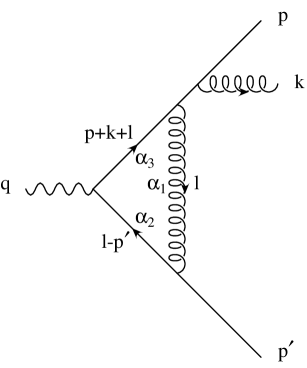
Figure B.3: Diagram representing $T_{2m}^{q}$.

We are referring, as far as the denominator structure is concerned, to a Feynman diagram of the type illustrated in Fig. B.3

$$T_{2m}^{q}\equiv\int\frac{d^{d}l}{(2\pi)^{d}}\ \frac{1}{l^{2}}\ \frac{1}{(l-p^{\prime})^{2}-m^{2}}\ \frac{1}{(l+p+k)^{2}-m^{2}}\;.$$ (B.52)

Using eqs. (A.15) and (A.16) we can write

$$T_{2m}^{q}=\frac{i}{16\pi^{2}}\ (4\pi)^{\epsilon}\ \Gamma(1+\epsilon)(-1)\int\frac{[d\alpha]}{D^{1+\epsilon}}\;,\quad\quad\quad d=4-2\epsilon\;,$$ (B.53)

where, with the help of eqs. (B.1)–(B.6),

$$D = -\left[\alpha_{1}\,\alpha_{2}\,m^{2}+\alpha_{1}\,\alpha_{3}(p+k)^{2}+\alpha_{2}\,\alpha_{3}\,q^{2}\right]+(\alpha_{2}+\alpha_{3})\,m^{2}-i\eta$$ (B.54)

$$= -\left[\alpha_{1}\,\alpha_{2}\,m^{2}+\alpha_{1}\,\alpha_{3}\,s_{1}+\alpha_{2}\,\alpha_{3}\,q^{2}-(\alpha_{2}+\alpha_{3})\,m^{2}+i\eta\right]$$

$$= -\left[-m^{2}(1-\alpha_{1})^{2}+\sigma_{1}\,\alpha_{1}\,\alpha_{3}+q^{2}\alpha_{2}\,\alpha_{3}+i\eta\right]\;.$$

Continuing the integral into the unphysical region, according to eq. (B.11), we have

$$D=-\left[M^{2}(1-\alpha_{1})^{2}+\sigma_{1}\,\alpha_{1}\,\alpha_{3}+q^{2}\alpha_{2}\,\alpha_{3}\right]\;.$$ (B.55)

The integral (B.53) then becomes

$$T_{2m}^{q}=\frac{i}{16\pi^{2}}\ (4\pi)^{\epsilon}\ \Gamma(1+\epsilon)\ {\rm e}^{i\pi\epsilon}\int\frac{[d\alpha]}{\left[-D\right]^{1+\epsilon}}={\rm N}(\epsilon)\,{\rm e}^{i\pi\epsilon}\,I\;.$$ (B.56)

The following change of variables

$$\begin{array}[]{l}\alpha_{1}=1-x\\ \alpha_{2}=x(1-y)\\ \alpha_{3}=xy\;,\\ \end{array}$$

together with the Jacobian of the transformation

$$\frac{\partial(\alpha_{1}\,\alpha_{2})}{\partial(x\,y)}=x\;,$$

gives

$$I = \int_{0}^{1}dx\,dy\,\frac{x}{\Bigl{[}M^{2}x^{2}+\sigma_{1}x(1-x)y+q^{2}x^{2}y(1-y)\Bigr{]}^{1+\epsilon}}$$ (B.57)

$$= \int_{0}^{1}dx\,dy\,\frac{x^{-\epsilon}}{\Bigl{[}M^{2}x+\sigma_{1}(1-x)y+q^{2}xy(1-y)\Bigr{]}^{1+\epsilon}}\;.$$

The integral $I$ is finite when $\epsilon\,\mbox{$\rightarrow$}\,0$, as can be seen also by inspecting eq. (B.52), that has no soft or collinear divergences. For this reason we put $\epsilon=0$ and integrate in $x$ to obtain

$$I=\int_{0}^{1}dy\frac{1}{M^{2}-\sigma_{1}y+q^{2}y(1-y)}\log\frac{M^{2}+q^{2}y(1-y)}{\sigma_{1}y}\;.$$ (B.58)

By decomposing the denominator in the following way

$$\frac{1}{M^{2}-\sigma_{1}y+q^{2}y(1-y)} = \frac{1}{-q^{2}\left[y^{2}-\left(1-\frac{\sigma_{1}}{q^{2}}\right)-\frac{M^{2}}{q^{2}}\right]}$$ (B.59)

$$= -\frac{1}{q^{2}}\frac{1}{\sqrt{\alpha_{1}^{2}+\frac{4M^{2}}{q^{2}}}}\left(\frac{1}{y-\rho_{+}}-\frac{1}{y-\rho_{-}}\right)\;,$$

where

$$\alpha_{1}\equiv 1-\frac{\sigma_{1}}{q^{2}}\;,\quad\quad\quad\quad\sqrt{\frac{4m^{2}}{q^{2}}}\leq\alpha_{1}\leq 1\;,$$

$$\rho_{\pm}=\frac{1}{2}\left[\alpha_{1}\pm\sqrt{\alpha_{1}^{2}+\frac{4M^{2}}{q^{2}}}\right]\;,$$

we have

$$I=\int_{0}^{1}dy\frac{-1}{q^{2}\sqrt{\alpha_{1}^{2}+\frac{4M^{2}}{q^{2}}}}\left(\frac{1}{y-\rho_{+}}-\frac{1}{y-\rho_{-}}\right)\log\left[\frac{-q^{2}}{\sigma_{1}}\frac{(y-\lambda_{+})(y-\lambda_{-})}{y}\right]\;.$$ (B.60)

It is easy to see that

$$\rho_{-}<\lambda_{-}<0<\rho_{+}<1<\lambda_{+}\;,$$ (B.61)

and $I$ becomes

$$I = -\frac{1}{q^{2}\sqrt{\alpha_{1}^{2}+\frac{4M^{2}}{q^{2}}}}\left\{\int_{0}^{1}dy\,\frac{1}{y-\rho_{+}}\left[\log\frac{\lambda_{+}-y}{\lambda_{+}-\rho_{+}}+\log\frac{y-\lambda_{-}}{\rho_{+}-\lambda_{-}}-\log\frac{y}{\rho_{+}}\right]\right.$$ (B.62)

$$\left.{}-\int_{0}^{1}dy\,\frac{1}{y-\rho_{-}}\left[\log\frac{\lambda_{+}-y}{\lambda_{+}-\rho_{-}}+\log\frac{y-\lambda_{-}}{\lambda_{-}-\rho_{-}}-\log\frac{y}{-\rho_{-}}\right]\right\}\;.$$

We summarize here the results of the integration in $y$

$$\halign{\hbox to\displaywidth{$\hfil\displaystyle#\hfil$}\cr 0.0pt{\hfil$\displaystyle\quad\int_{0}^{1}dy\frac{1}{y-\rho_{+}}\log\frac{\lambda_{+}-y}{\lambda_{+}-\rho_{+}}=\,{\rm Li}_{2}\left(-\frac{\rho_{+}}{\lambda_{+}-\rho_{-}}\right)-\,{\rm Li}_{2}\left(\frac{1-\rho_{+}}{\lambda_{+}-\rho_{+}}\right)\hfill\crcr}}$$

$$\halign{\hbox to\displaywidth{$\hfil\displaystyle#\hfil$}\cr 0.0pt{\hfil$\displaystyle\quad\int_{0}^{1}dy\frac{1}{y-\rho_{+}}\log\frac{y-\lambda_{-}}{\rho_{+}-\lambda_{-}}=\,{\rm Li}_{2}\left(\frac{\rho_{+}}{\rho_{+}-\lambda_{-}}\right)-\,{\rm Li}_{2}\left(\frac{1-\rho_{+}}{\lambda_{-}-\rho_{+}}\right)\hfill\crcr}}$$

$$\halign{\hbox to\displaywidth{$\hfil\displaystyle#\hfil$}\cr 0.0pt{\hfil$\displaystyle\quad\int_{0}^{1}dy\frac{1}{y-\rho_{+}}\log\frac{y}{\rho_{+}}=-\,{\rm Li}_{2}\left(1-\frac{1}{\rho_{+}}\right)+\frac{\pi^{2}}{6}\hfill\crcr}}$$

$$\halign{\hbox to\displaywidth{$\hfil\displaystyle#\hfil$}\cr 0.0pt{\hfil$\displaystyle\quad\int_{0}^{1}dy\frac{1}{y-\rho_{-}}\log\frac{\lambda_{+}-y}{\lambda_{+}-\rho_{-}}=\,{\rm Li}_{2}\left(\frac{-\rho_{-}}{\lambda_{+}-\rho_{-}}\right)-\,{\rm Li}_{2}\left(\frac{1-\rho_{-}}{\lambda_{+}-\rho_{-}}\right)\hfill\crcr}}$$

$$\halign{\hbox to\displaywidth{$\hfil\displaystyle#\hfil$}\cr 0.0pt{\hfil$\displaystyle\quad\int_{0}^{1}dy\frac{1}{y-\rho_{-}}\log\frac{y-\lambda_{-}}{\lambda_{-}-\rho_{-}}=\,{\rm Li}_{2}\left(-\frac{1-\lambda_{-}}{\lambda_{-}-\rho_{-}}\right)-\,{\rm Li}_{2}\left(\frac{\lambda_{-}}{\lambda_{-}-\rho_{-}}\right)\hfill\cr 0.0pt{\hfil$\displaystyle\hfill{}+\log\frac{1-\rho_{-}}{\lambda_{-}-\rho_{-}}\log\frac{1-\lambda_{-}}{\lambda_{-}-\rho_{-}}-\log\frac{-\rho_{-}}{\lambda_{-}-\rho_{-}}\log\frac{-\lambda_{-}}{\lambda_{-}-\rho_{-}}\crcr}}}$$

$$\halign{\hbox to\displaywidth{$\hfil\displaystyle#\hfil$}\cr 0.0pt{\hfil$\displaystyle\quad\int_{0}^{1}dy\frac{1}{y-\rho_{-}}\log\frac{y}{-\rho_{-}}=\,{\rm Li}_{2}\left(\frac{1}{\rho_{-}}\right)-\log(-\rho_{-})\log\frac{1-\rho_{-}}{-\rho_{-}}\;.\hfill\crcr}}$$

We can then write

$$I = -\frac{1}{q^{2}\sqrt{\alpha_{1}^{2}+\frac{4M^{2}}{q^{2}}}}\left\{-\frac{\pi^{2}}{6}+\,{\rm Li}_{2}\left(1-\frac{1}{\rho_{+}}\right)+\,{\rm Li}_{2}\left(-\frac{\rho_{+}}{\lambda_{+}-\rho_{+}}\right)\right.$$ (B.63)

$$-\,{\rm Li}_{2}\left(\frac{1-\rho_{+}}{\lambda_{+}-\rho_{+}}\right)+\,{\rm Li}_{2}\left(\frac{\rho_{+}}{\rho_{+}-\lambda_{-}}\right)-\,{\rm Li}_{2}\left(\frac{1-\rho_{+}}{\lambda_{-}-\rho_{+}}\right)+\,{\rm Li}_{2}\left(\frac{1}{\rho_{-}}\right)$$

$$-\log(-\rho_{-})\log\frac{1-\rho_{-}}{-\rho_{-}}+\,{\rm Li}_{2}\left(\frac{1-\rho_{-}}{\lambda_{+}-\rho_{-}}\right)-\,{\rm Li}_{2}\left(-\frac{\rho_{-}}{\lambda_{+}-\rho_{-}}\right)$$

$$+\,{\rm Li}_{2}\left(\frac{\lambda_{-}}{\lambda_{-}-\rho_{-}}\right)-\,{\rm Li}_{2}\left(-\frac{1-\lambda_{-}}{\lambda_{-}-\rho_{-}}\right)-\log\frac{1-\rho_{-}}{\lambda_{-}-\rho_{-}}\log\frac{1-\lambda_{-}}{\lambda_{-}-\rho_{-}}$$

$$+\left.\log\frac{-\rho_{-}}{\lambda_{-}-\rho_{-}}\log\frac{-\lambda_{-}}{\lambda_{-}-\rho_{-}}\right\}\;.$$

According to eqs. (B.30)–(B.32) and noticing that

$$\rho_{\pm}=\frac{1}{2}\left(\alpha_{1}\pm\sqrt{\alpha_{1}^{2}-\frac{4m^{2}}{q^{2}}}\right)\pm i\eta\;,$$ (B.64)

we see that the ordered sequence (B.61) becomes

$$0<\lambda_{-}<\rho_{-}<\rho_{+}<\lambda_{+}<1\;.$$

This fact, together with the values of the signs of the imaginary parts, helps us to continue the solution into the physical region. In fact

$$\halign{\hbox to\displaywidth{$\hfil\displaystyle#\hfil$}\cr 0.0pt{\hfil$\displaystyle\quad\frac{1-\rho_{+}}{\lambda_{+}-\rho_{+}}>1\longrightarrow\frac{1-\rho_{+}}{\lambda_{+}-\rho_{+}}-i\eta\hfill\crcr}}$$

$$\halign{\hbox to\displaywidth{$\hfil\displaystyle#\hfil$}\cr 0.0pt{\hfil$\displaystyle\quad\frac{1-\rho_{-}}{\lambda_{+}-\rho_{-}}>1\longrightarrow\frac{1-\rho_{-}}{\lambda_{+}-\rho_{-}}-i\eta\hfill\crcr}}$$

$$\halign{\hbox to\displaywidth{$\hfil\displaystyle#\hfil$}\cr 0.0pt{\hfil$\displaystyle\quad\frac{1-\lambda_{-}}{\rho_{-}-\lambda_{-}}>1\longrightarrow\frac{1-\lambda_{-}}{\rho_{-}-\lambda_{-}}+i\eta\hfill\crcr}}$$

$$\halign{\hbox to\displaywidth{$\hfil\displaystyle#\hfil$}\cr 0.0pt{\hfil$\displaystyle\quad\frac{\rho_{+}}{\rho_{+}-\lambda_{-}}>1\longrightarrow\frac{\rho_{+}}{\rho_{+}-\lambda_{-}}-i\eta\hfill\crcr}}$$

$$\halign{\hbox to\displaywidth{$\hfil\displaystyle#\hfil$}\cr 0.0pt{\hfil$\displaystyle\quad\frac{1}{\rho_{-}}>1\longrightarrow\frac{1}{\rho_{-}}+i\eta\hfill\crcr}}$$

$$\halign{\hbox to\displaywidth{$\hfil\displaystyle#\hfil$}\cr 0.0pt{\hfil$\displaystyle\quad\frac{1-\rho_{-}}{\lambda_{-}-\rho_{-}}<0\longrightarrow\frac{1-\rho_{-}}{\lambda_{-}-\rho_{-}}-i\eta\hfill\crcr}}$$

$$\halign{\hbox to\displaywidth{$\hfil\displaystyle#\hfil$}\cr 0.0pt{\hfil$\displaystyle\quad\frac{1-\lambda_{-}}{\lambda_{-}-\rho_{-}}<0\longrightarrow\frac{1-\lambda_{-}}{\lambda_{-}-\rho_{-}}-i\eta\hfill\crcr}}$$

$$\halign{\hbox to\displaywidth{$\hfil\displaystyle#\hfil$}\cr 0.0pt{\hfil$\displaystyle\quad\frac{1-\rho_{-}}{-\rho_{-}}<0\longrightarrow\frac{1-\rho_{-}}{-\rho_{-}}-i\eta\;.\hfill\crcr}}$$

The final expression is

$$T_{2m}^{q} = N(\epsilon)\ (m^{2})^{-\epsilon}\frac{-1}{q^{2}\sqrt{\alpha_{1}^{2}-\frac{4m^{2}}{q^{2}}}}\left\{\,{\rm Li}_{2}\left(1-\frac{1}{\rho_{+}}\right)+\,{\rm Li}_{2}\left(-\frac{\rho_{+}}{\lambda_{+}-\rho_{+}}\right)\right.$$ (B.65)

$$+\,{\rm Li}_{2}\left(\frac{\lambda_{+}-\rho_{+}}{1-\rho_{+}}\right)-\,{\rm Li}_{2}\left(\frac{\rho_{+}-\lambda_{-}}{\rho_{+}}\right)-\,{\rm Li}_{2}\left(\frac{1-\rho_{+}}{\lambda_{-}-\rho_{+}}\right)-\,{\rm Li}_{2}\left(\rho_{-}\right)$$

$$-\,{\rm Li}_{2}\left(\frac{\lambda_{+}-\rho_{-}}{1-\rho_{-}}\right)-\,{\rm Li}_{2}\left(-\frac{\rho_{-}}{\lambda_{+}-\rho_{-}}\right)+\,{\rm Li}_{2}\left(\frac{\lambda_{-}}{\lambda_{-}-\rho_{-}}\right)$$

$$+\,{\rm Li}_{2}\left(\frac{\rho_{-}-\lambda_{-}}{1-\lambda_{-}}\right)+\frac{1}{2}\log^{2}\frac{\lambda_{+}-\rho_{+}}{1-\rho_{+}}-\frac{1}{2}\log^{2}\frac{\rho_{+}-\lambda_{-}}{\rho_{+}}-\frac{1}{2}\log^{2}\rho_{-}$$

$$-\log\rho_{-}\log\frac{1-\rho_{-}}{\rho_{-}}-\frac{1}{2}\log^{2}\frac{\lambda_{+}-\rho_{-}}{1-\rho_{-}}+\frac{1}{2}\log^{2}\frac{\rho_{-}-\lambda_{-}}{1-\lambda_{-}}$$

$$-\log\frac{\rho_{-}-1}{\lambda_{-}-\rho_{-}}\log\frac{\lambda_{-}-1}{\lambda_{-}-\rho_{-}}+\log\frac{-\rho_{-}}{\lambda_{-}-\rho_{-}}\log\frac{-\lambda_{-}}{\lambda_{-}-\rho_{-}}+\frac{\pi^{2}}{6}$$

$$\left.+\,i\,\pi\left[2\,\log\frac{\lambda_{+}-\rho_{-}}{\lambda_{+}-\rho_{+}}+\log\frac{1-\rho_{+}}{1-\rho_{-}}\right]\right\}\;,$$

where we have factorized out the term $(m^{2})^{-\epsilon}$, that gives zero contribution in the limit $\epsilon\,\mbox{$\rightarrow$}\,0$.

B.5 Second triangle with two massive propagators: $T_{2m}$

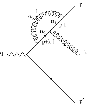
Figure B.4: Diagram representing $T_{2m}$.

We are referring, as far as the denominator structure is concerned, to a Feynman diagram of the type depicted in Fig. B.4

$$T_{2m} \equiv \int\frac{d^{d}l}{(2\pi)^{d}}\ \frac{1}{l^{2}}\ \frac{1}{(l-p)^{2}-m^{2}}\ \frac{1}{(p+k-l)^{2}-m^{2}}$$ (B.66)

$$= \frac{i}{16\pi^{2}}\ (4\pi)^{\epsilon}\ \Gamma(1+\epsilon)(-1)\int\frac{[d\alpha]}{D^{1+\epsilon}}\;,\quad\quad\quad d=4-2\epsilon\;,$$

where we have performed the usual steps, already done for the previous integrations, and where

$$D = -\left[\alpha_{1}\,\alpha_{3}\,m^{2}+\alpha_{2}\,\alpha_{3}\,(p+k)^{2}\right]+(\alpha_{1}+\alpha_{2})\,m^{2}-i\eta$$ (B.67)

$$= -\left[-(\alpha_{1}+\alpha_{2}-\alpha_{1}\,\alpha_{3})\,m^{2}+\alpha_{2}\,\alpha_{3}\,s_{1}+i\eta\right]$$

$$= -\left[-m^{2}(1-\alpha_{3})^{2}+\sigma_{1}\,\alpha_{2}\,\alpha_{3}+i\eta\right]\;.$$

Continuing the integral into the unphysical region, according to eq. (B.11), we have

$$D=-\left[M^{2}(1-\alpha_{3})^{2}+\sigma_{1}\,\alpha_{2}\,\alpha_{3}\right]\;.$$ (B.68)

The integral (B.66) becomes

$$T_{2m}=\frac{i}{16\pi^{2}}\ (4\pi)^{\epsilon}\ \Gamma(1+\epsilon)\ {\rm e}^{i\pi\epsilon}\int\frac{[d\alpha]}{\left[-D\right]^{1+\epsilon}}={\rm N}(\epsilon)\,{\rm e}^{i\pi\epsilon}\,I\;,$$ (B.69)

and, with the following change of variables

$$\begin{array}[]{l}\alpha_{1}=x(1-y)\\ \alpha_{2}=xy\\ \alpha_{3}=1-x\;,\\ \end{array}$$

with Jacobian

$$\frac{\partial(\alpha_{1}\,\alpha_{2})}{\partial(x\,y)}=x\;,$$

we get

$$I=\int_{0}^{1}dx\,dy\,\frac{x}{\left[M^{2}x^{2}+\sigma_{1}x(1-x)y\right]^{1+\epsilon}}=\int_{0}^{1}dx\,dy\,\frac{x^{-\epsilon}}{\left[M^{2}x+\sigma_{1}(1-x)y\right]^{1+\epsilon}}\;.$$ (B.70)

This integral has no soft or collinear divergences, so we can put $\epsilon=0$

$$I=\int_{0}^{1}dx\,dy\,\frac{1}{M^{2}x+\sigma_{1}(1-x)y}=\int_{0}^{1}dx\,\frac{1}{\sigma_{1}(1-x)}\log\frac{M^{2}x+\sigma_{1}(1-x)}{M^{2}x}\;.$$ (B.71)

With the change of variable $z=1-x$ we obtain

$$I = \frac{1}{\sigma_{1}}\int_{0}^{1}\frac{dz}{z}\left\{\log\left[1-\left(1-\frac{\sigma_{1}}{M^{2}}\right)z\right]-\log(1-z)\right\}$$ (B.72)

$$= \frac{1}{\sigma_{1}}\left[-\,{\rm Li}_{2}\left(1-\frac{\sigma_{1}}{M^{2}}\right)+\frac{\pi^{2}}{6}\right]\;.$$

The analytic continuation into the physical region $\left(M^{2}=-m^{2}+i\eta\right)$ is straightforward. In fact we have

$$\halign{\hbox to\displaywidth{$\hfil\displaystyle#\hfil$}\cr 0.0pt{\hfil$\displaystyle\quad 1-\frac{\sigma_{1}}{M^{2}}\longrightarrow 1+\frac{\sigma_{1}}{m^{2}}+i\eta\;,\hfill\crcr}}$$

which gives

$$T_{2m}=N(\epsilon)\,\left(m^{2}\right)^{-\epsilon}\frac{1}{\sigma_{1}}\left\{\,{\rm Li}_{2}\left(-\frac{\sigma_{1}}{m^{2}}\right)+\log\frac{\sigma_{1}}{m^{2}}\log\left(1+\frac{\sigma_{1}}{m^{2}}\right)-i\,\pi\log\left(1+\frac{\sigma_{1}}{m^{2}}\right)\right\}\;,$$ (B.73)

where we have factorized out the term $(m^{2})^{-\epsilon}$, that gives zero contribution in the limit $\epsilon\,\mbox{$\rightarrow$}\,0$.

B.6 Triangle with one massive propagator: $T_{1m}$

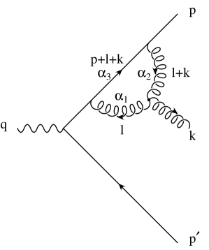
Figure B.5: Diagram representing $T_{1m}$.

We are referring, as far as the denominator structure is concerned, to a Feynman diagram of the type represented in Fig. B.5

$$T_{1m} \equiv \int\frac{d^{d}l}{(2\pi)^{d}}\ \frac{1}{l^{2}}\ \frac{1}{(l+k)^{2}}\ \frac{1}{(l+p+k)^{2}-m^{2}}$$ (B.74)

$$= \frac{i}{16\pi^{2}}\ (4\pi)^{\epsilon}\ \Gamma(1+\epsilon)(-1)\int\frac{[d\alpha]}{D^{1+\epsilon}}\;,\quad\quad\quad d=4-2\epsilon\;,$$

where, with the definition (B.11),

$$D = -\left[\alpha_{1}\,\alpha_{3}\,(p+k)^{2}+\alpha_{2}\,\alpha_{3}\,m^{2}\right]+\alpha_{3}\,m^{2}-i\eta$$ (B.75)

$$= -\left[\alpha_{1}\,\alpha_{3}\,s_{1}+\alpha_{2}\,\alpha_{3}\,m^{2}-\alpha_{3}\,m^{2}+i\eta\right]$$

$$= -\left[-m^{2}\alpha_{3}^{2}+\sigma_{1}\,\alpha_{1}\,\alpha_{3}+i\eta\right]$$

$$= -\left[M^{2}\alpha_{3}^{2}+\sigma_{1}\,\alpha_{1}\,\alpha_{3}\right]\;.$$

The integral (B.74) becomes

$$T_{1m}=\frac{i}{16\pi^{2}}\ (4\pi)^{\epsilon}\ \Gamma(1+\epsilon)\ {\rm e}^{i\pi\epsilon}\int\frac{[d\alpha]}{\left[-D\right]^{1+\epsilon}}={\rm N}(\epsilon)\,{\rm e}^{i\pi\epsilon}\,I\;,$$ (B.76)

so that, with the following change of variables

$$\begin{array}[]{l}\alpha_{1}=x(1-y)\\ \alpha_{2}=1-x\\ \alpha_{3}=xy\;,\\ \end{array}$$

and the Jacobian

$$\frac{\partial(\alpha_{1}\,\alpha_{2})}{\partial(x\,y)}=x\;,$$

we obtain

$$I=\int_{0}^{1}dx\,dy\,\frac{x}{\left[M^{2}x^{2}y^{2}+\sigma_{1}x^{2}(1-y)y\right]^{1+\epsilon}}=\int_{0}^{1}dx\,dy\,\frac{x^{-1-2\epsilon}}{\left[M^{2}y^{2}+\sigma_{1}(1-y)y\right]^{1+\epsilon}}\;.$$ (B.77)

Integrating in $x$

$$I=-\frac{1}{2\epsilon}\int_{0}^{1}dy\,\frac{y^{-1-\epsilon}}{\sigma_{1}^{1+\epsilon}\left[1+\left(\frac{M^{2}}{\sigma_{1}}-1\right)y\right]^{1+\epsilon}}\;,$$ (B.78)

and using the identity (A.8), we have

$$I = -\frac{1}{2\epsilon}\left(M^{2}\right)^{-\epsilon}\frac{1}{\sigma_{1}}\left(\frac{M^{2}}{\sigma_{1}}\right)^{2\epsilon}\int_{0}^{1}dy\,y^{-1-\epsilon}\left[1-y\left(1-\frac{\sigma_{1}}{M^{2}}\right)\right]^{2\epsilon}$$ (B.79)

$$= -\frac{1}{2\epsilon}\left(M^{2}\right)^{-\epsilon}\frac{1}{\sigma_{1}}\left(\frac{M^{2}}{\sigma_{1}}\right)^{2\epsilon}\left[-\frac{1}{\epsilon}-2\epsilon\,{\rm Li}_{2}\left(1-\frac{\sigma_{1}}{M^{2}}\right)\right]\;.$$

Expanding $\left(\frac{M^{2}}{\sigma_{1}}\right)^{2\epsilon}$ in powers of $\epsilon$

$$T_{1m}=N(\epsilon)\,{\rm e}^{i\pi\epsilon}\left(M^{2}\right)^{-\epsilon}\frac{1}{\sigma_{1}}\left[\frac{1}{2\epsilon^{2}}+\frac{1}{\epsilon}\log\frac{M^{2}}{\sigma_{1}}+\,{\rm Li}_{2}\left(1-\frac{\sigma_{1}}{M^{2}}\right)+\log^{2}\frac{M^{2}}{\sigma_{1}}\right]$$ (B.80)

and continuing analytically the solution

$$T_{1m} = N(\epsilon)\,\left(m^{2}\right)^{-\epsilon}\frac{1}{\sigma_{1}}\left\{\frac{1}{2\epsilon^{2}}+\frac{1}{\epsilon}\log\frac{m^{2}}{\sigma_{1}}+\log\frac{m^{2}}{\sigma_{1}}\log\left(1+\frac{m^{2}}{\sigma_{1}}\right)\right.$$ (B.81)

$$\left.-\,{\rm Li}_{2}\left(-\frac{\sigma_{1}}{m^{2}}\right)-\frac{5}{6}\pi^{2}+i\,\pi\left[\frac{1}{\epsilon}+\log\left(1+\frac{\sigma_{1}}{m^{2}}\right)+2\log\frac{m^{2}}{\sigma_{1}}\right]\right\}\;.\phantom{aaa}$$

B.7 First check triangle: $T_{2m}^{q-k}$

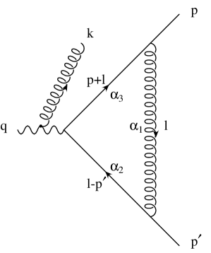
Figure B.6: Diagram representing $T_{2m}^{q-k}$.

This appendix and the following one are deserved to compute two diagrams useful for a partial check of the calculation. The denominator structure is illustrated in Fig. B.6

$$T_{2m}^{q-k} \equiv \int\frac{d^{d}l}{(2\pi)^{d}}\ \frac{1}{l^{2}}\ \frac{1}{(l-p^{\prime})^{2}-m^{2}}\ \frac{1}{(l+p)^{2}-m^{2}}$$ (B.82)

$$= \frac{i}{16\pi^{2}}\ (4\pi)^{\epsilon}\ \Gamma(1+\epsilon)(-1)\int\frac{[d\alpha]}{D^{1+\epsilon}}\;,\quad\quad\quad d=4-2\epsilon\;,$$

where

$$D = -\left[\alpha_{1}\,\alpha_{2}\,m^{2}+\alpha_{1}\,\alpha_{3}\,m^{2}+\alpha_{2}\,\alpha_{3}\,(q-k)^{2}\right]+(\alpha_{2}+\alpha_{3})\,m^{2}-i\eta$$ (B.83)

$$= -\left[-m^{2}(1-\alpha_{1})^{2}+s_{3}\,\alpha_{2}\,\alpha_{3}+i\eta\right]$$

$$= -\left[M^{2}(1-\alpha_{1})^{2}+s_{3}\,\alpha_{2}\,\alpha_{3}\right]\;.$$

The integral (B.82) becomes

$$T_{2m}^{q-k}=\frac{i}{16\pi^{2}}\ (4\pi)^{\epsilon}\ \Gamma(1+\epsilon)\ {\rm e}^{i\pi\epsilon}\int\frac{[d\alpha]}{\left[-D\right]^{1+\epsilon}}={\rm N}(\epsilon)\,{\rm e}^{i\pi\epsilon}\,I\;,$$ (B.84)

and, by changing the variables of integration,

$$\begin{array}[]{l}\alpha_{1}=1-x\\ \alpha_{2}=xz\\ \alpha_{3}=x(1-z)\;,\\ \end{array}$$

with Jacobian

$$\frac{\partial(\alpha_{1}\,\alpha_{2})}{\partial(x\,y)}=x\;,$$

we have

$$I=\int_{0}^{1}dx\,dz\,\frac{x}{\left[M^{2}x^{2}+x^{2}z(1-z)s_{3}\right]^{1+\epsilon}}=\int_{0}^{1}dx\,dz\,\frac{x^{-1-2\epsilon}}{\left[M^{2}+z(1-z)s_{3}\right]^{1+\epsilon}}\;.$$ (B.85)

Performing the $x$ integration, we obtain

$$I=-\frac{1}{2\epsilon}\left(M^{2}\right)^{-\epsilon}\int_{0}^{1}dz\frac{1}{M^{2}\left[1+z(1-z)\frac{s_{3}}{M^{2}}\right]^{1+\epsilon}}\;,$$ (B.86)

which is equal to the integral computed in eq. (3), so that we have

$$T_{2m}^{q-k} = N(\epsilon)\,{\rm e}^{i\pi\epsilon}\left(M^{2}\right)^{-\epsilon}\frac{1}{s_{3}\Delta^{\prime}}\left\{\frac{1}{\epsilon}\log\frac{-\xi_{-}}{\xi_{+}}+\log\frac{M^{2}}{s_{3}}\log\frac{-\xi_{-}}{\xi_{+}}-\frac{1}{2}\log^{2}(-\xi_{-})\right.$$ (B.87)

$$\left.{}+\frac{1}{2}\log^{2}\xi_{+}-\log\Delta^{\prime}\log\frac{-\xi_{-}}{\xi_{+}}+\,{\rm Li}_{2}\left(-\frac{\xi_{-}}{\Delta^{\prime}}\right)-\,{\rm Li}_{2}\left(\frac{\xi_{+}}{\Delta^{\prime}}\right)\right\}\;.$$

The analytic continuation of this solution, using

$$\halign{\hbox to\displaywidth{$\hfil\displaystyle#\hfil$}\cr 0.0pt{\hfil$\displaystyle\quad\frac{\xi_{+}}{\Delta^{\prime}}>1\longrightarrow\frac{\xi_{+}}{\Delta^{\prime}}-i\eta\;,\hfill\crcr}}$$

is

$$T_{2m}^{q-k} = N(\epsilon)\,\left(m^{2}\right)^{-\epsilon}\frac{1}{s_{3}\Delta^{\prime}}\left\{\frac{1}{\epsilon}\log\frac{\xi_{-}}{\xi_{+}}+\log\frac{m^{2}}{s_{3}}\log\frac{\xi_{-}}{\xi_{+}}-\frac{1}{2}\log^{2}\xi_{-}+\frac{1}{2}\log^{2}\xi_{+}\right.$$ (B.88)

$$-\log\Delta^{\prime}\log\frac{\xi_{-}}{\xi_{+}}+\,{\rm Li}_{2}\left(-\frac{\xi_{-}}{\Delta^{\prime}}\right)+\,{\rm Li}_{2}\left(\frac{\Delta^{\prime}}{\xi_{+}}\right)+\frac{1}{2}\log^{2}\frac{\xi_{+}}{\Delta^{\prime}}-\frac{5}{6}\pi^{2}$$

$$\left.+\,i\,\pi\left[\frac{1}{\epsilon}+\log\frac{m^{2}}{s_{3}}-2\log\Delta^{\prime}\right]\right\}\;.$$

B.8 Second check triangle: $T_{3m}$

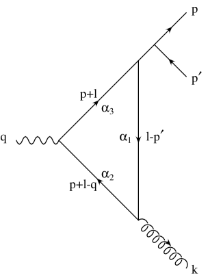
Figure B.7: Diagram representing $T_{3m}$.

This appendix (as the previous one) is deserved to calculate a diagram used for a partial check of the calculation. The denominator structure is depicted in Fig. B.7

$$T_{3m} \equiv \int\frac{d^{d}l}{(2\pi)^{d}}\ \frac{1}{(l-p^{\prime})^{2}-m^{2}}\ \frac{1}{(l+p-q)^{2}-m^{2}}\ \frac{1}{(l+p)^{2}-m^{2}}$$ (B.89)

$$= \frac{i}{16\pi^{2}}\ (4\pi)^{\epsilon}\ \Gamma(1+\epsilon)(-1)\int\frac{[d\alpha]}{D^{1+\epsilon}}\;,\quad\quad\quad d=4-2\epsilon\;,$$

where

$$D = -\left[\alpha_{1}\,\alpha_{2}\,(p+p^{\prime})^{2}+\alpha_{2}\,\alpha_{3}\,q^{2}\right]+m^{2}-i\eta$$ (B.90)

$$= -\left[-m^{2}+\alpha_{1}\,\alpha_{2}\,s_{3}+\alpha_{2}\,\alpha_{3}\,q^{2}+i\eta\right]$$

$$= -\left[M^{2}+s_{3}\,\alpha_{1}\,\alpha_{3}+q^{2}\alpha_{2}\,\alpha_{3}\right]\;.$$

The integral (B.89) becomes

$$T_{3m}=\frac{i}{16\pi^{2}}\ (4\pi)^{\epsilon}\ \Gamma(1+\epsilon)\ {\rm e}^{i\pi\epsilon}\int\frac{[d\alpha]}{\left[-D\right]^{1+\epsilon}}={\rm N}(\epsilon)\,{\rm e}^{i\pi\epsilon}\,I\;,$$ (B.91)

and, with the following change of variables,

$$\begin{array}[]{l}\alpha_{1}=xy\\ \alpha_{2}=x(1-y)\\ \alpha_{3}=1-x\;,\\ \end{array}$$

we have a Jacobian

$$\frac{\partial(\alpha_{1}\,\alpha_{2})}{\partial(x\,y)}=x\;,$$

so that

$$I=\int_{0}^{1}dx\,dy\,\frac{x}{\left[s_{3}\,x(1-x)y+q^{2}x(1-x)(1-y)+M^{2}\right]^{1+\epsilon}}\;.$$ (B.92)

This diagram has no soft or collinear divergences, and then we can put $\epsilon=0$, and we can integrate in $y$ to obtain

$$I=\frac{1}{s_{3}-q^{2}}\int_{0}^{1}dx\ \frac{1}{1-x}\log\frac{M^{2}+x(1-x)s_{3}}{M^{2}+x(1-x)q^{2}}\;.$$ (B.93)

By splitting $\log\left(a/b\right)=\log a-\log b$ and using

$$\int_{0}^{1}\frac{dx}{x}\log\left[1+x(1-x)\frac{s_{3}}{M^{2}}\right] = \int_{0}^{1}\frac{dx}{x}\log\left(1-\frac{x}{\xi_{+}}\right)+\int_{0}^{1}\frac{dx}{x}\log\left(1-\frac{x}{\xi_{-}}\right)$$

$$= -\,{\rm Li}_{2}\left(\frac{1}{\xi_{+}}\right)-\,{\rm Li}_{2}\left(\frac{1}{\xi_{-}}\right)=\frac{1}{2}\log^{2}\left(1-\frac{1}{\xi_{-}}\right)\;,$$

we have

$$T_{3m}=N(\epsilon)\,\frac{1}{2}\,\frac{1}{s_{3}-q^{2}}\left\{\log^{2}\left(1-\frac{1}{\xi_{-}}\right)-\log^{2}\left(1-\frac{1}{\lambda_{-}}\right)\right\}\;.$$ (B.94)

The analytic continuation gives

$$T_{3m} = N(\epsilon)\left(m^{2}\right)^{-\epsilon}\frac{1}{2}\,\frac{1}{s_{3}-q^{2}}\left\{\log^{2}\left(\frac{1}{\xi_{-}}-1\right)-\log^{2}\left(\frac{1}{\lambda_{-}}-1\right)\right.$$ (B.95)

$$\left.{}-2\,i\,\pi\left[\log\left(\frac{1}{\xi_{-}}-1\right)-\log\left(\frac{1}{\lambda_{-}}-1\right)\right]\right\}\;.$$

B.9 Partial check of the virtual integrals

B.9.1 Check of $B_{2m}$

A partial check of the correctness of the above formulae can be performed in the following way. We consider first a check of $B_{2m}$. To this purpose, we define $I$ as

$$I \equiv \int\frac{d^{d}l}{(2\pi)^{d}}\ \frac{1+A(l-k)^{2}+B\left[(l+p-q)^{2}-m^{2}\right]+C\left[(l+p)^{2}-m^{2}\right]}{l^{2}(l-k)^{2}\left[(l+p-q)^{2}-m^{2}\right]\left[(l+p)^{2}-m^{2}\right]}$$

$$= \int\frac{d^{d}l}{(2\pi)^{d}}\ \frac{1+B[q^{2}-2p\cdot q]+2l\cdot\left[-Ak+B(p-q)+Cp\right]+l^{2}(A+B+C)}{l^{2}(l-k)^{2}\left[(l+p-q)^{2}-m^{2}\right]\left[(l+p)^{2}-m^{2}\right]}\;.$$

If we impose that $I$ has no soft and collinear divergences, we have

$$\left\{\,\vbox{\openup 6.45831pt\halign{\strut$\displaystyle{#}$&$ \displaystyle{{}#}$\hfil\cr 1+B[q^{2}-2p\cdot q]=0\cr k\cdot\left[-Ak+B(p-q)+Cp\right]=0\;.\crcr}}\,\right.$$

The solution of this system is

$$\left\{\,\vbox{\openup 6.45831pt\halign{\strut$\displaystyle{#}$&$ \displaystyle{{}#}$\hfil\cr B=-\frac{1}{\sigma_{2}}\cr C=-\frac{1}{\sigma_{1}}\;,\crcr}}\,\right.$$

with the term $A$ undefined. We can then rewrite $I$ as

$$I = \int\frac{d^{d}l}{(2\pi)^{d}}\ \frac{2l\cdot\left[-Ak-\frac{1}{\sigma_{2}}(p-q)-\frac{1}{\sigma_{1}}p\right]+l^{2}\left(A-\frac{1}{\sigma_{1}}-\frac{1}{\sigma_{2}}\right)}{l^{2}(l-k)^{2}\left[(l+p-q)^{2}-m^{2}\right]\left[(l+p)^{2}-m^{2}\right]}$$ (B.97)

$$= B_{2m}+AT_{2m}^{{}^{\prime}q}-\frac{1}{\sigma_{2}}T_{1m}-\frac{1}{\sigma_{1}}T_{1m}^{{}^{\prime}}\;,$$

where the second line is obtained directly from eq. (B.9.1), and the primed quantities are obtained with the substitution $p\leftrightarrow p^{\prime}$, that is $\sigma_{1}\leftrightarrow\sigma_{2}$. The integral $I$ is now convergent and the cancellation of the divergent part in the right-hand side can be checked directly (both in the real part and in the absorptive one). In fact:
cancellation of the terms proportional to ${\displaystyle\mathbf{\frac{1}{\epsilon^{2}}}}$

$$\underbrace{\frac{1}{\sigma_{1}\sigma_{2}}}_{B_{2m}}-\frac{1}{\sigma_{2}}\underbrace{\frac{1}{2\sigma_{1}}}_{T_{1m}}-\frac{1}{\sigma_{1}}\underbrace{\frac{1}{2\sigma_{2}}}_{T_{1m}^{{}^{\prime}}}=0$$

cancellation of the terms proportional to ${\displaystyle\mathbf{\frac{1}{\epsilon}}}$

$$\underbrace{\frac{1}{\sigma_{1}\sigma_{2}}\left\{\log\frac{m^{2}}{\sigma_{1}}+\log\frac{m^{2}}{\sigma_{1}}+2\pi i\right\}}_{B_{2m}}-\frac{1}{\sigma_{2}}\underbrace{\frac{1}{\sigma_{1}}\left\{\log\frac{m^{2}}{\sigma_{1}}+i\pi\right\}}_{T_{1m}}-\frac{1}{\sigma_{1}}\underbrace{\frac{1}{\sigma_{2}}\left\{\log\frac{m^{2}}{\sigma_{2}}+i\pi\right\}}_{T_{1m}^{{}^{\prime}}}=0$$

cancellation of the finite terms: the finite integral $I$ of eq. (B.97) can be written as

$$I = \tilde{I}+\left(A-\frac{1}{\sigma_{1}}-\frac{1}{\sigma_{2}}\right)T_{2m}^{q}$$

$$\tilde{I} = \int\frac{d^{d}l}{(2\pi)^{d}}\ \frac{2\,l\cdot\left[-Ak-\frac{1}{\sigma_{2}}(p-q)-\frac{1}{\sigma_{1}}p\right]}{l^{2}(l-k)^{2}\left[(l+p-q)^{2}-m^{2}\right]\left[(l+p)^{2}-m^{2}\right]}\;.$$ (B.98)

In order to compute $\tilde{I}$, we introduce the Feynman parameters (see eq. (A.10)) to rewrite the denominator in the following form

$${\rm den} = \left\{\alpha_{1}l^{2}+\alpha_{4}(l-k)^{2}+\alpha_{3}\left[(l+p-q)^{2}-m^{2}\right]+\alpha_{2}\left[(l+p)^{2}-m^{2}\right]\right\}^{4}$$ (B.99)

$$= \underbrace{\left(\alpha_{1}+\alpha_{2}+\alpha_{3}+\alpha_{4}\right)}_{=1}l^{2}+2l\cdot\left[-k\,\alpha_{4}+(p-q)\,\alpha_{3}+p\,\alpha_{2}\right]+\ldots\;,$$

where the $\alpha_{i}$ are illustrated in Fig. B.1. With the following change of variable

$$l^{\prime}=l+\left[-k\,\alpha_{4}+(p-q)\,\alpha_{3}+p\,\alpha_{2}\right]\;,$$ (B.100)

we have a denominator that contains only $l^{\prime 2}$, so that $\tilde{I}$ becomes

$$\tilde{I}\! = \!\!\Gamma(4)\int\frac{d^{d}l^{\prime}}{(2\pi)^{d}}\,\int[d\alpha]\$$

$$\!\!\times\frac{2\,\Bigl{[}l^{\prime}-\left[-k\alpha_{4}+(p-q)\alpha_{3}+p\alpha_{2}\right]\Bigr{]}\cdot\left[-Ak-\frac{1}{\sigma_{2}}(p-q)-\frac{1}{\sigma_{1}}p\right]}{\left[l^{\prime 2}+\ldots\right]^{4}}$$

$$= \!\!N(\epsilon)\,(1+\epsilon)\,{\rm e}^{i\pi\epsilon}\!\!\int[d\alpha]\frac{-2\,\left[-k\alpha_{4}+(p-q)\alpha_{3}+p\,\alpha_{2}\right]\cdot\left[-Ak-\frac{1}{\sigma_{2}}(p-q)-\frac{1}{\sigma_{1}}p\right]}{\left[-m^{2}(\alpha_{2}+a_{3})^{2}+\sigma_{2}\,\alpha_{1}\,\alpha_{3}+q^{2}\alpha_{2}\,\alpha_{3}+\sigma_{1}\,\alpha_{2}\,\alpha_{4}\right]^{2}}\;,$$

where we have put $\epsilon=0$ in the integral because it is finite by construction. Expanding the dot-product we get

$$\tilde{I} = N(\epsilon)\,(1+\epsilon)\,{\rm e}^{i\pi\epsilon}\int[d\alpha]\frac{-2\left(\alpha_{3}H+\alpha_{2}K\right)}{[-(\alpha_{2}+a_{3})^{2}m^{2}+\sigma_{2}\alpha_{1}\alpha_{3}+q^{2}\alpha_{2}\alpha_{3}+\sigma_{1}\alpha_{2}\alpha_{4}]^{2}}$$ (B.101)

$$\equiv N(\epsilon)\,(1+\epsilon)\,{\rm e}^{i\pi\epsilon}(-2)\left[HI_{3}+KI_{2}\right]\;,$$

where

  $${H=\frac{\sigma_{2}}{2}A-1-m^{2}\left(\frac{1}{\sigma_{1}}+\frac{1}{\sigma_{2}}\right)+\frac{q^{2}-\sigma_{2}}{2\sigma_{1}}} {K=-\frac{\sigma_{1}}{2}A-m^{2}\left(\frac{1}{\sigma_{1}}+\frac{1}{\sigma_{2}}\right)+\frac{q^{2}-\sigma_{2}}{2\sigma_{2}}\;.}$$  

In the Euclidean region used to compute the one-loop integrals and with the change of variables of eq. (B.14), we have

$$I_{\left\{2,3\right\}}=\int_{0}^{1}dx\,dy\,dz\,\frac{(1-y)\left\{x,(1-x)\right\}}{\left[M^{2}y+\sigma_{2}z(1-x)(1-y)+q^{2}xy(1-x)+\sigma_{1}x(1-y)(1-z)\right]^{2}}\;.$$

Performing the $z$ and $y$ integration, we obtain

$$I_{\left\{2,3\right\}} = \int_{0}^{1}dx\,\left\{\frac{1}{M^{2}+q^{2}x(1-x)-\sigma_{1}x}\log\frac{M^{2}+q^{2}x(1-x)}{\sigma_{1}x}\right.$$

$$\left.-\frac{1}{M^{2}+q^{2}x(1-x)-\sigma_{2}(1-x)}\log\frac{M^{2}+q^{2}x(1-x)}{\sigma_{2}(1-x)}\right\}\frac{\left\{x,(1-x)\right\}}{\sigma_{2}(1-x)-\sigma_{1}x}\;.$$

This integral can be expressed in terms of dilogarithm and logarithm functions; nevertheless we have performed a numerical integration in order to check the identity (B.97).

B.9.2 Check of $B_{3m}$

With a reasoning similar to the previous one, we can check $B_{3m}$. We introduce the following integral

$$I \equiv \int\frac{d^{d}l}{(2\pi)^{d}}\ \frac{1+A\left[(l+p)^{2}-m^{2}\right]+B\left[(l+p-q)^{2}-m^{2}\right]+C\left[(l-p^{\prime})^{2}-m^{2}\right]}{l^{2}\left[(l+p)^{2}-m^{2}\right]\left[(l+p-q)^{2}-m^{2}\right]\left[(l-p^{\prime})^{2}-m^{2}\right]}$$

$$= \int\frac{d^{d}l}{(2\pi)^{d}}\ \frac{1+B\left[q^{2}-2p\cdot q\right]+2l\cdot\left[Ap+B(p-q)-Cp^{\prime}\right]+l^{2}(A+B+C)}{l^{2}\left[(l+p)^{2}-m^{2}\right]\left[(l+p-q)^{2}-m^{2}\right]\left[(l-p^{\prime})^{2}-m^{2}\right]}\;.$$

This integral has only soft singularities, but no collinear ones, which can be removed if we require that

$$1+B\left[q^{2}-2p\cdot q\right]=0\;,$$

that is

$$B=-\frac{1}{\sigma_{2}}\;,$$

with $A$ and $C$ undefined. We can rewrite $I$ as

$$I = \int\frac{d^{d}l}{(2\pi)^{d}}\ \frac{2\,l\cdot\left[Ap+-\frac{1}{\sigma_{2}}(p-q)-Cp^{\prime}\right]+l^{2}(A-\frac{1}{\sigma_{2}}+C)}{l^{2}\left[(l+p)^{2}-m^{2}\right]\left[(l+p-q)^{2}-m^{2}\right]\left[(l-p^{\prime})^{2}-m^{2}\right]}$$ (B.102)

$$= B_{3m}+AT_{2m}^{{}^{\prime}}-\frac{1}{\sigma_{2}}T_{2m}^{q-k}+CT_{2m}^{{}^{\prime}q}\;,$$

where the primed quantities are obtained with the substitution $p\leftrightarrow p^{\prime}$, that is $\sigma_{1}\leftrightarrow\sigma_{2}$. The integral $I$ is now convergent and the cancellation of the divergent part in the right-hand side can be checked directly (both in the real part and in the absorptive one). In fact:
cancellation of the terms proportional to ${\displaystyle\mathbf{\frac{1}{\epsilon}}}$

$$\underbrace{\frac{1}{\sigma_{2}s_{3}\Delta^{\prime}}\left(\log\frac{\xi_{-}}{\xi_{+}}+i\pi\right)}_{B_{3m}}-\frac{1}{\sigma_{2}}\underbrace{\frac{1}{s_{3}\Delta^{\prime}}\left(\log\frac{\xi_{-}}{\xi_{+}}+i\pi\right)}_{T_{2m}^{q-k}}=0$$

cancellation of the finite terms: the finite integral $I$ of eq. (B.102) can be written as

$$I = \tilde{I}+\left(A-\frac{1}{\sigma_{2}}+C\right)T_{3m}$$

$$\tilde{I} \equiv \int\frac{d^{d}l}{(2\pi)^{d}}\,\frac{2\,l\cdot\left[Ap-\frac{1}{\sigma_{2}}(p-q)-Cp^{\prime}\right]}{l^{2}\left[(l+p)^{2}-m^{2}\right]\left[(l+p-q)^{2}-m^{2}\right]\left[(l-p^{\prime})^{2}-m^{2}\right]}\;.$$ (B.103)

With the same procedure used to check $B_{2m}$ in the previous appendix, we can write

$$\tilde{I}=N(\epsilon)\,(1+\epsilon)\ {\rm e}^{i\pi\epsilon}\int[d\alpha]\frac{-2\left[\alpha_{2}p+\alpha_{3}(p-q)-\alpha_{4}p^{\prime}\right]\cdot\left[Ap-\frac{1}{\sigma_{2}}(p-q)-Cp^{\prime}\right]}{\left[-m^{2}(1-\alpha_{1})^{2}+\sigma_{2}\,\alpha_{1}\,\alpha_{3}+q^{2}\alpha_{2}\,\alpha_{3}+s_{3}\,\alpha_{2}\,\alpha_{4}\right]^{2}}\;,$$

where we have put $\epsilon=0$ in the integral because it is now finite, and the $\alpha_{i}$ are illustrated in Fig. B.2. Expanding the dot-product, we have

$$\tilde{I} = N(\epsilon)\,(1+\epsilon)\ {\rm e}^{i\pi\epsilon}\int[d\alpha]\frac{-2\left(\alpha_{2}J+\alpha_{3}L+\alpha_{4}R\right)}{\left[-m^{2}(1-\alpha_{1})^{2}+\sigma_{2}\,\alpha_{1}\,\alpha_{3}+q^{2}\alpha_{2}\,\alpha_{3}+s_{3}\,\alpha_{2}\,\alpha_{4}\right]^{2}}$$ (B.104)

$$\equiv N(\epsilon)\,(1+\epsilon)\ {\rm e}^{i\pi\epsilon}(-2)\left[JI_{2}+LI_{3}+RI_{4}\right]\;,$$

where

  $${J=\left(A-\frac{1}{\sigma_{2}}+C\right)m^{2}+\frac{1}{\sigma_{2}}\frac{q^{2}-\sigma_{2}}{2}-\frac{q^{2}-\sigma_{1}-\sigma_{2}}{2}C} {L=\left(A-\frac{1}{\sigma_{2}}+C\right)m^{2}-\frac{q^{2}-\sigma_{2}}{2}A-1+\frac{\sigma_{2}}{2}C} {R=\left(A-\frac{1}{\sigma_{2}}+C\right)m^{2}-\frac{q^{2}-\sigma_{1}-\sigma_{2}}{2}A-\frac{1}{2}\;.}$$  

In the Euclidean region used to compute the one-loop integrals and with the change of variables of eq. (B.40), we have

$$I_{\left\{2,3,4\right\}}=\int_{0}^{1}dx\,dy\,dz\,\frac{xz\left\{(1-z),yz,(1-y)z\right\}}{[M^{2}x+\sigma_{2}(1-x)yz+s_{3}x(1-y)z(1-z)+q^{2}xyz(1-z)]^{2}}\;.$$

From the identity

$$\int_{0}^{1}dx\,\frac{x}{[ax+b]^{2}}=\frac{1}{a^{2}}\left[\log\frac{a+b}{b}+\frac{b}{a+b}-1\right]\;,$$ (B.105)

we can integrate in $x$, where $a$ and $b$ are given by

  $${a=M^{2}-\sigma_{2}yz+s_{3}(1-y)z(1-z)+q^{2}yz(1-z)} {b=\sigma_{2}yz\;.}$$  

At this stage of the integration, $I_{\left\{2,3,4\right\}}$ are two-variable integrals, which can be expressed in terms of dilogarithm and logarithm functions; nevertheless we have performed a numerical integration in order to check the identity (B.102).

B.10 Self energy with one massive propagator: $S_{1m}$

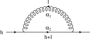
Figure B.8: Diagram representing $S_{1m}$.

We are referring, as far as the denominator structure is concerned, to a Feynman diagram of the type illustrated in Fig. B.8

$$S_{1m}\equiv\int\frac{d^{d}l}{(2\pi)^{d}}\ \frac{1}{l^{2}}\ \frac{1}{(h+l)^{2}-m^{2}}=\frac{i}{16\pi^{2}}\ (4\pi)^{\epsilon}\ \Gamma(\epsilon)\int\frac{[d\alpha]}{D^{\epsilon}}\;,\quad\quad\quad d=4-2\epsilon\;,\phantom{aaa}$$ (B.106)

where $h^{2}\geq m^{2}$ and

$$D=-\alpha_{1}\,\alpha_{2}\,h^{2}+\alpha_{2}\,m^{2}-i\eta\;.$$ (B.107)

We assume $h^{2}<0$ and, at the end, we return to the physical region according to the $i\eta$ prescription. We then define

$$H^{2}=-(h^{2}+i\eta)>0\;,$$

so that

$$D=H^{2}\alpha_{1}\,\alpha_{2}+m^{2}\alpha_{2}\;,$$ (B.108)

and, with the following change of variables,

$$\begin{array}[]{l}\alpha_{1}=1-x\\ \alpha_{2}=x\;,\\ \end{array}$$

we obtain (the Jacobian is equal to 1)

$$S_{1m} = \frac{i}{16\pi^{2}}\ (4\pi)^{\epsilon}\ \frac{\Gamma(1+\epsilon)}{\epsilon}\,\int_{0}^{1}dx\,\frac{1}{\Bigl{[}m^{2}x+H^{2}x(1-x)\Bigr{]}^{\epsilon}}$$ (B.109)

$$= N(\epsilon)\,\left(m^{2}\right)^{-\epsilon}\frac{1}{\epsilon}\int_{0}^{1}dx\,\frac{x^{-\epsilon}}{\left[1+\frac{H^{2}}{m^{2}}(1-x)\right]^{\epsilon}}\;.$$

The integral is finite, and then, expanding in $\epsilon$, we get

$$S_{1m} = N(\epsilon)\,\left(m^{2}\right)^{-\epsilon}\frac{1}{\epsilon}\left\{1-\epsilon\int_{0}^{1}dx\,\log x-\epsilon\int_{0}^{1}dx\,\log\left[1+\frac{H^{2}}{m^{2}}(1-x)\right]\right\}$$ (B.110)

$$= N(\epsilon)\,\left(m^{2}\right)^{-\epsilon}\left\{\frac{1}{\epsilon}+2-\left(1+\frac{m^{2}}{H^{2}}\right)\log\left(1+\frac{H^{2}}{m^{2}}\right)\right\}\;.$$

For $h^{2}\geq m^{2}$, we have to continue our solution according to

$$\halign{\hbox to\displaywidth{$\hfil\displaystyle#\hfil$}\cr 0.0pt{\hfil$\displaystyle\quad\log\left(1+\frac{H^{2}}{m^{2}}\right)\longrightarrow\log\left(1-\frac{h^{2}}{m^{2}}-i\eta\right)=\log\left(\frac{h^{2}}{m^{2}}-1\right)-i\pi\;,\hfill\crcr}}$$

and we obtain

$$S_{1m}=N(\epsilon)\,\left(m^{2}\right)^{-\epsilon}\left\{\frac{1}{\epsilon}+2-\left(1-\frac{m^{2}}{h^{2}}\right)\log\left(\frac{h^{2}}{m^{2}}-1\right)+i\pi\left(1-\frac{m^{2}}{h^{2}}\right)\right\}\;.$$ (B.111)

Two particular expressions are interesting: $S_{1m}$ and its derivate computed at $h^{2}=m^{2}$. The first expression is easily done

$$\left.S_{1m}\right|_{h^{2}=m^{2}}\equiv S_{1mm}=N(\epsilon)\,\left(m^{2}\right)^{-\epsilon}\left(\frac{1}{\epsilon}+2\right)\;.\\$$

For the derivate, we have to start from eq. (B.109)

$$\left.\frac{\partial S_{1m}}{\partial h^{2}}\right|_{h^{2}=m^{2}} = N(\epsilon)\,\left(m^{2}\right)^{-\epsilon}\frac{1}{\epsilon}\int_{0}^{1}dx\,\left.\frac{\epsilon\,\frac{1}{m^{2}}\,x^{-\epsilon}(1-x)}{\left[1-\frac{h^{2}}{m^{2}}(1-x)\right]^{1+\epsilon}}\right|_{h^{2}=m^{2}}$$ (B.112)

$$= N(\epsilon)\,\left(m^{2}\right)^{-\epsilon}\frac{1}{m^{2}}\int_{0}^{1}dx\,x^{-1-2\epsilon}(1-x)$$

$$= N(\epsilon)\,\left(m^{2}\right)^{-\epsilon}\frac{1}{m^{2}}\left(-\frac{1}{2\epsilon}-1\right)\;.$$

B.11 Self energy with two massive propagators: $S_{2m}$

Figure B.9: Diagram representing $S_{2m}$.

We are referring, as far as the denominator structure is concerned, to a Feynman diagram of the type represented in Fig. B.9

$$S_{2m}\equiv\int\frac{d^{d}l}{(2\pi)^{d}}\ \frac{1}{l^{2}-m^{2}}\ \frac{1}{(l-h)^{2}-m^{2}}=\frac{i}{16\pi^{2}}\ (4\pi)^{\epsilon}\ \Gamma(\epsilon)\int\frac{[d\alpha]}{D^{\epsilon}}\;,\quad\quad\quad d=4-2\epsilon\;,$$ (B.113)

where $h^{2}\geq 4m^{2}$ and

$$D=-h^{2}\alpha_{1}\,\alpha_{2}+m^{2}-i\eta\;.$$ (B.114)

Again we assume $h^{2}<0$ and define

$$H^{2}=-(h^{2}+i\eta)>0\;.$$

The Jacobian of the following change of variables is equal to 1,

$$\begin{array}[]{l}\alpha_{1}=x\\ \alpha_{2}=1-x\;,\\ \end{array}$$

so that

$$S_{2m} = \frac{i}{16\pi^{2}}\ (4\pi)^{\epsilon}\ \frac{\Gamma(1+\epsilon)}{\epsilon}\,\int_{0}^{1}dx\,\frac{1}{\left[m^{2}+H^{2}x(1-x)\right]^{\epsilon}}$$

$$= N(\epsilon)\,\left(m^{2}\right)^{-\epsilon}\frac{1}{\epsilon}\int_{0}^{1}dx\,\frac{1}{\left[1+\frac{H^{2}}{m^{2}}x(1-x)\right]^{\epsilon}}\;.$$

The integral is finite, and we can expand in $\epsilon$

$$S_{2m} = N(\epsilon)\,\left(m^{2}\right)^{-\epsilon}\frac{1}{\epsilon}\left\{1-\epsilon\int_{0}^{1}dx\,\log\left[1+\frac{H^{2}}{m^{2}}x(1-x)\right]\right\}$$ (B.116)

$$= N(\epsilon)\,\left(m^{2}\right)^{-\epsilon}\left\{\frac{1}{\epsilon}+2+\left(\tau_{+}-\tau_{-}\right)\log\frac{-\tau_{-}}{\tau_{+}}\right\}\;,$$

where we have used the fact that

$$1+\frac{H^{2}}{m^{2}}x(1-x)=\frac{H^{2}}{m^{2}}(\tau_{+}-x)(x-\tau_{-})$$

with

$$\tau_{\pm}=\frac{1}{2}\left(1\pm\sqrt{1+\frac{4m^{2}}{H^{2}}}\right)\;.$$

If we are interested in the value of $h^{2}$ such that $h^{2}\geq 4m^{2}$, we continue analytically our solution

$$\tau_{\pm}=\frac{1}{2}\left(1\pm\sqrt{1-\frac{4m^{2}}{h^{2}}}\right)\pm i\eta\;,$$ (B.117)

and we obtain

$$S_{2m}=N(\epsilon)\,\left(m^{2}\right)^{-\epsilon}\left\{\frac{1}{\epsilon}+2+\left(\tau_{+}-\tau_{-}\right)\log\frac{\tau_{-}}{\tau_{+}}+i\,\pi\left(\tau_{+}-\tau_{-}\right)\right\}\;.$$ (B.118)

Two particular cases are interesting: the one with $m=0$ and the one with $h^{2}\approx 0$. For both cases, we start from eq. (B.11). If $m=0$ we have

$$\left.S_{2m}\right|_{m=0}={\rm N}(\epsilon)\,\left(H^{2}\right)^{-\epsilon}\,\frac{1}{\epsilon}\int_{0}^{1}dx\,x^{-\epsilon}(1-x)^{-\epsilon}={\rm N}(\epsilon)\left(h^{2}\right)^{-\epsilon}{\rm e}^{i\pi\epsilon}\left(\frac{1}{\epsilon}+2\right)\;.$$ (B.119)

When $h^{2}\approx 0$, we can expand eq. (B.11) in $\epsilon$ and $h^{2}$

$$\left.S_{2m}\right|_{h^{2}\approx 0} = N(\epsilon)\,\left(m^{2}\right)^{-\epsilon}\frac{1}{\epsilon}\int_{0}^{1}dx\,\left[1-\epsilon\log\left(1-\frac{h^{2}}{m^{2}}\,x\,(1-x)\right)+{\cal O}\left(\epsilon^{2}\right)\right]$$ (B.120)

$$= N(\epsilon)\,\left(m^{2}\right)^{-\epsilon}\frac{1}{\epsilon}\int_{0}^{1}dx\,\left[1+\epsilon\left(\frac{h^{2}}{m^{2}}\,x\,(1-x)\right)+{\cal O}\left(h^{4}\right)\right]$$

$$= N(\epsilon)\,\left(m^{2}\right)^{-\epsilon}\left\{\frac{1}{\epsilon}+\frac{1}{6}\,\frac{h^{2}}{m^{2}}\right\}\;.$$

In addition

$$\left(S_{2m}\right)_{\mu}\equiv\int\frac{d^{d}l}{(2\pi)^{d}}\ \frac{l_{\mu}}{\left(l^{2}-m^{2}\right)\left[(l-h)^{2}-m^{2}\right]}=\frac{h_{\mu}}{2}\,S_{2m}\;,$$ (B.121)

that can be demonstrated by contracting both sides with $h^{\mu}$, and expanding

$$h\cdot l=-\frac{1}{2}\left\{\left[(l-h)^{2}-m^{2}\right]-\left[l^{2}-m^{2}\right]-h^{2}\right\}\;.$$ (B.122)

In the same way, we can write

$$\left(S_{2m}\right)_{\mu\nu}\equiv\int\frac{d^{d}l}{(2\pi)^{d}}\ \frac{l_{\mu}\,l_{\nu}}{\left(l^{2}-m^{2}\right)\left[(l-h)^{2}-m^{2}\right]}=A\,\frac{h_{\mu}\,h_{\nu}}{h^{2}}+B\,g_{\mu\nu}\;,$$ (B.123)

with

$$A = \frac{1}{d-1}\left[\left(\frac{d}{2}-1\right)L_{1m}+\left(\frac{d}{4}\,h^{2}-m^{2}\right)S_{2m}\right]$$

$$B = \frac{1}{d-1}\left[\frac{1}{2}\,L_{1m}+\left(m^{2}-\frac{h^{2}}{4}\right)S_{2m}\right]\;,$$ (B.124)

that can be obtained by contracting eq. (B.123) with $h^{\nu}$ and with $g^{\mu\nu}$. The expression of $L_{1m}$ is given in eq. (B.131).

B.12 Vacuum polarization with two massive propagators: $P_{2m}$

Figure B.10: Diagram representing $P_{2m}$.

This appendix and the following one are to be regarded as particular cases of Appendix B.11. Nevertheless, we summarize here the results. The structure of the denominators of this Feynman diagram is depicted in Fig. B.10

$$P_{2m}\equiv\int\frac{d^{d}l}{(2\pi)^{d}}\ \frac{1}{l^{2}-m^{2}}\ \frac{1}{(l-k)^{2}-m^{2}}=\frac{i}{16\pi^{2}}\ (4\pi)^{\epsilon}\ \Gamma(\epsilon)\int\frac{[d\alpha]}{D^{\epsilon}}\;,\quad\quad\quad d=4-2\epsilon\;,$$ (B.125)

with

$$k^{2}=0\;,\quad\quad\quad D=(\alpha_{1}+\alpha_{2})\,m^{2}-i\eta=m^{2}\;.$$ (B.126)

The result is simply given by

$$P_{2m}=\frac{i}{16\pi^{2}}\ (4\pi)^{\epsilon}\ \frac{\Gamma(1+\epsilon)}{\epsilon}\ \int_{0}^{1}d\alpha\ \frac{1}{\left(m^{2}\right)^{\epsilon}}=N(\epsilon)\,\left(m^{2}\right)^{-\epsilon}\frac{1}{\epsilon}\;,$$ (B.127)

that agrees with eq. (B.120) for $h^{2}=0$.

B.13 Vacuum polarization with no massive propagator: $P_{0m}$

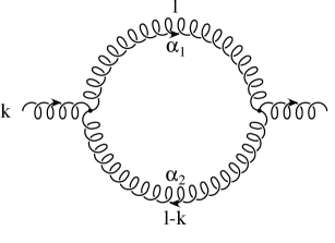
Figure B.11: Diagram representing $P_{0m}$.

We are referring, as far as the denominator structure is concerned, to a Feynman diagram of the type represented in Fig. B.11

$$P_{0m}\equiv\int\frac{d^{d}l}{(2\pi)^{d}}\ \frac{1}{l^{2}}\ \frac{1}{(l-k)^{2}}\;,\quad\quad\quad d=4-2\epsilon\;.$$ (B.128)

Since no invariant scalars are present, because $k^{2}=0$, we have

$$P_{0m}=0\;.$$ (B.129)

B.14 Massive loop: $L_{1m}$

Figure B.12: Diagram representing $L_{1m}$.

The single loop is illustrated in Fig. B.12

$$L_{1m}\equiv\int\frac{d^{d}l}{(2\pi)^{d}}\ \frac{1}{l^{2}-m^{2}}\;,\quad\quad\quad d=4-2\epsilon\;,$$ (B.130)

and can be easily integarted

$$L_{1m}=-\frac{i}{(4\pi)^{2}}\,(4\pi)^{\epsilon}\,\frac{\Gamma(-1+\epsilon)}{\left(m^{2}\right)^{-1+\epsilon}}=N(\epsilon)\,\left(m^{2}\right)^{-\epsilon}m^{2}\left(\frac{1}{\epsilon}+1\right)\;.$$ (B.131)

A particular case is the massless loop, where, again, we do not have invariants to build the solution

$$L_{0m}\equiv\int\frac{d^{d}l}{(2\pi)^{d}}\ \frac{1}{l^{2}}=0\;.$$ (B.132)

Chapter C Renormalization

C.1 Radiative corrections to external heavy-quark lines

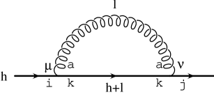
Figure C.1: Diagram representing the quark self-energy $\Sigma_{ij}(h)$.

In this appendix we describe how to treat loop corrections to external heavy-quark lines and how to compute the mass counterterm.

The one loop correction to a quark propagator reads

$$\Sigma_{ij}(h)=\int\frac{d^{d}l}{(2\pi)^{d}}\left(-ig_{s}\mu^{\epsilon}\gamma^{\nu}t_{jk}^{a}\right)\frac{i}{h\kern-5.16663pt/+l\kern-4.30554pt\hbox{/}-m}\left(-ig_{s}\mu^{\epsilon}\gamma^{\mu}t^{a}_{ki}\right)\frac{-ig_{\mu\nu}}{l^{2}}\;,$$ (C.1)

where the sum over repeated indexes is meant and $\mu$ is the mass parameter of the dimensional regularization, introduced in order to keep $g_{s}$ dimensionless. With a little algebra we have

$$\Sigma_{ij}(h) = -g_{s}^{2}\mu^{2\epsilon}C_{F}\,\delta_{ij}\int\frac{d^{d}l}{(2\pi)^{d}}\frac{\gamma^{\mu}(l\kern-4.30554pt\hbox{/}+h\kern-5.16663pt/+m)\gamma_{\mu}}{l^{2}\left[(h+l)^{2}-m^{2}\right]}$$ (C.2)

$$= -g_{s}^{2}\mu^{2\epsilon}C_{F}\,\delta_{ij}\int\frac{d^{d}l}{(2\pi)^{d}}\frac{(2-d)(h\kern-5.16663pt/+l\kern-4.30554pt\hbox{/})+d\,m}{l^{2}\left[(h+l)^{2}-m^{2}\right]}$$

$$= -g_{s}^{2}\mu^{2\epsilon}C_{F}\,\delta_{ij}\left\{\left[(2-d)h\kern-5.16663pt/+d\,m\right]\int\frac{d^{d}l}{(2\pi)^{d}}\,\frac{1}{l^{2}\left[(h+l)^{2}-m^{2}\right]}\right.$$

$$+\left.(2-d)\int\frac{d^{d}l}{(2\pi)^{d}}\,\frac{l\kern-4.30554pt\hbox{/}}{l^{2}\left[(h+l)^{2}-m^{2}\right]}\right\}\;.$$

In the last integral we can replace

$$l_{\mu}\,\mbox{$\rightarrow$}\,l\cdot h\;\frac{h_{\mu}}{h^{2}}=\frac{1}{2}\left\{\left[(h+l)^{2}-m^{2}\right]-h^{2}-l^{2}+m^{2}\right\}\,\frac{h_{\mu}}{h^{2}}\;,$$ (C.3)

and obtain

$$\Sigma_{ij}(h)\!\! = \!\!-g_{s}^{2}\mu^{2\epsilon}C_{F}\,\delta_{ij}\left\{\left[(2-d)h\kern-5.16663pt/+d\,m\right]S_{1m}+\frac{h\kern-5.16663pt/}{2h^{2}}(2-d)\!\left[\left(m^{2}-h^{2}\right)\,S_{1m}-L_{1m}\right]\!\right\}$$ (C.4)

$$= \!\!-g_{s}^{2}\mu^{2\epsilon}C_{F}\,\delta_{ij}\left\{\left[\left(-1+\epsilon-(1-\epsilon)\frac{m^{2}}{h^{2}}\right)h\kern-5.16663pt/+(4-2\epsilon)\,m\right]S_{1m}\right.$$

$${}+\left.\frac{h\kern-5.16663pt/}{h^{2}}(1-\epsilon)L_{1m}\right\}\;,$$

where we have used the definitions given by eqs. (B.106), (B.131) and (B.132) and we have specified $d=4-2\epsilon$. We are interested in the expansion of $\Sigma_{ij}(h)$ around $h\kern-5.16663pt/=m$

$$\Sigma_{ij}(h)=\left.\Sigma_{ij}(h)\right|_{h\kern-3.01389pt\hbox{/}=m}+\left(h\kern-5.16663pt/-m\right)\left.\frac{\partial\Sigma_{ij}(h)}{\partial h\kern-5.16663pt/}\right|_{h\kern-3.01389pt\hbox{/}=m}+{\cal O}\left(\left(h\kern-5.16663pt/-m\right)^{2}\right)\;.$$ (C.5)

Using the identity

$$h\kern-5.16663pt/\,h\kern-5.16663pt/=h^{2}\ \Rightarrow\ 2h\kern-5.16663pt/\,\partial h\kern-5.16663pt/=\partial h^{2}\ \Rightarrow\ \frac{\partial}{\partial h\kern-5.16663pt/}=2h\kern-5.16663pt/\frac{\partial}{\partial h^{2}}\;,$$ (C.6)

so that

$$\left.\frac{\partial\Sigma_{ij}(h)}{\partial h\kern-5.16663pt/}\right|_{h\kern-3.01389pt\hbox{/}=m}=2\,m\left.\frac{\partial\Sigma_{ij}(h)}{\partial h^{2}}\right|_{h\kern-3.01389pt\hbox{/}=m}\;,$$ (C.7)

and eqs. (B.10) and (B.112), with simple algebraic passages, we can rewrite (C.5) as

$$\Sigma_{ij}(h)\!\! = \!\!-g_{s}^{2}C_{F}\,N(\epsilon)\left(\frac{\mu^{2}}{m^{2}}\right)^{\epsilon}\!\delta_{ij}\left\{\left[\frac{3}{\epsilon}+4\right]\,m+\left(h\kern-5.16663pt/-m\right)\left[-\frac{3}{\epsilon}-4\right]\right\}+{\cal O}\left(\left(h\kern-5.16663pt/-m\right)^{2}\right)$$ (C.8)

$$\equiv \!\!\delta_{ij}\,\Bigl{[}-i\,\delta m-i\,\left(h\kern-5.16663pt/-m\right)z_{Q}\Bigr{]}+{\cal O}\left(\left(h\kern-5.16663pt/-m\right)^{2}\right)\;,$$

where

$$\delta m = -i\,g_{s}^{2}C_{F}\,N(\epsilon)\left(\frac{\mu^{2}}{m^{2}}\right)^{\epsilon}\left[\frac{3}{\epsilon}+4\right]\,m$$

$$z_{Q} = i\,g_{s}^{2}C_{F}\,N(\epsilon)\left(\frac{\mu^{2}}{m^{2}}\right)^{\epsilon}\left[\frac{3}{\epsilon}+4\right]\;.$$ (C.9)

The full quark propagator at first order reads

$$G_{Q}(h) = \frac{i\,\delta_{ij}}{h\kern-5.16663pt/-m}+\frac{i\,\delta_{ik}}{h\kern-5.16663pt/-m}\ \Sigma_{kl}(h)\ \frac{i\,\delta_{lj}}{h\kern-5.16663pt/-m}+{\cal O}\left(\alpha_{s}^{2}\right)$$ (C.10)

$$= \frac{i\,\delta_{ij}}{h\kern-5.16663pt/-m}\left(1+z_{Q}\right)+\frac{i\,\delta_{ik}}{h\kern-5.16663pt/-m}\left(-i\,\delta m\right)\frac{i\,\delta_{kj}}{h\kern-5.16663pt/-m}+\frac{{\cal O}\left(h^{2}-m^{2}\right)}{h\kern-5.16663pt/-m}\;.\phantom{aaaaa}$$

If we want that the pole of the propagator is not displaced by radiative corrections, so that $m$ corresponds to the pole mass definition, we have to add a mass counterterm to cancel the second term of the above expression. For this reason, we define the Feynman rule for the mass counterterm as the insertion, in the fermion propagator, of the vertex $-i\,m_{c}$, where

$$m_{c}=-\delta m=-g_{s}^{2}C_{F}\,N_{\epsilon}\left(\frac{\mu^{2}}{m^{2}}\right)^{\epsilon}\left[\frac{3}{\epsilon}+4\right]\,m\;,$$ (C.11)

and $N_{\epsilon}$ is defined in eq. (5.38), that is

$$N_{\epsilon}=-i\,N(\epsilon)=\frac{1}{16\pi^{2}}\left(4\pi\right)^{\epsilon}\Gamma(1+\epsilon)\;.$$

In this way, slightly off-shell, the quark propagator behaves like

$$G_{Q}(h)=\frac{i\,\delta_{ij}}{h\kern-5.16663pt/-m}\,Z_{Q}\;,$$ (C.12)

with

$$Z_{Q}=1+z_{Q}=1-g_{s}^{2}C_{F}\,N_{\epsilon}\left(\frac{\mu^{2}}{m^{2}}\right)^{\epsilon}\left[\frac{3}{\epsilon}+4\right]\;.$$ (C.13)

C.2 Radiative corrections to external gluon lines

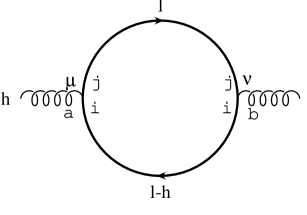
Figure C.2: Diagram representing the gluon self-energy contribution coming from a massive-quark loop.

Gluon, light-fermion and ghost self-energy corrections to external gluon lines vanish in dimensional regularization, so we need to consider only the correction coming from the heavy-flavour loop, represented in Fig. C.2. This contribution is given by

$$\Pi_{\mu\nu}^{ab}=-\int\frac{d^{d}l}{(2\pi)^{d}}\mathop{\rm Tr}\left[\left(-ig_{s}\mu^{\epsilon}\gamma_{\nu}t_{ij}^{b}\right)\frac{i}{l\kern-4.30554pt\hbox{/}-m}\left(-ig_{s}\mu^{\epsilon}\gamma_{\mu}t^{a}_{ji}\right)\frac{i}{l\kern-4.30554pt\hbox{/}-h\kern-5.16663pt/-m}\right]\;,$$ (C.14)

where the minus sign takes care of the fermion loop. With simple algebra

$$\Pi_{\mu\nu}^{ab}\!\! = \!\!-g_{s}^{2}\mu^{2\epsilon}\,T_{F}\,\delta^{ab}\int\frac{d^{d}l}{(2\pi)^{d}}\frac{\mathop{\rm Tr}\Bigl{[}\gamma_{\mu}\left(l\kern-4.30554pt\hbox{/}+m\right)\gamma_{\nu}\left[\left(l\kern-4.30554pt\hbox{/}-h\kern-5.16663pt/\right)+m\right]\Bigr{]}}{\left(l^{2}-m^{2}\right)\left[\left(l-h\right)^{2}-m^{2}\right]}$$ (C.15)

$$= \!\!4\,g_{s}^{2}\mu^{2\epsilon}\,T_{F}\,\delta^{ab}\int\frac{d^{d}l}{(2\pi)^{d}}\frac{g_{\mu\nu}\left(l^{2}-m^{2}\right)-g_{\mu\nu}\,l\cdot h-2\,l_{\mu}l_{\nu}+l_{\mu}h_{\nu}+l_{\nu}h_{\mu}}{\left(l^{2}-m^{2}\right)\left[\left(l-h\right)^{2}-m^{2}\right]}\;,\phantom{aaaa}$$

where $\mathop{\rm Tr}\left(t^{a}t^{b}\right)=T_{F}\,\delta^{ab}$, $T_{F}=1/2$. Using eqs. (B.113), (B.121) and (B.123), we can write

$$\Pi_{\mu\nu}^{ab}=4\,g_{s}^{2}\mu^{2\epsilon}\,T_{F}\,\delta^{ab}h^{2}\left[g_{\mu\nu}-\frac{h_{\mu}h_{\nu}}{h^{2}}\right]\Pi(h^{2})\;,$$ (C.16)

where

$$\Pi(h^{2})=\frac{d-2}{d-1}\,\frac{1}{h^{2}}\ L_{1m}-\frac{1}{d-1}\left[\frac{d}{2}-1+2\frac{m^{2}}{h^{2}}\right]S_{2m}\;.$$ (C.17)

In $d=4-2\epsilon$ dimensions, we get

$$\Pi_{\mu\nu}^{ab} = \frac{4}{3}\,g_{s}^{2}\mu^{2\epsilon}\,T_{F}\,\delta^{ab}h^{2}\left(g_{\mu\nu}-\frac{h_{\mu}h_{\nu}}{h^{2}}\right)\Bigg{\{}2\left(1-\frac{\epsilon}{3}\right)\frac{1}{h^{2}}\,L_{1m}$$ (C.18)

$${}-\left[1-\frac{\epsilon}{3}+2\,\frac{m^{2}}{h^{2}}\left(1+\frac{2}{3}\,\epsilon\right)\right]S_{2m}\Bigg{\}}\;.$$

We are interested in the form of the propagator for small gluon virtuality: using eqs. (B.120) and (B.131) we obtain

$$\Pi_{\mu\nu}^{ab}=-\frac{4}{3}\,{\rm N}(\epsilon)\,g_{s}^{2}\left(\frac{\mu^{2}}{m^{2}}\right)^{\epsilon}\,T_{F}\,\delta^{ab}h^{2}\left(g_{\mu\nu}-\frac{h_{\mu}h_{\nu}}{h^{2}}\right)\left(\frac{1}{\epsilon}+\frac{1}{6}\,\frac{h^{2}}{m^{2}}\right)\;.$$ (C.19)

It is worth noticing that, as previously stated, for small gluon virtuality and for the massless-quark loop, $\Pi(h^{2})$ is zero, because $L_{1m}=0$ and $S_{2m}\,\mbox{$\rightarrow$}\,P_{0m}=0$. The full gluon propagator at first order reads

$$G_{g}(h)\!\! = \!\!\frac{-i\,\delta^{ab}g_{\mu\nu}}{h^{2}}+\frac{-i\,\delta^{ac}g_{\mu}^{\alpha}}{h^{2}}\ \Pi_{\alpha\beta}^{cd}\ \frac{-i\,\delta^{db}g^{\beta}_{\nu}}{h^{2}}+{\cal O}\left(\alpha_{s}^{2}\right)$$ (C.20)

$$= \!\!\frac{-i\,\delta^{ab}g_{\mu\nu}}{h^{2}}-N_{\epsilon}T_{F}\,g_{s}^{2}\left(\frac{\mu^{2}}{m^{2}}\right)^{\epsilon}\frac{4}{3\,\epsilon}\frac{-i\,\delta^{ab}\left(g_{\mu\nu}-h_{\mu}h_{\nu}/h^{2}\right)}{h^{2}}+\frac{{\cal O}\left(h^{2}\right)}{h^{2}}\;.\phantom{aaaaa}$$

The part of the full propagator proportional to $h_{\mu}h_{\nu}$ gives no contribution, since it is contracted with a conserved current. For this reason we can write, for the slightly off-shell gluon propagator

$$G_{g}(h)=\frac{-i\,\delta^{ab}g_{\mu\nu}}{h^{2}}Z_{g}\;,$$ (C.21)

with

$$Z_{g}=1+z_{g}=1-N_{\epsilon}T_{F}\,g_{s}^{2}\left(\frac{\mu^{2}}{m^{2}}\right)^{\epsilon}\frac{4}{3\,\epsilon}\;.$$ (C.22)

C.3 Charge renormalization

We carry out the charge renormalization in the mixed scheme of Ref. [26], in which the $n_{\rm lf}$ light flavours are subtracted in the $\overline{\rm MS}$ scheme, while the heavy-flavour loop is subtracted at zero momentum.

In this scheme, the heavy flavour decouples at low energies. The prescription for charge renormalization is

$$\alpha_{s}\;\longrightarrow\;Z_{\alpha_{s}}\,\alpha_{s}\equiv Z_{\rm vertex}^{2}\,Z_{\rm quark}^{-2}\,Z_{\rm gluon}^{-1}\,\alpha_{s}$$ (C.23)

$$Z_{\alpha_{s}}=1+z_{\alpha_{s}}=1+g_{s}^{2}N_{\epsilon}\left[\left(\frac{4}{3\epsilon}T_{F}\,n_{\rm lf}-\frac{11}{3\epsilon}C_{A}\right)+\left(\frac{\mu^{2}}{m^{2}}\right)^{\epsilon}\frac{4}{3\epsilon}T_{F}\right]\;,$$ (C.24)

where $C_{A}=N_{c}=3$ for an SU(3) gauge theory.

We try to justify the $T_{F}$ structure of this expression without entering in the details of the calculation (albeit straightforward). Three renormalization constants determine the charge renormalization $Z_{\alpha_{s}}$: $Z_{\rm vertex}$, that takes account of the two Feynman diagrams describing quark-quark-gluon interaction; $Z_{\rm quark}$, which contains the contribution coming from the quark self-energy and $Z_{\rm gluon}$, that includes the effects of vacuum polarization.

The contributions proportional to $T_{F}$ come only from the gluon self-energy part that takes account of the corrections due to quark loops. In fact:

• the vertex correction contains the colour factors $C_{A}$ and $C_{F}$, and, in the $\overline{\rm MS}$ scheme, gives

  $$Z_{\rm vertex}=1-g_{s}^{2}N_{\epsilon}\frac{1}{\epsilon}\left[\left(C_{F}-\frac{1}{2}\,C_{A}\right)+\frac{3}{2}\,C_{A}\right]=1-g_{s}^{2}N_{\epsilon}\frac{1}{\epsilon}\left(C_{F}+C_{A}\right)$$ (C.25)

• the radiative corrections to quark propagator brings (see eq. (C.4))

  $$Z_{\rm quark}=1-g_{s}^{2}N_{\epsilon}\frac{1}{\epsilon}\,C_{F}$$ (C.26)

• the gluon- and ghost-loop corrections to gluon propagator contribute to the renormalization constant with

  $$Z_{\rm gluon}^{g,\,gh}=1+g_{s}^{2}N_{\epsilon}\frac{1}{\epsilon}\left(\frac{19}{12}\,C_{A}+\frac{1}{12}\,C_{A}\right)=1+g_{s}^{2}N_{\epsilon}\frac{5}{3\epsilon}\,C_{A}$$ (C.27)

• the contribution to the gluon self-energy coming from a massless fermion loop is given by (see eq. (C.18))

  $$\Pi_{\mu\nu}^{ab}=-\frac{4}{3}\,{\rm N}(\epsilon)\,g_{s}^{2}\,T_{F}\,\delta^{ab}h^{2}\left(g_{\mu\nu}-\frac{h_{\mu}h_{\nu}}{h^{2}}\right)\left(\frac{\mu^{2}}{h^{2}}\right)^{\epsilon}{\rm e}^{i\pi\epsilon}\left(\frac{1}{\epsilon}+\frac{5}{3}\right)\;,$$ (C.28)

  where we have used eq. (B.131) and the value of $S_{2m}$ given by eq. (B.119). In this way, in the $\overline{\rm MS}$ scheme, the massless loop contributes to the renormalization constant of the gluon propagator by an amount

  $$Z_{\rm gluon}^{q}=1-N_{\epsilon}\,T_{F}\,{n_{\rm lf}}\,g_{s}^{2}\frac{4}{3\epsilon}\;,$$ (C.29)

  where we have summed up the contributions of $n_{\rm lf}$ light quarks.

• if we subtract the heavy-flavour loop at zero momentum, we perform the same steps we have done to obtain the expression of $Z_{g}$ (see eq. (C.22)) and we get

  $$Z_{\rm gluon}^{Q}=Z_{g}=1-N_{\epsilon}T_{F}\,g_{s}^{2}\left(\frac{\mu^{2}}{m^{2}}\right)^{\epsilon}\frac{4}{3\epsilon}\;.$$ (C.30)

Combining eqs. (C.27), (C.29) and (C.30), we have

$$Z_{\rm gluon}=Z_{\rm gluon}^{g,\,gh}\times Z_{\rm gluon}^{q}\times Z_{\rm gluon}^{Q}=1-g_{s}^{2}N_{\epsilon}\left[\frac{4}{3\epsilon}\,T_{F}\,n_{\rm lf}-\frac{5}{3\epsilon}\,C_{A}+\left(\frac{\mu^{2}}{m^{2}}\right)^{\epsilon}\frac{4}{3\epsilon}\,T_{F}\right]\;.$$ (C.31)

From the definition (C.23) and the eqs. (C.25), (C.26) and (C.31), we obtain the expression of $Z_{\alpha_{s}}$ given in eq. (C.24).

Observe that, in this scheme, the term corresponding to the heavy-flavour loop (eq. (C.30)) compensates exactly the self-energy correction to the external gluon line coming from the heavy-flavour loop (eq. (C.22)): in fact, the final-state gluon is on the mass shell, so it is effectively renormalized at zero momentum by the heavy-quark loop, and thus decoupling applies.

Chapter D Soft and colliner amplitudes

D.1 Collinear limit for $g\,\mbox{$\rightarrow$}\,gg$ splitting

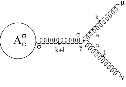
Figure D.1: Gluon splitting into a $gg$ couple.

In this appendix we derive the singular part of the square of the invariant amplitude when two collinear gluons are produced. In the collinear limit, the amplitude for the emission of two gluons in the final state can be decomposed into two parts: the first one contains the graphs where the two gluons are emitted by a single virtual one (see Fig. D.1), and the other one contains all the other graphs

$${\cal A}^{ab}=\left\{{\cal A}^{\sigma}_{c}(l+k)\,\frac{iP_{\sigma\gamma}(k+l)}{(k+l)^{2}}\,(-g_{s})\,f^{abc}\,\Gamma^{\mu\nu\gamma}(-k,-l,k+l)+{\cal R}^{\mu\nu}_{ab}\right\}\epsilon_{\mu}(k)\,\tilde{\epsilon}_{\nu}(l)\;,$$ (D.1)

where $a$ and $b$ are the colour indexes of the final gluons, $P$ is the spin projector of the gluon propagator, $g_{s}$ is the strong coupling constant, $f^{abc}$ are the structure constants of the SU(3) gauge group, $\epsilon$ and $\tilde{\epsilon}$ are the polarization vectors of the final gluons, and $\Gamma^{\mu\nu\gamma}$ is the Lorentz part of the three-gluon vertex

$$\Gamma^{\mu\nu\gamma}(-k,-l,k+l)=(-k+l)^{\gamma}g^{\mu\nu}+(-2l-k)^{\mu}g^{\nu\gamma}+(2k+l)^{\nu}g^{\mu\gamma}\;.$$ (D.2)

Only the first term of (D.1) is singular in the collinear limit. We want to stress the fact that this term is singular in the soft limit too. Therefore one has to be careful, when considering the soft and collinear limit of the square amplitude, not to include this contribution twice.

We introduce two light-like vectors $t$ and $\eta$, that, in the centre-of-mass system, have components

  $${t=\left(\left|{\bf k}+{\bf l}\,\right|,\,{\bf k}+{\bf l}\,\,\right)} {\eta=c\times\left(\frac{1}{\left|{\bf k}+{\bf l}\,\right|}\;,\,-\frac{{\bf k}+{\bf l}}{\left|{\bf k}+{\bf l}\,\right|^{2}}\right)}$$   (D.3)

and choose $c=1/4$, so that $2\,t\cdot\eta=1$. We then decompose, in the collinear limit,

$$l^{\mu}+k^{\mu}=t^{\mu}+\xi\,\eta^{\mu}\;,$$ (D.4)

where

$$\xi=(l+k)^{2}=q^{2}y\;.$$ (D.5)

We will work in the light-cone gauge, characterized by the light-like vector $\eta$, because, in this gauge, as we will see, the interference of the divergent term of (D.1) and of the finite term ${\cal R}$ does not contribute to the singular part.

In this gauge, characterized by

$$\eta^{2}=0\;,\quad\quad\quad\quad\eta\cdot\epsilon=0\;,\quad\quad\quad\quad\eta\cdot\tilde{\epsilon}=0\;,$$ (D.6)

the gluon spin projector becomes

$$P^{\sigma\gamma}(p)=-g^{\sigma\gamma}+\frac{\eta^{\sigma}p^{\gamma}+\eta^{\gamma}p^{\sigma}}{\eta\cdot p}\;,$$ (D.7)

and the transversality of gluon polarization gives

$$k\cdot\epsilon\,(k)=0\;,\quad\quad\quad\quad l\cdot\tilde{\epsilon}\,(l)=0\;.$$ (D.8)

In addition, for every momentum $p$

$$\eta_{\sigma}P^{\sigma\gamma}(p)=\eta_{\gamma}P^{\sigma\gamma}(p)=0\;.$$ (D.9)

We write $l$ and $k$ as (Sudakov decomposition)

  $${k^{\mu}=v\,t^{\mu}+\xi^{\prime}\eta^{\mu}+k_{\perp}^{\mu}} {l^{\mu}=(1-v)\,t^{\mu}+\xi^{\prime\prime}\eta^{\mu}-k_{\perp}^{\mu}\;,}$$   (D.10)

with $k_{\perp}$ such that

$$t\cdot k_{\perp}=0\;,\quad\quad\quad\quad\eta\cdot k_{\perp}=0\;.$$ (D.11)

By imposing that $k^{2}=l^{2}=0$ and that $(l+k)^{2}=q^{2}y$, we have

$$k_{\perp}^{2}=-v(1-v)\,q^{2}y\;,\quad\quad\quad\quad\xi^{\prime}=(1-v)\,q^{2}y\;,\quad\quad\quad\quad\xi^{\prime\prime}=v\,q^{2}y\;.$$ (D.12)

We can explicitly build the components of $k_{\perp}$: in fact, in the centre-of-mass system, the space-like four-vector $k_{\perp}$ can be written

$$k_{\perp}=\left(0,{\bf k}_{\perp}\right)\;,$$ (D.13)

with ${\bf k}_{\perp}$ belonging to the plane spanned by ${\bf k}$ and ${\bf l}$, and perpendicular to ${\bf k}+{\bf l}$, so that

$${\bf k}_{\perp}=a\,{\bf k}+b\,{\bf l}\;,\quad\quad\quad\quad{\bf k}_{\perp}\cdot({\bf k}+{\bf l})=0\;,\quad\quad\quad\quad k_{\perp}\cdot q=0\;.$$ (D.14)

In this way, the conditions (D.11) are fulfilled, by virtue of eqs. (D.3). It can be easily shown that eqs. (D.14) are satisfied, in the collinear limit, if

$$a\,(q\cdot k)+b\,(q\cdot l)=0\;,$$ (D.15)

so that

$$a=\frac{N}{q\cdot k}\;,\quad\quad\quad\quad b=-\frac{N}{q\cdot l}\;,$$ (D.16)

with $N$ a normalization constant, determined by the first formula of eqs. (D.12), but whose value is irrelevant to us, because we are interested in normalized quantities, like

$$\frac{k_{\perp}^{\mu}}{\sqrt{k_{\perp}^{2}}}=\frac{1}{\sqrt{-2k\cdot l}}\left[\sqrt{\frac{q\cdot l}{q\cdot k}}\;k^{\mu}-\sqrt{\frac{q\cdot k}{q\cdot l}}\;l^{\mu}\right]\;.$$ (D.17)

From eqs. (D.4) and (D.10) we obtain

$$k^{\mu} = \frac{1}{1-v}\left[v\,l^{\mu}+(1-2\,v)q^{2}y\,\eta^{\mu}+k_{\perp}^{\mu}\right]$$ (D.18)

$$l^{\mu} = \frac{1}{v}\left[(1-v)\,k^{\mu}-(1-2\,v)q^{2}y\,\eta^{\mu}-k_{\perp}^{\mu}\right]$$ (D.19)

$$l^{\mu}-k^{\mu} = (1-2\,v)\left(l^{\mu}+k^{\mu}-\xi\,\eta^{\mu}\right)+\left(\xi^{\prime\prime}-\xi^{\prime}\right)\eta^{\mu}-2\,k_{\perp}^{\mu}\;.$$ (D.20)

We are now in a position to simplify the expression of the invariant amplitude (D.1). In fact, the first term of $\Gamma^{\mu\nu\gamma}$ of eq. (D.2) becomes, with the help of eq. (D.20),

$$(-k+l)^{\gamma}P_{\sigma\gamma}(k+l)\epsilon_{\mu}(k)\,\tilde{\epsilon}_{\nu}(l) = \left[(1-2\,v)\left(l+k\right)^{\gamma}-2\,k_{\perp}^{\gamma}\right]P_{\sigma\gamma}(k+l)\epsilon_{\mu}(k)\,\tilde{\epsilon}_{\nu}(l)$$

$$= \left[(1-2\,v)2\,q^{2}y\,\eta_{\sigma}-2\,k_{\perp}^{\gamma}P_{\sigma\gamma}(k+l)\right]\epsilon_{\mu}(k)\,\tilde{\epsilon}_{\nu}(l)\;,$$

where we have used eq. (D.9) and, in the last line,

$$(k+l)^{\gamma}P_{\sigma\gamma}(k+l)=2\,q^{2}y\,\eta_{\sigma}\;.$$ (D.21)

Using eqs. (D.6), (D.8), (D.18) and (D.19) we can write the second and third term of eq. (D.2) in the following way

$$(-2l-k)^{\mu}\epsilon_{\mu}(k)\,\tilde{\epsilon}_{\nu}(l) = -2\,l^{\mu}\epsilon_{\mu}(k)\,\tilde{\epsilon}_{\nu}(l)=\frac{2}{v}\,k_{\perp}^{\mu}\epsilon_{\mu}(k)\,\tilde{\epsilon}_{\nu}(l)$$

$$(2k+l)^{\nu}\epsilon_{\mu}(k)\,\tilde{\epsilon}_{\nu}(l) = 2\,k^{\nu}\epsilon_{\mu}(k)\,\tilde{\epsilon}_{\nu}(l)=\frac{2}{1-v}\,k_{\perp}^{\nu}\epsilon_{\mu}(k)\,\tilde{\epsilon}_{\nu}(l)\;.$$ (D.22)

The amplitude (D.1) becomes

$${\cal A}^{ab}\!\! = \!\!\Biggl{\{}{\cal A}^{\sigma}_{c}(l+k)\,\frac{iP_{\sigma\gamma}(k+l)}{q^{2}y}\,(-g_{s})\,f^{abc}$$ (D.23)

$$\times\left[-2\,k_{\perp}^{\gamma}\,g^{\mu\nu}+\frac{2}{v}\,k_{\perp}^{\mu}\,g^{\nu\gamma}+\frac{2}{1-v}\,k_{\perp}^{\nu}\,g^{\mu\gamma}+{\cal O}\left(y\right)\right]+{\cal R}^{\mu\nu}_{ab}\Biggr{\}}\epsilon_{\mu}(k)\,\tilde{\epsilon}_{\nu}(l)\;.\phantom{aaaaa}$$

Observe that the first term is of order $1/\sqrt{y}$ , so that a singularity with strength $1/y$ can arise only from the square of the first term, and the interference term does not contribute. For this reason we can now substitute

$${\cal A}^{\sigma}_{c}(l+k)\ \longrightarrow\ {\cal A}^{\sigma}_{c}(t)\,\equiv\,\mbox{\rm tree-level\ amplitude}$$ (D.24)

$$P^{\sigma\gamma}(k+l)\ \longrightarrow\ P^{\sigma\gamma}(t)=-g^{\sigma\gamma}+\frac{\eta^{\sigma}t^{\gamma}+\eta^{\gamma}t^{\sigma}}{\eta\cdot t}\equiv-g_{\perp}^{\sigma\gamma}\;,$$ (D.25)

where we have neglected terms of order $k_{\perp}$, which give no contributions to the divergent part of the amplitude. Keeping only terms that contribute to the collinear singular part, we can write, with the help of eq. (D.6),

$${\cal A}^{ab}={\cal A}_{c\sigma}(t)\,\frac{g_{s}}{q^{2}y}\,if^{abc}\left[-2\,k_{\perp}^{\sigma}\,g_{\perp}^{\mu\nu}+\frac{2}{v}\,k_{\perp}^{\mu}\,g_{\perp}^{\nu\sigma}+\frac{2}{1-v}\,k_{\perp}^{\nu}\,g_{\perp}^{\mu\sigma}\right]\epsilon_{\mu}(k)\,\tilde{\epsilon}_{\nu}(l)\;.$$ (D.26)

By squaring the amplitude and summing over the colours and spins of the final gluons, we obtain, for the collinear singular part,

$${\cal M}_{\rm gg}^{\rm col} = \frac{g_{s}^{2}}{q^{2}}\,\frac{4\,C_{A}}{y}\left\{-\left[-2+\frac{1}{v}+\frac{1}{1-v}+v\,(1-v)\right]g_{\sigma\sigma^{\prime}}\right.$$ (D.27)

$$\left.{}-2\,v\,(1-v)(1-\epsilon)\left[\frac{k_{\perp\sigma}k_{\perp\sigma^{\prime}}}{k_{\perp}^{2}}-\frac{g_{\perp\sigma\sigma^{\prime}}}{2-2\,\epsilon}\right]\right\}{\cal A}_{c}^{\sigma}(t){\cal A}_{c}^{*\sigma^{\prime}}(t)\;,$$

where we have used the gauge invariance $t_{\sigma}\,{\cal A}_{c}^{\sigma}(t)=0$ to write the following identity

$${\cal A}_{c}^{\sigma}(t){\cal A}_{c}^{*\sigma^{\prime}}(t)\,g_{\perp\sigma\sigma^{\prime}}={\cal A}_{c}^{\sigma}(t){\cal A}_{c}^{*\sigma^{\prime}}(t)\,g_{\sigma\sigma^{\prime}}\;,$$

and

$$k_{\perp}^{\mu\nu}k_{\perp\mu\nu}=d-2=2-2\,\epsilon\;.$$ (D.28)

The first term of eq. (D.27) is recognized to be the Altarelli-Parisi splitting function for the gluon-gluon process, in $d=4-2\epsilon$ dimensions. The second term vanishes after azimuthal average in $4-2\epsilon$ dimensions, as can be seen from eq. (5.28).

Coming now to our problem, we can further specify the structure of ${\cal A}_{c}^{\sigma}(t){\cal A}_{c}^{*\sigma^{\prime}}(t)$. In fact, by using eq. (4.33), we can write eq. (D.27) in the following form

$${\cal M}_{\rm gg}^{\rm col} = g_{s}^{2}\,\mu^{2\epsilon}\,\frac{4\,C_{A}}{q^{2}\,y}\,\Biggl{\{}-\left[-2+\frac{1}{v}+\frac{1}{1-v}+v\,(1-v)\right]g_{\sigma\sigma^{\prime}}$$ (D.29)

$${}-2\,v\,(1-v)(1-\epsilon)\left[\frac{k_{\perp\sigma}k_{\perp\sigma^{\prime}}}{k_{\perp}^{2}}-\frac{g_{\perp\sigma\sigma^{\prime}}}{2-2\,\epsilon}\right]\Biggr{\}}\times{\cal M}_{b}^{\sigma\sigma^{\prime}}\;.$$

D.2 Collinear limit for $g\,\mbox{$\rightarrow$}\,q\bar{q}$ splitting

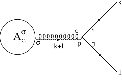
Figure D.2: Gluon splitting into a $q\bar{q}$ couple.

In this appendix, we derive the singular part of the square of the amplitude for the emission of a collinear couple of massless quark-antiquark. The invariant amplitude of the process, represented in Fig. D.2, is

$${\cal A}_{ij}={\cal A}_{c}^{\sigma}(k+l)\,\frac{iP_{\rho\sigma}(k+l)}{(k+l)^{2}}\,\bar{u}(k)\left(-ig_{s}\gamma^{\rho}t^{c}_{ij}\right)v(l)\;,$$ (D.30)

where $P$ is given by eq. (D.7) and $t^{c}$ are the generators of SU(3) gauge symmetry. By squaring this amplitude and summing over the spins and colours of the final quarks, we obtain

$${\cal M}_{\rm q\bar{q}}^{\rm col}=\frac{T_{F}\,g_{s}^{2}}{q^{4}y^{2}}{\cal A}_{c}^{\sigma}(k+l){\cal A}_{c}^{*\sigma^{\prime}}(k+l)P_{\rho\sigma}(k+l)P_{\rho^{\prime}\sigma^{\prime}}(k+l)\mathop{\rm Tr}\left(k\kern-4.30554pt\hbox{/}\gamma^{\rho}l\kern-4.30554pt\hbox{/}\gamma^{\rho^{\prime}}\right)\;,$$ (D.31)

where $t^{c}$ are normalized such that $\mathop{\rm Tr}\left(t^{a}t^{b}\right)=T_{F}\,\delta^{ab}$.

Considering now eqs. (D.10), we see that, in the collinear limit, the trace is of the order of $y$, so that the singular part can be obtained by putting $y=0$ in the rest of the numerator

$${\cal M}_{\rm q\bar{q}}^{\rm col}=\frac{T_{F}\,g_{s}^{2}}{q^{4}y^{2}}{\cal A}_{c}^{\sigma}(t){\cal A}_{c}^{*\sigma^{\prime}}(t)\,g_{\perp\rho\sigma}g_{\perp\rho^{\prime}\sigma^{\prime}}\mathop{\rm Tr}\left(k\kern-4.30554pt\hbox{/}\gamma^{\rho}l\kern-4.30554pt\hbox{/}\gamma^{\rho^{\prime}}\right)\;,$$ (D.32)

where we have used the definition of $t$ given in eq. (D.4). Evaluating the trace and keeping in the numerator only the terms proportional to $y$, we obtain

$${\cal M}_{\rm q\bar{q}}^{\rm col}=\frac{T_{F}\,g_{s}^{2}}{q^{4}y^{2}}\,4\left[-2k_{\perp\sigma}k_{\perp\sigma^{\prime}}-\frac{q^{2}y}{2}g_{\sigma\sigma^{\prime}}\right]{\cal A}_{c}^{\sigma}(t){\cal A}_{c}^{*\sigma^{\prime}}(t)\;,$$ (D.33)

that is

$${\cal M}_{\rm q\bar{q}}^{\rm col} = \frac{g_{s}^{2}}{q^{2}}\,\frac{4\,T_{F}}{y}\Biggl{\{}-\frac{1}{2-2\epsilon}\left[v^{2}+(1-v)^{2}-\epsilon\right]g_{\sigma\sigma^{\prime}}$$ (D.34)

$${}+2\,v\,(1-v)\left[\frac{k_{\perp\sigma}k_{\perp\sigma^{\prime}}}{k_{\perp}^{2}}-\frac{g_{\perp\sigma\sigma^{\prime}}}{2-2\epsilon}\right]\Biggr{\}}{\cal A}_{c}^{\sigma}(t){\cal A}_{c}^{*\sigma^{\prime}}(t)\;.$$

Here again we can recognize the Altarelli-Parisi kernel for $g\,\mbox{$\rightarrow$}\,q\bar{q}$ splitting.

As previously done for eq. (D.27) , we can specify this formula to the problem we are studying: with the help of eq. (4.33), we can write

$${\cal M}_{\rm q\bar{q}}^{\rm col} = g_{s}^{2}\,\mu^{2\epsilon}\,\frac{4\,T_{F}}{q^{2}\,y}\,\Bigg{\{}-\frac{1}{2-2\epsilon}\left[v^{2}+(1-v)^{2}-\epsilon\right]g_{\sigma\sigma^{\prime}}$$ (D.35)

$${}+2\,v\,(1-v)\left[\frac{k_{\perp\sigma}k_{\perp\sigma^{\prime}}}{k_{\perp}^{2}}-\frac{g_{\perp\sigma\sigma^{\prime}}}{2-2\epsilon}\right]\Biggr{\}}\times{\cal M}_{b}^{\sigma\sigma^{\prime}}\;.$$

D.3 Soft limit for the invariant amplitude $Q\overline{Q}gg$

In this appendix we derive the divergent part of the invariant amplitude for the process

$$Z/\gamma(q)\;\mbox{$\rightarrow$}\;Q(p)+\overline{Q}(p^{\prime})+g(k)+g(l)\;,$$ (D.36)

in the limit when the momentum $l$ of the gluon is soft. A soft singularity appears only if the soft gluon is emitted from one of the external legs.

If the emitting external particle is the gluon, the amplitude of the process, in the Feynman gauge, is

$${\cal A}^{ab{\rm(g)}}_{ij}={\cal A}^{c\sigma}_{ij}(l+k)\,\frac{-i}{(k+l)^{2}}\,(-g_{s})\,f^{abc}\,\Gamma^{\mu\nu}_{\sigma}(-k,-l,k+l)\,\epsilon_{\mu}(k)\,\tilde{\epsilon}_{\nu}(l)\;,$$ (D.37)

where we have added to eq. (D.1) the colour indexes $i,j$ of the produced quarks.
As $l$ goes to zero, this term develops a singularity: in fact, by using the gauge condition $k^{\sigma}\,{\cal A}_{c\sigma}^{ij}(k)=0$ and eq. (D.8), we can write this amplitude as

$${\cal A}^{ab{\rm(g)}}_{ij}=g_{s}f^{abc}\,\frac{k^{\nu}}{k\cdot l}\,{\cal A}^{c\sigma}_{ij}(k)\,\epsilon_{\sigma}(k)\,\tilde{\epsilon}_{\nu}(l)+\mbox{\rm non-singular terms.}$$ (D.38)

Similarly, if we consider the emission of a soft gluon of colour index $b$ from an external quark leg with momentum $p$ and colour index $i$, that is

$$Q_{n}(p+l)\,\mbox{$\rightarrow$}\,Q_{i}(p)+g_{b}(l)\;,$$

we can write the invariant amplitude

$${\cal A}_{ij}^{ab{\rm(Q)}}=\bar{u}(p)(-ig_{s}\gamma^{\nu}t^{b}_{in})\,\frac{i}{p\kern-4.30554pt\hbox{/}+l\kern-4.30554pt\hbox{/}-m}\,\tilde{\cal{A}}_{nj}^{a\mu}(p+l)\,\epsilon_{\mu}(k)\,\tilde{\epsilon}_{\nu}(l)\;,$$ (D.39)

where $\tilde{\cal{A}}$ refers to the rest of the process from which the quark external line takes origin. In the limit of $l$ going to zero, we can rewrite this amplitude as

$${\cal A}_{ij}^{ab{\rm(Q)}}=g_{s}\,\frac{p^{\nu}}{p\cdot l}\,t^{b}_{in}\,{\cal{A}}_{nj}^{a\mu}(p)\,\epsilon_{\mu}(k)\,\tilde{\epsilon}_{\nu}(l)+\mbox{\rm non-singular terms,}$$ (D.40)

where we have defined

$${\cal{A}}_{nj}^{a\mu}(p)=\bar{u}(p)\tilde{\cal{A}}_{nj}^{a\mu}(p)\;.$$ (D.41)

In the same way, we can obtain the limit of the amplitude for the soft emission from an antiquark with momentum $p^{\prime}$ and colour index $j$

$${\cal A}_{ij}^{ab{\rm(\overline{Q})}}=-g_{s}\,\frac{p^{\prime\nu}}{p^{\prime}\cdot l}\,{\cal{A}}_{in}^{a\mu}(p^{\prime})\,t^{b}_{nj}\,\epsilon_{\mu}(k)\,\tilde{\epsilon}_{\nu}(l)+\mbox{\rm non-singular terms.}$$ (D.42)

Considering that ${\cal{A}}_{ij}^{c\sigma}$ of eq. (D.38) can be written as

$${\cal{A}}_{ij}^{c\sigma}=t^{c}_{ij}{\cal{A}}^{\sigma}\;,$$ (D.43)

where ${\cal{A}}^{\sigma}$ does not contain any colour element, and the similar ones for eqs. (D.40) and (D.42), we can sum the three amplitudes to obtain

$${\cal A}_{ij}^{ab}=g_{s}\left\{if^{abc}\,\frac{k^{\nu}}{k\cdot l}\,t^{c}_{ij}+\frac{p^{\nu}}{p\cdot l}\,t^{b}_{in}\,t^{a}_{nj}-\frac{p^{\prime\nu}}{p^{\prime}\cdot l}\,t^{a}_{in}\,t^{b}_{nj}\right\}{\cal{A}}^{\mu}\,\epsilon_{\mu}(k)\,\tilde{\epsilon}_{\nu}(l)\;,$$ (D.44)

where we have disregarded the non-singular terms.

By squaring the amplitude and summing over the spins and colours of the final gluons and quarks, we have

$${\cal M}_{\rm gg}^{\rm soft}(l)\!\! = \!\!g_{s}^{2}\,\mu^{2\epsilon}\left\{-C_{A}\left[\frac{p\cdot k}{(p\cdot l)\,(k\cdot l)}+\frac{p^{\prime}\cdot k}{(p^{\prime}\cdot l)\,(k\cdot l)}\right]\right.$$ (D.45)

$$\!\!\left.{}-2\left(C_{F}-\frac{C_{A}}{2}\right)\frac{p\cdot p^{\prime}}{(p\cdot l)\,(p^{\prime}\cdot l)}+C_{F}\left[\frac{m^{2}}{(p\cdot l)^{2}}+\frac{m^{2}}{(p^{\prime}\cdot l)^{2}}\right]\right\}\times{\cal M}^{\sigma}_{\sigma}\phantom{aaaaa}$$

where we have made use of eq. (4.33).

The same result applies in the case of $k$ soft, once the interchange $l\leftrightarrow k$ is made.

Chapter E List of integrals for the four-jet singular soft contributions

In this appendix, we summarize the values of the integrals required to isolate the singular terms of the four-jet cross section, in the soft-gluon limit. The form of the integrals we are going to compute is the following

$$I=\frac{1}{N_{\phi}}\int_{0}^{\pi}d\phi\,(\sin\phi)^{-2\epsilon}\int_{0}^{x}dy\int_{0}^{1}dv\,f(y,v,\phi)\;.$$ (E.1)

We fix our attention to the $y$ and $v$ variables and we split the integration range into two triangles

$$\int_{0}^{x}dy\int_{0}^{1}dv\,f(y,v,\phi)=\int_{0}^{x}dy\int_{0}^{y/x}dv\,f(y,v,\phi)+\int_{0}^{x}dy\int_{y/x}^{1}dv\,f(y,v,\phi)\;.$$ (E.2)

We perform the following change of variables: $v=y\,t$ in the first integral and $v=y/t$ in the last one. In this way, we obtain

$$\int_{0}^{x}dy\int_{0}^{1}dv\,f(y,v,\phi) = \int_{0}^{x}dy\int_{0}^{1/x}dt\,y\,f(y,y\,t,\phi)+\int_{0}^{x}dy\int_{y}^{x}dt\,\frac{y}{t^{2}}\,f\left(y,\frac{y}{t},\phi\right)$$

$$= \int_{0}^{1/x}dt\int_{0}^{x}dy\,y\,f(y,y\,t,\phi)+\int_{0}^{x}dt\int_{0}^{t}dy\,\frac{y}{t^{2}}\,f\left(y,\frac{y}{t},\phi\right)\;,$$

where, in the second line, we have exchanged the order of integration.

In this way we succeed in writing $I$ as the sum of two contributions

$$I \equiv I^{(1)}+I^{(2)}$$ (E.3)

$$I^{(1)} \equiv \frac{1}{N_{\phi}}\int_{0}^{\pi}d\phi\,(\sin\phi)^{-2\epsilon}\int_{0}^{1/x}dt\int_{0}^{x}dy\,y\,f(y,y\,t,\phi)$$ (E.4)

$$I^{(2)} \equiv \frac{1}{N_{\phi}}\int_{0}^{\pi}d\phi\,(\sin\phi)^{-2\epsilon}\int_{0}^{x}dt\int_{0}^{t}dy\,\frac{y}{t^{2}}\,f\left(y,\frac{y}{t},\phi\right)\;.$$ (E.5)

${\mathbf{I}_{1}}$-type integrals

The first type of integrals to compute is

$$I_{1}(x,h)\equiv\frac{1}{N_{\phi}}\int_{0}^{\pi}d\phi\,(\sin\phi)^{-2\epsilon}\int_{0}^{x}dy\int_{0}^{1}dv\,[v(1-v)]^{-\epsilon}y^{-\epsilon}\frac{1}{y\,[y+h\,v]}\;.$$ (E.6)

As $f(y,v,\phi)=1/y\,[y+h\,v]$ is $\phi$-independent, the $\phi$ integration is straightforward and, according to eq. (E.4), we have

$$I_{1}^{(1)} = \int_{0}^{1/x}dt\int_{0}^{x}dy\,y^{-1-2\epsilon}\left(1-y\,t\right)^{-\epsilon}\frac{t^{-\epsilon}}{1+h\,t}$$ (E.7)

$$= \int_{0}^{1/x}dt\,\frac{t^{-\epsilon}}{1+h\,t}\int_{0}^{x}dy\,y^{-1-2\epsilon}\left[1-\epsilon\log(1-y\,t)+{\cal O}\left(\epsilon^{2}\right)\right]$$

$$= \int_{0}^{1/x}dt\,\frac{t^{-\epsilon}}{1+h\,t}\left[-\frac{1}{2\epsilon}x^{-2\epsilon}-\epsilon\int_{0}^{x}dy\,y^{-2\,\epsilon}\frac{\log(1-y\,t)}{y}+{\cal O}\left(\epsilon^{2}\right)\right]\;.\phantom{aaaaa}$$

The integral in $y$ is finite so it gives contribution of order $\epsilon$ that can be neglected. In this way we have

$$I_{1}^{(1)} = -\frac{1}{2\,\epsilon}\,x^{-2\epsilon}\int_{0}^{1/x}dt\left(1-\epsilon\log t+{\cal O}\left(\epsilon^{2}\right)\right)\frac{1}{1+h\,t}$$ (E.8)

$$= -\frac{1}{2\,h\,\epsilon}\,x^{-2\epsilon}\left\{\log\left(1+\frac{h}{x}\right)+\epsilon\left[\log x\log\left(1+\frac{h}{x}\right)-\,{\rm Li}_{2}\left(-\frac{h}{x}\right)\right]\right\}\;,\phantom{aaaa}$$

where terms of order $\epsilon$ are not computed. The integral of eq. (E.5) gives rise to

$$I_{1}^{(2)} = \int_{0}^{x}dt\int_{0}^{t}dy\,y^{-1-2\epsilon}\left(1-\frac{y}{t}\right)^{-\epsilon}\frac{t^{-1+\epsilon}}{t+h}$$ (E.9)

$$= \int_{0}^{x}dt\,\frac{t^{-1+\epsilon}}{t+h}\int_{0}^{t}dy\,y^{-1-2\epsilon}\left[1-\epsilon\log\left(1-\frac{y}{t}\right)+{\cal O}\left(\epsilon^{2}\right)\right]$$

$$= I_{1a}^{(2)}+I_{1b}^{(2)}\;,$$

where, for simplicity, we have separated out the integration into two terms. Performing the $y$ integration in $I_{1a}^{(2)}$, we get

$$I_{1a}^{(2)} = -\frac{1}{2\,\epsilon}\int_{0}^{x}dt\,\frac{t^{-1-\epsilon}}{t+h}=-\frac{1}{2\,h\,\epsilon}\int_{0}^{x}dt\,\left(\frac{1}{t}-\frac{1}{t+h}\right)t^{-\epsilon}$$ (E.10)

$$= -\frac{1}{2\,h\,\epsilon}\left\{-\frac{1}{\epsilon}x^{-\epsilon}-\int_{0}^{x}dt\,\frac{1-\epsilon\log t+{\cal O}\left(\epsilon^{2}\right)}{t+h}\right\}$$

$$= -\frac{1}{2\,h\,\epsilon}\left\{-\frac{1}{\epsilon}x^{-\epsilon}-\log\left(1+\frac{x}{h}\right)+\epsilon\left[\log x\log\left((1+\frac{x}{h}\right)+\,{\rm Li}_{2}\left(-\frac{x}{h}\right)\right]\right\}\phantom{aaaaa}$$

where we have neglected terms of order $\epsilon$. To compute $I_{1b}^{(2)}$, we perform the change of variable $z=y/t$ to obtain

$$I_{1b}^{(2)} = -\epsilon\int_{0}^{x}dt\,\frac{t^{-1-\epsilon}}{t+h}\int_{0}^{1}dz\,\frac{\log(1-z)}{z^{1+2\epsilon}}=\epsilon\,\frac{\pi^{2}}{6}\frac{1}{h}\left[-\frac{1}{\epsilon}x^{-\epsilon}+{\cal O}\left(1\right)\right]\;.$$ (E.11)

Collecting all terms together, according to eqs. (E.3), (E.8)–(E.11), we have

$$I_{1}(x,h)=\frac{1}{2\,h}\left\{\frac{1}{\epsilon^{2}}-\frac{1}{\epsilon}\log h-\log^{2}\frac{x}{h}+\frac{1}{2}\log^{2}h-\frac{\pi^{2}}{2}-2\,{\rm Li}_{2}\left(-\frac{x}{h}\right)\right\}+{\cal O}\left(\epsilon\right)\;.$$ (E.12)

${\mathbf{I}_{2}}$-type integrals

The second type of integrals has the following expression

$$I_{2}(x,h)\equiv\frac{1}{N_{\phi}}\int_{0}^{\pi}d\phi\,(\sin\phi)^{-2\epsilon}\int_{0}^{x}dy\int_{0}^{1}dv\,[v(1-v)]^{-\epsilon}y^{-\epsilon}\frac{1}{[y+av]^{2}}\;.$$ (E.13)

Here again, the $\phi$ integration is straightforward, and we have, according to eq. (E.4),

$$I_{2}^{(1)} = \int_{0}^{1/x}dt\int_{0}^{x}dy\,y^{-1-2\epsilon}\left(1-y\,t\right)^{-\epsilon}\frac{t^{-\epsilon}}{\left(1+h\,t\right)^{2}}$$ (E.14)

$$= \int_{0}^{1/x}dt\,\frac{t^{-\epsilon}}{\left(1+h\,t\right)^{2}}\int_{0}^{x}dy\,y^{-1-2\epsilon}\left[1-\epsilon\log(1-y\,t)+{\cal O}\left(\epsilon^{2}\right)\right]$$

$$= -\frac{1}{2\,\epsilon}\,x^{-2\epsilon}\int_{0}^{1/x}dt\,\left(1-\epsilon\log t\right)\frac{1}{\left(1+h\,t\right)^{2}}+{\cal O}\left(\epsilon\right)$$

$$= -\frac{1}{2\,h\,\epsilon}\,x^{-2\epsilon}\left\{1-\frac{x}{x+h}+\epsilon\left[\log\left(1+\frac{h}{x}\right)+\frac{h}{x+h}\log x\right]\right\}+{\cal O}\left(\epsilon\right)\;.\phantom{aaa}$$

From eq. (E.5) we obtain

$$I_{2}^{(2)} = \int_{0}^{x}dt\int_{0}^{t}dy\,y^{-1-2\epsilon}\left(1-\frac{y}{t}\right)^{-\epsilon}\frac{t^{\epsilon}}{\left(t+h\right)^{2}}$$ (E.15)

$$= \int_{0}^{x}dt\,\frac{t^{\epsilon}}{\left(t+h\right)^{2}}\int_{0}^{t}dy\,y^{-1-2\epsilon}\left[1-\epsilon\log\left(1-\frac{y}{t}\right)+{\cal O}\left(\epsilon^{2}\right)\right]$$

$$= -\frac{1}{2\,\epsilon}\int_{0}^{x}dt\,\frac{t^{-\epsilon}}{\left(t+h\right)^{2}}=-\frac{1}{2\,\epsilon}\int_{0}^{x}dt\,\left(1-\epsilon\log t+{\cal O}\left(\epsilon^{2}\right)\right)\frac{1}{\left(t+h\right)^{2}}$$

$$= -\frac{1}{2\,h\,\epsilon}\left\{\frac{x}{x+h}-\epsilon\left[\log\frac{h}{x+h}+\frac{x}{x+h}\log x\right]\right\}+{\cal O}\left(\epsilon\right)\;.\phantom{aaa}$$

Adding together these two contributions, we have

$$I_{2}(x,h)=I_{2}^{(1)}+I_{2}^{(2)}=\frac{1}{2\,h}\left\{-\frac{1}{\epsilon}-2\log\left(1+\frac{h}{x}\right)+\log h\right\}+{\cal O}\left(\epsilon\right)\;.$$ (E.16)

${\mathbf{I}_{3}}$-type integrals

The last type of integrals has the following form

$$I_{3}\equiv\frac{1}{N_{\phi}}\int_{0}^{\pi}d\phi\,(\sin\phi)^{-2\epsilon}I_{3}(x)\;,$$ (E.17)

where

$$I_{3}(x)\equiv\int_{0}^{x}dy\int_{0}^{1}dv\,[v(1-v)]^{-\epsilon}y^{-\epsilon}\frac{1}{y+h\,v}\,\frac{1}{y-c\cos\phi\sqrt{y}\sqrt{v}+g\,v}\;.$$ (E.18)

According to eq. (E.4) and  (E.5), we have

$$I_{3}^{(1)}(x) = \int_{0}^{1/x}dt\int_{0}^{x}dy\,y^{-1-2\epsilon}\left(1-y\,t\right)^{-\epsilon}\frac{t^{-\epsilon}}{(1+h\,t)\left(1-c\cos\phi\sqrt{t}+g\,t\right)}$$ (E.19)

$$= -\frac{1}{2\,\epsilon}\,x^{-2\epsilon}\int_{0}^{1/x}dt\frac{t^{-\epsilon}}{(1+h\,t)\left(1-c\cos\phi\sqrt{t}+g\,t\right)}+{\cal O}\left(\epsilon\right)$$

$$= -\frac{1}{2\,\epsilon}\left(1-2\epsilon\log x\right)\int_{0}^{1/x}dt\frac{1-\epsilon\log t}{(1+h\,t)\left(1-c\cos\phi\sqrt{t}+g\,t\right)}+{\cal O}\left(\epsilon\right)$$

$$= -\frac{1}{2\,\epsilon}\int_{0}^{1/x}dt\frac{1}{(1+h\,t)\left(1-c\cos\phi\sqrt{t}+g\,t\right)}$$

$$+\int_{0}^{1/x}dt\frac{\frac{1}{2}\log t+\log x}{(1+h\,t)\left(1-c\cos\phi\sqrt{t}+g\,t\right)}+{\cal O}\left(\epsilon\right)$$

$$I_{3}^{(2)}(x) = \int_{0}^{x}dt\int_{0}^{t}dy\,y^{-1-2\epsilon}\left(1-\frac{y}{t}\right)^{-\epsilon}\frac{t^{\epsilon}}{(t+h)\left(t-c\cos\phi\sqrt{t}+g\right)}$$ (E.20)

$$= -\frac{1}{2\,\epsilon}\int_{0}^{x}dt\frac{t^{-\epsilon}}{(t+h)\left(t-c\cos\phi\sqrt{t}+g\right)}+{\cal O}\left(\epsilon\right)$$

$$= -\frac{1}{2\,\epsilon}\int_{0}^{x}dt\frac{1-\epsilon\log t}{(t+h)\left(t-c\cos\phi\sqrt{t}+g\right)}+{\cal O}\left(\epsilon\right)$$

$$= -\frac{1}{2\,\epsilon}\int_{0}^{x}dt\frac{1}{(t+h)\left(t-c\cos\phi\sqrt{t}+g\right)}$$

$$+\int_{0}^{x}dt\frac{\frac{1}{2}\log t}{(t+h)\left(t-c\cos\phi\sqrt{t}+g\right)}+{\cal O}\left(\epsilon\right)\;.$$

From eqs. (E.17) and (E.18) we have

$$I_{3} = \frac{1}{N_{\phi}}\int_{0}^{\pi}d\phi\,(\sin\phi)^{-2\epsilon}\left[I_{3}^{(1)}(x)+I_{3}^{(2)}(x)\right]$$ (E.21)

$$= \frac{1}{N_{\phi}}\int_{0}^{\pi}d\phi\,\left[1-2\epsilon\log\left(\sin\phi\right)\right]\left[I_{3}^{(1)}(x)+I_{3}^{(2)}(x)\right]$$

$$= \frac{1}{N_{\phi}}\left\{-\frac{1}{2\,\epsilon}\,I_{\epsilon}+\frac{1}{2}\left[I_{3a}+I_{3b}\right]+I_{\phi}+{\cal O}\left(\epsilon\right)\right\}\;,$$

with

$$I_{\epsilon} = \int_{0}^{\infty}dt\,\int_{0}^{\pi}d\phi\,\frac{1}{\left(1+h\,t\right)\left(1-c\cos\phi\sqrt{t}+g\,t\right)}$$ (E.22)

$$I_{3a} = \int_{0}^{\frac{1}{x}}dt\,\int_{0}^{\pi}d\phi\,\frac{2\log x+\log t}{\left(1+h\,t\right)\left(1-c\cos\phi\sqrt{t}+g\,t\right)}$$ (E.23)

$$I_{3b} = \int_{0}^{x}dt\,\int_{0}^{\pi}d\phi\,\frac{\log t}{\left(h+t\right)\left(t-c\cos\phi\sqrt{t}+g\right)}$$ (E.24)

$$I_{\phi} = \int_{0}^{\infty}dt\,\int_{0}^{\pi}d\phi\,\frac{\log\left(\sin\phi\right)}{\left(1+h\,t\right)\left(1-c\cos\phi\sqrt{t}+g\,t\right)}\;.$$ (E.25)

We can now integrate in $\phi$ the first three expressions, using the identity

$$\int_{0}^{\pi}d\phi\,\frac{1}{a-b\cos\phi}=\frac{\pi}{\sqrt{a^{2}-b^{2}}}\;,$$

and in $t$ the last one, to obtain

$$I_{\epsilon} = \int_{0}^{\infty}dt\,\frac{1}{\left(1+h\,t\right)}\frac{\pi}{\sqrt{\left(1+g\,t\right)^{2}-c^{2}t}}$$ (E.26)

$$= \frac{\pi}{\sqrt{(g-h)^{2}+c^{2}h}}\ \log\frac{h\left(c^{2}-2g+2h+2\sqrt{(g-h)^{2}+c^{2}h}\right)}{h^{2}-\left(g-\sqrt{(g-h)^{2}+c^{2}h}\right)^{2}}$$

$$I_{3a} = \int_{0}^{\frac{1}{x}}dt\,\frac{2\log x+\log t}{\left(1+h\,t\right)}\frac{\pi}{\sqrt{\left(1+g\,t\right)^{2}-c^{2}t}}$$ (E.27)

$$I_{3b} = \int_{0}^{x}dt\,\frac{\log t}{\left(h+t\right)}\frac{\pi}{\sqrt{\left(t+g\right)^{2}-c^{2}t}}$$ (E.28)

$$I_{\phi} = \int_{0}^{\frac{\pi}{2}}d\phi\,\log\left(\sin\phi\right)\,\frac{2}{(g-h)^{2}+h\left(c\cos\phi\right)^{2}}$$ (E.29)

$${}\times\left\{\frac{2\,c\,(g+h)\cos\phi}{\sqrt{4g-c^{2}\cos^{2}\phi}}\ \arctan\frac{c\cos\phi}{\sqrt{4g-c^{2}\cos^{2}\phi}}+(g-h)\log\frac{g}{h}\right\}$$

$$= \int_{0}^{1}dt\,\frac{\log\sqrt{1-t^{2}}}{\sqrt{1-t^{2}}}\,\frac{2}{(g-h)^{2}+h\,c^{2}\,t^{2}}$$

$${}\times\left\{\frac{2\,c\,(g+h)\,t}{\sqrt{4g-c^{2}\,t^{2}}}\ \arctan\frac{c\,t}{\sqrt{4g-c^{2}\,t^{2}}}+(g-h)\log\frac{g}{h}\right\}\;,$$

where we have used the symmetry of the integral $I_{\phi}$ around the point $\pi/2$ and made the change of variable $t=\cos\phi$.

We are now in a position of further reduce the expression of $I_{\epsilon}$, to account for the actual values of the parameters: in fact, with the help of eqs. (5.15)–(5.17), (B.6) and (B.49), we have

$$I_{\epsilon}=\frac{\pi}{K}\,\frac{\left(1+\Delta^{\prime 2}\right)\left(1-\Delta^{\prime 2}\right)}{4\Delta^{\prime}}\left(1-x_{g}\right)\log\left(\frac{\xi_{+}}{\xi_{-}}\right)^{2}\;.$$ (E.30)

Ringrazio innanzi tutto il Prof. Paolo Nason, per la costante e fondamentale presenza durante il mio dottorato e per gli utili suggerimenti che mi ha dato nello svolgimento di questo calcolo. Un grazie va anche al Prof. Stefano Catani, per l’attenta lettura di questa tesi. Infine, vorrei ringraziare i miei genitori ed i miei amici di sempre, per essermi stati accanto in questi ultimi anni.

Bibliography

- [1]
- [2] R.K. Ellis, D.A. Ross and A.E. Terrano, Nucl. Phys. B178 (1981) 421.
- [3] J.A.M. Vermaseren, K.J.F. Gaemers and S.J. Oldham, Nucl. Phys. B187 (1981) 301.
- [4] K. Fabricius, G. Kramer, G. Schierholz and I. Schmitt, Z. Phys. C11 (1981) 315.
- [5] P. Nason and C. Oleari, Phys. Lett. B387 (1996) 623, hep-ph/9607347.
- [6] P. Nason and C. Oleari, Phys. Lett. B407 (1997) 57, hep-ph/9705295.
-
[7]
G. Rodrigo, Nucl. Phys. Proc. Suppl. 54A (1997) 60,
hep-ph/9609213;
G. Rodrigo, Ph. D. Thesis, Univ. of València, 1996, hep-ph/9703359;
G. Rodrigo, A. Santamaria and M. Bilenkii, Phys. Rev. Lett. 79 (1997) 193, hep-ph/9703358. - [8] M. Bilenkii, G. Rodrigo and A. Santamaria, Nucl. Phys. B439 (1995) 505.
- [9] W. Bernreuther, A. Brandenburg and P. Uwer, Phys. Rev. Lett. 79 (1997) 189, hep-ph/9703305.
- [10] A. Brandenburg and P. Uwer, preprint PITHA-97-29, hep-ph/9708350.
- [11] Z. Kunszt and P. Nason, “QCD”, in “Z Physics at LEP 1”, eds. G. Altarelli, R. Kleiss and C. Verzegnassi (Report CERN 89-08, Geneva, 1989).
- [12] A. Ballestrero, E. Maina and S. Moretti, Phys. Lett. B294 (1992) 425; Nucl. Phys. B415 (1994) 265.
- [13] L. Magnea and E. Maina, Phys. Lett. B385 (1996) 395, hep-ph/9604385.
- [14] K. Hagiwara, T. Kuruma and Y. Yamada, Nucl. Phys. B358 (1991) 80.
- [15] P. Nason and B.R. Webber, Nucl. Phys. B421 (1994) 473.
- [16] Particle Data Group, R.M. Barnett et al., Phys. Rev. D54 (1996) 1.
- [17] P. Nason and B.R. Webber, Phys. Lett. B395 (1997) 355, hep-ph/9612353.
- [18] B. Mele and P. Nason, Nucl. Phys. B361 (1991) 626.
- [19] R. Harlander and M. Steinhauser, hep-ph/9710413.
- [20] G. Altarelli and G. Parisi, Nucl. Phys. B126 (1977) 298.
- [21] G. Curci, W. Furmanski and R. Petronzio, Nucl. Phys. B175 (1980) 27.
- [22] E.G. Floratos, R. Lacaze and C. Kounnas, Nucl. Phys. B192 (1981) 417; Phys. Lett. B98 (1981) 89.
-
[23]
J. Kalinowski, K. Konishi, P.N. Scharbach and T.R. Taylor,
Nucl. Phys. B181 (1981) 253;
J. Kalinowski, K. Konishi and T.R. Taylor, Nucl. Phys. B181 (1981) 221. -
[24]
B.A. Kniehl, G. Kramer and M. Spira, Z. Phys. C76 (1997) 689,
hep-ph/9610267 version;
J. Binnewies, B.A. Kniehl and G. Kramer, Z. Phys. C76 (1997) 677,
hep-ph/9702408. - [25] W. Furmanski and R. Petronzio, Phys. Lett. 97B (1980) 437.
- [26] J. Collins, F. Wilczek and A. Zee, Phys. Rev. D18 (1978) 242.
- [27] F. Bloch and A. Nordsiek, Phys. Rev. 52 (1937) 54.
-
[28]
T. Kinoshita, J. Math. Phys. 3 (1962) 650,
T. D. Lee and M. Nauenberg, Phys. Rev. B133 (1964) 1549. - [29] L.J. Reinders, H. Rubinstein and S. Yazaki, Phys. Rep. 127 (1985) 1.
- [30] P. Nason, S. Dawson and R. K. Ellis, Nucl. Phys. B327 (1989) 49.
- [31] P. Nason and C. Oleari, preprint CERN-TH/97-209, hep-ph/9709358, to appear in Phys. Lett.
- [32] P. Nason and B.W. Webber, “QCD”, in “Physics at LEP2”, eds. G. Altarelli, T. Sjöstrand and F. Zwirner (Report CERN96-01, Geneva 1996).
- [33] P. Nason and C. Oleari, preprint CERN-TH/97-219, hep-ph/9709360, to appear in Nucl. Phys. B.