[

On Random Bubble Lattices

Abstract

We study random bubble lattices which can be produced by processes such as first order phase transitions, and derive characteristics that are important for understanding the percolation of distinct varieties of bubbles. The results are relevant to the formation of topological defects as they show that infinite domain walls and strings will be produced during appropriate first order transitions, and that the most suitable regular lattice to study defect formation in three dimensions is a face centered cubic lattice. Another application of our work is to the distribution of voids in the large-scale structure of the universe. We argue that the present universe is more akin to a system undergoing a first-order phase transition than to one that is crystallizing, as is implicit in the Voronoi foam description. Based on the picture of a bubbly universe, we predict a mean coordination number for the voids of 13.4. The mean coordination number may also be used as a tool to distinguish between different scenarios for structure formation.

]

The formation of topological defects has mostly been studied by numerical techniques on a regular lattice [1, 2, 3]; yet it is known that the numerical results for the statistical properties of topological defects depend on the lattice that is chosen for performing the simulations [4]. Our primary objective here is to consider defect formation during first order phase transitions in the continuum (also see [5, 6]) and to determine if infinite domain walls and strings will be produced. The results we obtain, however, are of wider applicability, since they apply to any process which leads to a random lattice. An example is the growth of universal large-scale structure, which leads to an observed distribution of voids in galaxy surveys.

First-order phase transitions proceed by the nucleation of bubbles of the low temperature phase in a background of the high temperature phase. The bubbles then grow, collide, and coalesce, eventually filling space with the low temperature phase. In a variety of circumstances, the low temperature phase is not unique. Here we will first consider the case where there are two low temperature phases, which we call plus ($+$) and minus ($-$). The interface between two spatial regions containing different phases is called a “domain wall”. We will be interested in determining if the $+$ and $-$ phases percolate (i.e. form infinite clusters) after the phase transition. Given that the probability of a bubble being in the plus phase is $p$, there exists a critical probability $p_{c}$ such that the + phase percolates only if $p>p_{c}$. Our goal is to determine $p_{c}$. If $p_{c}$ is found to be less than 0.5, then a range of $p$ exists for which both the $+$ and $-$ phases will percolate and, in this case, infinite domain walls will be formed [7]. We will also consider the formation of strings on the bubble lattice following the algorithm described in Ref. [1]. Here we will find that strings percolate on the bubble lattice and that there is an infinite string component to the network that is somewhat larger than that found in Ref. [1].

Let us begin by studying the structure of the random bubble lattice that is produced during a first order phase transition and later discussing percolation on this lattice. We write the bubble nucleation rate per unit volume as $\Gamma$, and we assume that the bubble walls expand at constant speed $v$. From these quantities we can define a length scale $\xi$ and a time scale $\tau$ by:

$$\xi=\biggr{(}{v\over\Gamma}\biggr{)}^{1/4}~{},\ \ \tau={1\over{(v^{3}\Gamma)^{1/4}}}~{},$$ (1)

where the exponents have been shown for bubbles in three dimensions. By rescaling all lengths (such as bubble radii) and all times by $\xi$ and $\tau$ respectively, the dependence of the problem on $\Gamma$ and $v$ is eliminated. Therefore dimensionful quantities such as the number density of bubbles of a given size can be rescaled to a universal distribution, and dimensionless quantities, such as the the critical percolation probability, will be independent of $\Gamma$ and $v$.

The scaling argument given above relies on the absence of any other length or time scales in the problem. Potentially such a scale is provided by $R_{0}$, the size of bubbles at nucleation, and our assumption is that $R_{0}<<\xi$. Also, note that we have taken all bubbles to expand at the same velocity $v$. This is justified if the low temperature phases within the bubbles are degenerate. If this degeneracy is lifted, different bubbles can expand at different velocities and this may result in lattices with varying properties. We are primarily interested in the exactly degenerate case which is relevant to the formation of topological defects.

In a computer simulation, there are two other scales that enter. These are the size of the simulation and the time over which the process is studied. If the size of the simulation is very large compared to $\xi$, the length scale is effectively infinite and does not play a role in the properties of the bubble lattice. Also, we are only interested in the bubble statistics once the bubbles fill the simulation volume and the phase transition is complete. At this stage, the properties of the bubble lattice are fixed and further evolution does not play a role. Hence, if we observe the lattice at any time greater than the phase transition completion time, the observation time will not enter the properties of the bubble lattice. We have verified numerically that quantities such as the size distribution of bubbles are universal. Hence we can simulate the random bubble lattice for any convenient choice of parameters.

We have simulated the nucleation and growth of bubbles leading to the completion of the phase transition following the scheme described in Ref. [5]. There are two ways to view this scheme. The first is a dynamic view where, as time proceeds, the number of nucleation sites are chosen from a Poisson distribution, bubbles keep growing and colliding until they fill space. The second equivalent viewpoint is static and more convenient for simulations. A certain number of spheres whose centers and radii are drawn from uniform distributions are placed in the simulation box. This corresponds to a snapshot of the bubble distribution. If the number of spheres that are laid down is large, they will fill space and the snapshot would be at a time after the phase transition has completed.

It is worth comparing the present model with currently existing models of froth. The main distinguishing feature is that the bubbles continue to grow even after they collide. This is in sharp distinction with the models used in crystal growth such as the Voronoi and the Johnson-Mehl models. In these models, crystals nucleate randomly inside a volume, grow and then, once they meet a neighboring crystal, stop growing in the direction of that neighbor. (In the Voronoi model, all crystals are nucleated at one instant while in the Johnson-Mehl model, they can nucleate at different times.) This difference between the phase transition model and the Voronoi type models is significant and the resulting lattices have different properties. Another model considered in the literature is called a “Laguerre froth”. Here the snapshot of the domains corresponds to a horizontal slice of a mountain range in which each mountain is a paraboloid. The circles of intersection of the plane and the paraboloids define the Laguerre froth [8]. In terms of bubbles, this means that the bubble walls move with a velocity that is proportional to $\sqrt{t-t_{0}}$ where $t-t_{0}$ is the time elapsed since nucleation. Such a model in two dimensions was studied by numerical methods in Ref. [9]. If the paraboloids are replaced by cones, the model comes closer to the present one. Such a model has not been analyzed previously in any number of dimensions.

A feature of our model of the first order phase transition is that bubbles cannot nucleate within already existing bubbles. This is appropriate to the case where the phases existing within bubbles are degenerate or nearly degenerate. However, in cases where a variety of non-degenerate bubbles can exist (for example, if the system has metastable vacuua), this assumption may have to be relaxed [10].

We construct the three dimensional (dual) bubble lattice by connecting the centers of bubbles that have collided (Fig. 1). The bubble lattice is almost fully triangulated though some violations of triangulation can occur. For example, if a tiny bubble gets surrounded by two large bubbles, the center of the tiny bubble will only be connected to the centers of the two surrounding bubbles and this can lead to plaquettes on the lattice that are not triangular. The characteristics of this bubble lattice hold the key to the percolation of phases and the formation of topological defects. In particular, the average number of vertices to which any vertex is connected is expected to play a crucial role. This number is called the “mean coordination number” of the lattice, and we now determine this quantity analytically.

First we consider the two dimensional case. We denote the number of points in the lattice by $P$, the number of edges by $E$ and the number of faces by $F$. Then the Euler-Poincaré formula [11] tells us

$$\chi=P-E+F$$ (2)

where, $\chi$ is the Euler character of the lattice and is related to the number of holes in the lattice (genus). In our case, the lattice covers a plane which we can compactify in some way, say by imposing periodic boundary conditions. Then $\chi$ is the genus of the compact two dimensional surface. For us it will only be important that $\chi=O(1)$. Next, if ${\bar{z}}$ is the (average) coordination number, we can see that

$$E={{\bar{z}}\over 2}P~{},$$

since, a given point is connected to ${\bar{z}}$ other points but each edge is bounded by two points. Also,

$$F={2\over 3}E~{},$$

since each line separates 2 faces but then each face is bounded by 3 lines. Now, using (2) gives

$$1-{{\bar{z}}\over 2}+{{\bar{z}}\over 3}={\chi\over P}\simeq 0~{},$$

since $P$ is assumed to be very large. Therefore, in two dimensions, ${\bar{z}}=6$, a result that first appeared in the botanical literature [12, 8].

In three dimensions the analysis to evaluate ${\bar{z}}$ is somewhat more complicated. The Euler-Poincaré formula now says

$$\chi=P-E+F-V~{},$$ (3)

where $V$ is the number of volumes in the lattice. Now, in addition to the usual coordination number ${\bar{z}}$, we also need to define a “mean face coordination number” ${\bar{y}}$ which counts the average number of faces sharing a common edge. In terms of ${\bar{y}}$ and ${\bar{z}}$, the relations between the various quantities for a triangulated three dimensional lattice are:

$$E={{\bar{z}}\over 2}P~{},\ \ F={{\bar{y}}\over 3}E~{},\ \ V={2\over 4}F~{},$$ (4)

where the first equation is as in two dimensions, the second equation follows from the definition of ${\bar{y}}$ and the fact that the lattice is triangulated, and the last relation follows because a face separates two volumes and a volume is bounded by four faces that form a tetrahedron. Inserting these relations in (3) leads to:

$${\bar{z}}={{12}\over{6-{\bar{y}}}}~{},$$ (5)

where, as before, we assume that $P$ is very large and ignore the $\chi/P$ term. Note that the relation between ${\bar{y}}$ and ${\bar{z}}$ is purely topological and will hold for any triangulated lattice.

FIG. 1.: A portion of the three dimensional dual bubble lattice.

We now want to estimate ${\bar{y}}$. For this we work in a “mean field” approximation where we assume that the edge lengths are fixed. We consider two vertices $A$ and $B$ separated by a unit distance. Now we wish to find the number of points that can be connected to both $A$ and $B$, subject to the constraint that connected points are at unit distance from each other. This will give the (average) number of faces that share the edge from $A$ to $B$ and hence will be the face coordination number ${\bar{y}}$. Let us choose $A$ to be at the center of a sphere of unit radius and $B$ to be at the North pole. Then the additional points $P_{1}$,…,$P_{y}$, have to lie on the circle at latitude 60 degrees to satisfy the distance constraint. Then one finds that the azimuthal angular separation of two sequential points $P_{i}$ and $P_{i+1}$ is 70.5 degrees. Therefore

$${\bar{y}}={{360}\over{70.5}}=5.1,$$ (6)

which then leads to [13]

$${\bar{z}}=13.4~{}.$$ (7)

It is worth noting the ingredients that have entered into the analytic estimate of ${\bar{z}}$. The relation (5) is a topological statement about the lattice, but the estimate for ${\bar{y}}$ is geometric, depending on the assumption that the edges have fixed length. In principle, the edge lengths can fluctuate but our estimate for ${\bar{y}}$ will still be valid if the fluctuations average out.

In Fig. 2 we show the distribution of coordination number in our three dimensional simulations. The average coordination number is found to be ${\bar{z}}=13.34\pm 0.05$ and agrees quite closely with the mean field result. For comparison, Voronoi foam has ${\bar{z}}=15.54$ and the Johnson-Mehl model has ${\bar{z}}>13.28$ [14]. The reason why ${\bar{z}}$ is larger in the Voronoi model is that, in this model, the cells stop growing on collision in the direction of the collision, thus leading to anisotropic growth. It can be shown that anisotropy of the cells leads to a higher value of ${\bar{z}}$ [8].

FIG. 2.: The coordination number relative frequency distribution for the three dimensional dual bubble lattice.

The mean value of $z$ is not a good characteristic of the distribution of $z$ since the distribution is skewed (the modal value of $z$ is 7) and it is of interest to characterize the entire distribution of $z$. In the literature on domain physics, attempts to derive the distribution of coordination number are often based on maximizing the “entropy” of the lattice subject to the constraints in the system. The expression used for the entropy is the one proposed by Shannon [15, 16]. On employing this procedure, one finds an exponential fall-off of the distribution. The distribution shown in Fig. 2 also has an exponential fall-off:

$$f(z)\sim\exp[-0.25z]\ ,\ \ z\gtrsim 20\ .$$ (8)

We now turn to the formation of defects on the bubble lattice. We put a + phase on a bubble with probability $p$ and a $-$ phase with probability $1-p$. We then find the size distribution of + clusters and calculate the moments of the cluster distribution function after removing the largest cluster from the distribution [17]. That is, we calculate:

$$S_{l}(p)=\sum_{s\neq s_{max}}s^{l}n_{s}(p)$$ (9)

for $l=0,1,2,...$, where the sum is over cluster sizes ($s$) but does not include the largest cluster size, and $n_{s}(p)$ is the number of clusters of size $s$ divided by the total number of bubbles. In Fig. 3 we show the first three moments as a function of $p$, where the turning point in $S_{2}$ marks the onset of percolation. To understand this, first consider the behavior of the second moment for small $p$. As we increase $p$, there are fewer + clusters (as seen from the $S_{0}$ graph) probably due to mergers, but the merged cluster sizes are bigger (as seen from the $S_{1}$ graph). Since the second moment places greater weight on the size of the cluster than on the number density as compared to the lower moments, it grows for small $p$. For large $p$, however, as we increase $p$ further, the additional + clusters join the largest cluster of +’s and are not counted in the second moment. In fact, some of the smaller clusters also merge with the largest cluster and get removed from the sum in (9). This causes the second moment to decrease at large $p$. Hence, the second moment has a turning point and the location of this turning point at $p_{c}$ marks the onset of percolation. In three dimensions we find $p_{c}=0.17\pm 0.01$ (from Fig. 3), which is well under 0.5, while in two dimensions we find $p_{c}=0.50\pm 0.01$ which is consistent with 0.50. (The two dimensional version of Fig. 3 may be found in [7].)

It is interesting to compare the critical probabilities we have found with lattice based results for site percolation where the regular lattice has a coordination number close to that of the random bubble lattice. In two dimensions a triangular lattice has ${\bar{z}}=6$ and $p_{c}=0.5$. In three dimensions, a face centered cubic lattice has ${\bar{z}}=12$ and $p_{c}=0.198$ [17]. These values of the critical probabilities are fairly close to our numerical results. Hence it seems that that most suitable regular lattice for studying first order phase transitions in two dimensions is a triangular lattice and in three dimensions is a face centered cubic lattice.

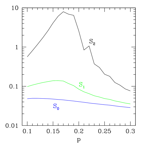
FIG. 3.: The zeroth, first and second moments of the cluster distribution function versus the probability $p$ in three dimensions.

The rather low value of $p_{c}$ in three dimensions means that domain walls formed between degenerate vacua ($p=0.5$) will percolate and almost all of the wall energy will be in one infinite wall. Furthermore, even if the vacua are not degenerate, i.e. there is bias in the system, infinite domain walls can still be produced. If the properties of the bubble lattice are insensitive to small biases, infinite domain walls would be produced for $p\gtrsim 0.17$. However, it is likely that the bubble lattice will depend on the bias in three ways. First, the nucleation rate of bubbles of the metastable vacuum will be suppressed compared to that of the true vacuum. Secondly, the velocity with which bubbles of the two phases grow can be different. Thirdly, bubbles of the true vacuum may nucleate within the metastable vacuum. In addition to these factors, bubbles may not retain their spherical shape while expanding due to instabilities in their growth. The effect of these factors on the percolation probability will be model dependent. For example, the bubble velocities will depend on the ambient plasma, and the nucleation rates on the action of the instantons between the different vacuua. The inclusion of all these effects is beyond the scope of the paper. Even so, a precise estimate of the percolation probability in certain particle physics models will be extremely useful for studying cosmological scenarios such as described in Ref. [18].

We have also investigated the formation of topological strings on the random bubble lattice following the algorithm described in Ref. [1]. We find that about 85% of the strings in the simulation are infinite. This number should be compared with earlier static simulations of string formation which yield a slightly lower fraction ($\lesssim 80\%$). All these algorithms neglect phase equilibration processes when domains of different phases collide and may be justified if the time scale $\tau$ is short compared to the typical time required for phase equilibration. In the case of domain walls, phase equilibration in two colliding bubbles can only occur by the motion of the phase separating wall across the volume of one of the bubbles. In this case, the neglect of phase equilibration is justified if the domain wall velocity is much smaller than the bubble wall velocity.

Finally, our analysis of the bubble lattice has an application to the large-scale structure of the universe. Astronomical surveys show a universe filled with vast empty regions (voids) that are outlined by walls of galaxies. If we place vertices at the centers of the voids and then connect the vertices belonging to neighboring voids, we will get a lattice much like those we have been considering in the context of first order phase transitions. Since the relation (5) is purely topological, it will also hold for the dual void lattice. Further, working in the mean field approximation for the sizes of the voids, our estimate for ${\bar{y}}$ in (6) holds. Therefore we predict that a void should have 13.4 neighboring voids on average. This prediction will be modified if there is spatial curvature in the universe, or if there are correlations between the locations of void centers and their sizes. (For example, if large voids are preferentially surrounded by small voids.) The curvature modification is, however, proportional to $\chi^{2}$ where $\chi\lesssim 10^{-2}$ is the void size divided by the spatial curvature radius, and hence is negligible for cosmology.

The modification in the void coordination number due to other cosmological factors such as cosmic expansion needs to be investigated further but a significant effect may be turned around to provide a probe of large-scale structure formation. Indeed, the distribution of coordination number (corresponding to Fig. 2) may turn out to be a valuable tool in characterizing the large-scale structure. For example, structure formation scenarios based on topological defects are likely to yield different results. In the specific case of the cosmic string scenario [19, 20], voids form on either side of a string wake and filaments form where two string wakes intersect, and so four (and not three) voids will neighbor a filament. This will lead to a void lattice that is not triangulated which will result in a lower mean coordination number. Note that the difficulty associated with defining the boundary of a void does not enter the distribution of coordination number because the number of neighbors of a given void is insensitive to the precise location of the boundaries of the voids.

The large-scale structure has often been compared to a Voronoi foam [21]. However, the phase transition model appears to be more suitable since two cells of the Voronoi foam stop growing in the direction of their collision, whereas this is not the behavior expected of large-scale voids. When two voids collide, they are better modelled as if they continue to grow as in the case of bubbles in a phase transition. Galaxies may be assumed to form in the space between bubbles which will be sheetlike while the bubbles have not collided. Upon collision, the sheetlike distribution of galaxies will get punctured. The mutual collision of three voids will yield filamentary structure and that of four voids will produce point-like structure. From these considerations, the growth of voids is more like the growth of bubbles than of crystals for which the Voronoi and Johnson-Mehl models are applicable, and the universe is more like a system currently undergoing a first-order phase transition than like one that is crystallizing. One can also consider refinements of the phase transition model that would make it yet more like the evolution of large-scale structure. For example, the growth rate of voids will be time dependent, though they would nucleate at the same epoch. Also, one could include processes in which a small void gets subsumed by a large void. We do not consider these details further in this paper.

In conclusion, we have shown that the bubble distribution resulting from a first order phase transition has a universal character and has a coordination number that we have determined analytically. The analysis shows that a triangular lattice in two dimensions and a face centered cubic lattice in three dimensions are the regular lattices that come closest to the bubble lattice. The study of percolation on the bubble lattice also supports this finding and we have found the critical percolation probability for the bubble lattice in both two and three dimensions. The result shows that infinite domain walls and strings will be produced in three dimensions. Finally we have applied our results to the void lattice in the large-scale structure of the universe and, based on some general assumptions, predict an average of 13.4 neighbors to a void.

Acknowledgments

We are grateful to Nick Rivier for his crucial input and to Harsh Mathur for extensive discussions throughout the course of this work. Comments by Christopher Thompson are gratefully acknowledged. This research was supported by the DoE.

REFERENCES

- [1] T. Vachaspati and A. Vilenkin, Phys. Rev. D30, 2036 (1984).
- [2] J. Robinson and A. Yates, Phys. Rev. D54, 5211 (1996).
- [3] R. J. Scherrer and A. Vilenkin, Phys. Rev. D56, 647 (1997); also hep-ph/9709498.
- [4] R. J. Scherrer and J. Frieman, Phys. Rev. D33, 3556 (1986).
- [5] J. Borrill, T. W. B. Kibble, T. Vachaspati and A. Vilenkin, Phys. Rev. D52, 1934 (1995).
- [6] J. Borrill, Phys. Rev. Lett. 76, 3255 (1996).
- [7] T. Vachaspati, ICTP 1997 Summer School Lectures on Cosmology, hep-ph/9710292 (1997).
- [8] This proof was provided to us by N. Rivier (private communication). For a review see the contribution by N. Rivier in “Disorder and Granular Media”, eds. D. Bideau and A. Hansen (North-Holland, 1993).
- [9] H. Telley, Ph. D. Thesis, EPFL, Lausanne, 1989 (unpublished).
- [10] M. Gleiser, A. F. Heckeler and E. W. Kolb, Phys. Lett. B405, 121 (1997).
- [11] C. Nash and S. Sen, “Topology and Geometry for Physicists”, Academic Press, London (1983).
- [12] F. T. Lewis, Anat. Record 38, 341 (1928); ibid. 50, 235 (1931).
- [13] H. S. M. Coxeter, Ill. J. Math. 2, 746 (1958); J. A. Dodds, J. Coll. Interf. Sci. 77, 317 (1980); N. Rivier, J. Physique Coll. 43, C9-91 (1982).
- [14] J. L. Meijring, Philips Res. Rep. 8, 270 (1953).
- [15] C. E. Shannon, Bell Systems Technical Journal 27, 379 (1948); reprinted in C. E. Shannon and W. Weaver, “The Mathematical Theory of Communication”, (University of Illinois Press, 1949).
- [16] N. Rivier, Phil. Mag. B52, 795 (1985).
- [17] D. Stauffer, Phys. Rep. 54, 1 (1979).
- [18] G. Dvali, H. Liu and T. Vachaspati, Phys. Rev. Lett. 80, 2281 (1998).
- [19] T. Vachaspati, Phys. Rev. Lett. 57, 1655 (1986).
- [20] T. Hara and S. Miyoshi, Prog. Theor. Phys. 81, 1187 (1989); ibid. 84, 867 (1990). In these papers the authors make the speculative though interesting point that the Coma cluster appears to be at the intersection of three sheets in the large-scale structure distribution, as might feasibly happen in the cosmic string scenario.
- [21] V. Icke and R. van de Weygaert, Astron. and Astrophys. 184, 16 (1987); R. van de Weygaert, Ph. D. thesis, Univ. Leiden (1991).