Probing the Standard Model of Particle Interactions

F. David and R. Gupta

Chapter 0 Large N QCD

1 Introduction

Quantum chromodynamics, the theory of the strong interactions, is a non-Abelian gauge theory based on the gauge group $SU(3)$. It was first pointed out by ’t Hooft [1, 2] that many features of QCD can be understood by studying a gauge theory based on the gauge group $SU(N)$ in the limit $N\rightarrow\infty$. One might think that letting $N\rightarrow\infty$ would make the analysis more complicated because of the larger gauge group and consequent increase in the number of dynamical degrees of freedom. One might also think that $SU(N)$ gauge theory has very little to do with QCD because $N=\infty$ is not close to $N=3$. However, we will soon see that $SU(N)$ gauge theory simplifies in the $N\rightarrow\infty$ limit, that the true expansion parameter is $1/N$, not $N$, and that the $1/N$ expansion is equivalent to a semiclassical expansion for an effective theory of color singlet mesons and baryons. Results for QCD can be obtained from the $N\rightarrow\infty$ limit by expanding in $1/N=1/3$, and are in good agreement with experiment.

To decide whether $1/N$ is a small expansion parameter for QCD requires further analysis. In QED, as Witten has remarked, the coupling constant $e=\sqrt{4\pi\alpha}=0.30$, which is not very different from $1/3$. Anyone who has actually computed radiative corrections in QED knows that the true expansion parameter is not $e$, but is closer to $\alpha/4\pi\approx 10^{-3}$, which is much smaller than $e$. By the end of these lectures you will see several examples which show that the expansion parameter for QCD is $1/N=1/3$. While not as small as the QED expansion parameter $\alpha/4\pi$, $1/N$ is still a useful expansion parameter for QCD. $1/N$ corrections are comparable in size to flavor $SU(3)$ breaking corrections due to the strange quark mass, and expanding in flavor $SU(3)$ breaking is well-known to be an extremely useful expansion in QCD. Furthermore, we will find many examples where the $1/N$ term vanishes, so that the first correction is of order $1/N^{2}$. In such cases, one can make predictions at the 10% level. This is a level of computational accuracy in low-energy hadronic physics that is difficult to match using other techniques.

In these lectures, I will concentrate on the large $N$ expansion for QCD, and in particular, on trying to obtain QCD results that can be compared with experimental data. Sections 2–3 and sections 6, 5–1 of these lectures are based on the treatments by Coleman [3], and Witten [4, 5], respectively. Large $N$ expansions have also been used to study other field theories, such as the $O(N)$ model, $CP^{N}$ model, etc. They provide insight into quantum field theory dynamics, and have many applications in high energy physics and statistical mechanics. They have been extensively used in recent years to study matrix models. These topics have been discussed in previous Les Houches summer schools, and will not be repeated here. A good reference on large $N$ methods is the compilation by Brezin and Wadia [6].

2 The Gross-Neveu Model

The Gross-Neveu model [7] is an interesting $1+1$ dimensional field theory that can be studied using the $1/N$ expansion. The model is asymptotically free with a spontaneously broken chiral symmetry, and so shares some dynamical features with QCD. It will provide a useful warm-up exercise before we tackle the much more difficult problem of large $N$ QCD.

The Gross-Neveu Lagrangian is

$$L=\overline{\psi}\,i\raise 0.6458pt\hbox{/}\kern-5.70007pt\partial\,\psi+{\lambda\over 2}\left(\overline{\psi}\psi\right)^{2},$$ (1)

where $\psi^{a}$, $a=1,\ldots,N$ are $N$ Dirac fields, and a sum on $N$ is implicit in the notation, so that $\overline{\psi}\psi=\sum_{a}\overline{\psi^{a}}\psi^{a}$, etc. In $1+1$ dimensions, Dirac fields are two-component spinors, and have mass dimension $1/2$. $\lambda$ is a dimensionless coupling constant. Equation (1) is invariant under an $SU(N)$ flavor symmetry on the $\psi$’s,

$$\psi^{a}(x)\rightarrow U^{a}{}_{b}\ \psi^{b}(x),$$

where $U$ is an $SU(N)$ matrix, and also invariant under a discrete chiral symmetry

$$\psi\rightarrow\gamma_{5}\psi,\quad\overline{\psi}\rightarrow-\overline{\psi}\gamma_{5},\quad\overline{\psi}\psi\rightarrow-\overline{\psi}\psi.$$ (2)

Equation (1) is the most general possible Lagrangian invariant under these symmetries with terms of dimension less than or equal to two, and so describes a renormalizable field theory in $1+1$ dimensions. The discrete chiral symmetry eq. (2) forbids a mass term, so the fermions are massless at any finite order in perturbation theory, and no mass counterterm is needed to regulate the ultraviolet divergences.

The basic interaction vertex is shown in fig. 1.

Figure 1: The four-Fermi vertex of the Gross-Neveu model. $a,b$ are flavor labels.

Consider the process $a+\overline{a}\rightarrow b+\overline{b}$, with $a\not=b$. Some graphs contributing to this scattering amplitude are shown in fig. 2.

Figure 2: Low-order diagrams for the scattering amplitude $a+\overline{a}\rightarrow b+\overline{b}$, with $a\not=b$. Virtual flavors $c$ and $d$ are summed over.

The leading order diagram fig. 2(a) is of order $\lambda$. The one-loop correction fig. 2(b) is of order $\lambda^{2}$. The intermediate fermion flavor $c$ in the one-loop correction fig. 2(c) is arbitrary and must be summed, so the graph is order $\lambda^{2}N$. Similarly, figs. 2(d,e) are of order $\lambda^{3}N^{2}$. One can clearly see that the perturbation series does not have a well-defined limit as $N\rightarrow\infty$, because the radiative corrections grow with powers of $N$.

One can obtain a well-defined large $N$ limit by rescaling the coupling constant $\lambda$. Define $\lambda=g^{2}/N$, and take the limit $N\rightarrow\infty$ with $g$ fixed, so that $\lambda$ is of order $1/N$. The graphs considered in fig. 2 then give a sensible expansion for the scattering amplitude — the lowest order term is $g^{2}/N$, and the correction terms are $g^{4}/N^{2}$, $g^{4}/N$, $g^{6}/N$ and $g^{6}/N$ for figs. 2(b–e), respectively. This shows that the perturbation series gives a scattering amplitude of the form $(1/N)f(g^{2},1/N)$, and has the large $N$ limit $(1/N)f(g^{2},0)$. In the large $N$ limit, diagrams figs. 2(a,c–e) contribute to $f(g^{2},0)$, but diagram fig. 2(b) is omitted. There is some simplification of the diagrammatic expansion as $N\rightarrow\infty$, but the limit is still highly non-trivial.

The Gross-Neveu Lagrangian is

$$L=\overline{\psi}\,i\raise 0.6458pt\hbox{/}\kern-5.70007pt\partial\,\psi+{g^{2}\over 2N}\left(\overline{\psi}\psi\right)^{2},$$ (3)

when written in terms of $g$. One way to understand the power of $1/N$ in the interaction term is to note that $\overline{\psi}\psi/\sqrt{N}$ produces a flavor singlet $\overline{\psi}\psi$ state with unit amplitude, since there is an implicit sum over $N$ flavors in $\overline{\psi}\psi$. This is like in quantum mechanics, where a state $\left|\psi\right\rangle$ which is the sum of $N$ orthonormal states with equal amplitude, $\left|\psi\right\rangle=\alpha\left(\left|1\right\rangle+\left|2\right\rangle+\ldots+\left|N\right\rangle\right)$, has normalization constant $N\left|\alpha\right|^{2}=1$ to have unit norm. Then $\left(\overline{\psi}\psi\right)^{2}$ should have a coefficient of order $1/N$, so that $\overline{\psi}\psi$ scattering in the flavor singlet channel has an amplitude of order unity.

One can now study the perturbation series in $g$ for the Lagrangian eq. (3) in the $N\rightarrow\infty$ limit. The diagrammatic expansion for the Gross-Neveu model simplifies in the large $N$ limit. For example, we have seen that fig. 2(b) can be neglected. The simplifications are sufficient to allow one to obtain exact results, though this might not yet be apparent. To make the large $N$ analysis more transparent, it is convenient to introduce an auxiliary field $\sigma$, and write the Lagrangian eq. (3) as

$$L=\overline{\psi}\,i\raise 0.6458pt\hbox{/}\kern-5.70007pt\partial\,\psi+\sigma\overline{\psi}\psi-{N\over 2g^{2}}\sigma^{2}.$$ (4)

The Lagrangian is quadratic in $\sigma$, so integrating over $\sigma$ is equivalent to minimizing the Lagrangian with respect to $\sigma$, which gives

$$\sigma={g^{2}\over N}\overline{\psi}\psi.$$

Substituting the answer back in eq. (4) gives the original form of the Lagrangian, eq. (3).

The analysis of the large $N$ limit is simpler using the modified Lagrangian eq. (4). The Feynman rules are given in fig. 3,

Figure 3: Feynman rules for the Gross-Neveu Lagrangian eq. (4). The $\psi$ field is represented by a solid line, and the auxiliary field $\sigma$ by a dashed line.

and the scattering graphs of fig. 2 are now represented as in fig. 4.

Figure 4: The graphs of fig. 2(a,c) using the auxiliary field form of the Lagrangian.

The auxiliary field representation allows one to obtain the $N$-counting rules for diagrams. Consider the graphs of fig. 4 with all external fermion lines removed. The resulting graphs are generated by an effective action $L_{\rm eff}(\sigma)$ which contains only external $\sigma$ lines. This effective action is obtained by evaluating the fermion functional integral using the Lagrangian eq. (4). The Lagrangian is quadratic in the fermion fields, so $L_{\rm eff}(\sigma)$ is given exactly by the sum of diagrams in fig. 5.

Figure 5: Diagrammatic expansion for $L_{\rm eff}\left(\sigma\right)$.

The first term is the tree-level inverse propagator $-{N/2g^{2}}\sigma^{2}$, and the remaining terms are the one-loop corrections. Each diagram in fig. 5 is of order $N$ — the one-loop terms have $N$ fermions in a closed loop, and the tree-level term is explicitly of order $N$. Thus the effective action can be written as

$$L_{\rm eff}(\sigma,g,N)=N\tilde{L}_{\rm eff}(\sigma,g).$$ (5)

It is now straightforward to determine the power of $N$ in any Feynman graph with only external $\sigma$ lines. Each term in the Lagrangian eq. (5) is of order $N$. Each interaction vertex has a factor of $N$, and each propagator has a factor of $1/N$, since a vertex is a term in the Lagrangian, and a propagator is the inverse of the quadratic terms in the Lagrangian. Thus a diagram is proportional to $N^{V-I-E}$, where $V$ is the number of vertices, $I$ is the number of internal $\sigma$ lines, and $E$ is the number of external $\sigma$ lines. Factors of $1/N$ are included for external $\sigma$ propagators since the physical scattering amplitudes have only external fermion fields, and all the $\sigma$ lines are actually internal $\sigma$ lines in the full diagram including $\psi$ propagators. An example is shown in fig. 6. Diagrams (a) and (b) can be redrawn as (c) and (d), where the blob is an interaction vertex in $N\tilde{L}_{\rm eff}$. The $N$-counting formula then shows that fig. 6(c) is of order $N^{1-0-2}=1/N$, and fig. 6(d) is of order $N^{2-2-4}=1/N^{4}$. These are also the $N$-counting rules for the original diagrams figs. 6(a) and (b), respectively.

Figure 6: Examples of $N$-counting. Graphs (a) and (b) are equivalent to (c) and (d), where the blobs are interaction vertices in $N\tilde{L}_{\rm eff}$.

For any Feynman graph, one has the identity

$$V-I+L=1,$$ (6)

so that a Feynman diagram is of order

$$N^{1-L-E}.$$ (7)

The minus signs in front of $L$ and $E$ in eq. (7) are important, since they imply that additional loops or external lines bring an additional suppression of powers of $1/N$, rather than enhancements by powers of $N$. This proves that the theory has a sensible $1/N$ expansion. Since the minimum number of external $\sigma$ lines is at least two, the maximum power of $N$ is $-1$.

The effective Lagrangian $L_{\rm eff}$ can be computed from the bubble sum in fig. 5. It will be computed here only in the limit where all $\sigma$ lines carry zero momentum, where it reduces to the effective potential $V(\sigma)$. The effective potential is given by the sum of diagrams in fig. 5,

$$-iV=-i{N\over 2g^{2}}\sigma^{2}-N\sum_{r=1}^{\infty}{1\over 2r}\Tr\int{d^{2}p\over(2\pi)^{2}}\left(-{\raise-0.6458pt\hbox{/}\mkern-9.5mup\sigma\over p^{2}}\right)^{2r}.$$ (8)

There are only even powers of $\sigma$ because of the discrete symmetry $\sigma\rightarrow-\sigma$. The first term in eq. (8) is the tree-level amplitude. The second term is the sum of loop graphs. The $-N$ is from the $N$ flavors of fermions in the loop, $1/2r$ is the symmetry factor for the graph, and the term in parentheses is the product of the fermion propagator $i\raise-0.6458pt\hbox{/}\mkern-9.5mup/p^{2}$ and the vertex $i\sigma$. Performing the trace, using the identity

$$\sum_{r=1}^{\infty}{x^{2r}\over 2r}=-\frac{1}{2}\log\left(1-x^{2}\right),$$

and analytically continuing to Euclidean space gives

$$V={N\over 2g^{2}}\sigma^{2}-N\int{d^{2}p\over(2\pi)^{2}}\log\left(1+{\sigma^{2}\over p^{2}}\right).$$ (9)

Regulating the loop integral using dimensional regularization in the $\overline{MS}$ scheme gives

$$V=N\left[{\sigma^{2}\over 2g^{2}}+{\sigma^{2}\over 4\pi}\left(\log{\sigma^{2}\over\mu^{2}}-1\right)\right].$$ (10)

The effective potential $V(\sigma)$ satisfies the renormalization group equation

$$\left[\mu{\partial\over\partial\mu}+\beta\left(g\right){\partial\over\partial g}-\gamma_{\sigma}\left(g\right)\sigma{\partial\over\partial\sigma}\right]V\left(\sigma\right)=0$$ (11)

Substituting eq. (10) into eq. (11) gives

$$\gamma_{\sigma}\left(g\right)=0,\qquad\beta\left(g\right)=-{g^{3}\over 2\pi}.$$ (12)

These are the exact anomalous dimension and $\beta$-function to all orders in $g$ in the $N\rightarrow\infty$ limit. The Gross-Neveu model is an asymptotically free theory, since the $\beta$-function is negative.

The Gross-Neveu model also exhibits spontaneous symmetry breaking. The extrema of the effective potential eq. (10) are at

$$\sigma=0,\qquad\sigma=\pm\mu e^{-\pi/g^{2}}\equiv\pm\sigma_{0},$$

at which $V$ has the values

$$V\left(0\right)=0,\qquad V\left(\pm\sigma_{0}\right)=-N{\sigma_{0}^{2}\over 4\pi}<0,$$

so that the global minima of the potential are $\sigma=\pm\sigma_{0}$. The discrete symmetry eq. (2) is spontaneously broken, since

$$\left\langle\sigma\right\rangle={g^{2}\over N}\left\langle\overline{\psi}\psi\right\rangle,$$

and the two minima $\pm\sigma_{0}$ are mapped into each other under this broken symmetry. The fermions get a mass $m=\sigma_{0}$, since the Yukawa coupling is $\sigma\overline{\psi}\psi$, and there is no wavefunction renormalization of the $\sigma$ field.

The key simplification of the large $N$ limit was that the diagrams of the theory reduced to a subset, fig. 5, which could be summed exactly to give an effective Lagrangian $L_{\rm eff}$. The large $N$ limit is the same as the semiclassical limit for $L_{\rm eff}(\sigma)$. This is evident from the overall factor of $N$ in $L_{\rm eff}(\sigma)$, eq. (5). The form of the functional integral

$$\int\mathcal{D}\sigma\ e^{iS_{\rm eff}/\hbar}=\int\mathcal{D}\sigma\ e^{iN\tilde{S}_{\rm eff}/\hbar}$$

shows that an expansion in $\hbar$ is equivalent to an expansion in $1/N$.

The Gross-Neveu Lagrangian eq. (3) can be written as

$$L=N\overline{\Psi}\,i\raise 0.6458pt\hbox{/}\kern-5.70007pt\partial\,\Psi+Ng^{2}\left(\overline{\Psi}\Psi\right)^{2},$$ (13)

using rescaled fermion fields $\psi=\sqrt{N}\Psi$. This also has an overall factor of $N$, so one might naively think that the large $N$ limit is the same as the semiclassical limit for the Lagrangian (13). This is incorrect, because the terms in the Lagrangian have hidden $N$ dependence, because there are $N$ flavors of $\Psi$, and Feynman diagrams have factors of $N$ from the flavor index sums. The effective action $S_{\rm eff}\left(\sigma\right)$ has no hidden factors of $N$, since $\sigma$ is a single component flavor singlet field. In this case, the overall factor of $N$ does imply that the large $N$ and semiclassical limits are the same. The effective action $S_{\rm eff}\left(\sigma\right)$ for the composite field $\sigma$ is obtained by adding tree and loop graphs in the original Gross-Neveu theory, and so contains quantum corrections in the Gross-Neveu Lagrangian eq. (3). The large $N$ limit of the Gross-Neveu model is thus equivalent to the semiclassical expansion of an effective theory of flavor singlet $\sigma$ fields (“mesons”). The $\sigma$ effective action includes quantum corrections in the Gross-Neveu model, so the large $N$ limit is not the same as the semiclassical limit of the original Gross-Neveu model. A similar result holds for QCD. We will see that the large $N$ limit of QCD is the same as the semiclassical limit of an effective theory of color singlet mesons and baryons.

Problem 2.1 (Unitarity Bound)

Show that the $a+\overline{a}\rightarrow b+\overline{b}$ amplitude must be of order $1/N$ (or smaller) to avoid violating unitarity in the large $N$ limit.

Problem 2.2

Prove eq. (6).

Problem 2.3 (Effective Potential in the $\overline{{\bf MS}}$ Scheme)

Evaluate the effective potential eq. (9) by analytically continuing the momentum integral to $2-2\epsilon$ dimensions. You can apply the familiar rules for Feynman graphs in $D$ dimensions by using the identity

$$\left.{\partial\over\partial\alpha}\right|_{\alpha=0}\left(1+{\sigma^{2}\over p^{2}}\right)^{\alpha}=\log\left(1+{\sigma^{2}\over p^{2}}\right).$$

Problem 2.4 (1/N Corrections to V)

The effective potential for $\sigma$ contains two loop corrections, such as fig. 7(a). In the method of calculation outlined above, where one first computes the fermion functional integral, these terms are obtained by computing loop graphs using $L_{\rm eff}$, as in fig. 7(b). These are suppressed by $1/N$, and were neglected above. Include these (unknown) order $g^{2}/N$ terms in $V$, and repeat the derivation of eq. (12). Assume that $\gamma_{\sigma}\left(g\right)$ starts at order $g^{2}$, and $\beta\left(g\right)$ starts at order $g^{3}$. Show that one obtains

$$\gamma_{\sigma}\left(g\right) = {1\over N}\mathcal{O}\left(g^{2}\right),$$

$$\beta\left(g\right) = -{g^{3}\over 2\pi}-g\gamma_{\sigma}\left(g\right)+{1\over N}\mathcal{O}\left(g^{5}\right).$$

Figure 7: A two loop correction to the effective potential $V(\sigma)$. The correction in the theory with both $\psi$ and $\sigma$ fields is given by (a). The same diagram in the theory obtained by integrating out $\psi$ is given by (b).

3 QCD

1 $N$-Counting Rules for Diagrams

The analysis of the $N$-counting rules for QCD is more complicated than that for the Gross-Neveu model studied in the previous section. The main reason for this is that gluons transform under the adjoint representation of the gauge group, rather than the fundamental representation. In the Gross-Neveu model, the dynamics could be rewritten in terms of a singlet field $\sigma=\overline{\psi}\psi$. In QCD, one can construct an infinite number of gauge singlets, e.g. $\Tr F_{\mu\nu}^{2}$, $\Tr F_{\mu\nu}^{3}$, $\ldots$, $\Tr F_{\mu\nu}^{N}$, from the gluon field-strength tensor $F_{\mu\nu}$.

The theory we will study is an $SU(N)$ gauge theory with $N_{F}$ flavors of fermions (quarks) in the fundamental representation of $SU(N)$. The gauge field is an $N\times N$ traceless hermitian matrix, $A_{\mu}=A_{\mu}^{A}T^{A}$, and the covariant derivative is

$$D_{\mu}=\partial_{\mu}+i{g\over\sqrt{N}}A_{\mu}.$$

The matrices $T^{A}$ are normalized so that

$$\Tr T^{A}T^{B}=\frac{1}{2}\delta^{AB}.$$

The coupling constant has been chosen to be $g/\sqrt{N}$, rather than $g$, because this will lead to a theory with a sensible (and non-trivial) large $N$ limit. The field strength is

$$F_{\mu\nu}=\partial_{\mu}A_{\nu}-\partial_{\nu}A_{\mu}+i{g\over\sqrt{N}}\left[A_{\mu},A_{\nu}\right],$$

and the Lagrangian is

$$L=-\frac{1}{2}\Tr F_{\mu\nu}F^{\mu\nu}+\sum_{k=1}^{N_{F}}\overline{\psi}_{k}\left(i\,\hbox{/\kern-6.00006ptD}-m_{k}\right)\psi_{k}.$$ (14)

The large $N$ limit will be taken with the number of flavors $N_{F}$ fixed. It is also possible to consider other limits, such as $N\rightarrow\infty$ with $N_{F}/N$ held fixed [8].

One way to understand the $g/\sqrt{N}$ scaling of the coupling constant is to look at the QCD $\beta$-function,

$$\mu{dg\over d\mu}=-b_{0}{g^{3}\over 16\pi^{2}}+\mathcal{O}\left(g^{5}\right),\qquad b_{0}=\frac{11}{3}N-\frac{2}{3}N_{F},$$ (15)

using the conventionally normalized coupling constant. This equation does not have a sensible large $N$ limit since $b_{0}$ is order $N$. Replacing $g$ by $g/\sqrt{N}$ in eq. (15) gives

$$\mu{dg\over d\mu}=-\left(\frac{11}{3}-\frac{2}{3}\frac{N_{F}}{N}\right){g^{3}\over 16\pi^{2}}+\mathcal{O}\left(g^{5}\right).$$

The $\beta$-function equation now has a well-defined limit as $N\rightarrow\infty$. The $N_{F}$ term is suppressed by $1/N$, and we will soon see that all fermion loop effects are $1/N$ suppressed. The scale parameter of the strong interactions, $\Lambda_{\rm QCD}$, is held fixed as $N\rightarrow\infty$, since $N$ drops out of the equation for the running of $g$. Thus the large $N$ limit for QCD with the coupling constant scaling like $1/\sqrt{N}$ is equivalent to taking the limit $N\rightarrow\infty$ holding the string tension, or a meson mass such as the $\rho$ mass, fixed.

To analyze the $N$-counting rules for QCD, one needs a simple way to count the powers of $N$ in a given Feynman diagram. This can be done with the help of a trick due originally to ’t Hooft. The quark propagator is

$$\left\langle\psi^{a}\left(x\right)\overline{\psi^{b}}\left(y\right)\right\rangle=\delta^{ab}S\left(x-y\right).$$ (16)

This is represented diagrammatically by a single line (fig. 8(a)),

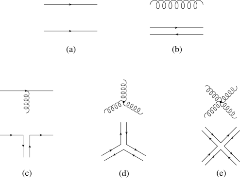
Figure 8: ’t Hooft’s double line notation. The lower diagram shows each QCD propagator or interaction vertex in the double line notation.

and the color at the beginning of the line is the same as at the end of the line, because of the $\delta^{ab}$ in eq. (16). The gluon propagator is

$$\left\langle A^{A}_{\mu}\left(x\right)A_{\nu}^{B}\left(y\right)\right\rangle=\delta^{AB}D_{\mu\nu}\left(x-y\right),$$

where $A$ and $B$ are indices in the adjoint representation. Instead of treating a gluon as a field with a single adjoint index, it is preferable to treat it as an $N\times N$ matrix with two indices in the $N$ and $\overline{N}$ representations, $\left(A_{\mu}\right)^{a}{}_{b}=A_{\mu}^{A}\left(T^{A}\right)^{a}{}_{b}$. The gluon propagator can be rewritten as

$$\left\langle A_{\mu b}^{a}\left(x\right)A_{\nu d}^{c}\left(y\right)\right\rangle=D_{\mu\nu}\left(x-y\right)\left(\frac{1}{2}\delta^{a}_{d}\,\delta^{c}_{b}-\frac{1}{2N}\delta^{a}_{b}\,\delta^{c}_{d}\right),$$

where the identity

$$\left(T^{A}\right)^{a}{}_{b}\left(T^{A}\right)^{c}{}_{d}=\frac{1}{2}\delta^{a}_{d}\,\delta^{c}_{b}-\frac{1}{2N}\delta^{a}_{b}\,\delta^{c}_{d}\qquad\left(SU(N)\right)$$ (17)

has been used. The corresponding identity for $U(N)$ is

$$\left(T^{A}\right)^{a}{}_{b}\left(T^{A}\right)^{c}{}_{d}=\frac{1}{2}\delta^{a}_{d}\,\delta^{c}_{b}\qquad\left(U(N)\right),$$ (18)

where the $U(1)$ generator has the same normalization as the $SU(N)$ generators. It is convenient to use the $U(N)$ identity eq. (18) instead of the $SU(N)$ identity eq. (17) for analyzing the $N$-dependence of Feynman diagrams. The correct $SU(N)$ propagator is given by including an additional $U(1)$ ghost field that cancels the extra $U(1)$ gauge boson in $U(N)$. The effects of the $U(1)$ gauge boson are $1/N^{2}$ suppressed, as we will see later. In most applications, the difference between $U(N)$ and $SU(N)$ will turn out to be unimportant. The reason is that, typically, what one can prove is that a certain amplitude first occurs at some order in $1/N$. For such computations, the numerical size of the $1/N$ corrections is irrelevant.

The $U(N)$ gluon propagator can then be represented using ’t Hooft’s double line notation, as in fig. 8(b). The color lines represent the $N$ and $\overline{N}$ indices $a$ and $b$ on $A_{\mu}^{a}{}_{b}$, and color is conserved during propagation because of the $\delta$-function structure in eq. (18). The gauge-fermion vertex $\overline{\psi}_{a}\,{\raise 0.6458pt\hbox{/}\mkern-14.0muA}^{a}{}_{b}\psi^{b}$ is shown in fig. 8(c). The double line notation provides a simple way to keep track of the color index contractions in a Feynman graph.

The three and four gauge boson vertices arise from the $\Tr F_{\mu\nu}F^{\mu\nu}$ gluon kinetic energy. Each kinetic energy term is a single trace over color. The three-gluon vertex arises from terms such as

$$\Tr A_{\mu}A_{\nu}\partial_{\mu}A_{\nu}=A_{\mu}^{a}{}_{b}A_{\nu}^{b}{}_{c}\partial_{\mu}A_{\nu}^{c}{}_{a},$$ (19)

where the color indices have been shown explicitly. It is represented using the double line notation as fig. 8(d), and the four gluon vertex as in fig. 8(e). It is important that all the interactions arise from a single color trace — otherwise one could have color flow in a four-gluon vertex as in fig. 9, where the diagram can be broken up into two disconnected color flows.

Figure 9: Color flow for a four-gluon interaction which has two color traces.

Every Feynman graph in the original theory can then be written as a sum of double line graphs. Each double line graph gives a particular color index contraction of the original diagram. An example of a Feynman graph and one of its double line partners is shown in fig. 10.

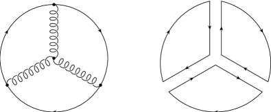
Figure 10: A Feynman graph, and one of its partner double line graphs, representing a particular color index contraction. This is an example of a planar diagram.

One Feynman graph can give rise to several double line graphs. For example, the three-gluon vertex is given by eq. (19), plus a term with $A_{\mu}\leftrightarrow A_{\nu}$. The complete three-gluon vertex in the double line notation is represented in fig. 11.

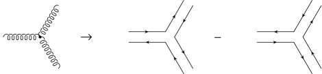
Figure 11: The complete three-gluon vertex in double line notation.

One can think of each double line graph as a surface obtained by gluing polygons together at the double lines. Since each line has an arrow on it, and double lines have oppositely directed arrow, one can only construct orientable polygons in an $SU(N)$ theory. For $SO(N)$, the fundamental representation is a real representation, and the lines do not have arrows. In this case, it is possible to construct non-orientable surfaces such as Klein bottles.

To compute the $N$-dependence requires counting powers of $N$ from sums over closed color index loops, as well as factors of $1/\sqrt{N}$ from the explicit $N$ dependence in the coupling constants. It is convenient to use a rescaled Lagrangian to simplify the derivation of the $N$-counting rules. Define rescaled gauge fields $gA/\sqrt{N}\rightarrow{\hat{A}}$ so that the covariant derivative is $D_{\mu}=\partial_{\mu}+i{\hat{A}}_{\mu}$, and rescaled fermion fields $\psi\rightarrow\sqrt{N}{\hat{\psi}}$ so that the Lagrangian becomes

$$L=N\left[-\frac{1}{2g^{2}}\Tr{\hat{F}}_{\mu\nu}{\hat{F}}^{\mu\nu}+\sum_{k=1}^{N_{F}}\overline{\hat{\psi}}_{k}\left(i\,\hbox{/\kern-6.00006ptD}-m_{k}\right){\hat{\psi}}_{k}\right].$$ (20)

The Lagrangian has an overall $N$, but the theory does not reduce to a classical theory of quarks and gluons in the $N\rightarrow\infty$ limit, because the number of components of ${\hat{\psi}}$ and ${\hat{A}}_{\mu}$ grows with $N$.

One can read off the powers of $N$ in any Feynman graph from eq. (20). Every vertex has a factor of $N$, and every propagator has a factor of $1/N$. In addition, every color index loop gives a factor of $N$, since it represents a sum over $N$ colors. In the double line notation where Feynman graphs correspond to polygons glued to form surfaces, each color index loop is the edge of a polygon, and is the face of the surface. Thus one finds that a connected vacuum graph (i.e. with no external legs) is of order

$$N^{V-E+F}=N^{\chi},$$ (21)

where $V$ is the number of vertices, $E$ is the number of edges, $F$ is the number of faces, and $\chi\equiv V-E+F$ is a topological invariant known as the Euler character. For a connected orientable surface

$$\chi=2-2h-b,$$ (22)

where $h$ is the number of handles, and $b$ is the number of boundaries (or holes). For a sphere $h=0$, $b=0$, $\chi=2$; for a torus, $h=1$, $b=0$, $\chi=0$.

A quark is represented by a single line, and so a closed quark loop is a boundary. Thus every closed quark loop brings a $1/N$ suppression. The maximum power of $N$ is two, from graphs with $h=b=0$. These are connected graphs with no closed quark loops, with the topology of a sphere. Remove one polygon from the sphere, so that one obtains a sphere with one hole. This can be flattened into a diagram drawn on a flat sheet of paper, with the hole as the outermost edge. One can then glue back the removed polygon by thinking of it as the paper exterior to the diagram with infinity identified. Thus the order $N^{2}$ graphs are planar diagrams with only gluons, that is, they can be drawn on the surface of a sheet of paper without having a gluon “jump” over another. All points where gluon lines cross have to be interaction vertices.

A diagram with $c$ connected pieces can be of order $N^{2c}$, and so grows with the number of connected pieces. This is not surprising; the sum of all diagrams is the exponential of the connected diagrams. The connected diagrams are of order $N^{2}$, corresponding to a vacuum energy of order $N^{2}$, which is to be expected since there are $\mathcal{O}\left(N^{2}\right)$ gluon degrees of freedom. Expanding the exponential gives arbitrary high powers of $N$. From now on, we will restrict $N$-counting to the connected diagrams. One can obtain the $N$ dependence of a disconnected diagram by multiplying together the $N$ dependence of all the connected pieces.

We will often be interested in correlation functions that depend on properties of the quarks, such as masses. The leading graphs that depend on quarks must have at least one quark line, and are order $N$, with $h=0$ and $b=1$. One might expect the quark contribution to the vacuum energy to be of order $N$, since there are $N$ quarks of each flavor. The order $N$ quark diagrams have the topology of a sphere with one hole, with the quark loop forming the edge of the hole. One can then flatten them out into a planar diagram as for gluons. In this case, the order $N$ diagrams are written as planar diagrams with a single quark loop which forms the outermost edge of the diagram. An example of a planar quark diagram is fig. 10. Figure 10 is of order $N$, since $h=0$ and $b=1$. This can also be seen using the original $N$-counting rules of the Lagrangian eq. (14). Each vertex has a factor $g/\sqrt{N}$, and each closed index loop brings a factor of $N$, so the graph is of order $(1/\sqrt{N})^{4}\times N^{3}=N$. Figure 12(a) is not a planar diagram, even though it can be drawn as fig. 12(b), because the diagram must be planar when drawn with the quark line as the outermost edge. Figure 12(a) is of order $1/N$, since the vertex factors give $(1/\sqrt{N})^{4}$ and the color index sum gives a factor of $N$. Note that for a given number of quark loops (boundaries $b$), the expansion is in powers of $1/N^{2}$, rather than $1/N$, because of the $-2$ in front of $h$ in eq. (22).

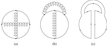
Figure 12: An example of a non-planar diagram. Diagram (a) can be redrawn as (b), but it still non-planar since the quark loop must form the outermost edge of the diagram. The double line version of the graph is shown in (c).

Large N diagrams for QCD look like two-dimensional surfaces. For example, the leading diagram in the pure-glue sector has the topology of a sphere, and the leading diagram in the quark sector is a surface with the quark as the outermost edge. One can imagine all possible planar gluon exchanges as filling out the surface into a two-dimensional world-sheet. It has been conjectured that this is the way in which large N QCD might be connected with string theory, with planar diagrams representing the leading order string theory diagrams. The topological counting rules for the $1/N$ suppression factors in QCD are the same as that for the string coupling constant in the string loop expansion. The connection between large N QCD and string theory has never been made precise. Two major obstacles are that QCD is neither supersymmetric nor conformally invariant. One result in this direction is that the partition function for $SU(N)$ Yang-Mills theory (i.e. no quarks) in two dimensions was shown to agree with the partition function of a string theory [9] by explicit calculation. The connection was possible because Yang-Mills theory in two-dimensions is a free field theory, and the partition function only depends on the topology of the background spacetime. To reproduce the correct $N$-factors, it was necessary to use a modified string theory, in which folds are suppressed.

$U(1)$ Ghosts

The corrections due to the difference between using $SU(N)$ and $U(N)$ are straightforward to analyze. As mentioned earlier, the $SU(N)$ theory can be thought of as a $U(N)$ theory with an additional $U(1)$ ghost gauge field to cancel the extra $U(1)$ gauge field in $U(N)$. The $U(1)$ ghost field does not couple to the $U(N)$ gauge bosons, since the $U(1)$ generator commutes with all the $U(N)$ generators. We only need to consider exchanges of the $U(1)$ ghost field between quark lines. The additional powers of $N$ due to the $U(1)$ ghost are most simply counted using the original form of the Lagrangian eq. (14), rather than the rescaled version eq. (20). Consider a connected diagram, with some gluon lines and ghost $U(1)$ lines. The $U(1)$ ghost does not change the color structure of the diagram, so the $N$ dependence from the color index loops, etc. is obtained using the counting rules discussed above, for the diagram with the $U(1)$ ghosts erased. In addition, one gets a factor of $1/N$ from each $U(1)$ ghost propagator (see eq. (17)), and a factor of $1/N$ from the two coupling constants at the two ends of each gauge boson line. Thus each $U(1)$ ghost brings a $1/N^{2}$ suppression. The only subtlety in this argument is that $U(1)$ exchange can turn an otherwise disconnected diagram into a connected diagram. Thus the leading diagram with one $U(1)$ ghost has two quark loops, as in fig. 13, and is order $N\times N\times 1/N^{2}=\mathcal{O}\left(1\right)$. This is only $1/N$ suppressed relative to the leading connected quark diagrams, which are order $N$. However, the effect of the $U(1)$ ghost in fig. 13 is to precisely cancel the corresponding graph with a $U(N)$ boson, since fig. 13 with $SU(N)$ boson exchange vanishes, because $\Tr T^{A}=0$. The net result is that the difference between $SU(N)$ and $U(N)$ is order $1/N^{2}$.

Figure 13: A connected diagram with one $U(1)$ ghost gauge boson exchange.

Problem 3.1

Prove eqs. (17), (18).

2 The ’t Hooft Model

The ’t Hooft model is large $N$ QCD in $1+1$ dimensions. This theory was solved by ’t Hooft [1, 2] to obtain the exact meson spectrum. There is an extensive discussion of this model in Coleman’s lectures [3]. I will not repeat the solution of the model here. Instead, I will summarize why the model is solvable, and show some of the numerical solutions.

In $1+1$ dimensions, the gauge coupling constant $g$ has dimensions of a mass, and becomes relevant in the infrared. The theory is confining, and has a linear potential at large distances. Even QED confines in $1+1$ dimensions, and has a linear potential. It is convenient to use light-cone coordinates

$$x^{\pm}=\frac{1}{\sqrt{2}}\left(x^{0}\pm x^{1}\right),$$

with metric

$$ds^{2}=2dx^{+}dx^{-},\qquad g_{\mu\nu}=\left(\begin{array}[]{cc}0&1\\ 1&0\end{array}\right),$$

and light-cone gauge $A^{+}=A_{-}=0$. The field-strength tensor has a single non-vanishing component,

$$F_{+-}=\partial_{+}A_{-}-\partial_{-}A_{+}+i{g\over\sqrt{N}}\left[A_{+},A_{-}\right]=-\partial_{-}A_{+},$$

so the theory becomes effectively Abelian. This is the first important simplification. The second is planarity, which allows one to solve the theory exactly.

Consider the quark propagator, which can be written in terms of the one-particle irreducible piece $\Sigma$, as in fig. 14.

Figure 14: The quark propagator in terms of the one-particle irreducible self-energy $\Sigma$.

The equation for $\Sigma$ is given graphically in fig. 15. Planarity is crucial for the derivation of this relation. We earlier derived the $N$-counting rules only for vacuum graphs. The results can easily be extended to the fermion two-point function, which is obtained by differentiating a vacuum graph once with respect to a fermion bilinear source, i.e., by cutting the closed quark loop at one point. Planarity of the vacuum graphs then implies that the quark propagator is given by planar graphs with all gluons on one side of the quark line. The first gluon emitted by the quark must be the last gluon absorbed, because the diagram is planar, and there are no gluon self-interactions. This immediately leads to fig. 15.

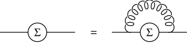
Figure 15: The equation for $\Sigma$.

The equation for $\Sigma$ in fig. 15 can be iterated, to give the solution fig. 16 for the quark propagator.

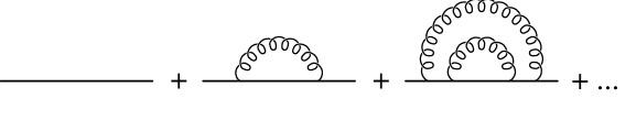
Figure 16: Rainbow sum for the exact quark propagator.

The diagrams in fig. 16 are known as rainbow diagrams, and the rainbow approximation is exact in the ’t Hooft model. The analytical solution of fig. 15 is straightforward [3]. The solution is that the quark propagator is given by the free-quark form $1/\left(\raise-0.6458pt\hbox{/}\mkern-9.5mup-M\right)$, with the renormalized quark mass $M$ given in terms of the bare quark mass by

$$M^{2}=m^{2}-{g^{2}\over 2\pi}.$$

Note that there is still a pole in the quark propagator, even though the theory is confining, and there are no quark states in the spectrum of the theory. Also note that the pole in the quark propagator can be tachyonic if $m^{2}<g^{2}/2\pi$. Nevertheless, the theory has a sensible meson spectrum for all values of $m^{2}\geq 0$.

The meson propagator has the exact graphical expansion in fig. 17,

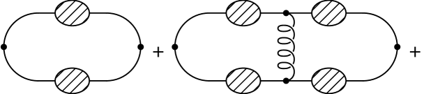
Figure 17: Graphical expansion for the meson propagator. The shaded blobs are full quark propagators.

and the ladder graph approximation is exact in the large $N$ limit. This again follows trivially from the planar diagram structure of the theory and the absence of gluon self interactions: gluons are not allowed to cross in any graph. The Bethe-Salpeter equation for the meson wavefunction, known as the ’t Hooft equation, is shown graphically in fig. 18,

Figure 18: The Bethe-Salpeter equation for the meson wavefunction. The cross-hatched blob is the meson wavefunction $\phi(x)$.

and follows from the meson propagator fig. 17. Let $P$ be the total momentum of the meson, $q$ be the momentum of the quark (the quark is well-defined, since there is no pair creation in the large $N$ limit), $x=q_{-}/P_{-}$, and $\phi(x)$ the amplitude to find the quark with this light-cone momentum fraction. A simple calculation leads to the ’t Hooft equation [1, 2, 3] for the meson wavefunction

$$\mu^{2}\phi(x)=\left[{M_{1}^{2}\over x}+{M_{2}^{2}\over 1-x}\right]\phi(x)-{g^{2}\over 2\pi}\int_{0}^{1}dy\ P\left({1\over(x-y)^{2}}\right)\phi(y),$$

where $P$ denotes the principal value, $\mu$ is the meson mass, $M_{1}$ is the renormalized quark mass, and $M_{2}$ is the renormalized antiquark mass.

This equation can be solved numerically using a Multhopp transform [10]. The ground state wavefunction $\phi(x)$ for $m_{1}=m_{2}=1$ (renormalized masses in units of $g/\sqrt{2\pi}$) is shown in fig. 19. The meson mass is $\mu=2.7$, which is larger than the sum of the two quark masses. The wavefunction of the first excited state is shown in fig. 20, and corresponds to a meson with mass $\mu=4.16$. One can show that for large excitation number $n$, the meson mass is linear in $n$. The ground state wavefunction for $m_{1}=m_{2}=10$ is shown in fig. 21; the meson mass is $\mu=20.55$. Clearly, increasing the quark mass narrows the momentum spread in the wavefunction, and also decreases $\mu-m_{1}-m_{2}$, the strong interaction contribution to the mass. For unequal masses, the momentum distribution is asymmetric, and the heavy quark carries most of the momentum. Figure 22 shows the ground state wavefunction for $m_{1}=5$, $m_{2}=1$, with a meson mass $\mu=6.72$. For light quarks, $m\rightarrow 0$, the meson wavefunction is not affected much by the quark mass. As one might expect, the structure of the wavefunction is governed by the scale $g$ rather than $m$. The wavefunctions of the ’t Hooft model show many of the features one would expect for the wavefunctions of mesons in QCD in $3+1$ dimensions.

Figure 19: The ground state wavefunction of the ’t Hooft model with $m_{1}=m_{2}=1$.

Figure 20: The wavefunction for the first excited state of the ’t Hooft model with $m_{1}=m_{2}=1$.

Figure 21: The ground state wavefunction of the ’t Hooft model with $m_{1}=m_{2}=10$.

Figure 22: The ground state wavefunction of the ’t Hooft model with $m_{1}=5$ and $m_{2}=1$.

3 $N$-Counting Rules for Correlation Functions

We have discussed the $N$-counting rules for connected vacuum diagrams. These can be used to derive $N$-counting rules for gluon and quark correlation functions. The correlators we will study are vacuum expectation values of products of gauge invariant quark and gluon operators. The operators need not be local; all we require is that they cannot be split into pieces which are separately color singlets. Allowed operators are

$$\overline{\hat{\psi}}{\hat{\psi}},\ {\hat{F}}_{\mu\nu}{\hat{F}}^{\mu\nu},\ \overline{\hat{\psi}}D^{\mu}{\hat{\psi}},\ \overline{\hat{\psi}}{\hat{F}}^{\mu\nu}{\hat{\psi}},\ \overline{\hat{\psi}}(y)Pe^{-i\int_{x}^{y}{\hat{A}}_{\mu}dz^{\mu}}{\hat{\psi}}(x),$$

but not

$$\left(\overline{\hat{\psi}}{\hat{\psi}}\right)^{2}.$$

Operators involving quark fields must be bilinear in the quarks. Let ${\hat{O}}_{i}$ denote a generic operator written in terms of rescaled fields, and add the source term $NJ_{i}{\hat{O}}_{i}$ to the rescaled Lagrangian eq. (20). The entire Lagrangian still has an overall factor of $N$, so the $N$-counting rule eq. (21) still holds. Connected correlation functions are then obtained by differentiating $W(J)$, the sum of connected vacuum graphs, with respect to the sources

$$\left\langle{\hat{O}}_{1}{\hat{O}}_{2}\ldots{\hat{O}}_{r}\right\rangle_{C}={1\over iN}{\partial\over\partial J_{1}}\ldots{1\over iN}{\partial\over\partial J_{r}}W(J).$$

The order $N^{2}$ contribution to $W(J)$ is from graphs with only gluon lines. This can contribute to the correlation function $\langle{\hat{O}}_{1}{\hat{O}}_{2}\ldots{\hat{O}}_{r}\rangle_{C}$, provided none of the operators contain any quark fields. Thus pure-gluon $r$-point correlation functions are of order $N^{2-r}$. The diagrams that contribute to these are planar diagrams with insertions of ${\hat{O}}_{i}$. The first contribution to $W(J)$ that involves quarks is of order $N$. Thus $r$-point correlation functions that involve quark fields are of order $N^{1-r}$. The diagrams that contribute to them are planar diagrams with a single quark loop with the fermion bilinears inserted on the quark line, as shown in fig. (23).

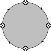
Figure 23: Leading contribution to a quark correlation function. The shaded region represents planar gluons, and $\otimes$ are insertions of the fermion bilinears ${\hat{O}}_{i}$.

The $N$-counting rules were derived using the rescaled Lagrangian eq. (20). One can obtain $N$-counting rules for correlation functions with fields normalized as in the original Lagrangian eq. (14) by using the replacement

$$\psi=\sqrt{N}{\hat{\psi}},\ A={\sqrt{N}\over g}{\hat{A}}.$$ (23)

In particular, quark bilinears are related by a factor of $N$, $O_{i}=N{\hat{O}}_{i}$, e.g. $\overline{\psi}\psi=N\overline{\hat{\psi}}{\hat{\psi}}$.

The $N$-counting rules for correlation functions can be used to derive the $N$-counting rules for meson and glueball scattering amplitudes. We will use the notation ${\hat{G}}_{i}$ to denote a gauge invariant pure-gluonic operator, and ${\hat{H}}_{i}$ to denote a gauge invariant operator bilinear in the quark fields, where the operators are written in terms of the rescaled fields. Gluon operators ${\hat{G}}_{i}$ can create glueballs, and quark bilinears ${\hat{H}}_{i}$ can create mesons. The two point function $\langle{\hat{G}}_{1}{\hat{G}}_{2}\rangle_{c}$ is of order unity, so ${\hat{G}}_{i}$ creates glueball states with unit amplitude. The $r$-point function $\langle{\hat{G}}_{1}\ldots{\hat{G}}_{r}\rangle_{c}$ is of order $N^{2-r}$. Thus $r$-glueball interaction vertices are of order $N^{2-r}$, and each additional glueball gives a $1/N$ suppression. The meson two point correlation function $\langle{\hat{H}}_{1}{\hat{H}}_{2}\rangle_{c}\sim 1/N$. Thus $\sqrt{N}{\hat{H}}_{i}$ creates a meson with unit amplitude. The $r$-point function $\langle\sqrt{N}{\hat{H}}_{1}\ldots\sqrt{N}{\hat{H}}_{r}\rangle_{c}$ is of order $N^{1-r/2}$. Thus $r$-meson interaction vertices are of order $N^{1-r/2}$, and each additional meson gives a $1/\sqrt{N}$ suppression. Finally, one can look at mixed glue-ball meson correlators, $\langle{\hat{G}}_{1}\ldots{\hat{G}}_{r}{\hat{H}}_{1}\ldots{\hat{H}}_{s}\rangle_{c}$, which are of order $N^{1-r-s}$. Thus an interaction vertex involving $r$ glueballs and $s$ mesons is of order $N^{1-r-s/2}$, so that $\langle{\hat{G}}\sqrt{N}{\hat{H}}\rangle$ is of order $1/\sqrt{N}$ — meson-glueball mixing is of order $1/\sqrt{N}$, and vanishes in the $N\rightarrow\infty$ limit.

One important result that we will need later is that the pion decay constant $f_{\pi}$ is of order $\sqrt{N}$. The matrix element $\langle{0}\vphantom{\overline{q}\gamma^{\mu}\gamma_{5}T^{a}q\pi^{b}(p)}|{\overline{q}\gamma^{\mu}\gamma_{5}T^{a}q}|\vphantom{0\overline{q}\gamma^{\mu}\gamma_{5}T^{a}q}{\pi^{b}(p)}\rangle=if_{\pi}p^{\mu}\delta^{ab}$, where the quark fields are normalized as in the original Lagrangian eq. (14). The $N$-dependence of the matrix element can be obtained from $\langle{\hat{H}}_{1}\sqrt{N}{\hat{H}}_{2}\rangle\sim\mathcal{O}(1/\sqrt{N})$, where the first bilinear is the axial current, and the second bilinear produces a pion from the vacuum with amplitude of order unity. One needs to multiply ${\hat{H}}_{1}$ by an additional factor of $N$ to convert the axial current from rescaled fields to the original quark fields, so that

$$f_{\pi}\propto\sqrt{N}.$$

The $N$-counting rules imply that one has a weakly interacting theory of mesons and glueballs with a coupling constant $1/\sqrt{N}$. As in any weakly interacting theory, one can expand in the coupling constant $1/\sqrt{N}$. The leading order graphs are tree-graphs, and the leading order singularities are poles. At one-loop (i.e. $1/N$), one gets 2 particle cuts, at two loops, three-particle cuts, and so on. QCD, a strongly interacting theory of quarks and gluons, has been rewritten as a weakly interacting theory of hadrons. The leading (in $N$) interactions bind the quarks and gluons into color singlet hadrons. The residual interactions between these hadrons are $1/N$ suppressed. The $1/N$ expansion is also equivalent to the semiclassical expansion for the meson theory. These results will also hold for baryons.

The spectrum of the theory contains an infinite number of narrow glueball and meson resonances. The resonances are narrow, because their decay widths vanish as $N\rightarrow\infty$, since all decay vertices are proportional to powers of the weak coupling constant $1/\sqrt{N}$ and hadron masses (i.e. phase space factors) do not grow with $N$. There must be an infinite number of resonances to reproduce the logarithmic running of QCD correlation functions. A meson two-point correlation function can be written as a sum over resonances,

$$\int d^{4}xe^{iq\cdot x}\left\langle Q(x)Q(0)\right\rangle_{C}=\sum_{i}{Z_{i}\over q^{2}-m_{i}^{2}},$$

since single meson exchange dominates in the large $N$ limit. The left hand side has logarithms of $q^{2}$, which can only be reproduced by the right hand side if there are an infinite number of terms in the sum.

4 The Master Field

The $N$-counting rules imply that the functional integral measure is concentrated on a single gauge orbit, and that fluctuations vanish in the $N\rightarrow\infty$ limit. For example, if ${\hat{G}}$ is a gauge invariant operator made of gluon fields, $\langle{\hat{G}}\rangle\sim\mathcal{O}(N)$, and its variance is

$$\left(\Delta{\hat{G}}\right)^{2}\sim\left\langle{\hat{G}}^{2}\right\rangle-\left\langle{\hat{G}}\right\rangle^{2}=\left\langle{\hat{G}}^{2}\right\rangle_{c}\sim\mathcal{O}(1).$$

Thus $\Delta{\hat{G}}/{\hat{G}}\sim\mathcal{O}(1/N)\rightarrow 0$. It is easy to see that all gauge invariant observables have no fluctuations in the $N\rightarrow\infty$ limit. The functional integral measure must then be concentrated on a single gauge orbit, known as the master orbit, represented by a set of gauge equivalent vector potentials $A_{\mu}(x)$. It is expected that one can find a point on this orbit where the vector potential is given by constant matrices $A_{\mu}$. This is the master field, and all correlation functions are given by computing them in this single field configuration. A lot of information can be encoded in the master field, since it is an $\infty\times\infty$ matrix. The master field has recently been determined for QCD in $1+1$ dimensions [11, 12].

There are some other interesting results for large $N$ QCD in $1+1$ dimensions which have been obtained recently. The basic gauge invariant observables in a gauge theory are the Wilson loops. Kazakov and Kostov obtained the exact expression for all Wilson loops [13]. The Wilson loop for a close curve $C$ is the expectation value of the trace of the path-ordered exponential

$$W(C)=\left\langle\Tr Pe^{-ig\int A_{\mu}\ dx^{\mu}}\right\rangle,$$ (24)

and is of order $N$. For a simple closed curve, the Wilson loop for $1+1$ dimensional large $N$ QCD satisfies an exact area law,

$$W(C)=N\,e^{-g^{2}A/2},$$

where $A$ is the area enclosed by $C$. More interesting examples are self-intersecting curves, such as those in fig. 24,

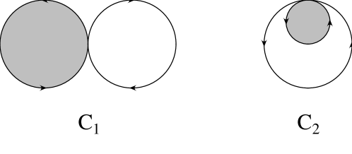
Figure 24: Examples of Wilson loops. $A_{1}$ and $A_{2}$ are the unshaded and shaded areas, respectively.

with Wilson loops

$$W(C_{1})=N\,e^{-g^{2}\left(A_{1}+A_{2}\right)/2},\qquad W(C_{2})=N\,e^{-g^{2}\left(A_{1}+2A_{2}\right)/2}\left[1-g^{2}A_{2}\right],$$

where $A_{1}$ and $A_{2}$ are the unshaded and shaded areas, respectively. The master field for 2D QCD has been shown to reproduce the Kazakov-Kostov results for the Wilson loops.

Problem 3.2

In a non-Abelian theory, the field strength tensor $F_{\mu\nu}$ does not determine all the gauge invariants. In $1+1$ dimensions for gauge group $SU(2)$, construct two different vector potentials which both produce the same constant field strength tensor $F_{12}=f\tau_{3}$, where $f\not=0$ is a constant, and yet give different values for Wilson loops.

Problem 3.3

Define the matrix

$$U_{R}=Pe^{-ig\int A_{\mu}\ dx^{\mu}}$$

where $A_{\mu}=A_{\mu}^{A}T^{A}$ with $T^{A}$ in representation $R$ of $SU(N)$. The Wilson loop in the fundamental representation (denoted by $F$), eq. (24), is

$$W_{F}(C)=\left\langle\Tr U_{F}\right\rangle$$

where $\left\langle\cdot\right\rangle$ represents a functional integral over all gauge field configurations. Show that the Wilson loop in the adjoint representation is

$$W_{\rm adj}(C)=\left\langle\Tr U_{\rm adj}\right\rangle=\left\langle\Tr U_{F}\Tr U^{\dagger}_{F}\right\rangle-1.$$

This equation holds in any number of dimensions, and does not depend on taking the large $N$ limit. The Wilson loop $W_{F}(C)$ is expected to have an area law,

$$W_{F}(C)\sim N\,\exp(-\lambda\ {\rm area(C)}),$$

where $\lambda$ is an unknown constant. Show that in the large $N$ limit, one expects [14]

$$W_{\rm adj}(C)\sim N^{2}\,\exp(-2\ \lambda\ {\rm area(C)})+\exp(-\lambda^{\prime}\ {\rm perimeter(C))},$$

where $\lambda^{\prime}$ is another unknown constant. What are the implications of this formula for confinement/screening of adjoint quarks?

4 Meson Phenomenology

1 Zweig’s Rule

Meson correlation functions at leading order in $1/N$ are given by diagrams with a single quark loop. Annihilation graphs, such as those in fig. 25,

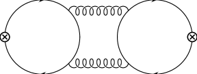
Figure 25: An annihilation graph, which violates Zweig’s rule and is $1/N$ suppressed.

have two quark loops and are suppressed by one power of $N$. The suppression of annihilation graphs is known as Zweig’s rule. One consequence of this is that mesons occur in nonets for three light quark flavors. There are nine possible $\overline{q}q$ states, which are divided into flavor octets $\overline{q}\,T^{A}\,q$, where $T^{A}$ is a $SU(3)$ flavor matrix, and a singlet $\overline{q}q$. Usually, the singlet and octet mesons are not related, because the singlet meson can mix with gluons. In the large $N$ limit, this mixing is suppressed. The singlet and octet meson couplings are related by treating them as members of a $U(N)$ multiplet, with the $U(1)$ and $SU(N)$ couplings having the same normalization. Examples of this are: in the large $N$ limit, the vector meson nonet of $\left\{\rho,\omega,\phi,K^{*}\right\}$ all have the same mass, and the decay constants of the $\pi$ and $\eta^{\prime}$ are equal, $f_{\pi}=f_{\eta^{\prime}}$.

2 Exotics

At leading order in $1/N$, there are no exotic states. This does not mean that there are no exotic states in QCD, only that their binding is subleading in the $1/N$ expansion. As an example, consider the propagator $\langle\left(\overline{q}q\right)^{2}\left(\overline{q}q\right)^{2}\rangle$ for a four-quark state $\overline{q}q\overline{q}q$. It is easy to see that at leading order, the graphs which contribute have the form shown in fig. 26,

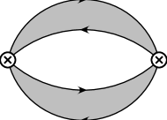
Figure 26: The leading order graphs for the $\left\langle\left(\overline{q}q\right)^{2}\left(\overline{q}q\right)^{2}\right\rangle$ correlation function. The shaded regions represent planar gluons.

i.e. the correlation function is $\left\langle\overline{q}q\ \overline{q}q\right\rangle^{2}$, the square of the $\overline{q}q$ correlation function. This is the correlation function for two non-interacting mesons, and so $\left(\overline{q}q\right)^{2}$ creates two mesons, rather than a four-quark state.

3 Chiral Perturbation Theory

The $U(N_{F})_{L}\times U(N_{F})_{R}$ chiral symmetry symmetry of QCD is spontaneously broken to a diagonal $U(N_{F})_{V}$ vector symmetry, resulting in (pseudo-) Goldstone bosons. This form for the breaking can be proved in the large $N$ limit [15]. The low-energy interactions of the pseudo-Goldstone bosons of QCD, the $\pi$, $K$, $\eta$, and $\eta^{\prime}$, can be described in terms of an effective Lagrangian known as the chiral Lagrangian. One can imagine computing the chiral Lagrangian by evaluating the QCD functional integral with sources for the pseudo-Goldstone bosons. The source terms are fermion bilinears. In the large $N$ limit, we have seen that the leading order diagrams that contribute to correlation functions of fermion bilinears are of order $N$, and contain a single quark loop, as in fig. 23. This implies that the leading order terms in the chiral Lagrangian are of order $N$. It is also clear from the structure of fig. 23 that the leading order terms can be written as a single flavor trace, since the outgoing quark flavor at one vertex is the incoming flavor at the next vertex. Similarly, diagrams with two quark loops have two flavor traces, and are of order unity, and in general, those with $r$ quark loops have $r$ traces, and are of order $N^{1-r}$.

The chiral Lagrangian is written in terms of a unitary matrix

$$U=e^{2i\Pi/f_{\pi}},$$ (25)

where $f_{\pi}\approx 93$ MeV is the pion decay constant, and

$$\Pi={1\over\sqrt{2}}\left(\begin{array}[]{ccc}{\pi^{0}\over\sqrt{2}}+{\eta\over\sqrt{6}}+{\eta^{\prime}\over\sqrt{3}}&\pi^{+}&K^{+}\\[7.5pt] \pi^{-}&-{\pi^{0}\over\sqrt{2}}+{\eta\over\sqrt{6}}+{\eta^{\prime}\over\sqrt{3}}&K^{0}\\[7.5pt] K^{-}&{\overline{K}}^{0}&-{2\eta\over\sqrt{6}}+{\eta^{\prime}\over\sqrt{3}}\\ \end{array}\right),$$ (26)

is the matrix of pseudo-Goldstone bosons. The $\eta^{\prime}$ has been included, since it is related to the octet pseudo-Goldstone bosons in the large $N$ limit, by Zweig’s rule. The order $p^{2}$ terms in the chiral Lagrangian are

$$L^{(2)}={f^{2}_{\pi}\over 4}\Tr D^{\mu}UD_{\mu}U^{-1}+{f^{2}_{\pi}\over 4}B\Tr\left(m^{\dagger}U+mU^{-1}\right),$$ (27)

where $m$ is the quark mass matrix in the QCD Lagrangian. The first term is order $N$, since $f_{\pi}\propto\sqrt{N}$. The second term in eq. (27) also has a single trace and is of order $N$, so $B$ is of order unity. The $U$ field has an expansion in powers of $\pi/f_{\pi}$. Thus each additional meson field has a factor of $1/f_{\pi}\propto 1/\sqrt{N}$, which gives the required $1/\sqrt{N}$ suppression for mesons derived earlier. The effective Lagrangian eq. (27) has an overall factor of $N$, and the $U$ matrix is $N$ independent, so the $1/N$ expansion is equivalent to a semiclassical expansion. Graphs computed using the chiral Lagrangian have a $1/N$ suppression for each loop.

The order $p^{4}$ terms in the chiral Lagrangian are conventionally written as [16]

$$L^{(4)}=L_{1}\left[\Tr D_{\mu}U^{-1}D^{\mu}U\right]^{2}+L_{2}\Tr D_{\mu}U^{-1}D_{\nu}U\Tr D^{\mu}U^{-1}D^{\nu}U$$

$$+L_{3}\Tr D_{\mu}U^{-1}D^{\mu}UD_{\nu}U^{-1}D^{\nu}U$$

$$+L_{4}\Tr D_{\mu}U^{-1}D^{\mu}U\Tr\left(U^{-1}m+m^{\dagger}U\right)$$

$$+L_{5}\Tr D_{\mu}U^{-1}D^{\mu}U\left(U^{-1}m+m^{\dagger}U\right)+L_{6}\left[\Tr\left(U^{-1}m+m^{\dagger}U\right)\right]^{2}$$

$$+L_{7}\left[\Tr\left(U^{-1}m-m^{\dagger}U\right)\right]^{2}+L_{8}\Tr\left(m^{\dagger}Um^{\dagger}U+U^{-1}mU^{-1}m\right)$$

$$-iL_{9}\Tr\left(F^{\mu\nu}_{R}D_{\mu}UD_{\nu}U^{-1}+F^{\mu\nu}_{L}D_{\mu}U^{-1}D_{\nu}U\right)$$

$$+L_{10}\Tr U^{\dagger}F^{\mu\nu}_{R}U^{-1}F_{L\mu\nu},$$ (28)

where $F_{L,R}$ are the field-strength tensors of the (flavor) $U(3)_{L}$ and $U(3)_{R}$ gauge fields. The terms with a single trace, $L_{3}$, $L_{5}$, $L_{8}$, $L_{9}$ and $L_{10}$ should be of order $N$, and those with two traces, $L_{1}$, $L_{2}$, $L_{4}$, $L_{6}$ and $L_{7}$ should be of order one. This is not correct, because of one subtlety. There is an identity

$$\Tr ABAB=-2\Tr A^{2}B^{2}+\frac{1}{2}\Tr A^{2}\Tr B^{2}+\left(\Tr AB\right)^{2},$$ (29)

which is valid for arbitrary traceless $3\times 3$ matrices $A$ and $B$. Using $A=D_{\mu}UU^{-1}$ and $B=D_{\nu}UU^{-1}$ in eq. (29) gives the relation

$$\Tr D_{\mu}UD_{\nu}U^{-1}D^{\mu}UD^{\nu}U^{-1}=-2\Tr D_{\mu}UD^{\mu}U^{-1}D_{\nu}UD^{\nu}U^{-1}$$

$$+\frac{1}{2}\Tr D_{\mu}UD^{\mu}U^{-1}\Tr D_{\nu}UD^{\nu}U^{-1}+\Tr D_{\mu}UD_{\nu}U^{-1}\Tr D^{\mu}UD^{\nu}U^{-1}.$$

(30)

It is important to remember that this relation is special to three flavors, and would not hold for an arbitrary number of flavors. The operator $\Tr D_{\mu}UD_{\nu}U^{-1}D^{\mu}UD^{\nu}U^{-1}$ is a single trace operator and can occur in the Lagrangian with a coefficient $c$ which is of order $N$. Eliminating the operator using the identity eq. (30) gives the contributions $\delta L_{1}=c/2$, $\delta L_{2}=c$ and $\delta L_{3}=-2c$ to $L_{1-3}$. $L_{3}$ was already of order $N$, and so remains order $N$. $L_{1}$ and $L_{2}$ are now of order $N$, because of the $c$ term, but $2L_{1}-L_{2}$ is of order unity. Thus one finds the $N$-counting rules

$$\mathcal{O}(N): L_{1},L_{2},L_{3},L_{5},L_{8},L_{9},L_{10}$$

$$\mathcal{O}(1): 2L_{1}-L_{2},L_{4},L_{6},L_{7}$$

These are the $N$-counting rules given in ref. [16], with the exception of $L_{7}$, which is taken from ref. [17]. In ref. [16], $L_{7}$ was argued to be of order $N^{2}$. We will return to $L_{7}$ in section 7, after discussing the $\eta^{\prime}$. The experimental values for the $L$’s are given in Table 1. The terms of order $N$ are systematically larger than those of order unity.

Table 1: Experimental values for the coefficients of the order $p^{4}$ terms in the chiral Lagrangian, eq. (28). Values are from ref. [18]

$L_{i}$	Value			Order
$2L_{1}-L_{2}$	$-0.6$	$\pm$	$0.5$	$1$
$L_{4}$	$-0.3$	$\pm$	$0.5$	$1$
$L_{6}$	$-0.2$	$\pm$	$0.3$	$1$
$L_{7}$	$-0.4$	$\pm$	$0.2$	$1$
$L_{2}$	$1.4$	$\pm$	$0.3$	$N$
$L_{3}$	$-3.5$	$\pm$	$1.1$	$N$
$L_{5}$	$1.4$	$\pm$	$0.5$	$N$
$L_{8}$	$0.9$	$\pm$	$0.3$	$N$
$L_{9}$	$6.9$	$\pm$	$0.7$	$N$
$L_{10}$	$-5.5$	$\pm$	$0.7$	$N$

Higher derivative terms in the chiral Lagrangian are suppressed by powers of the chiral symmetry breaking scale $\Lambda_{\chi}\sim 1$ GeV [19, 20]. In the large $N$ limit, $\Lambda_{\chi}$ is of order unity, and so stays at around $1$ GeV. Loop graphs in the chiral Lagrangian are proportional to $1/(4\pi f_{\pi})^{2}$ and are of order $1/N$. Thus in the large $N$ limit, the chiral Lagrangian can be used at tree level, and loop effects are suppressed by powers of $1/N$.

4 Non-leptonic $K$ Decay

Weak decays of hadrons can be computed in terms of an effective low energy Lagrangian, since hadron masses are much smaller than the $W$ mass. Semileptonic weak decays, such as $K\rightarrow\pi\ell\nu$, can be computed using the weak Lagrangian

$$L=-{4G_{F}\over\sqrt{2}}\ \overline{u}\gamma^{\mu}P_{L}s\,\overline{\ell}\gamma_{\mu}P_{L}\nu,$$

where $P_{L}=(1-\gamma_{5})/2$ is the left-handed projection operator. To all orders in the strong interactions (and neglecting electromagnetic corrections), the matrix element for the decay $H_{i}\rightarrow H_{f}\ell\overline{\nu}$ can be written as

$$-i{4G_{F}\over\sqrt{2}}\left\langle{H_{f}}\vphantom{\overline{u}\gamma^{\mu}P_{L}sH_{i}}\right|{\overline{u}\gamma^{\mu}P_{L}s}\left|\vphantom{H_{f}\overline{u}\gamma^{\mu}P_{L}s}{H_{i}}\right\rangle\left\langle{\ell\overline{\nu}}\vphantom{\overline{\ell}\gamma_{\mu}P_{L}\nu 0}\right|{\overline{\ell}\gamma_{\mu}P_{L}\nu}\left|\vphantom{\ell\overline{\nu}\overline{\ell}\gamma_{\mu}P_{L}\nu}{0}\right\rangle,$$

i.e. it factorizes into the product of a hadronic matrix element, and a leptonic matrix element. The leptonic part can be computed explicitly using free Dirac spinors. The hadronic part is the matrix element of a current, and for $K$ decays, it can be computed in terms of the decay constant $f_{K}$. The decay constant is determined from the measured $K\rightarrow\mu\overline{\nu}$ decay rate, and can then be used to predict other decay rates such as $K\rightarrow\pi e\overline{\nu}$, etc.

Non-leptonic $K$ decay amplitudes are more difficult to compute, since they depend on the hadronic matrix elements of four-quark operators. To analyze these using the large $N$ limit, it is convenient to first look at the weak amplitudes directly in terms of $W$ exchange, rather than using the effective weak Lagrangian. The $K\rightarrow\pi\pi$ amplitude in the large $N$ limit, and to lowest order in the electroweak interactions, is given by diagrams with a single $W$ boson. The $W$ boson is color neutral, so the $N$-counting for a diagram with a $W$ boson is the same as that for the diagram with the $W$ boson removed. The diagram must contain a quark loop, since the $K$ and $\pi$ mesons contain quarks. The leading order diagrams are planar diagrams with two quark loops (fig. 27(a)).

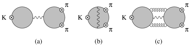
Figure 27: Diagrams for $K\rightarrow\pi\pi$. There are related diagrams with $K\leftrightarrow\pi$. The shaded regions represent planar gluons. The wavy line is the $W$ boson. The $\otimes$ are insertions of the axial current. Diagram (a) is of order $N^{2}$. The factorization violation contributions (b) and (c) are order $N$ and order unity, respectively.

These are disconnected diagrams when the $W$ boson is removed, so each quark loop subgraph is of order $N$, and the overall graph is of order $N^{2}$. The $K\rightarrow\pi\pi$ amplitude is order $\sqrt{N}$, since each current produces a meson with amplitude $\sqrt{N}$. This should be compared with a three-meson amplitude in the strong interactions, which is $1/\sqrt{N}$. Weak interaction perturbation theory is an expansion in $G_{F}\Lambda_{\rm QCD}^{2}N$. Formally, this diverges if one takes $N\rightarrow\infty$ with $G_{F}$ fixed. This does not mean that one should add lots of $W$’s to strong interaction processes to get an amplitude that grows with $N$. In the end, the results are going to be applied to $N=3$, with $G_{F}$ set to its experimental value. One can first use perturbation theory in $G_{F}$ to write the weak decay amplitudes in terms of hadronic matrix elements, and then apply the $1/N$ expansion to evaluate the purely strong interaction matrix elements.

There are no gluon exchanges between the two quark loops, so the leading order $K\rightarrow\pi\pi$ amplitude fig. 27(a) has clearly factorized into the product of $\left\langle{0}\vphantom{j^{\mu}_{W}K}\right|{j^{\mu}_{W}}\left|\vphantom{0j^{\mu}_{W}}{K}\right\rangle\times\left\langle{\pi\pi}\vphantom{j_{\mu W}0}\right|{j_{\mu W}}\left|\vphantom{\pi\pi j_{\mu W}}{0}\right\rangle$ plus terms with $\pi\leftrightarrow K$, where $j^{\mu}_{W}$ is the weak current. Factorization is exact in the large $N$ limit. Corrections to the factorization approximation, such as figs. 27(b,c) are suppressed by $1/N$ and $1/N^{2}$, respectively. The $K\rightarrow\pi\pi$ amplitudes can be computed in terms of $f_{K}$ in the factorization approximation, since each hadronic matrix element is that of a current. In particular, the ratio $A_{1/2}/A_{3/2}$ of the $\Delta I=1/2$ and $\Delta I=3/2$ amplitudes is equal to $\sqrt{2}$. One easy way to compute this is to note that the amplitude for $K^{0}\rightarrow\pi^{0}\pi^{0}$ from fig. 27(a) vanishes, since all the mesons are neutral, and the $W$ boson is charged.

Experimentally, $A_{1/2}/A_{3/2}\approx 21$, which is the famous $\Delta I=1/2$ rule in non-leptonic $K$ decays. There is no $\Delta I=1/2$ enhancement at leading order in the $1/N$ expansion [21, 22]. At first sight, this is a disaster. However, it is important to keep in mind that non-leptonic weak decays are a multiscale problem, and involve both $M_{W}$ and $\Lambda_{\rm QCD}$. Renormalization group scaling of the effective weak Lagrangian from $M_{W}$ to a low scale $\mu\sim 1$ GeV produces an enhancement of the $\Delta I=1/2$ amplitude. Formally, this enhancement is $1/N\times\log M_{W}/\mu$. $N=3$ and $\log M_{W}/\mu\sim 4$, so one should sum all powers $1/N\times\log M_{W}/\mu$. This is done by using the renormalization group to scale the weak Hamiltonian down to some low scale $\mu$ of order the the hadronic scale. Matrix elements of the low-energy weak Hamiltonian do not contain any large logarithms, and should have $1/N$ corrections of canonical size. This has been examined in detail, and is claimed to produce a satisfactory understanding of the $\Delta I=1/2$ rule [23]. The analysis is involved and will not be repeated here. A simpler example is considered in the next section.

Problem 4.1

The $K$ decay amplitudes are

$$\mathcal{A}\left(K^{+}\rightarrow\pi^{+}\pi^{0}\right) = {3\over 2}A_{3/2}$$

$$\mathcal{A}\left(K^{0}\rightarrow\pi^{+}\pi^{-}\right) = A_{1/2}+{1\over\sqrt{2}}A_{3/2}$$

$$\mathcal{A}\left(K^{0}\rightarrow\pi^{0}\pi^{0}\right) = A_{1/2}-\sqrt{2}A_{3/2},$$

neglecting final state interaction phases. Compute the amplitudes $K^{+}\rightarrow\pi^{+}\pi^{0}$, $K^{0}\rightarrow\pi^{+}\pi^{-}$, and $K^{0}\rightarrow\pi^{0}\pi^{0}$ in the factorization approximation, and use these to obtain $A_{3/2}$ and $A_{1/2}$. Compute the decay widths for $K^{+}$ and $K_{S}^{0}$ decay, and compare with experiment to obtain $A_{3/2}$ and $A_{1/2}$. Note that $K_{S}^{0}\not=K^{0}$.

5 $K-\overline{K}$ mixing

The $K-\overline{K}$ mixing amplitude is of second order in the weak interactions. The mixing amplitude is given by the matrix element of the $\Delta S=2$ Lagrangian between $K$ and $\overline{K}$. The $\Delta S=2$ Lagrangian is

$$L={G_{F}^{2}\over 16\pi^{2}}\eta(\mu)\ \overline{d}\gamma^{\mu}P_{L}s\,\overline{d}\gamma^{\mu}P_{L}s,$$ (31)

where $\eta$ has dimension two, can be computed in perturbation theory, and includes renormalization group scaling from $M_{W}$ down to some hadronic scale $\mu$. The $\mu$ dependence of $\eta$ is cancelled by the anomalous dimension of the four-quark operator. It is conventional to write the $K-\overline{K}$ matrix element of the four-quark operator as

$$\left\langle{\overline{K}}\vphantom{\overline{d}\gamma^{\mu}P_{L}s\,\overline{d}\gamma^{\mu}P_{L}sK}\right|{\overline{d}\gamma^{\mu}P_{L}s\,\overline{d}\gamma^{\mu}P_{L}s}\left|\vphantom{\overline{K}\overline{d}\gamma^{\mu}P_{L}s\,\overline{d}\gamma^{\mu}P_{L}s}{K}\right\rangle=\frac{4}{3}f_{K}^{2}M_{K}^{2}B_{K}(\mu),$$

where $B_{K}(\mu)$ parameterizes the hadronic matrix element of the four-quark operator renormalized at $\mu$. In the large $N$ limit, the matrix element is given by fig. 28(a),

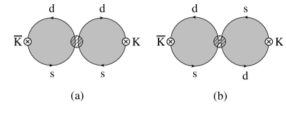
Figure 28: $K-\overline{K}$ mixing diagrams. The blob represents the four-quark operator $\overline{d}\gamma^{\mu}P_{L}s\,\overline{d}\gamma^{\mu}P_{L}s$, and the shaded regions represent planar gluons. The operator vertex has been made “transparent” so that the color flow along the fermion lines is visible. Diagram (a) is of order $N^{2}$, and Diagram (b), is of order $N$.

and factorizes into the matrix element of two currents,

$$\left\langle{\overline{K}}\vphantom{\overline{d}\gamma^{\mu}P_{L}s\,\overline{d}\gamma^{\mu}P_{L}sK}\right|{\overline{d}\gamma^{\mu}P_{L}s\,\overline{d}\gamma^{\mu}P_{L}s}\left|\vphantom{\overline{K}\overline{d}\gamma^{\mu}P_{L}s\,\overline{d}\gamma^{\mu}P_{L}s}{K}\right\rangle=2\left\langle{\overline{K}}\vphantom{\overline{d}\gamma^{\mu}P_{L}s0}\right|{\overline{d}\gamma^{\mu}P_{L}s}\left|\vphantom{\overline{K}\overline{d}\gamma^{\mu}P_{L}s}{0}\right\rangle\times\left\langle{0}\vphantom{\overline{d}\gamma^{\mu}P_{L}sK}\right|{\overline{d}\gamma^{\mu}P_{L}s}\left|\vphantom{0\overline{d}\gamma^{\mu}P_{L}s}{K}\right\rangle.$$

The factor of two arises because there are two ways of combining the weak currents with the mesons. Corrections to the factorization approximation are of order $1/N$ from fig. 28(b). The matrix element $\left\langle{0}\vphantom{\overline{d}\gamma^{\mu}P_{L}sK}\right|{\overline{d}\gamma^{\mu}P_{L}s}\left|\vphantom{0\overline{d}\gamma^{\mu}P_{L}s}{K}\right\rangle=f_{K}p^{\mu}/\sqrt{2}$, so in the factorization approximation, one finds $B_{K}=3/4+\mathcal{O}\left(1/N\right)$ [24]. The same result holds for $B-\overline{B}$ mixing, $B_{B}=3/4+\mathcal{O}\left(1/N\right)$. There is no $\mu$ dependence in $B$ in the large $N$ limit, because the anomalous dimension of the four-quark operator is of order $1/N$. The $1/N$ corrections to $B_{K,B}$ do not contain the scale $M_{W}$, since renormalization group scaling has already been used to obtain the effective interaction eq. (31) at a low scale. One does not expect enhanced $1/N$ corrections in $B_{K,B}$. Recent lattice results give $B_{K}(2\ {\rm GeV})=0.62\pm 0.02\pm 0.02$ [25] and $B_{K}(2\ {\rm GeV})=0.628\pm 0.042$ [26], which are consistent with $3/4+\mathcal{O}\left(1/N\right)$.

6 Axial $U(1)$ and the $\eta^{\prime}$ Mass

The $U(1)_{A}$ flavor symmetry is broken by anomalies, so the $\eta^{\prime}$ is not a Goldstone boson. The anomaly graph involves a quark loop, and is suppressed in the large $N$ limit. This allows us to study the $\eta^{\prime}$ as a pseudo-Goldstone boson, with $1/N$ as a symmetry breaking parameter.

The QCD Lagrangian including the $\theta$ term is

$$L=-\frac{1}{2}\Tr F_{\mu\nu}F^{\mu\nu}+{g^{2}\over 8\pi^{2}}{\theta\over N}\Tr F_{\mu\nu}\tilde{F}^{\mu\nu}+\overline{\psi}\left(i\,\hbox{/\kern-6.00006ptD}-m\right)\psi,$$ (32)

where the usual coupling constant $g^{2}$ has been replaced by $g^{2}/N$. $\theta$ is a periodic variable with periodicity $2\pi$. It is clear from the form of eq. (32) that quantities will depend on the combination $\theta/N$, since that is the parameter combination which occurs in the QCD Lagrangian.

There is no $\theta$-dependence of any physical quantity in perturbation theory, which makes the analysis of the $U(1)_{A}$ sector tricky. The vacuum energy $E$ is of order $N^{2}$. If one assumes that there is no $1/N$ suppression of the $\theta$ dependence, it must have the form

$$E=N^{2}F(\theta/N),$$

where $F$ is some function with periodicity $2\pi/N$. In the dilute instanton gas approximation, the $\theta$ dependence of quantities has the form

$$e^{-8\pi^{2}N/g^{2}}e^{i\theta}=\left(e^{-8\pi^{2}/g^{2}}e^{i\theta/N}\right)^{N}$$

in the one-instanton sector. This is exponentially suppressed in $N$, and one might think that all $\theta$ dependence is exponentially small in $N$. This conclusion is believed to be incorrect. The dilute instanton gas approximation is not valid because of infrared divergences.

There is one important result about the $\theta$ dependence of QCD when fermions are included — if any fermion is massless, all $\theta$ dependence vanishes. This leads to the following puzzle: fermion loop contributions to the vacuum energy are order $N$, so how can they cancel the order $N^{2}$ vacuum energy of the pure glue theory? To study this, look at the second derivative of the vacuum energy with respect to $\theta$ [27, 4],

$${d^{2}E\over d\theta^{2}}=\left({g^{2}\over 8\pi^{2}N}\right)^{2}\int d^{4}x\ \left\langle{0}\vphantom{T\left(\Tr F\tilde{F}(x)\Tr F\tilde{F}(0)\right)0}\right|{T\left(\Tr F\tilde{F}(x)\Tr F\tilde{F}(0)\right)}\left|\vphantom{0T\left(\Tr F\tilde{F}(x)\Tr F\tilde{F}(0)\right)}{0}\right\rangle,$$ (33)

which is $\mathcal{O}(1)$. Define

$$U(k)=\int d^{4}x\ e^{ik\cdot x}\left\langle{0}\vphantom{T\left(\Tr F\tilde{F}(x)\Tr F\tilde{F}(0)\right)0}\right|{T\left(\Tr F\tilde{F}(x)\Tr F\tilde{F}(0)\right)}\left|\vphantom{0T\left(\Tr F\tilde{F}(x)\Tr F\tilde{F}(0)\right)}{0}\right\rangle,$$

so that

$${d^{2}E\over d\theta^{2}}=\left({g^{2}\over 8\pi^{2}N}\right)^{2}U(0).$$

One can write the two-point correlation function as a sum over intermediate single-particle states,

$$U(k)=\sum_{\rm glueballs}{N^{2}a_{n}^{2}\over k^{2}-m_{n}^{2}}+\sum_{\rm mesons}{Nb_{n}^{2}\over k^{2}-M_{n}^{2}},$$

where we have used the $N$-counting rules $\langle{0}\vphantom{\Tr F\tilde{F}{\rm glueball}}|{\Tr F\tilde{F}}|\vphantom{0\Tr F\tilde{F}}{{\rm glueball}}\rangle\sim N$, $\langle{0}\vphantom{\Tr F\tilde{F}{\rm meson}}|{\Tr F\tilde{F}}|\vphantom{0\Tr F\tilde{F}}{{\rm meson}}\rangle\sim\sqrt{N}$. Multiparticle states can be neglected in the large $N$ limit. Here $m_{n}$ and $M_{n}$ are glueball and meson masses, and $Na_{n}$ and $\sqrt{N}b_{n}$ are the amplitudes for $\Tr\tilde{F}F$ to create a glueball or meson from the vacuum. In the pure-glue theory, only the first term is present, so $U(0)\sim N^{2}$ and $d^{2}E/d\theta^{2}\sim 1$. In the theory with quarks and gluons, the second term is also present. The only way that the second term can cancel the first is if one meson has a mass of order $1/\sqrt{N}$. This can cancel the first term at $k=0$, which is what is needed to cancel the $\theta$ dependence of the vacuum energy, but does not cancel the first term at arbitrary values of $k$. It is believed that the $\eta^{\prime}$ mass is of order $1/\sqrt{N}$, and produces the required cancellation. With this assumption, one finds that

$$U(0)_{\rm no\ quarks}=N{b_{\eta^{\prime}}^{2}\over M^{2}_{\eta^{\prime}}}.$$

The matrix element $\sqrt{N}b_{\eta^{\prime}}g^{2}/8\pi^{2}=(g^{2}/8\pi^{2})\langle{0}\vphantom{\Tr F\tilde{F}\eta^{\prime}}|{\Tr F\tilde{F}}|\vphantom{0\Tr F\tilde{F}}{\eta^{\prime}}\rangle$, which can be written as

$$(g^{2}/8\pi^{2})\left\langle{0}\vphantom{\Tr F\tilde{F}\eta^{\prime}}\right|{\Tr F\tilde{F}}\left|\vphantom{0\Tr F\tilde{F}}{\eta^{\prime}}\right\rangle={N\over 2N_{F}}\left\langle{0}\vphantom{\partial_{\mu}J^{\mu}_{5}\eta^{\prime}}\right|{\partial_{\mu}J^{\mu}_{5}}\left|\vphantom{0\partial_{\mu}J^{\mu}_{5}}{\eta^{\prime}}\right\rangle={N\over 2F}f_{\eta^{\prime}}M^{2}_{\eta^{\prime}}$$

using the anomaly equation

$$\partial_{\mu}J^{\mu}_{5}=N_{F}{g^{2}\over 4\pi^{2}N}\Tr F\tilde{F}.$$

This gives the Veneziano-Witten formula for the $\eta^{\prime}$ mass,

$$M^{2}_{\eta^{\prime}}={2N_{F}\over f_{\pi}}\left({d^{2}E_{\rm no\ quarks}\over d\theta^{2}}\right)_{\theta=0}.$$ (34)

The $\eta^{\prime}$ is a Goldstone boson in the large $N$ limit, and $M^{2}_{\eta^{\prime}}$ is linear in the symmetry breaking parameter $1/N$. In general, one can show that the $\eta^{\prime}$ dependence of a zero-momentum amplitude in the theory with quarks can be obtained from the $\theta$ dependence in the theory without quarks, by the replacement

$$\theta\rightarrow\theta+\sqrt{2N_{F}}\eta^{\prime}/f_{\pi}.$$ (35)

The $\eta^{\prime}$ mass is $d^{2}E/d\eta^{\prime 2}=M^{2}_{\eta^{\prime}}$, which reduces to eq. (34) using eq. (35).

The form eq. (35) can also be obtained using the $U(1)_{A}$ Ward identity. Under an axial $U(1)$ transformation, $\psi_{L}\rightarrow e^{i\alpha}\psi_{L}$, $\psi_{R}\rightarrow e^{-i\alpha}\psi_{R}$, and $\theta\rightarrow\theta-2N_{F}\alpha$. The $\eta^{\prime}$ is the Goldstone boson of the $U(1)_{A}$ symmetry, and transforms as $\eta^{\prime}\rightarrow\eta^{\prime}+f_{\pi}\alpha$, so the $U(1)_{A}$ invariant combination is eq. (35).

In chiral perturbation theory, the $U$ matrix can be extended to include the $\eta^{\prime}$,

$$U\rightarrow Ue^{2i\eta^{\prime}/f_{\eta^{\prime}}\sqrt{2N_{F}}},$$

where $f_{\pi}=f_{\eta^{\prime}}$ at leading order in $1/N$. Then the linear combination in eq. (35) is

$$\theta-i\log\det U.$$

One can obtain the zero-momentum $\eta^{\prime}$ couplings by using this linear combination for all the $\theta$ dependence in the effective Lagrangian. There are also momentum-dependent $\eta^{\prime}$ interactions which are not related to $\theta$-dependence, and cannot be determined by this method.

In the large $N$ and chiral limits, the $\pi,K,\eta,\eta^{\prime}$ nonet is massless. Including non-zero quark masses and $1/N$ corrections gives mass to the mesons. For simplicity, consider $m_{u}=m_{d}=0$, $m_{s}\not=0$. The neutral mesons in the nonet can be chosen to be $\overline{u}u$, $\overline{d}d$ and $\overline{s}s$, rather than the $\pi^{0}$, $\eta$ and $\eta^{\prime}$. Since $m_{u}=m_{d}=0$, there is an exact $U(2)\times U(2)$ chiral symmetry in the large $N$ limit, so the meson mass matrix for the $\overline{u}u$, $\overline{d}d$ and $\overline{s}s$ mesons must have the form

$$M^{2}=\left(\begin{array}[]{ccc}0&0&0\\ 0&0&0\\ 0&0&C\end{array}\right),$$ (36)

where $C$ is some function of $m_{s}$. There can be no off-diagonal terms, since Zweig’s rule is exact in the large $N$ limit. The $1/N$ correction to the mass matrix has the form

$$M^{2}={a\over N}\left(\begin{array}[]{ccc}1&1&1\\ 1&1&1\\ 1&1&1\end{array}\right),$$ (37)

(in the limit of equal quark masses), since the amplitude for $q_{i}\overline{q}_{i}\rightarrow q_{f}\overline{q}_{f}$ does not depend on the flavors $i,f$ of the initial and final quarks. The $1/N$ factor is explicit, so that $a$, which represents the strength of the annihilation graphs, is of order one. The quark mass and $1/N$ are both treated as small, so that effects of order $m_{q}/N$ have been neglected. The complete mass matrix is the sum of eqs. (36)+(37). It has one zero eigenvalue (the $\pi^{0}$) since chiral $SU(2)\times SU(2)$ is still an exact symmetry. The two non-zero eigenvalues give the ratio [28]

$${M^{2}_{\eta}\over M^{2}_{\eta^{\prime}}}={3+R-\sqrt{9-2R+R^{2}}\over 3+R+\sqrt{9-2R+R^{2}}},\qquad R=CN/a.$$ (38)

Irrespective of the value of $R$, one finds

$${M^{2}_{\eta}\over M^{2}_{\eta^{\prime}}}\leq{3-\sqrt{3}\over 3+\sqrt{3}}=0.27.$$ (39)

The experimental value for the ratio is $0.33$, which exceeds the bound, but not by much. (Remember that our expansion parameter is about $1/3$.) The bound was derived neglecting $m_{u,d}$, and keeping the lowest order term in $1/N$. Including light quark masses, and adding the $1/N$ correction gives a bound that is consistent with the experimental value [29].

The $\eta^{\prime}$ mass $M^{2}_{\eta^{\prime}}$ is a function of the quark masses $m_{q}$ and $1/N$. In the limit $N\rightarrow\infty$, it is of order $m_{q}$, and in the chiral limit $m_{q}\rightarrow 0$, it is of order $1/N$, so it is sometimes said that the large $N$ and chiral limits do not commute. The origin of this non-commutativity is clear; the mass matrix is the sum of two terms eqs. (36)+(37), and the eigenvalues depend on the ratio $z=Nm_{q}/\Lambda_{\chi}$, where $\Lambda_{\chi}$ is a typical hadronic scale which has been used to make $z$ dimensionless. The large $N$ limit is $z\rightarrow\infty$, and the chiral limit is $z\rightarrow 0$, and $M^{2}_{\eta^{\prime}}$ has different forms in these two limits. However, what is relevant for applying large $N$ and chiral symmetry is that $1/N$ and $m_{q}/\Lambda_{\chi}$ are both small; their relative size $z$ is irrelevant.

Chiral perturbation theory is an expansion in derivatives over some chiral symmetry breaking scale $\Lambda_{\chi}$, which is $\mathcal{O}(1)$ in the large $N$ limit. The $\eta^{\prime}$ is light in the large $N$ and chiral limits, irrespective of the relative size of $1/N$ and $m_{q}$. Since it is light, the $\eta^{\prime}$ should be included as an explicit degree of freedom in the large $N$ chiral Lagrangian, to avoid an inconsistent expansion. The $U(N_{F})\times U(N_{F})$ chiral Lagrangian in the large $N$ limit to order $p^{4}$ has been worked out in ref. [30]

Problem 4.2 (The $\eta^{\prime}$ Mass)

1. Derive eqs. (38) and  (39).

7 Resonances and $1/N$

In section 3, we derived the $N$ dependence of an effective Lagrangian for mesons. The leading order terms in the Lagrangian are of order $N$, and have a single trace over flavor. The first correction is of order unity, and has two flavor traces, etc. In addition, every meson field carries a suppression factor of $1/\sqrt{N}$. The Lagrangian can be represented schematically as

$$L=N\Tr X+\Tr Y_{1}\Tr Y_{2}+{1\over N}\Tr Z_{1}\Tr Z_{2}\Tr Z_{3}+\ldots,$$ (40)

where $X$, $Y_{i}$ and $Z_{i}$ are functions of $M/\sqrt{N}$, where $M$ is a meson field. Here $\Tr Y_{1}\Tr Y_{2}$ is an abbreviation for the sum of all possible terms written as the product of two traces, etc. For example, in the chiral Lagrangian, $\Tr X$ represents terms such as $\Tr D_{\mu}U^{-1}D^{\mu}U$, where $U=\exp(2i\pi/f)$, with $f$ of order $\sqrt{N}$. Here we will consider a more general low energy Lagrangian, that includes the Goldstone bosons as well as additional meson fields, and study the form of terms induced by integrating out heavy meson fields.

In the large $N$ limit, mesons form nonets. It is convenient to represent a meson nonet (such as the $\rho$, $\omega$, $\phi$ and $K^{*}$) by a $3\times 3$ matrix $M$. The one-meson couplings can be obtained from the Lagrangian eq. (40), by retaining the terms which contain one power of $M/\sqrt{N}$, and schematically have the form

$$L^{(1)}= \sqrt{N}\Tr AM+{1\over\sqrt{N}}\Tr BM\Tr C$$ (41)

$$+{1\over N^{3/2}}\Tr DM\Tr E_{1}\Tr E_{2}+\ldots.$$

The terms induced by integrating out the meson multiplet $M$ at tree level can be obtained from eq. (41). The meson propagator (at zero momentum) is

$$\Delta^{ab}={1\over m_{8}^{2}}\delta^{ab}+\delta_{1/m^{2}}\delta^{a9}\delta^{b9}=\left\{\begin{array}[]{cl}{1\over m_{8}^{2}}\delta^{ab}&a,b=1,\ldots,8\\[10.0pt] {1\over m_{9}^{2}}\delta^{ab}&a,b=9\\ \end{array}\right.$$ (42)

where $m_{8}$ is the mass of the octet mesons,

$$\delta_{1/m^{2}}={1\over m_{9}^{2}}-{1\over m_{8}^{2}},$$

is related to the mass difference of the the octet and singlet mesons, and the first $\delta$ function in eq. (42) is over $a,b=1,\ldots,9$. Writing $M$ as $M^{a}T^{a}$ ($a=1$–9), and using the identity eq. (18) with $N$ replaced by $N_{F}=3$, shows that the terms induced by meson exchange at lowest order in the derivative expansion are

$$\left[\sqrt{N}\Tr AT^{a}+{1\over\sqrt{N}}\Tr BT^{a}\Tr C+{1\over N^{3/2}}\Tr DT^{a}\Tr E_{1}\Tr E_{2}+\ldots\right]$$

$$\qquad\qquad\times\ \Delta^{ab}\ \times$$

$$\left[\sqrt{N}\Tr AT^{b}+{1\over\sqrt{N}}\Tr BT^{b}\Tr C+{1\over N^{3/2}}\Tr DT^{b}\Tr E_{1}\Tr E_{2}+\ldots\right]$$

$$={1\over 2m_{8}^{2}}\Bigl{[}N\Tr AA+2\Tr AB\Tr C+$$

$$\qquad\qquad{1\over N}\left(\Tr BB\Tr C\Tr C+2\Tr AD\Tr E_{1}\Tr E_{2}\right)+\ldots\Bigr{]}$$

$$+{1\over 6}\delta_{1/m^{2}}\Bigl{[}N\Tr A\Tr A+2\Tr A\Tr B\Tr C+$$

$$\qquad{1\over N}\left(\Tr B\Tr B\Tr C\Tr C+2\Tr A\Tr D\Tr E_{1}\Tr E_{2}\right)+\ldots\Bigr{]}.$$ (43)

For a meson multiplet other than the Goldstone bosons, $m_{8}^{2}\sim\mathcal{O}\left(1\right)$ and $\delta_{1/m^{2}}\sim\mathcal{O}\left(1/N\right)$. Using this in eq. (43) shows that the terms induced by integrating out a heavy meson nonet have the same $N$-counting as those in the original Lagrangian eq. (40), as one might expect.

The singlet meson plays an important role in reproducing the correct $N$-counting, as there are non-trivial cancellations between singlet and octet meson exchange. It is inconsistent to include the octet mesons but not the singlet meson in the large $N$ limit. Neglecting the singlet meson is equivalent to letting $m_{9}\rightarrow\infty$, so that $\delta_{1/m^{2}}=-1/m_{8}^{2}$ and is of order one. In this case, the $\delta_{1/m^{2}}$ terms in eq. (43) violates the $N$-counting rules by one power of $N$.

It is also inconsistent to use large $N$ counting rules, and treat the $\eta^{\prime}$ as heavy. Integrating out the $\eta^{\prime}$ is equivalent to retaining only the singlet meson contributions in eq. (43), which can be done by letting $m_{8}\rightarrow\infty$. In this case $\delta_{1/m^{2}}=1/m_{9}^{2}=1/m_{\eta^{\prime}}^{2}$. The $\eta^{\prime}$ exchange terms violate $N$-counting by two powers of $N$, if one uses $m_{\eta^{\prime}}^{2}\sim\mathcal{O}\left(1/N\right)$. It is inconsistent to integrate out the $\eta^{\prime}$, and at the same time assume that $m^{2}_{\eta^{\prime}}\sim\mathcal{O}\left(1/N\right)$, since a light particle is being integrated out of the effective Lagrangian. This is the origin of $L_{7}\sim\mathcal{O}\left(N^{2}\right)$. Retaining the $\eta^{\prime}$ in the effective Lagrangian gives $L_{7}\sim\mathcal{O}\left(1\right)$ [17].

5 Baryons

Baryons are color singlet hadrons made up of quarks. The $SU(N)$ invariant $\epsilon$-symbol has $N$ indices, so a baryon is an $N$-quark state,

$$\epsilon_{i_{1}\cdots i_{N}}q^{i_{1}}\cdots q^{i_{N}}.$$

A baryon can be thought of as containing $N$ quarks, one of each color, since all the indices on the $\epsilon$-symbol must be different for it to be non-zero. Quarks obey Fermi statistics, and the $\epsilon$-symbol is antisymmetric in color, so the baryon must be completely symmetric in the other quantum numbers such as spin and flavor.

The number of quarks in a baryon grows with $N$, so one might think that large $N$ baryons have little to do with baryons for $N=3$. However, we will soon see that for baryons, as for mesons, the expansion parameter is $1/N$, and that one can compute baryonic properties in a systematic semiclassical expansion in $1/N$. The results are in good agreement with the experimental data, and provide information on the spin-flavor structure of baryons. We will be able to compute baryon properties such as masses, magnetic moments and axial couplings. The $1/N$ expansion provides some deep connections between QCD and two popular models, the quark model, and the Skyrme model, which provide a good phenomenological description of baryonic properties.

1 $N$-Counting Rules for Baryons

The $N$-counting rules for baryon graphs can be derived using our previous results for meson graphs. Draw the incoming baryon as $N$-quarks with colors arranged in order, $1\cdots N$. The colors of the outgoing quark lines are then a permutation of $1\cdots N$. It is convenient to derive the $N$-counting rules for connected graphs. For this purpose, the incoming and outgoing quark lines are to be treated as ending on independent vertices, so that the connected piece of fig. 29(a) is fig. 29(b).

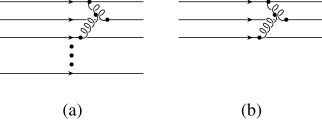
Figure 29: A baryon interaction and the corresponding connected component.

A connected piece that contains $n$ quark lines will be referred to as an $n$-body interaction. The colors on the outgoing quarks in an $n$-body interaction are a permutation of the colors on the incoming quarks, and the colors are distinct. Each outgoing line can be identified with an incoming line of the same color in a unique way. One can now relate connected graphs for baryons interactions with planar diagrams with a single quark loop. The leading in $N$ diagrams for the $n$-body interaction are given by taking a planar diagram with a single quark loop, cutting the loop in $n$ places, and setting the color on each cut line to equal the color of one of the incoming (or outgoing) quarks. For example, the interaction in fig. 29(b) is given by cutting fig. 10 once at each of the three fermion lines. Planar meson diagrams contain a single closed quark loop as the outer edge of the diagram. Baryon $n$-body graphs obtained from cutting the quark loop require that one twist the quark lines to orient them with their arrows pointing in the same direction, and do not necessarily look planar when drawn on a sheet of paper. For example, fig. 30 is a “planar” diagram for a two-body interaction. Baryon graphs in the double-line notation can have color index lines crossing each other due to the fermion line twists.

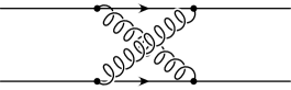
Figure 30: An example of a “planar” two-body baryon graph.

The relationship between meson and baryon graphs immediately gives us the $N$-counting rules for an $n$-body interaction in baryons: an $n$-body interaction is of order $N^{1-n}$, since planar quark diagrams are of order $N$, and $n$ index sums over quark colors have been eliminated by cutting $n$ fermion lines. Baryons contain $N$ quarks, so $n$-body interactions are equally important for any $n$. $n$-body interactions are of order $N^{1-n}$, but there are $\mathcal{O}(N^{n})$ ways of choosing $n$-quarks from a $N$-quark baryon. Thus the net effect of $n$-body interactions is of order $N$.

Diagrams with two disconnected pieces, such as fig. 31,

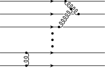
Figure 31: An example of a disconnected baryon interaction.

have a net effect of order $N^{2}$, those with three disconnected pieces are of order $N^{3}$, and so on. This is easy to understand. The baryon mass $M_{B}$ is of order $N$, since it contains $N$ quarks. The diagrams are an expansion of the baryon propagator, and sum to give

$$e^{-iM_{B}t}=1-iM_{B}t-{M_{B}^{2}t^{2}\over 2}+\ldots\ .$$

Diagrams with a single connected component produce the order $t$ term (the interaction can take place at any time) and are order $N\sim M_{B}$, those with two connected components give the order $t^{2}$ term (each connected component can take place at any time) and are order $N^{2}\sim M_{B}^{2}$, etc. Baryon interactions in the large $N$ limit are best studied in terms of connected diagrams, and the diagrammatic methods are the same as used in many-body theory.

Interactions of quarks in a baryon can be described by a non-relativistic Hamiltonian if the quarks are very heavy. The Hamiltonian has the form

$$H= Nm+\sum_{i}{p_{i}^{2}\over 2m}+{1\over N}\sum_{i\not=j}V\left(x_{i}-x_{j}\right)$$ (44)

$$+{1\over N^{2}}\sum_{i\not=j\not=k}V\left(x_{i}-x_{j},x_{i}-x_{k}\right)+\ldots.$$

Each term contributes $\mathcal{O}(N)$ to the total energy. The interaction terms in the Hamiltonian eq. (44) are the sum of many small contributions, so fluctuations are small, and each quark can be considered to move in an average background potential. Consequently, the Hartree approximation is exact in the large $N$ limit. The ground state wavefunction can be written as

$$\psi_{0}\left(x_{1},\ldots,x_{N}\right)=\prod_{i=1}^{N}\phi_{0}\left(x_{i}\right),$$

where $x_{i}$ are the positions of the quarks. The spatial wavefunction $\phi_{0}\left(x\right)$ is $N$-independent, so the baryon size is fixed in the $N\rightarrow\infty$ limit. The first excited state wavefunction is

$$\psi_{1}\left(x_{1},\ldots,x_{N}\right)={1\over\sqrt{N}}\sum_{k=1}^{N}\phi_{i}\left(x_{k}\right)\prod_{i=1,i\not=k}^{N}\phi_{0}\left(x_{i}\right).$$ (45)

Further details about this approach can be found in refs. [3, 5].

The $N$-counting rules can be extended to baryon matrix elements of color singlet operators. Consider a one-body operator, such as $\overline{q}q$. The baryon matrix element $\left\langle{B}\vphantom{\overline{q}qB}\right|{\overline{q}q}\left|\vphantom{B\overline{q}q}{B}\right\rangle$ has $N$ terms, since the operator can be inserted on any of the quark lines (see fig. 32(a)).

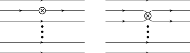
Figure 32: Baryon matrix elements of a one-body operator such as $\overline{q}q$, and a two-body operator such as $\overline{q}q\,\overline{q}q$.

The baryon matrix element is therefore $\leq\mathcal{O}(N)$. One obtains an inequality because there can be cancellations between the $N$ possible insertions. These cancellations will be crucial in unraveling the structure of baryons. Similarly, a two-body operator such as $\overline{q}q\,\overline{q}q$ has matrix element $\leq\mathcal{O}(N^{2})$, since there are $\mathcal{O}(N^{2})$ ways of inserting the operator in a baryon (see fig. 32(b)). In general, an $n$-body operator has matrix elements $\leq\mathcal{O}(N^{n})$.

The baryon-meson coupling constant is $\leq\sqrt{N}$. This can be seen from fig. 33,

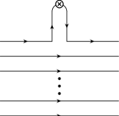
Figure 33: Diagrams for baryon-meson couplings.

which shows the matrix element of a fermion bilinear in a baryon. There are $N$ possible insertions of the fermion bilinear, so the matrix element is order $N$. The amplitude for a fermion bilinear to create a meson is the $Z$-factor, which is order $\sqrt{N}$, so the baryon-meson coupling constant is of order $N/Z=\sqrt{N}$. The baryon-meson scattering amplitude is $\leq\mathcal{O}(1)$. Two contributions to the scattering amplitude are shown in fig. 34.

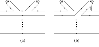
Figure 34: Diagrams for baryon-meson scattering.

Figure 34(a) has $N$ possible insertions of the fermion bilinear, and two meson $1/Z$-factors of $1/\sqrt{N}$ each, so the net amplitude is $\leq\mathcal{O}\left(1\right)$. The two bilinears must be inserted on the same quark line to conserve energy — the incoming meson injects energy into the quark line, which must be removed by the outgoing meson to give back the original baryon. If the bilinears are inserted on different quark lines, as in fig. 34(b), an additional gluon is needed to transfer energy between the two quark lines. The number of ways of choosing two quarks is $N^{2}$, the meson $1/Z$-factors are $1/\sqrt{N}$ each, and the two gluon couplings give $1/\sqrt{N}$ each, so the total amplitude is again $\leq\mathcal{O}(1)$. We have seen that the amplitudes $\rm baryon\rightarrow baryon+meson$ is of order $\sqrt{N}$, and $\rm baryon+meson\rightarrow baryon+meson$ is of order unity. One can similarly show that $\rm baryon+meson\rightarrow baryon+2\ mesons$ is of order $1/\sqrt{N}$, etc. As in purely mesonic amplitudes, each additional meson gives a factor of $1/\sqrt{N}$ suppression.

One can also look at the transition amplitudes for ground state baryon $+$ meson $\rightarrow$ excited baryon, or equivalently, for $B+M_{Q}\rightarrow B_{Q}$, where $M_{Q}$ and $B_{Q}$ are mesons and baryons containing a single heavy quark. In both processes, one of the quarks in the final state is different from the others. In the transition amplitude diagram, the meson amplitude must be inserted on the quark line that is different, as in fig. 35;

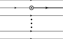
Figure 35: Diagrams for heavy meson + baryon $\rightarrow$ heavy baryon. The heavy quark is represented by a double line.

the meson operator either adds energy to the quark or converts it from a light quark to a heavy quark. Thus the combinatorial factor is unity, instead of $N$. The baryon with one excited (or heavy quark) has a wavefunction of the form eq. (45) in which one sums over the $N$ possible quarks which can be different, and multiplies by a normalization factor of $1/\sqrt{N}$. This produces an additional factor of $N\times 1/\sqrt{N}$, so the $B\rightarrow M+B^{*}$ amplitude is of order $\sqrt{N}$. This is $1/\sqrt{N}$ suppressed relative to the corresponding amplitude between ground state baryons.

Baryon-baryon scattering amplitudes at fixed velocity are of order $N$. It is important to study baryon scattering at fixed velocity, rather than fixed momentum, because the baryon mass is of order $N$. Working at fixed velocity avoids kinematic enhancements near threshold. The baryon-baryon scattering amplitude from diagrams such as fig. 36

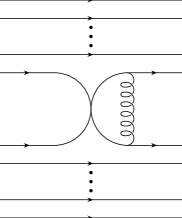
Figure 36: Baryon-baryon scattering.

has a combinatorial factor $N^{2}$ for the choice of two quarks, and $(1/\sqrt{N})^{2}$ for the two gluon couplings, for an overall factor of $N$. One could also consider a similar diagram without the exchanged gluon. Then the two quarks exchanged must have the same color, so the combinatorial factor is $N$. The net result is that the baryon-baryon scattering amplitude at fixed velocity is of order $N$. Baryon-baryon scattering can be described by classical trajectories in the large $N$ limit, since the particle masses are order $N$, and the scattering amplitude is also of order $N$.

The processes considered so far all have an $N$ dependence that is some power of $N$. There are also processes that are exponentially small in $N$, such as the cross-section for $e^{+}e^{-}\rightarrow B\overline{B}$. The amplitude to create a quark pair from the vacuum is some number $a<1$. The baryon has $N$ quarks, so the amplitude to create a $B\overline{B}$ pair is of order $a^{N}$, and is exponentially suppressed in $N$.

An important observation due to Witten is that all the $N$-counting rules mentioned above are the same as in a field theory with coupling constant $1/\sqrt{N}$, where the mesons are fundamental fields and the baryon is a soliton.

2 The Non-Relativistic Quark Model

The non-relativistic quark model treats the baryon as made of three non-relativistic quarks bound by a potential. The precise details of the potential will not be important for these lectures. All we need assume is that the ground state baryon is described by all three quarks in the same spatial wavefunction $\phi(x)$. The wavefunction must then be completely symmetric in spin and flavor. In the case of three flavors, there are six possible quark states $u\uparrow$, $u\downarrow$, $d\uparrow$, $d\downarrow$, $s\uparrow$, $s\downarrow$. The potential is assumed to be spin and flavor independent, so the non-relativistic quark model has an $SU(6)$ spin-flavor symmetry under which these six states transform as the fundamental representation. The ground state baryons transform as the completely symmetric product of three ${\bf 6}$’s of $SU(6)$, which is the $\bf 56$ dimensional representation.

Three spin $1/2$’s added together can give spin $1/2$ or spin $3/2$, so the baryon $\bf 56$ contains spin-1/2 and spin-3/2 baryons. The spin-$3/2$ wavefunction in the $m=3/2$ state is simple, it is $\uparrow\uparrow\uparrow$, and is completely symmetric. The flavor wavefunction must also be completely symmetric. It can have the form $uuu$, $(uud+udu+duu)/\sqrt{3}$, etc. The spin-3/2 baryons are the decuplet baryons, shown in fig. 37.

Figure 37: Flavor $SU(3)$ weight diagram for the decuplet baryons. The horizontal axis is $I_{3}$, and the vertical axis is hypercharge.

The spin-$1/2$ baryon wavefunctions are slightly more complicated. There are no spin-$1/2$ baryons in which all three quarks are the same, for then the wavefunction would be completely symmetric in flavor, thus completely symmetric in spin, and so spin-$3/2$. Consider a spin-$1/2$ baryon in which two of the quarks are identical, such as $uud$. The spin wavefunction for the two identical quarks must be completely symmetric, so the total spin wavefunction of the baryon in an $m=1/2$ state must have the form

$$\uparrow\uparrow\downarrow+\lambda(\uparrow\downarrow+\downarrow\uparrow)\uparrow.$$

The constant $\lambda=-1/2$ can be determined by requiring that the raising operator $J_{+}$ annihilates the state, since it is a $j=1/2$, $m=1/2$ state. Thus the wavefunction of the baryon can be written as

$${1\over\sqrt{6}}\,uud\,\left[2\uparrow\uparrow\downarrow-\uparrow\downarrow\uparrow-\downarrow\uparrow\uparrow\right].$$ (46)

Actually, one should add cyclic permutations (and divide by $1/\sqrt{3}$) to ensure that the wavefunction is completely symmetric. However, for most calculations, one can work just as well with eq. (46). We have determined the wavefunctions of six of the octet baryons. The remaining two states have three different quarks, $uds$. The $\Sigma^{0}$ is constructed using the combination $(uds+dus)/\sqrt{2}$. This symmetrizes the wavefunction in the first two flavors, and so one constructs the wavefunction as in eq. (46),

$${1\over\sqrt{12}}\,(uds+dus)\,\left[2\uparrow\uparrow\downarrow-\uparrow\downarrow\uparrow-\downarrow\uparrow\uparrow\right].$$

The $\Lambda$ state is constructed by antisymmetrizing $uds$ in the first two flavors, $(uds-dus)/\sqrt{2}$. The spin-wavefunction must also be antisymmetric in the first two flavors, so the $\Lambda$ wavefunction is

$${1\over 2}\,(uds-dus)\,\left[\uparrow\downarrow\uparrow-\downarrow\uparrow\uparrow\right],$$

which can be abbreviated to

$${1\over\sqrt{2}}\,uds\,\left[\uparrow\downarrow\uparrow-\downarrow\uparrow\uparrow\right].$$

The entire spin of the $\Lambda$ is carried by the $s$-quark. The spin-$1/2$ octet is shown in fig. 38. The spin-$1/2$ octet and spin-$3/2$ decuplet together make up the $\bf 56$ of $SU(6)$. The permutation symmetry properties of the baryons under spin $SU(2)$ and flavor $SU(3)$ are:

$${\bf 8}=\left(\raisebox{-0.5pt}{\hbox{\rule{0.4pt}{6.5pt}\hskip-0.4pt\rule{6.5pt}{0.4pt}\hskip-6.5pt\rule[6.5pt]{6.5pt}{0.4pt}}\rule[6.5pt]{0.4pt}{0.4pt}\hskip-0.4pt\rule{0.4pt}{6.5pt}},\ \raisebox{-3.5pt}{\hbox{\rule{0.4pt}{6.5pt}\hskip-0.4pt\rule{6.5pt}{0.4pt}\hskip-6.5pt\rule[6.5pt]{6.5pt}{0.4pt}}\rule[6.5pt]{0.4pt}{0.4pt}\hskip-0.4pt\rule{0.4pt}{6.5pt}}\hskip-6.9pt\raisebox{3.0pt}{\hbox{\rule{0.4pt}{6.5pt}\hskip-0.4pt\rule{6.5pt}{0.4pt}\hskip-6.5pt\rule[6.5pt]{6.5pt}{0.4pt}}\rule[6.5pt]{0.4pt}{0.4pt}\hskip-0.4pt\rule{0.4pt}{6.5pt}}\hskip-0.4pt\raisebox{3.0pt}{\hbox{\rule{0.4pt}{6.5pt}\hskip-0.4pt\rule{6.5pt}{0.4pt}\hskip-6.5pt\rule[6.5pt]{6.5pt}{0.4pt}}\rule[6.5pt]{0.4pt}{0.4pt}\hskip-0.4pt\rule{0.4pt}{6.5pt}}\right)\qquad{\bf 10}=\left(\raisebox{-0.5pt}{\hbox{\rule{0.4pt}{6.5pt}\hskip-0.4pt\rule{6.5pt}{0.4pt}\hskip-6.5pt\rule[6.5pt]{6.5pt}{0.4pt}}\rule[6.5pt]{0.4pt}{0.4pt}\hskip-0.4pt\rule{0.4pt}{6.5pt}}\hskip-0.4pt\raisebox{-0.5pt}{\hbox{\rule{0.4pt}{6.5pt}\hskip-0.4pt\rule{6.5pt}{0.4pt}\hskip-6.5pt\rule[6.5pt]{6.5pt}{0.4pt}}\rule[6.5pt]{0.4pt}{0.4pt}\hskip-0.4pt\rule{0.4pt}{6.5pt}}\hskip-0.4pt\raisebox{-0.5pt}{\hbox{\rule{0.4pt}{6.5pt}\hskip-0.4pt\rule{6.5pt}{0.4pt}\hskip-6.5pt\rule[6.5pt]{6.5pt}{0.4pt}}\rule[6.5pt]{0.4pt}{0.4pt}\hskip-0.4pt\rule{0.4pt}{6.5pt}},\ \raisebox{-0.5pt}{\hbox{\rule{0.4pt}{6.5pt}\hskip-0.4pt\rule{6.5pt}{0.4pt}\hskip-6.5pt\rule[6.5pt]{6.5pt}{0.4pt}}\rule[6.5pt]{0.4pt}{0.4pt}\hskip-0.4pt\rule{0.4pt}{6.5pt}}\hskip-0.4pt\raisebox{-0.5pt}{\hbox{\rule{0.4pt}{6.5pt}\hskip-0.4pt\rule{6.5pt}{0.4pt}\hskip-6.5pt\rule[6.5pt]{6.5pt}{0.4pt}}\rule[6.5pt]{0.4pt}{0.4pt}\hskip-0.4pt\rule{0.4pt}{6.5pt}}\hskip-0.4pt\raisebox{-0.5pt}{\hbox{\rule{0.4pt}{6.5pt}\hskip-0.4pt\rule{6.5pt}{0.4pt}\hskip-6.5pt\rule[6.5pt]{6.5pt}{0.4pt}}\rule[6.5pt]{0.4pt}{0.4pt}\hskip-0.4pt\rule{0.4pt}{6.5pt}}\right).$$

Figure 38: Flavor $SU(3)$ weight diagram for the baryon octet. The horizontal axis is $I_{3}$, and the vertical axis is hypercharge.

It is straightforward to compute baryon properties in the non-relativistic quark model. The axial coupling constant $g_{A}$ of the proton is given by the matrix element $\left\langle{p}\vphantom{\overline{q}\gamma^{\mu}\gamma_{5}\tau^{3}p}\right|{\overline{q}\gamma^{\mu}\gamma_{5}\tau^{3}}\left|\vphantom{p\overline{q}\gamma^{\mu}\gamma_{5}\tau^{3}}{p}\right\rangle$. In the non-relativistic limit, this reduces to the matrix element of $q^{\dagger}\sigma^{3}\tau^{3}q$, an operator which is $+1$ on $u\uparrow$ and $d\downarrow$, $-1$ on $u\downarrow$ and $d\uparrow$ and zero on strange quarks. The proton matrix element is

$$g_{A}={4\over 6}\left[1+1+1\right]+{1\over 6}\left[1-1-1\right]+{1\over 6}\left[-1+1-1\right]=\frac{5}{3},$$

where the first term is $(2/\sqrt{6})^{2}$ times the matrix elements for $u\uparrow$, $u\uparrow$, $d\downarrow$, etc. obtained using the wavefunction eq. (46).

Similarly, one can compute the magnetic moments of the baryons. The magnetic moment operator is $\mu\sigma^{3}$, where $\mu$ is the magnetic moment of the quark, and $\sigma^{3}$ is the spin operator. The quarks have magnetic moments $\mu_{u}$, $\mu_{d}$ and $\mu_{s}$. If the $u$ and $d$ quarks are degenerate in mass, $\mu_{u}=-2\mu_{d}$. The computation of the baryon magnetic moments in the non-relativistic quark model is left as an exercise.

One can repeat the entire non-relativistic quark model analysis for $N$ colors. It is convenient to choose $N=2m+1$, so that $N$ is always odd. The baryons form the completely symmetric tensor of $SU(6)$ with $N$ indices,

$$\raisebox{-0.5pt}{\hbox{\rule{0.4pt}{6.5pt}\hskip-0.4pt\rule{6.5pt}{0.4pt}\hskip-6.5pt\rule[6.5pt]{6.5pt}{0.4pt}}\rule[6.5pt]{0.4pt}{0.4pt}\hskip-0.4pt\rule{0.4pt}{6.5pt}}\hskip-0.4pt\raisebox{-0.5pt}{\hbox{\rule{0.4pt}{6.5pt}\hskip-0.4pt\rule{6.5pt}{0.4pt}\hskip-6.5pt\rule[6.5pt]{6.5pt}{0.4pt}}\rule[6.5pt]{0.4pt}{0.4pt}\hskip-0.4pt\rule{0.4pt}{6.5pt}}\hskip-0.4pt\raisebox{-0.5pt}{\hbox{\rule{0.4pt}{6.5pt}\hskip-0.4pt\rule{6.5pt}{0.4pt}\hskip-6.5pt\rule[6.5pt]{6.5pt}{0.4pt}}\rule[6.5pt]{0.4pt}{0.4pt}\hskip-0.4pt\rule{0.4pt}{6.5pt}}\cdots\raisebox{-0.5pt}{\hbox{\rule{0.4pt}{6.5pt}\hskip-0.4pt\rule{6.5pt}{0.4pt}\hskip-6.5pt\rule[6.5pt]{6.5pt}{0.4pt}}\rule[6.5pt]{0.4pt}{0.4pt}\hskip-0.4pt\rule{0.4pt}{6.5pt}}\hskip-0.4pt\raisebox{-0.5pt}{\hbox{\rule{0.4pt}{6.5pt}\hskip-0.4pt\rule{6.5pt}{0.4pt}\hskip-6.5pt\rule[6.5pt]{6.5pt}{0.4pt}}\rule[6.5pt]{0.4pt}{0.4pt}\hskip-0.4pt\rule{0.4pt}{6.5pt}}$$ (47)

This decomposes under $SU(2)_{\rm spin}\times SU(3)_{\rm flavor}$ as a tower of representations with $J=1/2$, $J=3/2$, …$J=N/2$,

$$\left(\frac{1}{2},\ \raisebox{-3.5pt}{\hbox{\rule{0.4pt}{6.5pt}\hskip-0.4pt\rule{6.5pt}{0.4pt}\hskip-6.5pt\rule[6.5pt]{6.5pt}{0.4pt}}\rule[6.5pt]{0.4pt}{0.4pt}\hskip-0.4pt\rule{0.4pt}{6.5pt}}\hskip-6.9pt\raisebox{3.0pt}{\hbox{\rule{0.4pt}{6.5pt}\hskip-0.4pt\rule{6.5pt}{0.4pt}\hskip-6.5pt\rule[6.5pt]{6.5pt}{0.4pt}}\rule[6.5pt]{0.4pt}{0.4pt}\hskip-0.4pt\rule{0.4pt}{6.5pt}}\hskip-0.4pt\raisebox{-3.5pt}{\hbox{\rule{0.4pt}{6.5pt}\hskip-0.4pt\rule{6.5pt}{0.4pt}\hskip-6.5pt\rule[6.5pt]{6.5pt}{0.4pt}}\rule[6.5pt]{0.4pt}{0.4pt}\hskip-0.4pt\rule{0.4pt}{6.5pt}}\hskip-6.9pt\raisebox{3.0pt}{\hbox{\rule{0.4pt}{6.5pt}\hskip-0.4pt\rule{6.5pt}{0.4pt}\hskip-6.5pt\rule[6.5pt]{6.5pt}{0.4pt}}\rule[6.5pt]{0.4pt}{0.4pt}\hskip-0.4pt\rule{0.4pt}{6.5pt}}\hskip-0.4pt\raisebox{-3.5pt}{\hbox{\rule{0.4pt}{6.5pt}\hskip-0.4pt\rule{6.5pt}{0.4pt}\hskip-6.5pt\rule[6.5pt]{6.5pt}{0.4pt}}\rule[6.5pt]{0.4pt}{0.4pt}\hskip-0.4pt\rule{0.4pt}{6.5pt}}\hskip-6.9pt\raisebox{3.0pt}{\hbox{\rule{0.4pt}{6.5pt}\hskip-0.4pt\rule{6.5pt}{0.4pt}\hskip-6.5pt\rule[6.5pt]{6.5pt}{0.4pt}}\rule[6.5pt]{0.4pt}{0.4pt}\hskip-0.4pt\rule{0.4pt}{6.5pt}}\cdots\raisebox{-3.5pt}{\hbox{\rule{0.4pt}{6.5pt}\hskip-0.4pt\rule{6.5pt}{0.4pt}\hskip-6.5pt\rule[6.5pt]{6.5pt}{0.4pt}}\rule[6.5pt]{0.4pt}{0.4pt}\hskip-0.4pt\rule{0.4pt}{6.5pt}}\hskip-6.9pt\raisebox{3.0pt}{\hbox{\rule{0.4pt}{6.5pt}\hskip-0.4pt\rule{6.5pt}{0.4pt}\hskip-6.5pt\rule[6.5pt]{6.5pt}{0.4pt}}\rule[6.5pt]{0.4pt}{0.4pt}\hskip-0.4pt\rule{0.4pt}{6.5pt}}\hskip-0.4pt\raisebox{3.0pt}{\hbox{\rule{0.4pt}{6.5pt}\hskip-0.4pt\rule{6.5pt}{0.4pt}\hskip-6.5pt\rule[6.5pt]{6.5pt}{0.4pt}}\rule[6.5pt]{0.4pt}{0.4pt}\hskip-0.4pt\rule{0.4pt}{6.5pt}}\right)\qquad\left(\frac{3}{2},\ \raisebox{-3.5pt}{\hbox{\rule{0.4pt}{6.5pt}\hskip-0.4pt\rule{6.5pt}{0.4pt}\hskip-6.5pt\rule[6.5pt]{6.5pt}{0.4pt}}\rule[6.5pt]{0.4pt}{0.4pt}\hskip-0.4pt\rule{0.4pt}{6.5pt}}\hskip-6.9pt\raisebox{3.0pt}{\hbox{\rule{0.4pt}{6.5pt}\hskip-0.4pt\rule{6.5pt}{0.4pt}\hskip-6.5pt\rule[6.5pt]{6.5pt}{0.4pt}}\rule[6.5pt]{0.4pt}{0.4pt}\hskip-0.4pt\rule{0.4pt}{6.5pt}}\hskip-0.4pt\raisebox{-3.5pt}{\hbox{\rule{0.4pt}{6.5pt}\hskip-0.4pt\rule{6.5pt}{0.4pt}\hskip-6.5pt\rule[6.5pt]{6.5pt}{0.4pt}}\rule[6.5pt]{0.4pt}{0.4pt}\hskip-0.4pt\rule{0.4pt}{6.5pt}}\hskip-6.9pt\raisebox{3.0pt}{\hbox{\rule{0.4pt}{6.5pt}\hskip-0.4pt\rule{6.5pt}{0.4pt}\hskip-6.5pt\rule[6.5pt]{6.5pt}{0.4pt}}\rule[6.5pt]{0.4pt}{0.4pt}\hskip-0.4pt\rule{0.4pt}{6.5pt}}\cdots\raisebox{-3.5pt}{\hbox{\rule{0.4pt}{6.5pt}\hskip-0.4pt\rule{6.5pt}{0.4pt}\hskip-6.5pt\rule[6.5pt]{6.5pt}{0.4pt}}\rule[6.5pt]{0.4pt}{0.4pt}\hskip-0.4pt\rule{0.4pt}{6.5pt}}\hskip-6.9pt\raisebox{3.0pt}{\hbox{\rule{0.4pt}{6.5pt}\hskip-0.4pt\rule{6.5pt}{0.4pt}\hskip-6.5pt\rule[6.5pt]{6.5pt}{0.4pt}}\rule[6.5pt]{0.4pt}{0.4pt}\hskip-0.4pt\rule{0.4pt}{6.5pt}}\hskip-0.4pt\raisebox{3.0pt}{\hbox{\rule{0.4pt}{6.5pt}\hskip-0.4pt\rule{6.5pt}{0.4pt}\hskip-6.5pt\rule[6.5pt]{6.5pt}{0.4pt}}\rule[6.5pt]{0.4pt}{0.4pt}\hskip-0.4pt\rule{0.4pt}{6.5pt}}\hskip-0.4pt\raisebox{3.0pt}{\hbox{\rule{0.4pt}{6.5pt}\hskip-0.4pt\rule{6.5pt}{0.4pt}\hskip-6.5pt\rule[6.5pt]{6.5pt}{0.4pt}}\rule[6.5pt]{0.4pt}{0.4pt}\hskip-0.4pt\rule{0.4pt}{6.5pt}}\hskip-0.4pt\raisebox{3.0pt}{\hbox{\rule{0.4pt}{6.5pt}\hskip-0.4pt\rule{6.5pt}{0.4pt}\hskip-6.5pt\rule[6.5pt]{6.5pt}{0.4pt}}\rule[6.5pt]{0.4pt}{0.4pt}\hskip-0.4pt\rule{0.4pt}{6.5pt}}\right)\cdots\left(\frac{N}{2},\ \raisebox{3.0pt}{\hbox{\rule{0.4pt}{6.5pt}\hskip-0.4pt\rule{6.5pt}{0.4pt}\hskip-6.5pt\rule[6.5pt]{6.5pt}{0.4pt}}\rule[6.5pt]{0.4pt}{0.4pt}\hskip-0.4pt\rule{0.4pt}{6.5pt}}\hskip-0.4pt\raisebox{3.0pt}{\hbox{\rule{0.4pt}{6.5pt}\hskip-0.4pt\rule{6.5pt}{0.4pt}\hskip-6.5pt\rule[6.5pt]{6.5pt}{0.4pt}}\rule[6.5pt]{0.4pt}{0.4pt}\hskip-0.4pt\rule{0.4pt}{6.5pt}}\hskip-0.4pt\raisebox{3.0pt}{\hbox{\rule{0.4pt}{6.5pt}\hskip-0.4pt\rule{6.5pt}{0.4pt}\hskip-6.5pt\rule[6.5pt]{6.5pt}{0.4pt}}\rule[6.5pt]{0.4pt}{0.4pt}\hskip-0.4pt\rule{0.4pt}{6.5pt}}\cdots\raisebox{3.0pt}{\hbox{\rule{0.4pt}{6.5pt}\hskip-0.4pt\rule{6.5pt}{0.4pt}\hskip-6.5pt\rule[6.5pt]{6.5pt}{0.4pt}}\rule[6.5pt]{0.4pt}{0.4pt}\hskip-0.4pt\rule{0.4pt}{6.5pt}}\hskip-0.4pt\raisebox{3.0pt}{\hbox{\rule{0.4pt}{6.5pt}\hskip-0.4pt\rule{6.5pt}{0.4pt}\hskip-6.5pt\rule[6.5pt]{6.5pt}{0.4pt}}\rule[6.5pt]{0.4pt}{0.4pt}\hskip-0.4pt\rule{0.4pt}{6.5pt}}\hskip-0.4pt\right)$$ (48)

The $SU(3)$ representations are complicated for arbitrary values of $N$. For example the $SU(3)$ weight diagram of the $J=1/2$ baryons is shown in fig. 39. The flavor representations simplify for two light flavors, where the states are $I=J=1/2$, …$I=J=N/2$.

Figure 39: Flavor $SU(3)$ weight diagram for the spin-1/2 baryons for $N$ colors. The numbers represent the degeneracy of each weight. The long edge of the diagram has $(N+1)/2$ states.

Baryon transformation properties under spin and flavor are $N$ dependent for $N_{F}\geq 3$, unlike for mesons. To apply the $1/N$ expansion to baryons it is convenient to make some identification between the arbitrary $N$ baryons and the $N=3$ baryons. The proton state for arbitrary $N$ will be taken to be the strangeness zero $I=J=1/2$ state. It contains $(m+1)$ $u$ quarks and $m$ $d$ quarks. The spin $J_{u}$ of the $u$ quarks must be $(m+1)/2$, since the spin wavefunction has to be completely symmetric. Similarly, the spin $J_{d}$ of the $d$ quarks must be $m/2$. The proton is then the $J=1/2$ state made by combining $J_{u}$ and $J_{d}$ to form spin-1/2. This is sufficient information to compute many of the proton properties as a function of $N$ [31]. For example, one can compute $g_{A}$, which is the matrix element of $\sigma^{3}\tau^{3}=2\left(J_{u}^{3}-J_{d}^{3}\right)$. By the Wigner-Eckart theorem

$$\left\langle{p}\vphantom{{\mathbf{J}}_{u}p}\right|{{\mathbf{J}}_{u}}\left|\vphantom{p{\mathbf{J}}_{u}}{p}\right\rangle=\lambda_{u}\left\langle{p}\vphantom{{\mathbf{J}}p}\right|{{\mathbf{J}}}\left|\vphantom{p{\mathbf{J}}}{p}\right\rangle,$$

$$\left\langle{p}\vphantom{{\mathbf{J}}_{d}p}\right|{{\mathbf{J}}_{d}}\left|\vphantom{p{\mathbf{J}}_{d}}{p}\right\rangle=\lambda_{d}\left\langle{p}\vphantom{{\mathbf{J}}p}\right|{{\mathbf{J}}}\left|\vphantom{p{\mathbf{J}}}{p}\right\rangle,$$

so that

$$\lambda_{u}={{\mathbf{J}}\cdot{\mathbf{J}}_{u}\over{\mathbf{J}}^{2}},\qquad\lambda_{d}={{\mathbf{J}}\cdot{\mathbf{J}}_{d}\over{\mathbf{J}}^{2}}.$$

Using ${\mathbf{J}}={\mathbf{J}}_{u}+{\mathbf{J}}_{d}$, one finds that

$$2{\mathbf{J}}\cdot{\mathbf{J}}_{u}={\mathbf{J}}^{2}+{\mathbf{J}}_{u}^{2}-{\mathbf{J}}_{d}^{2},\qquad 2{\mathbf{J}}\cdot{\mathbf{J}}_{d}={\mathbf{J}}^{2}+{\mathbf{J}}_{d}^{2}-{\mathbf{J}}_{u}^{2},$$

so that

$$\lambda_{u}={N+5\over 6},\qquad\lambda_{d}=-{N-1\over 6}.$$

In the large $N$ proton, $u$-quarks tend to have spin up, and $d$-quarks tend to have spin down. The axial coupling is

$$g_{A}=\lambda_{u}-\lambda_{d}={N+2\over 3},$$

which reduces to $5/3$ when $N=3$. $g_{A}\sim\mathcal{O}(N)$ in the large $N$ limit, which is consistent with the $N$-counting rules for the matrix element of a one-quark operator.

Problem 5.1 (Baryon Magnetic Moments)

Show the following:

1. The magnetic moment of a spin-$1/2$ baryon $q_{a}q_{a}q_{b}$ with two identical quarks is $4\mu_{a}/3-\mu_{b}/3$

2. The magnetic moment of the $\Lambda$ is $\mu_{s}$

3. The magnetic moment of the $\Sigma^{0}$ is the average of the $\Sigma^{+}$ and $\Sigma^{-}$ magnetic moments.

4. The magnetic moments of the spin-$3/2$ baryons is the sum of the moments of the constituent quarks.

5. Find the $\Delta^{+}\rightarrow p\gamma$ transition magnetic moment.

6 Spin-Flavor Symmetry for Baryons

1 Consistency Conditions

The large $N$ counting rules for baryons imply some highly non-trivial constraints among baryon couplings. The simplest to derive are relations among pion-baryon couplings, or equivalently, baryon axial current matrix elements. Related results also hold for $\rho$-baryon couplings, etc. and are discussed later. To derive the axial current relations, consider pion-nucleon scattering at fixed energy in the $N\rightarrow\infty$ limit. The argument is simplest in the chiral limit where the pion is massless, but this assumption is not necessary. The two assumptions required are that the baryon mass and $g_{A}$ are both of order $N$. One expects the baryon mass to be proportional to $N$, since it contains $N$ quarks. We have seen that the $N$-counting rules imply that $g_{A}$ is order $N$, unless there is a cancellation among the leading terms. In the non-relativistic quark model, $g_{A}=(N+2)/3$, so such a cancellation does not occur. It is reasonable that $g_{A}$ is of order $N$ in QCD, even though it need not have the value $(N+2)/3$.

The pion-nucleon vertex is

$${\partial_{\mu}\pi^{a}\over f}\left\langle{B}\vphantom{\overline{q}\gamma^{\mu}\gamma_{5}T^{a}qB}\right|{\overline{q}\gamma^{\mu}\gamma_{5}T^{a}q}\left|\vphantom{B\overline{q}\gamma^{\mu}\gamma_{5}T^{a}q}{B}\right\rangle,$$

and is of order $\sqrt{N}$, since $g_{A}\sim N$ and $f_{\pi}\sim\sqrt{N}$. Recoil effects are of order $1/N$, since the baryon mass is order $N$ and the pion energy is order one, and can be neglected. This allows one to simplify the expression for the nucleon axial current. The time component of the axial current between two nucleons at rest vanishes. The space components of the axial current between nucleons at rest can be written as

$$\left\langle B\right|\overline{\psi}\gamma^{i}\gamma_{5}T^{a}\psi\left|B\right\rangle=gN\left\langle B\right|X^{ia}\left|B\right\rangle,$$ (49)

where $\left\langle B\right|X^{ia}\left|B\right\rangle$ and $g$ are of order one. The coupling constant $g$ has been factored out so that the normalization of $X^{ia}$ can be chosen to simplify future expressions. $X^{ia}$ is an operator (or $4\times 4$ matrix) defined on nucleon states $p\uparrow$, $p\downarrow$, $n\uparrow$, $n\downarrow$, and $X^{ia}$ has a finite $N\rightarrow\infty$ limit.

The leading contribution to pion-nucleon scattering is from the pole graphs in fig. 40,

Figure 40: Pion-nucleon scattering diagrams of order $E$. The third diagram is $1/N^{2}$ suppressed in the large $N$ limit.

which contribute at order $E$ provided the intermediate state is degenerate with the initial and final states. Otherwise, the pole graph contribution is of order $E^{2}$. In the large $N$ limit, the pole graphs are of order $N$, since each pion-nucleon vertex is of order $\sqrt{N}$. There is also a direct two-pion-nucleon coupling that contributes at order $E$, which is of order $1/N$ in the large $N$ limit and can be neglected.

The pion-nucleon scattering amplitude for $\pi^{a}(q)+B(k)\rightarrow\pi^{b}(q^{\prime})+B(k^{\prime})$ from the pole graphs is

$$-i\ q^{i}q^{\prime\,j}{N^{2}g^{2}\over f_{\pi}^{2}}\left[{1\over q^{0}}X^{jb}X^{ia}-{1\over q^{\prime\,0}}X^{ia}X^{jb}\right],$$ (50)

where the amplitude is written in matrix form, with the matrix labels denoting the spin and flavor quantum numbers of the initial and final nucleons. Both initial and final nucleons are on-shell, so $q^{0}=q^{\prime\,0}$. The product of the $X$ matrices in eq. (50) sums over the possible spins and isospins of the intermediate nucleon. Since $f_{\pi}\sim\sqrt{N}$, the overall amplitude is of order $N$, which violates unitarity at fixed energy, and also contradicts the large $N$ counting rules of Witten. Thus large $N$ QCD with a $I=J=1/2$ nucleon multiplet interacting with a pion is an inconsistent field theory. There must be other states that cancel the order $N$ amplitude in eq. (50) so that the total amplitude is order one, consistent with unitarity. One can then generalize $X^{ia}$ to be an operator on this degenerate set of baryon states, with matrix elements equal to the corresponding axial current matrix elements. With this generalization, the form of eq. (50) is unchanged, and we obtain the first consistency condition for baryons [32],

$$\left[X^{ia},X^{jb}\right]=0\ .$$ (51)

This consistency condition implies that the baryon axial currents are represented by a set of operators $X^{ia}$ which commute in the large $N$ limit, a result also derived by Gervais and Sakita. [33]. There are additional commutation relations,

$$\left[J^{i},X^{jb}\right] = i\,\epsilon_{ijk}\,X^{kb},$$ (52)

$$\left[T^{a},X^{jb}\right] = i\,f_{abc}\,X^{jc},$$

since $X^{ia}$ has spin one and isospin one.

The algebra in eqs. (51) and (52) is a contracted $SU(2N_{F})$ algebra, where $N_{F}$ is the number of quark flavors. To see this, consider the algebra of operators in the non-relativistic quark model, which has an $SU(2N_{F})$ symmetry. The operators are

$$J^{i}=q^{\dagger}{\sigma^{i}\over 2}q,\ \ T^{a}=q^{\dagger}{T^{a}}q,\ \ G^{ia}=q^{\dagger}{\sigma^{i}\over 2}T^{a}q,$$

where $J^{i}$ is the spin, $T^{a}$ is the flavor generator, and $G^{ia}$ are the spin-flavor generators. The commutation relations involving $G^{ia}$ are

$$\left[G^{ia},G^{jb}\right] = \frac{i}{2N_{F}}\,\epsilon_{ijk}\delta_{ab}\,J^{k}+\frac{i}{4}\,f_{abc}\delta_{ij}\,T^{c}+\frac{i}{2}\,\epsilon_{ijk}d_{abc}\,G^{kc},$$

$$\left[J^{i},G^{jb}\right] = i\,\epsilon_{ijk}\,G^{kb},$$

$$\left[T^{a},G^{ib}\right] = i\,f_{abc}\,G^{jc}.$$ (53)

The algebra for large $N$ baryons in QCD is given by taking the limit

$$X^{ia}\equiv\lim_{N\rightarrow\infty}{G^{ia}\over N}.$$ (54)

The $SU(2N_{F})$ commutation relations eq. (53) turn into the commutation relations eqs. (51–52) in the large $N$ limit. The limiting process eq. (54) is known as a Lie algebra contraction.

We have just proved that the large $N$ limit of QCD has a contracted $SU(2N_{F})$ symmetry in the baryon sector. The unitary irreducible representations of the contracted Lie algebra can be obtained using the theory of induced representations, and can be shown to be infinite dimensional. The simplest irreducible representation for two flavors is a tower of states with $I=J=1/2,3/2$, etc. which is the set of states of the Skyrme model, or the large $N$ non-relativistic quark model. The irreducible representations for three flavors are more complicated. The $1/N$ expansion allows one to compute baryonic quantities using $SU(2N_{F})$ symmetry in the $N\rightarrow\infty$ limit. The $1/N$ corrections allow one to systematically study the form of $SU(2N_{F})$ symmetry breaking at finite $N$.

The pion-baryon coupling matrix $X^{ia}$ can be completely determined (up to an overall normalization $g$), since it is a generator of the $SU(2N_{F})_{c}$ algebra. It is easy to show that the large $N$ QCD predictions for the pion-baryon coupling ratios are the same as those obtained in the Skyrme model or non-relativistic quark model [34] in the $N\rightarrow\infty$ limit, because both these models also have a contracted $SU(2N_{F})$ symmetry in this limit. In the Skyrme model, the axial current in the $N\rightarrow\infty$ limit is $X^{ia}\propto\Tr AT^{i}A^{-1}T^{a}$, where $A$ is the Skyrmion collective coordinate. The $X$’s commute (and so form part of an $SU(2N_{F})_{c}$ algebra), since $A$ is a $c$-number. We have already seen how the quark model algebra reduces to $SU(2N_{F})_{c}$ in the large $N$ limit. While we have shown that $SU(2N_{F})_{c}$ is a symmetry of QCD in the large $N$ limit, we have not shown that $SU(2N_{F})$ is a symmetry of QCD for finite $N$. There is no reason to believe this is the case, so the $SU(2N_{F})$ symmetry of the quark model is not a symmetry of QCD. Nevertheless, many results obtained in the quark model will be rederived in QCD using the $SU(2N_{F})_{c}$ symmetry that is exact when $N\rightarrow\infty$.

It is useful to have an explicit representation of the $N\rightarrow\infty$ $SU(2N_{F})_{c}$ algebra to compute baryon properties in the $1/N$ expansion. There are two natural choices discussed above, the quark model (acting on $N$ quark baryons), or the Skyrme model. The two give equivalent results for physical quantities. An operator $O$ (such as $X^{ia}$) in the quark representation can be written as a $1/N$ expansion of Skyrme operators, and vice-versa,

$$O_{\rm quark}=O_{\rm Skyrme}^{(0)}+{1\over N}O_{\rm Skyrme}^{(1)}+\ldots.$$ (55)

A typical expression for a physical quantity is

$$a_{0}O_{0}+{a_{1}\over N}O_{1}+{a_{2}\over N^{2}}O_{2}+\ldots$$

where $a_{i}$ are coefficients, and $O_{i}$ are operators (such as $X^{ia}$ or $J^{i}$, etc.) in either the quark or Skyrme representation. The coefficients $a_{i}$ are not the same in the two representations, and the relation eq. (55) can be used to relate them. Clearly, any difference between the representations is of higher order in $1/N$ than the terms retained in the calculation. This is similar to the scheme dependence of physical quantities in Feynman diagram perturbation theory.

The $1/N$ expansion provides some deep connections between the quark model, the Skyrme model, and QCD. I do not have time in these lectures to discuss both the quark and Skyrme models, and the connection between them. Some of these results can be found in refs. [34, 35, 36]. In the rest of these lectures, I will compare the large $N$ results mostly with the quark model.

Problem 6.1 ($SU(2N_{F})$ Commutation Relations)

Derive the $SU(2N_{F})$ commutation relations eq. (53) using the quark operator relation $\left[q,q^{\dagger}\right]=1$.

2 $1/N$ Corrections

What makes the $1/N$ expansion for baryons interesting is that it is possible to compute $1/N$ corrections. This allows one to compute results for the physically relevant case $N=3$, rather than for the strict $N=\infty$ limit, which is only of formal interest.

The $1/N$ corrections to the axial couplings $X^{ia}$ are determined by considering the scattering process $\pi^{a}+B\rightarrow\pi^{b}+\pi^{c}+B$ at low energies. The baryon pole graphs that contribute in the large $N$ limit are shown in fig. 41.

Figure 41: The leading contribution to $\pi N\rightarrow\pi\pi N$ in the large $N$ and chiral limits.

The axial coupling $X^{ia}$ can be expanded in a series in $1/N$,

$$X^{ia}=X^{ia}_{0}+{1\over N}X^{ia}_{1}+\ldots,$$ (56)

where $X^{ia}_{0}$ satisfies eq. (51). An explicit calculation shows that the amplitude for pion-nucleon scattering from the diagrams in fig. 40 is proportional to

$$N^{3/2}\left[X^{ia},\left[X^{jb},X^{kc}\right]\right]$$

times kinematic factors, and violates unitarity unless the double commutator vanishes at least as fast as $N^{-3/2}$, so that the amplitude is at most of order one. In fact, one expects that the double commutator is of order $1/N^{2}$ from the large $N$ counting rule that the amplitude is order $1/\sqrt{N}$. Substituting eq. (56) into the constraint gives the consistency condition

$$\left[X^{ia}_{0},\left[X_{1}^{jb},X^{kc}_{0}\right]\right]+\left[X^{ia}_{0},\left[X^{jb}_{0},X_{1}^{kc}\right]\right]=0,$$ (57)

using $\left[X^{ia}_{0},X^{jb}_{0}\right]=0$ from eq. (51). For two flavors, the only solution to eq. (57) is that $X_{1}^{ia}$ is proportional to $X_{0}^{ia}$ [32]. This can be verified by an explicit computation of $X_{1}^{ia}$ as shown in section 8 [32, 35]. In the rest of this section, I will state the solutions of the various large $N$ consistency conditions. The solutions can be obtained using the methods discussed in detail in section 3.

At order $1/N$, the baryons in an irreducible representation of the contracted $SU(2N_{F})$ Lie algebra are no longer degenerate, but are split by an order $1/N$ mass term $\Delta M$. The intermediate baryon propagator in eq. (50) should be replaced by $1/(E-\Delta M)$. The energy $E$ of the pion is order one, whereas $\Delta M$ is of order $1/N$, so the propagator can be expanded to order $1/N$ as

$${1\over E-\Delta M}={1\over E}+{\Delta M\over E^{2}}+\ldots\ \ .$$ (58)

Including the $1/N$ corrections to the propagator does not affect the derivation of eq. (51), as the two terms in eq. (58) have different energy dependences. The first term leads to the consistency condition eq. (51) and the second gives the consistency condition on the baryon masses [37, 35],

$$\left[X^{ia},\left[X^{jb},\left[X^{kc},\Delta M\right]\right]\right]=0.$$ (59)

This constraint can be used to obtain the $1/N$ corrections to the baryon masses. The constraint eq. (59) is equivalent to a simpler constraint obtained by Jenkins using chiral perturbation theory [37]

$$\left[X^{ia},\left[X^{ia},\Delta M\right]\right]={\rm constant}.$$ (60)

The solution of eq. (59) or (60) is that the baryon mass splitting $\Delta M$ must be proportional to $J^{2}/N=j(j+1)/N$, where $j$ is the spin of the baryon [37]. This is precisely the form of the baryon mass splitting in the Skyrme model [38] or non-relativistic quark model.

The structure of the $1/N$ corrections shows that the expansion parameter is $J/N$, where $J$ is the spin of the baryon. For example, the baryon mass spectrum including the $J^{2}/N$ mass splitting has the form shown in fig. 42. The correction terms are only small near the bottom of the (infinite) baryon tower. For this reason, the $1/N$ expansion will only be considered for baryons with spin $J$ held fixed as $N\rightarrow\infty$.

Figure 42: The baryon mass spectrum including the $J^{2}/N$ term. The top of the tower is $j=N/2$, and the bottom is $j=1/2$.

3 Solution of Consistency Conditions

The solution of the large $N$ consistency conditions is the key to understanding the structure of baryons. The answer can be given quite simply [35, 36, 39, 40]. A quantity $Q$ that is of order $N^{r}$ in the large $N$ limit can be expanded in terms of the basic operators of the quark representation, $G^{ia}$, $J^{i}$ and $T^{a}$ as

$${Q\over N^{r}}={\mathcal{P}}\left({G^{ia}\over N},{J^{i}\over N},{T^{a}\over N}\right),$$ (61)

where $\mathcal{P}$ is a polynomial in its arguments, with coefficients that have an expansion in $1/N$. For example, we will soon see that the baryon mass in the flavor limit has the expansion

$${M_{B}\over N}=\left[a_{0}+a_{1}\left({J\over N}\right)^{2}+a_{2}\left({J\over N}\right)^{4}+\ldots\right],$$ (62)

where the $a_{i}(1/N)$ are unknown expansion coefficients. It is important to remember that no assumption is being made about the validity of the non-relativistic quark model. The operators $G^{ia}$, $J^{i}$ and $T^{a}$ are used as a way to do the $SU(2N_{F})$ group-theoretic computations. The expansion eq. (61) is true irrespective of the quark mass. For very heavy quarks, the non-relativistic Hartree picture is valid, and one can see that eq. (61) is consistent with the diagrammatic analysis of $1/N$ factors due to gluon exchange [39, 40]. Two-body operators on the right-hand side of eq. (61) are generated by an insertion of a one-body operator plus one-gluon exchange, three-body operators by a one-body operator plus two gluon exchanges, and so on, as shown in fig. 43. Each gluon exchange brings with it a factor of $1/N$ from the two couplings, which reproduces the $N$-counting in eq. (61). What is non-trivial is that the $N$-counting rules also hold if the quarks are massless.

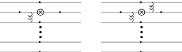
Figure 43: Two-body and three-body operator contributions to the baryon matrix elements of a QCD operator.

At first sight, all terms in the expansion eq. (61) are equally important, since an $r$-body operator in the expansion of $\mathcal{P}$ has a coefficient of order $1/N^{r}$, and matrix elements of $r$-body operators are of order $N^{r}$. Including all terms in eq. (61) is equivalent to saying that all possible $SU(2N_{F})$ representations are equally important, so that there is no predictive power. There are operator identities which allow one to simplify the general expansion eq. (61), and drop certain terms as subleading in $1/N$. It is these identities which allow one to use the $1/N$ expansion to make non-trivial predictions for baryons in QCD. The complete set of operator identities was derived in ref. [36]. They are listed in Tables 2 and 3 for the case of three and two flavors, respectively.

Table 2: $SU(6)$ Identities. Some of the identities need to be projected onto a given spin or flavor channel, which is given in parentheses.

$2\left\{J^{i},J^{i}\right\}+3\left\{T^{a},T^{a}\right\}+12\left\{G^{ia},G^{ia}\right\}=5N\left(N+6\right)$
$d^{abc}\left\{G^{ia},G^{ib}\right\}+{2\over 3}\left\{J^{i},G^{ic}\right\}+{1\over 4}d^{abc}\left\{T^{a},T^{b}\right\}={2\over 3}\left(N+3\right)T^{c}$
$\left\{T^{a},G^{ia}\right\}={2\over 3}\left(N+3\right)\ J^{i}$
${1\over 3}\left\{J^{k},T^{c}\right\}+d^{abc}\left\{T^{a},G^{kb}\right\}-\epsilon^{ijk}f^{abc}\left\{G^{ia},G^{jb}\right\}={4\over 3}\left(N+3\right)G^{kc}$
$-12\ \left\{G^{ia},G^{ia}\right\}+27\ \left\{T^{a},T^{a}\right\}-32\ \left\{J^{i},J^{i}\right\}=0$
$d^{abc}\ \left\{G^{ia},G^{ib}\right\}+{9\over 4}\ d^{abc}\ \left\{T^{a},T^{b}\right\}-{10\over 3}\ \left\{J^{i},G^{ic}\right\}=0$
$4\ \left\{G^{ia},G^{ib}\right\}=\left\{T^{a},T^{b}\right\}$	$({\bf 27})$
$\epsilon^{ijk}\ \left\{J^{i},G^{jc}\right\}=f^{abc}\ \left\{T^{a},G^{kb}\right\}$
$3\ d^{abc}\ \left\{T^{a},G^{kb}\right\}=\left\{J^{k},T^{c}\right\}-\epsilon^{ijk}f^{abc}\ \left\{G^{ia},G^{jb}\right\}$
$\epsilon^{ijk}\ \left\{G^{ia},G^{jb}\right\}=f^{acg}d^{bch}\ \left\{T^{g},G^{kh}\right\}$	$(\overline{\bf 10}+{\bf 10})$
$3\ \left\{G^{ia},G^{ja}\right\}=\left\{J^{i},J^{j}\right\}$	$(J=2)$
$3\ d^{abc}\ \left\{G^{ia},G^{jb}\right\}=\left\{J^{i},G^{jc}\right\}$	$(J=2)$

Table 3: $SU(4)$ Identities. Some of the identities need to be projected onto a given spin or flavor channel, which is given in the second column. The last column gives the transformation properties of the identities under $SU(2)\times SU(2)$.

$\left\{J^{i},J^{i}\right\}+\left\{I^{a},I^{a}\right\}+4\ \left\{G^{ia},G^{ia}\right\}={3\over 2}N\left(N+4\right)$		$(0,0)$
$2\left\{J^{i},G^{ia}\right\}=\left(N+2\right)\ I^{a}$		$(0,1)$
$2\left\{I^{a},G^{ia}\right\}=\left(N+2\right)\ J^{i}$	$(1,0)$
${1\over 2}\ \left\{J^{k},I^{c}\right\}-\epsilon^{ijk}\epsilon^{abc}\left\{G^{ia},G^{jb}\right\}=\left(N+2\right)\ G^{kc}$		$(1,1)$
$\left\{I^{a},I^{a}\right\}-\left\{J^{i},J^{i}\right\}=0$	$(0,0)$
$4\ \left\{G^{ia},G^{ib}\right\}=\left\{I^{a},I^{b}\right\}$	$(I=2)$	$(0,2)$
$\epsilon^{ijk}\ \left\{J^{i},G^{jc}\right\}=\epsilon^{abc}\ \left\{I^{a},G^{kb}\right\}$		$(1,1)$
$4\ \left\{G^{ia},G^{ja}\right\}=\left\{J^{i},J^{j}\right\}$	$(J=2)$	$(2,0)$

The operator identities allow one to eliminate certain operator combinations in the general expansion eq. (61). For example, for three flavors,

$$\left\{T^{a},G^{ia}\right\}=\frac{2}{3}\left(N+3\right)J^{i}$$

can be used to rewrite the two-body operator on the left-hand side in terms of the one-body operator on the right-hand side. The two-body operator matrix element is of order $N^{2}$, and the one-body operator matrix element is of order $N$, which is consistent with the coefficient of proportionality being of order $N$. The operator identities have been written in terms of anticommutators, since they are hermitian, and since commutators can be simplified using the $SU(2N_{F})$ commutation relations eq. (53). A study of the identities leads to the following reduction rules:

• All operator products in which two flavor indices are contracted using $\delta^{ab}$, $d^{abc}$ or $f^{abc}$, or two spin indices on $G$’s are contracted using $\delta^{ij}$ or $\epsilon^{ijk}$ can be eliminated.

• All operators in which two spin or isospin indices are contracted with a $\delta$ or $\epsilon$-symbol can be eliminated, with the exception of $J^{2}$.

The inclusion of $J^{2}$, but not $I^{2}$, in the set of independent operators does not break the symmetry between spin and isospin, because of the identity $I^{2}=J^{2}$.

As an application of the operator reduction rule, consider the baryon masses in the $SU(3)$ symmetry limit. The general form of the baryon mass is given by eq. (61),

$${M\over N}=\mathcal{P}\left({G^{ia}\over N},{J^{i}\over N},{T^{a}\over N}\right),$$

where the terms in $\mathcal{P}$ must be spin-zero flavor singlets, since those are the quantum numbers of $M$. Thus all terms in $\mathcal{P}$ are obtained by contracting the spin and flavor indices on $G^{ia}$, $J^{i}$ and $T^{a}$ using spin and flavor invariant tensors, such as $\delta^{ab}$ or $f^{abc}$. The operator reduction rule tells us that all terms involving $T^{a}$ or $G^{ia}$ can be eliminated, so that one is left with an expansion in $J^{i}$. Rotational invariance implies that the expansion is in $J^{2}$, and so has the form eq. (62), and leads to the spectrum in fig. 42.

Equation (62) shows that the baryon expansion parameter is $J/N$. One can compute baryon properties in a systematic expansion in $1/N$ provided one looks at states with $J$ fixed as $N\rightarrow\infty$. Generically, $J$ is a one-body operator and can have matrix elements of order $N$. The $1/N$ expansion is only valid for states in which $J$ is of order unity, i.e. for states at the bottom of the baryon tower in fig. 42. In these states, there is a cancellation between the $N$ possible insertions of the one-body operator $J$ on the $N$ quark lines. Generically, matrix elements of $G^{ia}$ and $T^{a}$ are $\mathcal{O}\left(N\right)$, so that $G^{ia}/N$ and $T^{a}/N$ are $\mathcal{O}\left(1\right)$. In the case of two flavors, there is an additional simplification that $I^{a}$ is $\mathcal{O}\left(1\right)$, so that $I^{a}/N$ is $1/N$ suppressed.

Problem 6.2

Prove the identity

$$4J^{i}G^{ia}=(N+2)I^{a}$$

for two quark flavors.

Solution: It is convenient to write $G^{ia}=(1/4)\sum_{\alpha}\sigma^{i}_{\alpha}\tau^{a}_{\alpha}$, where the sum is over the different quark lines in the baryon, each of which has a different color. Then

$$8J^{i}G^{ia} = \sum_{\alpha\beta}\sigma^{i}_{\alpha}\sigma^{i}_{\beta}\tau^{a}_{\beta}$$

$$= \sum_{\alpha=\beta}\sigma^{i}_{\alpha}\sigma^{i}_{\beta}\tau^{a}_{\beta}+\sum_{\alpha\not=\beta}\sigma^{i}_{\alpha}\sigma^{i}_{\beta}\tau^{a}_{\beta}.$$

The term with $\alpha=\beta$ can be written as

$$\sum_{\alpha=\beta}\sigma^{i}_{\alpha}\sigma^{i}_{\alpha}\tau^{a}_{\beta} = 3\sum_{\alpha}\tau^{a}$$

$$= 6I^{a}.$$

The terms with $\alpha\not=\beta$ can be simplified using the identity

$$\left[\sigma^{i}_{\alpha}\right]^{a}_{b}\ \left[\sigma^{i}_{\beta}\right]^{c}_{d}=2\delta^{a}_{d}\delta^{c}_{b}-\delta^{a}_{b}\delta^{c}_{d}\equiv 2S_{\rm exch}(\alpha,\beta)-1$$

where $S_{\rm exch}(\alpha,\beta)$ is the spin-exchange operator that exchanges the spins of the two quarks, to give

$$\sum_{\alpha\not=\beta}\sigma^{i}_{\alpha}\sigma^{i}_{\beta}\tau^{a}_{\beta}=\sum_{\alpha\not=\beta}\left[2S_{\rm exch}(\alpha,\beta)-1\right]\tau^{a}_{\beta}$$

The final state baryon is completely symmetric in spin $\otimes$ flavor, so one can replace $S_{\rm exch}(\alpha,\beta)$ by the flavor exchange operator $F_{\rm exch}(\alpha,\beta)$. The identity

$$[\tau^{g}_{\alpha}]^{a}_{b}\ [\tau^{g}_{\beta}]^{c}_{d}=2\delta^{a}_{d}\delta^{c}_{b}-\delta^{a}_{b}\delta^{c}_{d}\equiv 2F_{\rm exch}(\alpha,\beta)-1$$

allows one to rewrite this as

$$\sum_{\alpha\not=\beta}\tau^{g}_{\alpha}\tau^{g}_{\beta}\tau^{a}_{\beta}.$$

Then

$$\tau^{g}_{\beta}\tau^{a}_{\beta}=\delta^{ga}_{\beta}+i\epsilon_{gah}\tau^{h}_{\beta}$$

implies that

$$\sum_{\alpha\not=\beta}\tau^{g}_{\alpha}\tau^{g}_{\beta}\tau^{a}_{\beta} = \tau^{g}_{\alpha}\left(\delta^{ga}_{\beta}+i\epsilon_{gah}\tau^{h}_{\beta}\right)$$

$$= \sum_{\alpha\not=\beta}\tau^{a}_{\alpha}+\sum_{\alpha,\beta}i\epsilon_{gah}\tau^{g}_{\alpha}\tau^{h}_{\beta}-\sum_{\alpha=\beta}i\epsilon_{gah}\tau^{g}_{\alpha}\tau^{h}_{\beta}$$

$$= (N-1)\sum_{\alpha}\tau^{a}_{\alpha}+i\epsilon_{gah}\sum_{\alpha}\tau^{g}_{\alpha}\sum_{\beta}\tau^{h}_{\beta}$$

$$\ \ -i\sum_{\alpha}\epsilon_{gah}\left(\delta^{gh}+i\epsilon_{ghr}\tau^{r}_{\alpha}\right)$$

$$= 2(N-1)I^{a}+4i\epsilon_{gah}I^{g}I^{h}+2\epsilon_{gah}\epsilon_{ghr}I^{r}$$

$$= 2(N-1)I^{a}+2i\epsilon_{gah}\left[I^{g},I^{h}\right]+2\epsilon_{gah}\epsilon_{ghr}I^{r}$$

$$= 2(N-1)I^{a}$$

Combining the pieces gives the desired identity. More examples of this kind can be found in refs. [36, 39, 40].

7 Masses with SU(3) Breaking

The baryon masses can be computed in a systematic expansion in powers of $1/N$ and $SU(3)$ breaking. I will use a simplified version of the analysis of Jenkins and Lebed [41], by neglecting isospin breaking. This example is discussed in detail, to show how the formalism we have developed can be applied.

There are eight isospin-averaged baryon masses for the $N$, $\Lambda$, $\Sigma$, $\Xi$, $\Delta$, $\Sigma^{*}$, $\Xi^{*}$ and $\Omega$. The general form of the $SU(3)$ singlet mass term has already been worked out in eq. (61). At first order in $SU(3)$ breaking, the baryon mass term transforms as an $SU(3)$ octet. The most general spin-zero $SU(3)$ octet is a polynomial in $J^{i}$, $T^{a}$ and $G^{ia}$ with one free flavor index set to $8$. All operators with contracted flavor indices can be eliminated using the operator reduction rule, so one is left with terms with a single $T^{8}$ or $G^{i8}$, and powers of $J^{i}$,

$$\epsilon b_{1}T^{8}+\epsilon b_{3}{J^{2}T^{8}\over N^{2}}+\epsilon b_{5}{J^{4}T^{8}\over N^{4}}+\ldots$$

$$+\epsilon b_{2}{J^{i}G^{i8}\over N}+\epsilon b_{4}{J^{2}J^{i}G^{i8}\over N^{3}}+\ldots$$ (63)

where $\epsilon$ is a measure of $SU(3)$ breaking. $SU(3)$ breaking is due to the strange quark mass $m_{s}$. Chiral perturbation theory shows that there are non-analytic contributions to the baryon mass, such as $m_{s}^{3/2}$ and $m_{s}^{2}\log m_{s}$. The structure of $SU(3)$ breaking as a function of $m_{s}$ is highly non-trivial, but goes beyond the scope of these introductory lectures. For the purposes of the analysis here, I will treat $\epsilon$ as a small parameter of order $SU(3)$ breaking.

At second order in $SU(3)$ breaking, one can get a tensor with two free flavor indices set to $8$, and at third order, with three free flavor indices set to $8$. One can work out the general form of these terms, as in eq. (63). Eventually, the matrix elements will be taken between baryons for $N=3$. For this reason, one can stop the expansion of the mass term at three-body operators, since a baryon for $N=3$ contains three quarks. Operators with more than three quarks can be written as a linear combination of operators with three or fewer quarks. One simple way to see this is to write operators in normal ordered form, with all $q^{\dagger}$’s to the left of the $q$’s. Then $r$-body operators with $r>3$ vanish on baryons containing three quarks.

The order $\epsilon^{2}$ terms up to three-body operators are

$$\epsilon^{2}c_{2}{T^{8}T^{8}\over N}+\epsilon^{2}c_{3}{T^{8}J^{i}G^{i8}\over N^{2}}$$ (64)

and the $\epsilon^{3}$ term is

$$\epsilon^{3}d_{3}{T^{8}T^{8}T^{8}\over N^{2}}.$$ (65)

Combining eqs. (61)–(65) and stopping at three-body operators gives the baryon mass formula

$$M = a_{0}+a_{1}{J^{2}\over N}+\epsilon b_{1}T^{8}+\epsilon b_{2}{J^{i}G^{i8}\over N}+\epsilon b_{3}{J^{2}T^{8}\over N^{2}}+\epsilon^{2}c_{2}{T^{8}T^{8}\over N}$$ (66)

$$+\epsilon^{2}c_{3}{T^{8}J^{i}G^{i8}\over N^{2}}+\epsilon^{3}d_{3}{T^{8}T^{8}T^{8}\over N^{2}},$$

which gives the eight baryon masses in terms of eight parameters. This must be the case, since the baryon masses are independent if one works to arbitrary order in $1/N$ and $\epsilon$. The non-trivial information contained in eq. (66) is the $\epsilon$ and $N$ dependence of the various terms. Equation (66) will be used to derive a hierarchy of baryon mass relations to a given order in $\epsilon$ and $1/N$. To obtain these relations, one needs the matrix element of eq. (66) between baryon states. The matrix element of

$$\sqrt{12}\ T^{8}=\left(\begin{array}[]{ccc}1\\ &1\\ &&-2\\ \end{array}\right)=\left(\begin{array}[]{ccc}1\\ &1\\ &&1\\ \end{array}\right)-\left(\begin{array}[]{ccc}0\\ &0\\ &&3\\ \end{array}\right)$$

is

$$T^{8}={1\over\sqrt{12}}\left(N-3N_{s}\right),$$ (67)

where $N_{s}$ is the number of strange quarks. The operator $G^{i8}$ is

$$G^{i8}={1\over\sqrt{12}}\left(J^{i}-3J_{s}^{i}\right),$$

where $J^{i}$ is the quark spin, and

$$J_{s}^{i}=q^{\dagger}{\sigma^{i}\over 2}\left(\begin{array}[]{ccc}0\\ &0\\ &&1\\ \end{array}\right)q$$

is the strange quark spin. This gives

$$J^{i}G^{i8}={1\over\sqrt{12}}\left(J^{2}-3J\cdot J_{s}\right).$$

The total spin of the baryon is $J=J_{ud}+J_{s}$, where $J_{ud}$ is the spin of the $u$- and $d$-quarks, and $J_{s}$ is the spin of the strange quarks. One can write $J^{2}-3J\cdot J_{s}=3J_{ud}^{2}-J^{2}-3J_{s}^{2}$, and then use the identity $J_{ud}^{2}=I^{2}$, where $I$ is the isospin, to obtain

$$J^{i}G^{i8}={1\over\sqrt{12}}\left(3I^{2}-J^{2}-3J_{s}^{2}\right).$$ (68)

All the baryons are eigenstates of $N_{s}$, $I^{2}$, $J^{2}$ and $J_{s}^{2}$, so the matrix element of eq. (66) can be computed simply using eqs. (67) and (68). The matrix elements are listed in Table 4.

Table 4: Matrix elements of the mass operators, eq. (66). The first section of the table lists the matrix elements of the basic operators $N$, $N_{s}$, $J^{2}$, $J_{s}^{2}$ and $I^{2}$. These are used to compute the matrix elements of the remaining operators using eqs. (67)–(68).

	$N$	$\Lambda$	$\Sigma$	$\Xi$	$\Delta$	$\Sigma^{*}$	$\Xi^{*}$	$\Omega$
$N$	$3$	$3$	$3$	$3$	$3$	$3$	$3$	$3$
$N_{s}$	$0$	$1$	$1$	$2$	$0$	$1$	$2$	$3$
$J^{2}$	$3/4$	$3/4$	$3/4$	$3/4$	$15/4$	$15/4$	$15/4$	$15/4$
$J_{s}^{2}$	$0$	$3/4$	$3/4$	$2$	$0$	$3/4$	$2$	$15/4$
$I^{2}$	$3/4$	$0$	$2$	$3/4$	$15/4$	$2$	$3/4$	$0$
$1$	$1$	$1$	$1$	$1$	$1$	$1$	$1$	$1$
$J^{2}$	$3/4$	$3/4$	$3/4$	$3/4$	$15/4$	$15/4$	$15/4$	$15/4$
$2\sqrt{3}T^{8}$	$3$	$0$	$0$	$-3$	$3$	$0$	$-3$	$-6$
$4\sqrt{3}J^{i}G^{i8}$	$3/2$	$-3$	$3$	$-9/2$	$15/2$	$0$	$-15/2$	$-15$
$2\sqrt{3}J^{2}T^{8}$	$9/4$	$0$	$0$	$-9/4$	$45/4$	$0$	$-45/4$	$-45/2$
$\left(2\sqrt{3}T^{8}\right)^{2}$	$9$	$0$	$0$	$9$	$9$	$0$	$9$	$36$
$24T^{8}J^{i}G^{i8}$	$9/2$	$0$	$0$	$27/2$	$45/2$	$0$	$45/2$	$90$
$\left(2\sqrt{3}T^{8}\right)^{3}$	$27$	$0$	$0$	$-27$	$27$	$0$	$-27$	$-216$

Combining eq. (66) and Table 4 gives the baryon masses

$$M=HA,$$ (69)

where

$$M=\left(\begin{array}[]{cccccccc}m_{N}&m_{\Lambda}&m_{\Sigma}&m_{\Xi}&m_{\Delta}&m_{\Sigma^{*}}&m_{\Xi^{*}}&m_{\Omega}\\ \end{array}\right),$$

is a row vector of baryon masses,

$$A=\left(\begin{array}[]{cccccccc}1&1&1&1&1&1&1&1\\ 3/4&3/4&3/4&3/4&15/4&15/4&15/4&15/4\\ 3&0&0&-3&3&0&-3&-6\\ 3/2&-3&3&-9/2&15/2&0&-15/2&-15\\ 9/4&0&0&-9/4&45/4&0&-45/4&-45/2\\ 9&0&0&9&9&0&9&36\\ 9/2&0&0&27/2&45/2&0&45/2&90\\ 27&0&0&-27&27&0&-27&-216\\ \end{array}\right)$$

is the array of matrix elements from Table 4, and

$$H = \left(\begin{array}[]{cccccccc}H_{1}&H_{2}&H_{3}&H_{4}&H_{5}&H_{6}&H_{7}&H_{8}\\ \end{array}\right)$$

$$= \left(\begin{array}[]{cccccccc}a_{0}&{a_{1}\over N}&{\epsilon b_{1}\over 2\sqrt{3}}&{\epsilon b_{2}\over 4\sqrt{3}N}&{\epsilon b_{3}\over 2\sqrt{3}N^{2}}&{\epsilon^{2}c_{2}\over 12N}&{\epsilon^{2}c_{3}\over 24N^{2}}&{\epsilon^{3}d_{3}\over 24\sqrt{3}N^{3}}\\ \end{array}\right)$$

is the row vector of coefficients.

The classification of the mass operators in powers of $1/N$ and $\epsilon$ is shown in Table 5.

Table 5: The order in $1/N$ and $\epsilon$ of the eight mass operators.

	$N$	$1$	$1/N$	$1/N^{2}$
$1$	$1$		$J^{2}$
$\epsilon$		$T^{8}$	$J^{i}G^{i8}$	$J^{2}T^{8}$
$\epsilon^{2}$			$T^{8}T^{8}$	$T^{8}J^{i}G^{i8}$
$\epsilon^{3}$				$T^{8}T^{8}T^{8}$

There are no relations if all the operators are retained in eq. (69). The most accurate relation is obtained if one omits the operator $T^{8}T^{8}T^{8}$ which contributes at order $\epsilon^{3}/N^{2}$. This gives a baryon mass relation that has an error of order $\epsilon^{3}/N^{2}$. The mass relation is obtained by writing eq. (69) as

$$H=MA^{-1}.$$ (72)

Omitting $T^{8}T^{8}T^{8}$ means that $H_{8}=0$, which gives the relation $R8$ (on multiplying by 162 to eliminate fractional coefficients)

$$(R8):\qquad\qquad\Delta-3\Sigma^{*}+3\Xi^{*}-\Omega=\mathcal{O}\left(\epsilon^{3}/N^{2}\right),$$ (73)

since $H_{8}$ is $\mathcal{O}\left(\epsilon^{3}/N^{2}\right)$. The next most accurate relation is obtained by dropping $T^{8}T^{8}T^{8}$ and $T^{8}J^{i}G^{i8}$. This is equivalent to $H_{8}=0$ and $H_{7}=0$ in eq. (72). The relation $H_{8}$ is eq. (73). The relation $H_{7}=0$ is

$$(R7):14N-21\Lambda-7\Sigma+14\Xi-8\Delta+10\Sigma^{*}-4\Xi^{*}-6\Omega=\mathcal{O}\left(\epsilon^{2}/N^{2}\right).$$

At the next step, one can drop either the $T^{8}T^{8}$ operator, which gives a new relation with an error $\mathcal{O}\left(\epsilon^{2}/N\right)$, or drop the $J^{2}T^{8}$ operator, which gives a relation with an error $\mathcal{O}\left(\epsilon/N^{2}\right)$. Dropping both gives no additional independent relation. One can then drop $J^{i}G^{i8}$ to get a $\mathcal{O}\left(\epsilon/N\right)$ relation, and then drop either $T^{8}$ or $J^{2}$ to get $\mathcal{O}\left(\epsilon\right)$ or $\mathcal{O}\left(1/N\right)$ relations.

This procedure gives a hierarchy of mass relations $H_{i}=0$. There are no free parameters in any of the relations, since all coefficients were fixed by group theory. It is convenient to write down relations that have definite $SU(6)$ and $SU(2)\times SU(3)$ transformation properties. These relations are orthogonal to each other, since different irreducible representations of a symmetry group are orthogonal. One can make the relations $H_{i}=0$ orthogonal using the Gram-Schmidt procedure starting with $H_{8}=0$ and working down to $H_{1}=0$, with respect to the metric (see problem 7.1)

$$g={\rm diag}\left(\begin{array}[]{cccccccc}\frac{1}{4}&\frac{1}{2}&\frac{1}{6}&\frac{1}{4}&\frac{1}{16}&\frac{1}{12}&\frac{1}{8}&\frac{1}{4}\end{array}\right).$$ (74)

The entries in this matrix are the reciprocals of the number of baryon states, e.g. there are four nucleon states, $p\uparrow$, $p\downarrow$, $n\uparrow$, $n\downarrow$, two $\Lambda$ states $\Lambda\uparrow$, $\Lambda\downarrow$, etc. The resulting relations are tabulated in Table 6.

Table 6: Baryon mass relations with the order in $\epsilon$ and $1/N$. The entries in the table are the coefficients of $m_{N}$, etc. in the eight relations. The fractional error computed using the experimental values for the masses is listed in the last column.

	$N$	$\Lambda$	$\Sigma$	$\Xi$	$\Delta$	$\Sigma^{*}$	$\Xi^{*}$	$\Omega$	Order	Frac. Error
$R1$	$2$	$1$	$3$	$2$	$8$	$6$	$4$	$2$	$N$
$R2$	$-10$	$-5$	$-15$	$-10$	$16$	$12$	$8$	$4$	$1/N$	$0.18$	$\pm$	$0.0004$
$R3$	$1$	$0$	$0$	$-1$	$4$	$0$	$-2$	$-2$	$\epsilon$	$0.27$	$\pm$	$0.0007$
$R4$	$-7$	$-2$	$6$	$3$	$4$	$0$	$-2$	$-2$	$\epsilon/N$	$0.052$	$\pm$	$0.0003$
$R5$	$-2$	$3$	$-9$	$8$	$4$	$0$	$-2$	$-2$	$\epsilon/N^{2}$	$0.011$	$\pm$	$0.0003$
$R6$	$2$	$-3$	$-1$	$2$	$16$	$-20$	$-8$	$12$	$\epsilon^{2}/N$	$0.0048$	$\pm$	$0.0004$
$R7$	$-14$	$21$	$7$	$-14$	$8$	$-10$	$-4$	$6$	$\epsilon^{2}/N^{2}$	$0.0017$	$\pm$	$0.0002$
$R8$	$0$	$0$	$0$	$0$	$1$	$-3$	$3$	$-1$	$\epsilon^{3}/N^{2}$	$0.0009$	$\pm$	$0.0003$

The mass relations can now be compared with experiment. The relations derived are homogeneous relations, and have no standard normalization, i.e. they can be multiplied by an arbitrary overall coefficient. It is therefore best to compute the fractional error on each relation. Relations which hold to higher order in $1/N$ or $\epsilon$ should work better, if $1/N$ and $\epsilon$ are good expansion parameters. The fractional error is defined using the following procedure. Each relation is written in the form $L=R$, where both sides are linear combinations of masses with positive coefficients. For example, the $\mathcal{O}\left(\epsilon^{3}/N^{2}\right)$ relation $R8$ is written as

$$L=\Delta+3\Xi^{*}=3\Sigma^{*}+\Omega=R.$$

One then computes the fractional accuracy of the relation, $\left|L-R\right|/\left(\left(L+R\right)/2\right)$ using the experimental values for the isospin averaged baryon masses (in MeV),

$$\kern-15.00002pt\begin{array}[]{cccccccc}m_{N}&m_{\Lambda}&m_{\Sigma}&m_{\Xi}\\ 938.91897\pm 0.0002&1115.684\pm 0.006&1193.12\pm 0.04&1318.11\pm 0.31\\ \\ m_{\Delta}&m_{\Sigma^{*}}&m_{\Xi^{*}}&m_{\Omega}\\ 1231.3\pm 1.1&1384.6\pm 0.4&1533.4\pm 0.3&1672.45\pm 0.29\end{array}.$$

Since the baryon mass is of order $N$, the fractional accuracy of $R8$ is $\mathcal{O}\left(\epsilon^{3}/N^{3}\right)$, since the denominator is order $N$. The fractional accuracy of the baryon mass relations is listed in Table 6 and plotted in fig. 44.

Figure 44: Accuracy of the large $N$ baryon mass relations from Table 6. The error bars are those on the experimentally measured baryon masses. The shape of the points gives their order in $SU(3)$ breaking: $\bigcirc$ is $\mathcal{O}\left(1\right)$, $\blacktriangle$ is $\mathcal{O}\left(\epsilon\right)$, $\Box$ is $\mathcal{O}\left(\epsilon^{2}\right)$, and $\times$ is $\mathcal{O}\left(\epsilon^{3}\right)$. The differences within the $\mathcal{O}\left(\epsilon\right)$ and $\mathcal{O}\left(\epsilon^{2}\right)$ relations are explained by including the factors of $1/N$. The accuracies of the baryon mass relations are $1/N^{2}$, $\epsilon/N$, $\epsilon/N^{2}$, $\epsilon/N^{3}$, $\epsilon^{2}/N^{2}$, $\epsilon^{2}/N^{3}$ and $\epsilon^{3}/N^{3}$, respectively.

The error bars on the points are from the experimental errors on the measured baryon masses. The points in fig. 44 have been plotted so that relations of the same order in $\epsilon$ have the same symbol. The standard $SU(3)$ analysis of baryon masses which might be familiar to some of you is equivalent to using the relations we have derived, but ignoring the powers of $N$. The Gell-Mann–Okubo formula for the baryon octet, and the equal spacing rule for the baryon decuplet are linear combinations of the two $\epsilon^{2}$ relations and one $\epsilon^{3}$ relation we have obtained. Clearly, $SU(3)$ breaking alone is not the whole story, and including the factors of $1/N$ provides a much better understanding of the data than $SU(3)$ alone. It is obvious from the figure that the $1/N$ and $\epsilon$ expansions explain the observed data. There is also clear evidence for the validity of the $1/N$ expansion. For example, the three order $\epsilon$ relations are of the same order in $SU(3)$ breaking, but different orders in $1/N$, and the $1/N$ suppression is obvious in the experimental data. One also gets new relations (such as $R1$) which cannot be derived using $SU(3)$, and work just as well as the relations derived using $SU(3)$ symmetry.

Problem 7.1 (Mass Relations)

1. Show that relations which transform as different $SU(6)$ and $SU(2)\times SU(3)$ representations must be orthogonal with respect to the metric $g$ in eq. (74). Hint: linear combinations of baryon states that transform as given weights of $SU(6)$ representations are orthonormal combinations of the ${\bf 56}$, i.e. when $p\uparrow$, $p\downarrow$, $n\uparrow$, $n\downarrow$, are used as the basis states.

2. Derive the mass relations in Table 6.

8 Other Results for Baryons

The procedure of the previous section can be used to analyze other baryon properties, such as magnetic moments and axial couplings [42, 43, 44]. The $1/N$ expansion has been applied to the nucleon-nucleon potential, and explains the origin of Wigner supermultiplet symmetry in light nuclei [45, 46]. Recently, there has been some interesting work on excited baryons using the $1/N$ expansion [47, 48, 49]. I do not have time to go over all these results in these lectures, and the reader is referred to the literature for details. In this section, I will briefly discuss a few more results obtained using the $1/N$ expansion for baryons.

The $1/N$ analysis for two light flavors is much simpler than for three light flavors, since the baryon representations form representations of $SU(4)_{c}$ symmetry, rather than $SU(6)_{c}$. In the strangeness-zero sector, the baryon quantum numbers are $I=J=1/2,3/2,\ldots$. These states will be referred to as a baryon tower. The $SU(4)$ analysis can also be used in the case of more than two flavors. One can apply $SU(4)$ spin-flavor symmetry to baryons in a given strangeness sector, so that the $p$ and $\Delta$ are related to each other, the $\Lambda$, $\Sigma$, and $\Sigma^{*}$ are related to each other, and so on. What is more interesting is that one can relate different strangeness sectors to each other without assuming approximate $SU(3)$ symmetry [37]. For example, requiring that the $K+N\rightarrow\pi+\Sigma$ amplitude is unitary relates the pion couplings of the $N$ and $\Delta$ to those of the $\Lambda$, $\Sigma$, and $\Sigma^{*}$. It also constrains the form of the $KN\Sigma$ coupling [37, 35]. Examples of relations obtained using large $N$, but not assuming $SU(3)$ symmetry are baryon mass relations such as [37, 35, 50]

$$\Sigma^{*}-\Sigma = \Xi^{*}-\Xi+\mathcal{O}\left(1/N^{2}\right),$$

$${3\Lambda+\Sigma\over 4}-{N+\Xi\over 2} = -{1\over 4}\left(\Omega-\Xi^{*}-\Sigma^{*}+\Delta\right)+\mathcal{O}\left(1/N^{2}\right),$$

$$\left(\Sigma^{*}-\Delta\right)+\left(\Omega-\Xi^{*}\right) = 2\left(\Xi^{*}-\Sigma^{*}\right)+\mathcal{O}\left(1/N^{2}\right),$$

$${1\over 3}\left(\Sigma+3\Sigma^{*}\right)-\Lambda = {2\over 3}\left(\Delta-N\right)+\mathcal{O}\left(1/N^{2}\right),$$

$$\Sigma^{*}_{Q}-\Sigma_{Q} = \Xi^{*}_{Q}-\Xi_{Q}^{\prime}+\mathcal{O}\left(1/N^{2}\right),$$

$${1\over 3}\left(\Sigma_{Q}+3\Sigma^{*}_{Q}\right)-\Lambda = {2\over 3}\left(\Delta-N\right)+\mathcal{O}\left(1/N^{2}\right),$$ (75)

and coupling constant relations such as

$$g_{A}=g_{c,b}+\mathcal{O}\left(1/N\right).$$ (76)

Equation (75) relates mass splittings of baryons of different strangeness, and also relates mass splittings of heavy quark baryons to mass splittings of baryons containing only light quarks. A more detailed analysis allows one to predict heavy baryon mass differences to high accuracy using the $1/N$ expansion, by relating them to the known mass differences of the octet and decuplet baryons [50]. Equation (76) relates pion couplings of $c$ and $b$ baryons to the pion coupling of the nucleon, $g_{A}$. This relation was originally derived using the Skyrme model in ref. [51]. One also obtains information on the Isgur-Wise function for heavy baryons using large $N$ QCD [52].

In a given strangeness sector, one can predict the ratios of pion couplings to order $1/N^{2}$. This result is simple to derive. Consider the operator expansion eq. (61) where the flavor group is now $SU(2)$. The pion couplings are the same as the axial current matrix elements, by the Goldberger-Treiman relation. As in eq. (49), the only non-zero matrix element is that of the space component of the axial current. Thus the operator expansion is for spin one and isospin one. The expansion of the axial current has the form

$$A^{ia}=gG^{ia}+h{J^{i}I^{a}\over N}+\ldots,$$ (77)

using the operator reduction rule for two flavors. The $1/N$ expansion is applied to states with $J$ of order unity. In the three-flavor case, matrix elements of $G^{ia}$ and $T^{a}$ can be of order $N$. However, in the two-flavor case, matrix elements of the isospin are of order unity, since $I^{2}=J^{2}$. The $J^{i}I^{a}$ term is therefore a $1/N^{2}$ correction, so one can predict the ratios of axial current matrix elements (such as $g_{\pi NN}/g_{\pi N\Delta}$) with an accuracy of $1/N^{2}$. The Skyrme model is one particular representation of the $SU(4)_{c}$ spin-flavor symmetry, so we have shown that the QCD predictions for the ratios of pion couplings, such as $g_{\pi NN}/g_{\pi N\Delta}$ or $g_{\pi NN}/g_{\pi\Delta\Delta}$ are equal to the prediction in the Skyrme model up to corrections of order $1/N^{2}$. The Skyrme model results for the couplings are listed in Table 7.

Table 7: Values for the pion couplings from ref. [38]. The values of $g_{\pi N\Delta}$ and $g_{\pi NN}$ are obtained using the Skyrme model. The ratio $g_{\pi N\Delta}/g_{\pi NN}$ obtained using the Skyrme model is the same as that predicted using large $N$ QCD to order $1/N^{2}$.

	Method	Theory	Experiment
$g_{\pi N\Delta}$	Skyrme Model	$13.2$	$20.3$
$g_{\pi NN}$	Skyrme Model	$8.9$	$13.5$
$g_{\pi N\Delta}/g_{\pi NN}$	Large N QCD/Skyrme Model	$1.5$	$1.48$

Clearly, the values of the individual couplings do not agree that well with the experimental data. Nevertheless, the ratio is in excellent agreement. Only the prediction for the ratio can be derived directly from QCD to $\mathcal{O}\left(1/N^{2}\right)$, and does not make any assumption about the validity of the Skyrme model. The overall scale of the couplings depends on the details of the Skyrme model Lagrangian, and is not a prediction of large $N$ QCD. Similarly, other results in the Skyrme model literature that are model independent (using the terminology of ref. [53]) can also be derived using large $N$ QCD.

The axial coupling constant $g$ in eq. (77) is the same for any baryon tower, but it can be different for different towers, i.e. it can depend on the strangeness. One can prove that $g$ is a constant at leading order, and is linear in strangeness at order $1/N$. The value of $g$ extracted from the different decuplet decays are given in Table 8, and clearly satisfy this result. One can also show that the $F/D$ ratio for the baryon axial currents and magnetic moments is $2/3$, with an error of order $1/N^{2}$. This is consistent with the experimental values of $0.58$ and $0.59$, respectively.

Table 8: Axial couplings extracted from ${\bf 10}\rightarrow{\bf 8}+\pi$ decays. The last column gives the baryon strangeness.

Decay	$g$	S
$\Delta\rightarrow N\pi$	$1.8$	0
$\Sigma^{*}\rightarrow\Sigma\pi$	$1.5$	$-1$
$\Sigma^{*}\rightarrow\Lambda\pi$	$1.5$	$-1$
$\Xi^{*}\rightarrow\Xi\pi$	$1.3$	$-2$

The $I=J$ rule of Mattis and collaborators [54, 55, 56] can be derived in the $1/N$ expansion. This rule was originally derived using the Skyrme model, and is in good agreement with the experimental data. The $I=J$ rule states that meson-baryon couplings satisfy $I=J$, where $I$ is the isospin of the meson, and $J$ is the spin transfer at the vertex. For example, the $\rho$ meson has $I=1$, and its coupling to baryons is dominantly spin one, i.e. of magnetic moment type, or proportional to the $F_{2}$ form factor. The $\omega$ has $I=0$, and its coupling to baryons is dominantly spin zero, i.e. of charge type, or proportional to the $F_{1}$ form factor. One can prove a slightly stronger form of the result using the $1/N$ expansion [36], the meson-baryon vertex is of order $\left(\sqrt{N}\right)^{1-\left|I-J\right|}$.

Finally, let me show two plots in which large $N$ predictions have been compared with the experimental data. The first plot is fig. 45

Figure 45: Comparison of the baryon magnetic moment relations of ref. [42] with the experimental data. The circles are $\mathcal{O}\left(1/N\right)$ relations, the squares are $\mathcal{O}\left(1/N^{2}\right)$ relations, and the triangles are $\mathcal{O}\left(\epsilon/N\right)$ relations. All the relations except the filled circle can also be derived in the non-relativistic quark model. The error bars are due to the experimental errors on the measured baryon magnetic moments.

for the baryon magnetic moment relations. The non-relativisitic quark model is known to provide a good description of the baryon magnetic moments at the 20% level. All the magnetic moment relations of the non-relativistic quark model can be derived using large $N$ QCD to some order in $1/N$. It is clear from fig. 45 that the $1/N$ expansion also explains why some relations work better than others; something that cannot be understood solely on the basis of the quark model. In addition, one gets one new relation (the filled circle) that that works just as well as the relations that are also valid in the quark model. The only relation that does not work as well as one might expect is relation 7, which is an $\mathcal{O}\left(1/N^{2}\right)$ relation but is violated at the 25% level. This is a prediction for the $\Delta^{+}\rightarrow p\gamma$ transition amplitude, and is a known problem for the quark model.

The second plot is a comparison of the large $N$ predictions for the nucleon-nucleon potential with the experimental data [46]. It is difficult to compare the predictions directly with nucleon scattering data. What is actually shown in fig. 46 is a comparison of the large $N$ predictions with coupling constants in the Nijmegen potential [57, 58], which provides a good description of the experimental nucleon-nucleon scattering data. The $1/N$ expansion provides a satisfactory explanation of the size of the various terms.

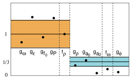
Figure 46: Comparison of the large $N$ predictions for the strengths of the various terms in the Nijmegen potential [57, 58]. The ratios of couplings (relative to $f_{\rho}$) have been plotted, and the expected size of the ratio is shown by a horizontal line. The shaded regions are an estimate of the size of the $\mathcal{O}\left(1/N\right)$ corrections to the leading result.

9 Large N and Chiral Perturbation Theory

The large $N$ expansion for baryons can be combined with baryon chiral perturbation theory [32, 59]. In the large $N$ limit, the baryon is heavy, and one can use the formalism of refs. [60]. The pion-baryon constant is order $\sqrt{N}$. The one-loop correction to the pion-baryon coupling constant is shown in fig. 47.

Figure 47: One loop correction to the pion-baryon vertex.

The diagrams produce a correction to the pion-nucleon coupling constant of the form

$$\delta g\propto Ng^{3}m_{q}\log m_{q}/\mu$$ (78)

Here $g\sqrt{N}$ is a generic pion-baryon coupling, $m$ is a light quark mass, and $\mu$ is the scale parameter of dimensional regularization. For simplicity, I will denote the light quark masses by $m_{q}$, and not distinguish between the $u$, $d$ and $s$ quark masses. One can see from eq. (78) that the chiral expansion naively breaks down in the large $N$ limit, since the correction grows with $N$. This would be true if one computed the diagrams in fig. 47 by only including intermediate nucleon states. However, in the large $N$ limit, the $\Delta$-nucleon mass difference is of order $1/N$, and the $\Delta$ must be included as an intermediate state as well. In the notation of section 1, the diagrams in fig. 47 are proportional to the group-theoretic factor

$$-2X^{ia}X^{jb}X^{ia}+X^{ia}X^{jb}X^{jb}+X^{jb}X^{jb}X^{ia}.$$ (79)

The first term in eq. (79) is the vertex correction, and the last two terms are from wavefunction renormalization. The relative factor of $-1/2$ for the wavefunction diagrams arises since their contribution to the amplitude is $1/\sqrt{Z}$. The sum over mesons is the sum on $ia$, and the sum over intermediate baryons is the matrix multiplication of $X$. Equation (79) is the double commutator

$$\left[X^{ia},\left[X^{ia},X^{ib}\right]\right]=\mathcal{O}\left(1/N^{2}\right)$$

which is of order $1/N^{2}$ from the consistency conditions of section 1. This converts eq. (78) into

$$\delta g\propto{1\over N}g^{3}m_{q}\log m_{q}/\mu,$$

and the expansion parameter is now suppressed by one power of $N$. Including the entire tower of large $N$ baryon states is crucial for this $1/N$ suppression; the double commutator is $\mathcal{O}\left(1\right)$ if only intermediate nucleon states are included. The loop expansion in the baryon sector is now a $1/N$ expansion, as in the meson sector. Hadronic dynamics in the meson and baryon sectors becomes semiclassical in the large $N$ limit [61]. The consistency conditions of section 1 can be derived by requiring that the chiral expansion has a sensible large $N$ limit [32].

It is interesting to see what happens if one studies $\pi$-nucleon scattering in the large $N$ limit without including the complete tower of large $N$ states. The nucleon is infinitely heavy in this limit, and the theory reduces to a strong coupling theory of pions interacting with a static nucleon, a model studied by Pauli and Dancoff [62]. They showed that the theory produces an infinite tower of states with $I=J=1/2,3/2,\ldots$, precisely the spectrum of the baryon tower in large $N$ QCD. The ratios of the pion-couplings are also the same as those of large $N$ QCD. One therefore has two possible ways of thinking about baryon chiral perturbation theory: (a) One starts with a Lagrangian with pions and nucleons. The theory is strongly coupled, with loop graphs of order $N$, and dynamically generates a $\Delta$ resonance. (b) One starts with a Lagrangian with pions, nucleons and $\Delta$ fields. The theory is weakly coupled, with loop graphs of order $1/N$. All predictions of (a) and (b) for observable quantities are the same. The main effect of the $\mathcal{O}\left(N\right)$ strong interactions in (a) is to produce a $\Delta$ resonance. Once the effects of this resonance are explicitly included, as in (b), the residual interactions are $\mathcal{O}\left(1/N\right)$ and weak.

Baryon chiral perturbation theory can be formulated including intermediate $\Delta$ states [60], and has been applied to baryon axial couplings, masses, magnetic moments, etc. [63, 64, 65]. Results including the $\Delta$ resonance provide a good description of the experimental data. In fact, these original calculations showed that baryon couplings were very close to their $SU(6)$ values, that there were interesting cancellations in diagrams when the $\Delta$ was included, and that ignoring the $\Delta$ led to disagreement with experiment. The large $N$ approach to baryons originated in trying to understand these results.

10 Conclusions

The $1/N$ expansion is an extremely useful tool for understanding the properties of mesons and baryons. S. Coleman, at the end of his 1979 Erice Lectures [3] remarks that “For the baryons, things are not so good. Witten’s theory is an analytical triumph but a phenomenological disaster.” He also concludes “I feel future progress in this field rests upon constructing the leading approximation.” Since these remarks much has been learned. The leading approximation (i.e. the master field) has been constructed only for $1+1$ dimensional chromodynamics, not for $3+1$ dimensional chromodynamics. Nevertheless, a lot of progress has been made. Many of the applications to mesons phenomenology in section 4 are new. Baryon phenomenology is also very successful; the new results exploit large $N$ spin-flavor symmetry, rather than the Hartree picture of Witten.

11 Acknowledgments

I would like to thank the organizers R. Gupta, A. Morel, and E. de Rafael for making this a successful Les Houches summer school. I would also like to thank R. Lebed for providing me with his ’t Hooft model computer programs, and R. Flores, Z. Ligeti, E. Poppitz and W. Skiba for carefully reading the manuscript. This work was supported in part by Department of Energy Grant DOE-FG03-97ER40546.

References

- [1] G. ’t Hooft, Nucl. Phys. B72 (1974) 461.
- [2] G. ’t Hooft, Nucl. Phys. B75 (1974) 461.
- [3] S. Coleman, , in Aspects of Symmetry, Cambridge University Press, Cambridge, 1985.
- [4] E. Witten, Nucl. Phys. B149 (1979) 285, Ann. Phys. 128 (1980) 363.
- [5] E. Witten, Nucl. Phys. B160 (1979) 57.
- [6] E. Brezin and S.R. Wadia (editors), The large expansion in quantum field theory and statistical physics: from spin systems to two-dimensional gravity, World Scientific, Singapore, 1993.
- [7] D.J. Gross and A. Neveu, Phys. Rev. D10 (1974) 3235.
- [8] G. Veneziano, Nucl. Phys. B117 (1976) 519.
- [9] D.J. Gross and W. Taylor IV, Nucl. Phys. B400 (1993) 181.
- [10] B. Grinstein and R.F. Lebed, Phys. Rev. D57 (1998) 1366.
- [11] R. Gopakumar and D.J. Gross, Nucl. Phys. B451 (1995) 379.
- [12] M.R. Douglas, Phys. Lett. B344 (1995) 117.
- [13] V.A. Kazakov and I.K. Kostov, Phys. Lett. 105B (1981) 453.
- [14] J. Greensite and M.B. Halpern, Phys. Rev. D27 (1983) 2545.
- [15] S. Coleman and E. Witten, Phys. Rev. Lett. 45 (1980) 100.
- [16] J. Gasser and H. Leutwyler, Nucl. Phys. B250 (1985) 517.
- [17] S. Peris and E. de Rafael, Phys. Lett. B348 (1995) 539.
- [18] A. Pich, Rep. Prog. Phys. 58 (1995) 563.
- [19] S. Weinberg, Physica 96A (1979) 327.
- [20] A.V. Manohar and H. Georgi, Nucl. Phys. B234 (1984) 189.
- [21] M. Fukugita, T. Inami, N. Sakai, and S. Yazaki, Phys. Lett. B72 (1977) 237.
- [22] R.S. Chivukula, J.M. Flynn and H. Georgi, Phys. Lett. B171 (1986) 453.
- [23] W.A. Bardeen, A.J. Buras and J.-M. Gerard, Phys. Lett. B180 (1986) 133, B192 (1987) 138.
- [24] B.D. Gaiser, T. Tsao and M.B. Wise, Ann. Phys. 132 (1981) 66.
- [25] G. Kilcup, R. Gupta, and S.R. Sharpe, hep-lat/9707006.
- [26] JLQCD Collaboration, S. Aoki et al., hep-lat/9710073.
- [27] G. Veneziano, Nucl. Phys. B159 (1979) 213.
- [28] H. Georgi, Phys. Rev. D49 (1994) 1666.
- [29] S. Peris, Phys. Lett. B324 (1994) 442.
- [30] P. Herrera-Siklody, J.I. Lattore, P. Pascual, and J. Taron, Nucl. Phys. B497 (1997) 345.
- [31] G. Karl and J.E. Paton, Phys. Rev. D30 (1984) 238.
- [32] R. Dashen and A.V. Manohar, Phys. Lett. B315 (1993) 425, 438.
- [33] J.-L. Gervais and B. Sakita, Phys. Rev. Lett. 52 (1984) 87; Phys. Rev. D30 (1984) 1795.
- [34] A.V. Manohar, Nucl. Phys. B248 (1984) 19.
- [35] R. Dashen, E. Jenkins and A.V. Manohar, Phys. Rev. D49 (1994) 4713.
- [36] R. Dashen, E. Jenkins and A.V. Manohar, Phys. Rev. D51 (1995) 3697.
- [37] E. Jenkins, Phys. Lett. B315 (1993) 431, 441, 447.
- [38] G.S. Adkins, C.R. Nappi, and E. Witten, Nucl. Phys. B228 (1983) 552.
- [39] C. Carone, H. Georgi, and S. Osofsky, Phys. Lett. B322 (1994) 227.
- [40] M. Luty and J. March-Russell, Nucl. Phys. B426 (1994) 71; M. Luty, Phys. Rev. D51 (1995) 2322.
- [41] E. Jenkins and R.F. Lebed, Phys. Rev. D52 (1995) 282.
- [42] E. Jenkins and A.V. Manohar, Phys. Lett. B335 (1994) 452.
- [43] M. Luty, J. March-Russell, and M. White, Phys. Rev. D51 (1995) 2332.
- [44] J. Dai, R. Dashen, E. Jenkins, and A.V. Manohar, Phys. Rev. D53 (1996) 273.
- [45] D.B. Kaplan and M.J. Savage, Phys. Lett. B365 (1996) 244.
- [46] D.B. Kaplan and A.V. Manohar, Phys. Rev. C56 (1997) 76.
- [47] C. Carone, H. Georgi, L. Kaplan and D. Morin, Phys. Rev. D50 (1994) 5793.
- [48] G.L Goity, Phys. Lett. B414 (1997) 140.
- [49] D. Pirjol and T.-M. Yan, hep-ph/9707485, hep-ph/9711201.
- [50] E. Jenkins, Phys. Rev. D54 (1996) 4515.
- [51] E. Jenkins, A.V. Manohar, and M.B. Wise, Nucl. Phys. B396 (1993) 27-37; Z. Guralnik, M.E. Luke, and A.V. Manohar, Nucl. Phys. B390 (1993) 474.
- [52] C.-K. Chow, Phys. Rev. D54 (1996) 873.
- [53] G.S. Adkins and C.R. Nappi, Nucl. Phys. B249 (1985) 507.
- [54] M.P. Mattis and M. Mukherjee, Phys. Rev. Lett. 61 (1988) 1344.
- [55] M.P. Mattis, Phys. Rev. D39 (1989) 994.
- [56] M.P. Mattis and E. Braaten, Phys. Rev. D39 (1989) 2737.
- [57] M.M. Nagels, T.A. Rijken, and J.J. de Swart, Phys. Rev. D17 (1978) 768.
- [58] V.G.J. Stoks, R.A.M. Klomp, C.P.F. Terheggen, and J.J. de Swart, Phys. Rev. C49 (1994) 2950.
- [59] E. Jenkins, Phys. Rev. D53 (1996) 2625.
- [60] E. Jenkins and A.V. Manohar, Phys. Lett. B255 (1991) 558, B259 (1991) 353.
- [61] A.V. Manohar, Phys. Lett. B336 (1994) 502.
- [62] W. Pauli and S. Dancoff, Phys. Rev. 62 (1942) 85.
- [63] E. Jenkins and A.V. Manohar, in Effective Field Theories of the Standard Model, edited by U. Meissner, World Scientific, Singapore, 1992.
- [64] E. Jenkins, M.E. Luke, A.V. Manohar, and M.J. Savage, Phys. Lett. B302 (1993) 482, Nucl. Phys. B397 (1993) 84.
- [65] E. Jenkins, Nucl. Phys. B368 (1992) 190, Nucl. Phys. B375 (1992) 561.