Mixing and Decay Constants of Pseudoscalar Mesons

Abstract

We propose a new $\eta$–$\eta^{\prime}$ mixing scheme where we start from the quark flavor basis and assume that the decay constants in that basis follow the pattern of particle state mixing. On exploiting the divergences of the axial vector currents – which embody the axial vector anomaly – all basic parameters are fixed to first order of flavor symmetry breaking. That approach naturally leads to a mass matrix, quadratic in the masses, with specified elements. We also test our mixing scheme against experiment and determine corrections to the first order values of the basic parameters from phenomenology. Finally, we generalize the mixing scheme to include the $\eta_{c}$. Again the divergences of the axial vector currents fix the mass matrix and, hence, mixing angles and the charm content of the $\eta$ and $\eta^{\prime}$.

I Introduction

$\eta$–$\eta^{\prime}$ mixing is a subject of considerable interest that has been examined in many investigations, see e.g. [1, 2, 3, 4] and references therein. As it is well-known [5], the ${\rm U}(1)_{\rm A}$ anomaly plays a decisive role. For the octet-singlet mixing angle $\theta$ of these pseudoscalar mesons values in the range of $-10^{\circ}$ to $-23^{\circ}$ have been obtained depending on details of the analysis, see e.g. [3]. The phenomenological analysis often involves decay processes where, besides state mixing, also weak decay constants appear. The decay constants are defined by

$$\langle 0|J_{\mu 5}^{i}|P(p)\rangle=\imath\,f_{P}^{i}\,p_{\mu}\qquad(i=8,1;\quad P=\eta,\eta^{\prime})\,,$$ (1)

where $J_{\mu 5}^{8}$ denotes the ${\rm SU}(3)_{{\rm F}}$ octet and $J_{\mu 5}^{1}$ the ${\rm SU}(3)_{{\rm F}}$ singlet axial-vector current, respectively. Frequently, it is assumed that the decay constants follow the pattern of state mixing:

$$f_{\eta\phantom{{}^{\prime}}}^{8}=f_{8}\,\cos\theta\ ,\qquad f_{\eta\phantom{{}^{\prime}}}^{1}=-f_{1}\,\sin\theta\ ,$$ (2)

$$f_{\eta^{\prime}}^{8}=f_{8}\,\sin\theta\ ,\qquad f_{\eta^{\prime}}^{1}=\phantom{-}f_{1}\,\cos\theta\ .$$ (3)

However, recent theoretical [6] as well as phenomenological [7] investigations have shown that Eq. (3) cannot be correct. Adopting the new and general parametrization [6]

$$f_{\eta\phantom{{}^{\prime}}}^{8}=f_{8}\,\cos\theta_{8}\ ,\qquad f_{\eta\phantom{{}^{\prime}}}^{1}=-f_{1}\,\sin\theta_{1}\ ,$$ (4)

$$f_{\eta^{\prime}}^{8}=f_{8}\,\sin\theta_{8}\ ,\qquad f_{\eta^{\prime}}^{1}=\phantom{-}f_{1}\,\cos\theta_{1}\ .$$ (5)

$\theta_{1}$ and $\theta_{8}$ turned out to differ considerably. The phenomenological analysis [7], which involved the combined analysis of the two-photon decay widths of the $\eta$ and $\eta^{\prime}$, the $\eta\gamma$ and $\eta^{\prime}\gamma$ transition form factors and the additional constraint from the radiative $J/\psi$ decays, allowed to determine the four quantities occuring in Eq. (5). Most importantly, the values obtained satisfy the constraints [6] from chiral perturbation theory (ChPT).

The appearance of the four parameters $f_{8},f_{1},\theta_{8},\theta_{1}$ raises anew the problem of their mutual relations and their connection with the mixing angle of the particle states. This angle is necessarily a single one since mixing with higher states – the $\eta_{{\rm{c}}}$ for instance – can be neglected at this stage. The relation of this angle with the four parameters in Eq. (5) does not need to be simple: in a parton language [8] the decay constants are controlled by specific Fock state wave functions at zero spatial separation of the quarks while state mixing refers to the mixing in the overall wave functions.

In this work we express $\eta$ and $\eta^{\prime}$ as linear combinations of orthogonal states $\eta_{\rm{q}}$ and $\eta_{{\rm{s}}}$ which can be generated by the axial vector currents with the flavor structure ${\rm q}\overline{\rm q}=({\rm u}\overline{\rm u}+{\rm d}\overline{\rm d})/\sqrt{2}$ and ${\rm s}\overline{\rm s}$, respectively. They are chosen in such a way that both states have vanishing vacuum-particle matrix elements with the opposite currents, i.e. their lowest Fock space components have the compositions ${\rm q}\overline{\rm q}$ and ${\rm s}\overline{\rm s}$, respectively. Our motivation for choosing this specific basis comes from the fact that the breaking of ${\rm SU}(3)_{{\rm F}}$ by the quark masses influences the two parts differently, and from the observation that vector and tensor mesons – where the axial vector anomaly plays no role – have state mixing angles very close to the ideal mixing angle $\theta_{ideal}=\arctan\sqrt{2}$. We will demonstrate that the proper use of this quark flavor basis provides for new insights and successful predictions. We point out that we employ fixed (momentum-independent) basis states. Thus, our state mixing angle is momentum independent and well-defined also in any other basis obtained by an orthogonal transformation. This differs from other possible approaches in which momentum dependent mass matrices are introduced (see, for instance, [9]). The decay constants, on the other hand, will in general depend on $q^{2}$, i.e. the particle states and masses, and will thus require a parametrization by two different mixing angles as in (5). These angles depend on the basis which is used for the definition of the decay constants. As described below, the basic assumption which we will use in this paper is that the decay constants follow the state mixing if and only if they are defined with respect to the quark basis. In this circumstance the two angles for the decay constants obtained in this basis and the corresponding state mixing angle coincide and are thus momentum-independent.

Defining now decay constants analogous to Eq. (1) but with $i=\rm{q},{\rm{s}}$ and denoting the $\eta$ – $\eta^{\prime}$ mixing angle that describes the deviation from ideal mixing, by $\phi$, we propose

$$f_{\eta}^{\rm{q}}=f_{\rm{q}}\,\cos\phi\ ,\qquad f_{\eta}^{{\rm{s}}}=-f_{{\rm{s}}}\,\sin\phi\ ,\nopagebreak$$ (6)

$$f_{\eta^{\prime}}^{\rm{q}}=f_{\rm{q}}\,\sin\phi\ ,\qquad f_{\eta^{\prime}}^{{\rm{s}}}=\ \ f_{{\rm{s}}}\,\cos\phi\ .$$ (7)

That the decay constants in the quark flavor basis follow in this way the pattern of particle state mixing is our central assumption. It is equivalent to the requirement that the contribution $f_{\rm{q}}$ ($f_{{\rm{s}}}$) to the decay constants obtained from the $\eta_{\rm{q}}$ ($\eta_{{\rm{s}}}$) components of the wave functions is independent of the meson involved. This assumption appears plausible but we have no rigorous justification for it and have to test it. It is certainly restrictive as will be shown in Sect. II: first, it reduces the number of parameters again to three. Secondly, by invoking the divergences of the currents, the angle $\phi$ is connected to $f_{\rm{q}}/f_{{\rm{s}}}$. Finally, flavor symmetry fixes $f_{\rm{q}}$ and $f_{{\rm{s}}}$ to first order of ${\rm SU}(3)_{{\rm F}}$ breaking, leaving us – to this order – with no free parameter. Mass mixing of the pseudoscalar mesons is also discussed in this section. Numerous phenomenological checks are possible and performed in Sect. III. We determine phenomenological values for the three parameters from the data and check for consistency with ChPT and the earlier determination [7] of the four quantities $f_{8},f_{1},\theta_{8},\theta_{1}$. Our scheme will then be generalized to include the $\eta_{{\rm{c}}}$ in Sect. IV. The generalized approach allows to estimate the quark content of the three pseudoscalar mesons, the mixing angles and the charm decay constants $f^{{\rm{c}}}_{\eta}$ and $f^{{\rm{c}}}_{\eta^{\prime}}$ which attracted much interest in the current discussion [10, 11, 12, 13] of the rather large branching ratio for the process $B\to K\eta^{\prime}$ as measured by CLEO [14]. Our summary is presented in Sect. V.

II The ${\rm q}\overline{\rm q}$ – ${\rm s}\overline{\rm s}$ mixing scheme

The two states $\eta_{\rm{q}}$ and $\eta_{{\rm{s}}}$ are related to the physical states by the transformation

$$\left(\matrix{\eta\cr\eta^{\prime}}\right)\,=\,U(\phi)\;\left(\matrix{\eta_{\rm{q}}\cr\eta_{{\rm{s}}}}\right),$$ (8)

where $U$ is a unitary matrix defined by

$$U(\alpha)\,=\,\left(\matrix{\cos{\alpha}&-\sin{\alpha}\cr\sin{\alpha}&\phantom{-}\cos{\alpha}}\right).$$ (9)

We assume that the physical states are orthogonal, i.e. that mixing with heavier pseudoscalar mesons (e.g. the $\eta_{{\rm{c}}}$) can be ignored, see, however, Sect. IV. We stress that as long as state-mixing is considered, one may freely transform from one orthogonal basis to the other. For example, the standard octet-singlet mixing angle is given by $\theta=\phi-\theta_{\rm ideal}$. According to our central assumption described in Sect. 1, we take

$$\left(\matrix{f_{\eta}^{\rm{q}}&f_{\eta}^{{\rm{s}}}\cr f_{\eta^{\prime}}^{\rm{q}}&f_{\eta^{\prime}}^{{\rm{s}}}}\right)\,=\,U(\phi)\;{\mathcal{F}}\ ,\quad{\mathcal{F}}\,=\,\left(\matrix{f_{\rm{q}}&0\cr 0&f_{{\rm{s}}}}\right).$$ (10)

Transforming the non-strange and strange axial-vector currents into octet and singlet currents, one can also connect the decay constants defined in Eq. (1) to $f_{\rm{q}}$ and $f_{{\rm{s}}}$

$$\left(\matrix{f_{\eta}^{8}&f_{\eta}^{1}\cr f_{\eta^{\prime}}^{8}&f_{\eta^{\prime}}^{1}}\right)\,=\,U(\phi)\;{\mathcal{F}}\;U^{\dagger}(\theta_{ideal})$$ (11)

with the result

$$f_{8}=\sqrt{1/3\,f_{\rm{q}}^{2}+2/3\,f_{{\rm{s}}}^{2}}\ ,\qquad\theta_{8}=\phi-\arctan(\sqrt{2}\,f_{{\rm{s}}}/f_{\rm{q}})\ ,$$ (12)

$$f_{1}=\sqrt{2/3\,f_{\rm{q}}^{2}+1/3\,f_{{\rm{s}}}^{2}}\ ,\qquad\theta_{1}=\phi-\arctan(\sqrt{2}\,f_{\rm{q}}/f_{{\rm{s}}})\$$ (13)

and thus

$$\tan(\theta_{1}-\theta_{8})=\sqrt{2}/3\,(f_{{\rm{s}}}/f_{\rm{q}}-f_{\rm{q}}/f_{{\rm{s}}})~{}.$$ (14)

These results clearly show that, as a consequence of ${\rm SU}(3)_{{\rm F}}$ breaking, at most for a single choice of the basis states the matrix of the decay constants follows the particle state mixing as in Eq. (10). For the reasons mentioned in the introduction we assume Eq. (10) to hold in the ${\rm q}\overline{\rm q}$-${\rm s}\overline{\rm s}$ basis. It implies that the decay constants of the mesons are mass independent superpositions of $f_{\rm{q}}$ and $f_{{\rm{s}}}$. The difference between our ansatz for the decay constants and the customary ones lies in the treatment of ${\rm SU}(3)_{{\rm F}}$ breaking effects, which naturally manifest themselves in the ratio $f_{\rm{q}}/f_{{\rm{s}}}\neq 1$. In order to proceed we consider the divergences of the axial vector currents. They embody the well-known axial vector anomaly, for instance

$$\partial^{\mu}J_{\mu 5}^{{\rm{s}}}=\partial^{\mu}(\bar{{\rm{s}}}\,\gamma_{\mu}\gamma_{5}\,{\rm{s}}) = 2\,m_{{\rm{s}}}\,(\bar{{\rm{s}}}\,i\gamma_{5}\,{{\rm{s}}})+\frac{\alpha_{s}}{4\pi}\,G\,\tilde{G}\ .$$ (15)

$G$ denotes the gluon field strength tensor and $\tilde{G}$ its dual; $m_{i}$ denote the current quark masses. The vacuum–meson transition matrix elements of the axial vector current divergences are given by the product of the square of the meson mass, $M_{P}^{2}$, and the appropriate decay constant. For instance,

$$\langle 0|\partial^{\mu}J_{\mu 5}^{{\rm{s}}}|\eta\rangle=M_{\eta}^{2}\,f_{\eta}^{{\rm{s}}}\ .$$ (16)

The mass factors, which necessarily appear quadratically here, can be considered as the elements of the particle mass matrix

$${\mathcal{M}}^{2}=\left(\matrix{M_{\eta}^{2}&0\cr 0&M_{\eta^{\prime}}^{2}}\right)\ .$$ (17)

With the help of Eq. (10) the matrix elements of $\partial^{\mu}J_{\mu 5}^{i}$ ($i=q,s$) can then be identified as those of the matrix product ${\mathcal{M}}^{2}\,U(\phi)\,{\mathcal{F}}$. Transforming it to the quark flavor basis and solving for the mass matrix

$${\mathcal{M}}^{2}_{\rm{q}{\rm{s}}}=U^{\dagger}(\phi)\,{\mathcal{M}}^{2}\,U(\phi)\ ,$$ (18)

one easily finds

$${\mathcal{M}}^{2}_{\rm{q}{\rm{s}}}=\left(\matrix{m_{\rm{q}\rm{q}}^{2}+\frac{\sqrt{2}}{f_{\rm{q}}}\,\langle 0|\frac{\alpha_{s}}{4\pi}\,G\tilde{G}|\eta_{\rm{q}}\rangle&\frac{1}{f_{{\rm{s}}}}\,\langle 0|\frac{\alpha_{s}}{4\pi}\,G\tilde{G}|\eta_{\rm{q}}\rangle\vspace{0.3em}\cr\frac{\sqrt{2}}{f_{\rm{q}}}\,\langle 0|\frac{\alpha_{s}}{4\pi}\,G\tilde{G}|\eta_{{\rm{s}}}\rangle&m_{{\rm{s}}{\rm{s}}}^{2}+\frac{1}{f_{{\rm{s}}}}\,\langle 0|\frac{\alpha_{s}}{4\pi}\,G\tilde{G}|\eta_{{\rm{s}}}\rangle}\right)$$ (19)

where we use the abbreviations

$$m_{\rm{q}\rm{q}}^{2}=\frac{\sqrt{2}}{f_{\rm{q}}}\,\langle 0|m_{\rm{u}}\,\bar{\rm{u}}\,i\gamma_{5}\,{\rm{u}}+m_{\rm{d}}\,\bar{\rm{d}}\,i\gamma_{5}\,{\rm{d}}|\eta_{\rm{q}}\rangle;\quad m_{{\rm{s}}{\rm{s}}}^{2}=\frac{2}{f_{{\rm{s}}}}\,\langle 0|m_{{\rm{s}}}\,\bar{{\rm{s}}}\,i\gamma_{5}\,{{\rm{s}}}|\eta_{{\rm{s}}}\rangle$$ (20)

for the quark mass contributions to ${\mathcal{M}}_{\rm{q}{\rm{s}}}^{2}$. As expected, the anomaly is the only source of the non-diagonal elements. The symmetry of the mass matrix forces an important connection between the ratio of couplings of our basis states to the anomaly

$$y=\sqrt{2}\,\frac{\langle 0|\frac{\alpha_{s}}{4\pi}\,G\tilde{G}|\eta_{{\rm{s}}}\rangle}{\langle 0|\frac{\alpha_{s}}{4\pi}\,G\tilde{G}|\eta_{\rm{q}}\rangle}=\frac{f_{\rm{q}}}{f_{{\rm{s}}}}\ .$$ (21)

For later use it is also convenient to introduce the abbreviation

$$a^{2}=\frac{1}{\sqrt{2}\,f_{\rm{q}}}\,\langle 0|\frac{\alpha_{s}}{4\pi}\,G\tilde{G}|\eta_{\rm{q}}\rangle$$ (22)

for the anomaly contribution to the mass matrix. On account of Eqs. (18) and (19) both, $a^{2}$ and $y$, can be expressed in terms of the masses and the mixing angle $\phi$

$$a^{2} = \frac{M_{\eta}^{2}\,\cos^{2}\phi+M_{\eta^{\prime}}^{2}\,\sin^{2}\phi-m_{\rm{q}\rm{q}}^{2}}{2}\,,$$ (23)

$$y = \frac{(M_{\eta^{\prime}}^{2}-M_{\eta}^{2})\,\sin 2\phi}{2\sqrt{2}\,a^{2}}\,.$$ (24)

The combination of Eqs. (21) and (24) provides an interesting relation between $f_{\rm{q}}/f_{{\rm{s}}}$ and the mixing angle $\phi$. Also worth noting is the relation between $\phi$ and $\theta_{8}$ that is obtained by combining Eq. (13) with Eqs. (21) and (24)

$$\cot\theta_{8}\,=\,-\,\frac{M_{\eta^{\prime}}^{2}}{M_{\eta}^{2}}\,\tan\phi.$$ (25)

This relation holds up to corrections of order $m_{\rm{q}\rm{q}}^{2}/M^{2}_{P}$.

Flavor symmetry allows to relate $m_{\rm{q}\rm{q}}^{2}$ and $m_{{\rm{s}}{\rm{s}}}^{2}$, defined in Eq. (20), to the pion and kaon masses. To the order we are working, one gets

$$m_{\rm{q}\rm{q}}^{2}=M_{\pi}^{2}\ ,\quad m_{{\rm{s}}{\rm{s}}}^{2}=2\,M_{K}^{2}-M_{\pi}^{2}\ .$$ (26)

These relations allow for a first and – to the given order – parameter-free application of our scheme for the determination of all quantities relevant for $\eta$–$\eta^{\prime}$ mixing provided the values of the physical particle masses are given. Using Eqs. (23) and (24) as well as Eq. (26) for the corresponding elements of the mass matrix (19), we evaluate $\phi$, $a^{2}$ and $y$, and hence $\theta$. The results for these quantities are listed in Table I.

For a theoretical estimate of $f_{\rm{q}}$ and $f_{{\rm{s}}}$ we take over their particle independence which was necessary for Eq. (7) to hold, to the $\pi$ and the $K$ meson. We retain the difference between the pion and kaon decay constants as a first order correction due to flavor symmetry breaking:

$$f_{\rm{q}}=f_{\pi}\ ,\qquad f_{{\rm{s}}}=\sqrt{2\,f_{K}^{2}-f_{\pi}^{2}}~{}.$$ (27)

Note that $V$-spin considerations provide a linear relation between the decay constants $f_{{\rm{s}}}$, $f_{\pi}$ and $f_{K}$ which, to the considered order of flavor symmetry breaking, can be replaced by the above quadratic relation. As can be seen from Eq. (14), these theoretical results for $f_{\rm{q}}$ and $f_{{\rm{s}}}$ lead to a substantial difference between $\theta_{1}$ and $\theta_{8}$. Only in the strict ${\rm SU}(3)_{{\rm F}}$ limit where $f_{\rm{q}}=f_{{\rm{s}}}$ (or, equivalently, $f_{K}=f_{\pi}$ or $f_{8}=f_{1}$) one would have $\theta_{1}=\theta_{8}=\theta$, with $\theta$ being the octet-singlet mixing angle. According to Leutwyler [6], ChPT provides two relations (up to $1/N_{c}$ corrections) among the decay constants

$$f_{8}=\sqrt{\frac{4}{3}\,f_{K}^{2}-\frac{1}{3}\,f_{\pi}^{2}}\ ,\qquad f_{\eta}^{8}\,f_{\eta}^{1}+f_{\eta^{\prime}}^{8}\,f_{\eta^{\prime}}^{1}=-\frac{2\sqrt{2}}{3}\,(f_{K}^{2}-f_{\pi}^{2}).$$ (28)

It can easily be verified that, on using Eq. (27), these relations are satisfied in our approach. By means of Eq. (13) the theoretical values of $f_{8}$, $f_{1}$, $\theta_{8}$ and $\theta_{1}$ are determined by the decay constants presented in Eq. (27) and the mixing angle $\phi$ computed from the mass matrix (see Table II below). The numerical values of the mixing parameters, resulting from Eqs. (26),(27), may, of course, be subject to sizeable corrections (of $O(1/N_{c})$ in the language of ChPT). As an example of the size of such corrections we note that from Eqs. (27) and (21) $y=0.71$ follows which differs from the value obtained from the mass matrix, see Table I. The corrections to the mixing parameters will phenomenologically be estimated in the next section.

The considerations presented in this section nicely demonstrate that our approach is indeed very restrictive. To the order of flavor symmetry breaking we are working, there is no free parameter left. As is to be emphasized this interesting outcome crucially depends on the central assumption (7). If, in analogy to Eq. (5), we allowed for two angles in the quark flavor basis for the parametrization of the decay constants, our approach would loose its predictive power completely. In the next section we will confront our approach with experiment. We determine the mixing angle $\phi$ and the basic decay constants $f_{\rm{q}}$ and $f_{{\rm{s}}}$ phenomenologically and look for consistency and for deviations from the first order of ${\rm SU}(3)_{{\rm F}}$ breaking.

III The phenomenological values of $\phi$, $f_{\rm{q}}$, $f_{{\rm{s}}}$

Several possibilities to extract the value of the mixing angle from experiment have been discussed in the literature, see, for instance, [1, 3, 15, 16]. We can profit from these papers by properly adapting them to the $\rm{q}\overline{\rm{q}}-{\rm{s}}\overline{\rm{s}}$ mixing scheme. We note that in the phenomenological analyses [1, 3, 15, 16] some additional simplifying assumptions had to be made. Thus, for instance, OZI-suppressed contributions or mass dependencies of form factors and coupling constants are ignored. We start by first discussing processes which are independent (or insensitive) to the decay constants and allow a one parameter fit of the particle state mixing angle $\phi$.

• The decay $J/\psi\to P\rho$: We consider the ratio of the decay widths $\Gamma[J/\psi\to\eta^{\prime}\rho]$ and $\Gamma[J/\psi\to\eta\phantom{{}^{\prime}}\rho]$. In these processes $G$-parity is not conserved, they proceed through a virtual photon (see Fig. 1a). Contributions from the isospin-violating part of QCD are supposedly very small as can be inferred from the smallness of the $J/\psi\to\phi\pi$ width and will be neglected. The calculation of the decay widths requires the knowledge of the $\rho$–$P$ transition form factors at momentum transfer $q^{2}=M_{J/\psi}^{2}$. On account of the flavor content of the $\rho$ meson, this transition form factor only probes the $\eta_{\rm{q}}$ components of the $\eta$ and $\eta^{\prime}$ if OZI-suppressed contributions are neglected. Hence,

  $$F_{\rho\eta\phantom{{}^{\prime}}}(q^{2}) = \cos\phi\,F_{\rho\eta_{\rm{q}}}(q^{2}),$$ (29)

  $$F_{\rho\eta^{\prime}}(q^{2}) = \sin\phi\,F_{\rho\eta_{\rm{q}}}(q^{2})\,.$$ (30)

  and therefore

  $$\frac{\Gamma[J/\psi\to\eta^{\prime}\rho]}{\Gamma[J/\psi\to\eta\phantom{{}^{\prime}}\rho]}=\tan^{2}\phi\,\left(\frac{k_{\eta^{\prime}\rho}}{k_{\eta\phantom{{}}\rho}}\right)^{3}$$ (31)

  where

  $$k_{PV}=M_{J/\psi}\,[1-(M_{P}^{2}+M_{V}^{2})/M_{J/\psi}^{2}]\,/2.$$ (32)

  From the experimental value $0.54\pm 0.11$ for this ratio of decay widths [17] we obtain $\phi=39.9^{\circ}\pm 2.9^{\circ}$. Almost the same value for $\phi$ has been found in an analysis of all isospin-1 $J/\psi\to PV$ decays (including pions)[16]. A global fit to all $J/\psi\to PV$ decay modes on the basis of a particular model, yields $\phi=37.8^{\circ}\pm 1.7^{\circ}$[16]. Because of its model dependence we will not use the latter result in evaluating the average of the mixing angle. Since in the derivation of Eq. (31) only the mixing angle of the particle states enters, one may freely transform from the $\rm{q}\overline{\rm{q}}-s\overline{\rm{s}}$ basis to the octet-singlet one as was done, for instance, in [16]. Nevertheless, the simple relation between the ratio of decay widths and the mixing angle, independent of the dynamics, is an advantage of the $\rm{q}\overline{\rm{q}}-{\rm{s}}\overline{\rm{s}}$ basis used here. In the octet-singlet mixing scheme one would have to deal with a linear combination of two a priori different form factors. We will profit from this advantage also in the following five processes.

• The decays $\eta^{\prime}\to\rho\gamma$ and $\rho\to\eta\gamma$: The transition matrix elements controlling these processes can be decomposed covariantly [18]

  $$\langle\gamma P(p_{P})|T|\rho(p_{\rho})\rangle=-eg_{\rho P\gamma}\,\epsilon_{\mu\nu\lambda\sigma}\,p_{P}^{\mu}\,\varepsilon_{\gamma}^{(*)\nu}\,p_{\rho}^{\lambda}\varepsilon_{\rho}^{\sigma}\,,$$ (33)

  leading to the following expressions for the decay widths

  $$\Gamma[\eta^{\prime}\to\rho\gamma]=\alpha\,g_{\rho\eta^{\prime}\gamma}^{2}\,k_{\rho}^{3}\ ,\qquad\Gamma[\rho\to\eta\gamma]=\frac{\alpha}{3}\,g_{\rho\eta\gamma}^{2}\,k_{\eta}^{3}~{}.$$ (34)

  where

  $$k_{\rm f}=M_{\rm i}\,[1-M_{\rm f}^{2}/M_{\rm i}^{2}]/2\ ,$$ (35)

  being the 3-momenta of the final state meson f. $M_{\rm i}$ denotes the mass of the decaying meson. $\alpha$ is the fine structure constant. Using state mixing (8), one finds

  $$\frac{g_{\rho\eta^{\prime}\gamma}}{g_{\rho\eta\gamma}}\,=\,\tan{\phi}\,.$$ (36)

  From the measured decay widths [17] we obtain for the ratio of the $\rho\eta(\eta^{\prime})\gamma$ coupling constants the value $1.41\pm 0.29$ from which $\phi=35.3^{\circ}\pm 5.5^{\circ}$ follows.

• The decays $T\to P_{1}P_{2}$: Here $T$ denotes a $2^{++}$ tensor meson and $P_{i}$ refers to a pseudoscalar meson. Most suitable for a rather model-independent determination of $\phi$ are the $\eta(\eta^{\prime})\pi$ decay modes of the $a_{2}$. Using the same assumptions as before one gets

  $$\frac{\Gamma[a_{2}\to\eta^{\prime}\pi]}{\Gamma[a_{2}\to\eta\phantom{{}^{\prime}}\pi]} = \tan^{2}\phi\,\left(\frac{k_{\eta^{\prime}\pi}}{k_{\eta\phantom{{}^{\prime}}\pi}}\right)^{5}\,,$$ (37)

  where $k_{P\pi}$ is defined analogously to Eq. (32). From the experimental value for that ratio, $0.039\pm 0.008$ [17], we obtain $\phi=43.1^{\circ}\pm 3.0^{\circ}$. In [16] the whole class of $T\to P_{1}P_{2}$ decays has been analyzed in a model-dependent way recently. An overall fit to the data is consistent with $\phi\simeq 39^{\circ}$.

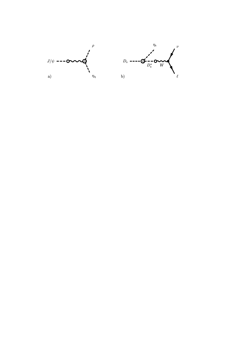
• The decay $D_{{\rm{s}}}\to Pe\nu$: The ratio of decay widths $\Gamma[D_{{\rm{s}}}\to\eta^{\prime}e\nu]/\Gamma[D_{{\rm{s}}}\to\eta e\nu]$ is determined by the $D_{{\rm{s}}}\to\eta^{\prime}$, $\eta$ form factors $f_{+}^{\eta^{\prime}}(q^{2})$ and $f_{+}^{\eta}(q^{2})$. Using a pole ansatz for their $q^{2}$ dependence [19] one can extract from the decay rates the form factor ratio at $q^{2}$= 0 which – in our scheme – is simply equal to $\cot\phi$. The analysis [15] using a monopole behavior with the $D_{{\rm{s}}}^{*}$ pole see Fig. 1b and CLEO data [20] gives the value of $1.14\pm 0.17\pm 0.13$ and, hence, $\phi=41.3^{\circ}\pm 5.3^{\circ}$.

• The scattering processes $\pi^{-}p\to Pn$: At high energies the ratio of the cross-sections should be independent of phase-space corrections and is given by [3, 16]

  $$\frac{\sigma(\pi^{-}p\to\eta^{\prime}n)}{\sigma(\pi^{-}p\to\eta\phantom{{}^{\prime}}n)} = \tan^{2}\phi\quad(s\gg M_{P}^{2})$$ (38)

  The two experiments lead to $\phi=36.5^{\circ}\pm 1.4^{\circ}$ [21] and $39.3^{\circ}\pm 1.2^{\circ}$ [22]. Since the two results are not fully consistent with each other we will double the errors in the evaluation of the averaged value $\bar{\phi}$.

• Annihilation processes $p\bar{p}\to PM$ ($M=\pi^{0},\eta,\omega$): The Crystal Barrel Collaboration [23] measured the ratios for annihilation into $\eta M$ and $\eta^{\prime}M$ and quoted a value of $\phi=37.4^{\circ}\pm 1.8^{\circ}$ for the mixing angle. However, since the experiment was carried through at low energies, the result for $\phi$ is rather sensitive to phase space factors and to the momentum dependence of the annihilation amplitudes. We therefore discard that value of $\phi$ in the determination of the averaged mixing angle although it will turn out to be consistent with it.

• The decay $J/\psi\to P\gamma$: According to [24, 15] the photon is emitted by the ${\rm{c}}$ quarks which then annihilate into lighter quark pairs through the effect of the anomaly. Thus, the creation of the corresponding light mesons is controlled by the matrix element $\langle 0|\frac{\alpha_{s}}{4\pi}G\tilde{G}|P\rangle$. The photon emission from light quarks is negligibly small as seen from the smallness of the $\pi\gamma$ decay branching ratio. Using Eqs. (19, 21) and (25) as well as setting $m_{u,d}=0$, we have

  $$R_{J/\psi}=\frac{\Gamma[J/\psi\to\eta^{\prime}\gamma]}{\Gamma[J/\psi\to\eta\phantom{{}^{\prime}}\gamma]} = \tan^{2}\phi\,\frac{M_{\eta^{\prime}}^{4}}{M_{\eta\phantom{{}^{\prime}}}^{4}}\,\left(\frac{k_{\eta^{\prime}}}{k_{\eta\phantom{{}^{\prime}}}}\right)^{3}=\cot^{2}\theta_{8}\,\left(\frac{k_{\eta^{\prime}}}{k_{\eta\phantom{{}^{\prime}}}}\right)^{3}\ .$$ (39)

  From the measured value [17] $R_{J/\psi}=5.0\pm 0.6$ the mixing angle $\phi$ becomes $39.0^{\circ}\pm 1.6^{\circ}$. Obviously, Eq. (39) is not equivalent to the naive singlet dominance prediction for which the factor $\cot\theta_{8}$ would have to be replaced by $\cot\theta$. As we learned in Sect. II, $\theta_{8}$ markedly differs from the octet-singlet mixing angle.

FIG. 1.: a) Electromagnetic contribution to $J/\psi\to\rho\eta,\eta^{\prime}$. b) Pole ansatz for the $D_{{\rm{s}}}\to P\ell\nu$ semi-leptonic decay.

A weighted average of the above seven high-lighted values yields

$$\overline{\phi}=39.3^{\circ}\pm 1.0^{\circ}.$$ (40)

Quite remarkably, the values for $\phi$ obtained from very different physical processes are all compatible with each other within the errors. This is not the case in the octet-singlet scheme ($\theta_{8}=\theta_{1}=\theta$) where values varying from $-10^{\circ}$ to $-23^{\circ}$ have been found for $\theta$ [3, 15, 16]. The phenomenological value of $\phi$ does not differ substantially from the leading order value, i.e. the higher order flavor symmetry breaking corrections, absorbed in the phenomenological value, are apparently not large (see Table I).

Having fixed the mixing angle, we are in the position to determine phenomenologically the ratio of the decay constants $f_{\rm{q}}$ and $f_{{\rm{s}}}$ by combining Eqs. (21) and (24). We find, with $m_{qq}^{2}=M_{\pi}^{2}$,

$$f_{\rm{q}}/f_{{\rm{s}}}=y=0.81\pm 0.03.$$ (41)

It is amusing to note that the replacement of the kaon mass by an effective mass of $508$ MeV in the mass matrix introduced in Sect. II reproduces the phenomenological values of $\phi$, $a^{2}$ and $y$ exactly.

• The decay $P\to\gamma\gamma$: The two-photon decays of the $\eta$ and the $\eta^{\prime}$ provide independent information on the two decay constants. Expressing the PCAC results, see [7] and references therein, for the two-photon decay widths of the $\eta$ and $\eta^{\prime}$ in terms of $\phi$, $f_{\rm{q}}$ and $f_{{\rm{s}}}$ ($C_{\rm{q}}=5/9\sqrt{2}$, $C_{{\rm{s}}}=1/9$)

  $$\Gamma[\eta\phantom{{}^{\prime}}\to\gamma\gamma] = \frac{9\alpha^{2}}{16\pi^{3}}\,M_{\eta\phantom{{}^{\prime}}}^{3}\,\left[\frac{C_{\rm{q}}\,\cos\phi}{f_{\rm{q}}}-\frac{C_{{\rm{s}}}\,\sin\phi}{f_{{\rm{s}}}}\right]^{2}\ ,$$ (42)

  $$\Gamma[{\eta^{\prime}}\to\gamma\gamma] = \frac{9\alpha^{2}}{16\pi^{3}}\,M_{{\eta^{\prime}}}^{3}\,\left[\frac{C_{\rm{q}}\,\sin\phi}{f_{\rm{q}}}+\frac{C_{{\rm{s}}}\,\cos\phi}{f_{{\rm{s}}}}\right]^{2}\ ,$$ (43)

  and solving for $f_{\rm{q}}$ and $f_{{\rm{s}}}$, we arrive at

  $$f_{\rm{q}} = \frac{3\,C_{\rm{q}}\,\alpha}{4\,\pi^{3/2}}\,\left[\phantom{-}\cos\phi\,\sqrt{\Gamma[\eta\to\gamma\gamma]/M_{\eta}^{3}}+\sin\phi\,\sqrt{\Gamma[\eta^{\prime}\to\gamma\gamma]/M_{\eta^{\prime}}^{3}}\,\right]^{-1},$$ (44)

  $$f_{{\rm{s}}} = \frac{3\,C_{{\rm{s}}}\,\alpha}{4\,\pi^{3/2}}\,\left[-\sin\phi\,\sqrt{\Gamma[\eta\to\gamma\gamma]/M_{\eta}^{3}}+\cos\phi\,\sqrt{\Gamma[\eta^{\prime}\to\gamma\gamma]/M_{\eta^{\prime}}^{3}}\,\right]^{-1}.$$ (45)

  We evaluate Eq. (45) with the mixing angle according to Eq. (40) and the following experimental values for the decay widths $\Gamma[\eta\to\gamma\gamma]=(0.51\pm 0.026)~{}$keV and $\Gamma[\eta^{\prime}\to\gamma\gamma]=(4.26\pm 0.19)~{}$keV [17]. The value of $0.324\pm 0.046$ keV, obtained from the Primakoff production measurement of $\eta\to\gamma\gamma$, is not included. It turns out that $f_{{\rm{s}}}$ is not well determined this way, it acquires a rather large error $f_{{\rm{s}}}=(1.42\,\pm 0.16)\,f_{\pi}$. We therefore evaluate $f_{{\rm{s}}}$ also from $f_{\rm{q}}$ and the phenomenological value of the ratio $y$ and form the weighted average of both values to find a more precise value for $f_{{\rm{s}}}$. By this means we obtain

  $$f_{\rm{q}}=(1.07\pm 0.02)\,f_{\pi},\quad f_{{\rm{s}}}=(1.34\pm 0.06)\,f_{\pi}.$$ (46)

  These values for the basic decay constants differ from the theoretical values (27) only mildly. Since, within the errors, both the values of $f_{{\rm{s}}}$ determined here agree with each other, the experimental values of the two-photon decay widths are well reproduced by the parameter set (40), (46).

As an immediate test of the parameters (40) and (46) we compute the $P\gamma$ transition form factors along the lines described in detail in [7]. We find excellent agreement between theory and experiment [14]. The new results are practically indistinguishable from the fit performed in [7] ($\chi^{2}/$d.o.f. is 28/34 as compared to 26/33 in [7]). The form factor analysis is based on a parton Fock state decomposition of the physical mesons. The wave functions of the valence Fock states, providing the leading contribution to the form factor above $Q^{2}=1$ GeV², are assumed to have the asymptotic form. The values of these wave functions at the origin of configuration space are related to the decay constants [7].

A comparison between the theoretical and phenomenological values of the mixing parameters is made in Table I. As can be noticed there is no substantial deviation between both set of values, i.e. higher order $1/N_{c}$ corrections, absorbed in the phenomenological values, seem to be reasonably small. In Table II we list the values of the parameters defined in Eq. (5), i.e. in the parametrization introduced by Leutwyler [6], as obtained from various sources. The theoretical values of $f_{8}$, $f_{1}$, $\theta_{8}$ are computed from the decay constants given in Eq. (27) and the theoretical mixing angle listed in Table I while the phenomenological values follow from Eqs. (40) and (46). As can be seen the results obtained from the analyses performed in this work and in [6, 7] agree rather well with each other. The conventional analyses, e.g. [3, 15], are not included in the table because the difference between $\theta_{8}$ and $\theta_{1}$ is not considered.

IV Generalizing to $\eta$–$\eta^{\prime}$–$\eta_{{\rm{c}}}$ mixing

From the previous sections we learned that our central assumption (7) combined with the divergences of the axial vector currents leads to a variety of interesting predictions which compare well with experiment. The reason for this success is likely the rather large difference between the current masses of the strange and the up/down quarks. Since the charm quark mass is even heavier than the strange one, it is tempting to generalize to the ${\rm q}\overline{\rm q}$–${\rm s}\overline{\rm s}$–$\rm{c}\overline{\rm c}$ basis and to assume a similar behavior for the decay constants of the $\eta$–$\eta^{\prime}$–$\eta_{{\rm{c}}}$ system in that basis. Then we can write

$$\left(\begin{array}[]{ccc}f_{\eta\phantom{{}^{\prime}}}^{\rm{q}}&f_{\eta\phantom{{}^{\prime}}}^{{\rm{s}}}&f_{\eta\phantom{{}^{\prime}}}^{{\rm{c}}}\\ f_{\eta^{\prime}}^{\rm{q}}&f_{\eta^{\prime}}^{{\rm{s}}}&f_{\eta^{\prime}}^{{\rm{c}}}\\ f_{\eta_{{\rm{c}}}}^{\rm{q}}&f_{\eta_{{\rm{c}}}}^{{\rm{s}}}&f_{\eta_{{\rm{c}}}}^{{\rm{c}}}\end{array}\right)=U(\phi,\theta_{y},\theta_{{\rm{c}}})\,{\rm diag}(f_{\rm{q}},f_{{\rm{s}}},f_{{\rm{c}}})$$ (47)

with the following parametrization of the transformation matrix which now involve three angles

$$U(\phi,\theta_{y},\theta_{{\rm{c}}}) := \left(\begin{array}[]{ccc}\cos\phi&-\sin\phi&-\theta_{{\rm{c}}}\,\sin\theta_{y}\\ \sin\phi&\phantom{-{}}\cos\phi&\phantom{-{}}\theta_{{\rm{c}}}\,\cos\theta_{y}\\ -\theta_{{\rm{c}}}\,\sin(\phi-\theta_{y})&-\theta_{{\rm{c}}}\,\cos(\phi-\theta_{y})&1\end{array}\right).$$ (51)

We neglect terms of order $\theta_{{\rm{c}}}^{2}$ since the mixing between $\eta$–$\eta^{\prime}$ and $\eta_{{\rm{c}}}$ is an effect of the order of the inverse $\eta_{{\rm{c}}}$ mass, $M_{\eta_{{\rm{c}}}}$, squared; therefore we have $UU^{\dagger}=1+O(\theta_{{\rm{c}}}^{2})$. The two new mixing angles $\theta_{{\rm{c}}}$ and $\theta_{y}$ are related to the ratios $f_{\eta^{\prime}}^{{{\rm{c}}}}/f_{{{\rm{c}}}}$ and $f_{\eta}^{{{\rm{c}}}}/f_{\eta^{\prime}}^{{{\rm{c}}}}$. We have $f_{\eta}^{{{\rm{c}}}}=-f_{{{\rm{c}}}}\,\theta_{{{\rm{c}}}}\,\sin\theta_{y}$, $f_{\eta^{\prime}}^{{{\rm{c}}}}=f_{{{\rm{c}}}}\,\theta_{{{\rm{c}}}}\,\cos\theta_{y}$ and $f_{\eta_{{{\rm{c}}}}}^{{{\rm{c}}}}\equiv f_{\eta_{{{\rm{c}}}}}=f_{{{\rm{c}}}}$, in accord with the definition utilized in [12]. $f_{\eta_{{\rm{c}}}}$ is the usual $\eta_{{\rm{c}}}$ decay constant; for its value we use the approximation $f_{\eta_{{\rm{c}}}}\simeq f_{J/\psi}$ and double the experimental error of $f_{J/\psi}$ for numerical calculations ($f_{\eta_{{\rm{c}}}}=405\pm 30$ MeV, see [26]). Accordingly, the mass matrix in the ${\rm q}\overline{\rm q}$–${\rm s}\overline{\rm s}$–${\rm{c}\overline{\rm c}}$ basis reads ($i,j=\rm{q},{\rm{s}},{\rm{c}}$),

$${\mathcal{M}}_{\rm{q}{\rm{s}}{{\rm{c}}}}^{2}=U^{\dagger}(\phi,\theta_{y},\theta_{{{\rm{c}}}})\,{\rm diag}(M_{\eta\phantom{{}^{\prime}}}^{2},M_{\eta^{\prime}}^{2},M_{\eta_{{{\rm{c}}}}}^{2})\,U(\phi,\theta_{y},\theta_{{{\rm{c}}}})\ .$$ (52)

On the other hand, generalizing Eq. (19) and using the abbreviations (20), (21) and (22) introduced in Sect. II, we may write the mass matrix as follows

$${\mathcal{M}}_{\rm{q}{\rm{s}}{\rm{c}}}^{2}=\left(\begin{array}[]{ccc}m_{\rm{q}\rm{q}}^{2}&0&0\\ 0&m_{{\rm{s}}{\rm{s}}}^{2}&0\\ 0&0&m_{{\rm{c}}{\rm{c}}}^{2}\end{array}\right)+\left(\begin{array}[]{ccc}2a^{2}&y\,\sqrt{2}a^{2}&z\,\sqrt{2}a^{2}\\ y\,\sqrt{2}a^{2}&y^{2}\,a^{2}&yz\,a^{2}\\ z\,\sqrt{2}a^{2}&yz\,a^{2}&z^{2}\,a^{2}\end{array}\right)\ .$$ (59)

On exploiting again the divergences of the axial vector currents and the properties of the mass matrix a number of consequences follows from which all new parameters appearing in Eq. (59) can be fixed

$$z=f_{\rm{q}}/f_{{\rm{c}}}\ ,\qquad\theta_{y}=\theta_{8}\ ,\qquad M^{2}_{\eta_{{\rm{c}}}}=m_{{\rm{c}}{\rm{c}}}^{2}+z^{2}\,a^{2}$$ (60)

and

$$\theta_{{\rm{c}}}=-z\,\sqrt{2+y^{2}}\,\frac{a^{2}}{M^{2}_{\eta_{{\rm{c}}}}}$$ (61)

with $a^{2}$ as given in Eq. (23). Using the phenomenological parameter values quoted in Table I, we find the following numerical results: $z=0.35\pm 0.03$; $\theta_{{\rm{c}}}=-1.0^{\circ}\pm 0.1^{\circ}$. Since $z^{2}a^{2}=0.03\,{\rm GeV}^{2}$ we have $M_{\eta_{{\rm{c}}}}^{2}=m_{{\rm{c}}{\rm{c}}}^{2}$ to a very good approximation. The charm decay constants of the $\eta$ and the $\eta^{\prime}$ take the values

$$f^{{\rm{c}}}_{\eta}=-(2.4\pm 0.2)\,{\rm MeV}\qquad f^{{\rm{c}}}_{\eta^{\prime}}=-(6.3\pm 0.6)\,{\rm MeV}$$ (62)

Their values are in rough agreement with the results presented in [13, 27, 28] but in dramatic conflict with the values quoted in [10, 11]. $f_{\eta^{\prime}}^{{\rm{c}}}$ lies well within the bound estimated in [7]. Our analysis supports the conclusions drawn in [13] that the charm content of the $\eta^{\prime}$ is not the solution for the abnormally large $B\to K\eta^{\prime}$ decay width, the explanation of which remains an open problem.

Using the above values for the mixing angles $\phi$, $\theta_{y}$ and $\theta_{{\rm{c}}}$, we find for the quark content of the physical mesons

$$|\eta\phantom{{}^{\prime}}\rangle = 0.77\phantom{0}\,|\eta_{\rm{q}}\rangle-0.63\phantom{0}\,|\eta_{{\rm{s}}}\rangle-0.006\,|\eta_{{\rm{c}}0}\rangle$$ (63)

$$|\eta^{\prime}\rangle = 0.63\phantom{0}\,|\eta_{\rm{q}}\rangle+0.77\phantom{0}\,|\eta_{{\rm{s}}}\rangle-0.016\,|\eta_{{\rm{c}}0}\rangle$$ (64)

$$|\eta_{{\rm{c}}}\rangle = 0.015\,|\eta_{\rm{q}}\rangle+0.008\,|\eta_{{\rm{s}}}\rangle+\phantom{1.000}\,|\eta_{{\rm{c}}0}\rangle.$$ (65)

The charm admixtures to the $\eta$ and $\eta^{\prime}$ are somewhat smaller than estimated in [1] but slightly larger than quoted in [28]. A possible test for the $\eta_{c0}$ content is provided by the radiative $J/\psi$ decays. For the decays $J/\psi\to\eta\gamma,\eta^{\prime}\gamma$ we used already the action of the gluons as described by the matrix elements of the anomaly (note that $\theta_{8}=\theta_{y}$). Since the $\eta^{\prime}$ has the $\eta_{c0}$ content $\theta_{c}\,\cos\theta_{8}$ while the $\eta_{c0}$ content of $\eta_{c}$ is practically one, we expect

$$\frac{\Gamma[J/\psi\to\eta^{\prime}\gamma]}{\Gamma[J/\psi\to\eta_{c}\gamma]} = \theta_{c}^{2}\,\cos^{2}\theta_{8}\,\left(\frac{k_{\eta^{\prime}}}{k_{\eta_{c}}}\right)^{3}=\left(\frac{\langle 0|\frac{\alpha_{s}}{4\pi}\,G\tilde{G}|\eta^{\prime}\rangle}{\sqrt{2}\,f_{\eta_{{\rm{c}}}}\,M_{\eta_{{\rm{c}}}}^{2}}\right)^{2}\,\left(\frac{k_{\eta^{\prime}}}{k_{\eta_{c}}}\right)^{3}$$ (66)

The experimental number for this ratio, $0.33\pm 0.10$ [17], gives us another – admittedly less reliable – determination of the charm admixture in $\eta^{\prime}$. The result $|\theta_{c}\cos\theta_{8}|=0.014\pm 0.002$ is in good agreement with the number contained in Eq. (65).

V Summary

In the description of $\eta$ - $\eta^{\prime}$ mixing there are five parameters involved, the mixing angle of the particle states and four decay constants. Motivated by the observation of nearly ideal mixing in vector and tensor particles we take as our basis the states according to their quark flavor compositions. Our central assumption is then that in this particular basis the mixing of the decay constants follows that of state mixing. This new mixing scheme is very restrictive. It fixes the structure of the mass matrix and predicts the mixing angle and the four decay constants up to first order in flavor symmetry breaking:

i) The four decay constants are immediately reduced to two constants $f_{\rm{q}}$ and $f_{{\rm{s}}}$ and a single angle $\phi$ that is identical to the state mixing angle and describes the deviation from ideal mixing.

ii) The divergences of the axial vector currents provide us with a mass matrix quadratic in the particle masses with off diagonal elements entirely determined by the anomaly. The old problem of quadratic versus linear mass matrices has found its answer.

iii) The ratio of matrix elements of the anomaly are equal to the inverse ratio of the corresponding decay constants corresponding to the states of our basis. Using this result the mixing angle $\phi$ can be calculated from $f_{\rm{q}}/f_{{\rm{s}}}$.

iv) ${\rm SU}(3)_{{\rm F}}$ relations fix $f_{\rm{q}}$ and $f_{{\rm{s}}}$ in terms of $f_{\pi}$ and $f_{K}$ to first order in flavor symmetry breaking, and fix those parts of the mass matrix which contain the current quark masses in terms of $M_{\pi}^{2}$ and $M_{K}^{2}$ . The decay constants obtained this way obey the requirements of chiral perturbation theory which are known up to order $1/N_{c}$ corrections.

v) With these ingredients and by using the known masses of the physical states the mass matrix is over-determined. Although sizeable corrections to the flavor symmetry results could have been expected, the resulting parameter-free determination of the mixing angle and the decay constants is in reasonable agreement with a previous phenomenological analysis with unconstrained parameters.

vi) We performed a new analysis and determined phenomenologically $\phi$ and $f_{\rm{q}}$ and $f_{{\rm{s}}}$ from several independent experiments. All results were consistent with each other. Thus, the weighted average value for the mixing angle is rather precise: we obtained $\phi=39.3^{\circ}\pm 1^{\circ}$ which gives a single-octet mixing angle of $\theta=-15.4^{\circ}$ . For the angle $\theta_{8}$ which is responsible for the $\eta$, $\eta^{\prime}$ ratio in radiative $J/\psi$ decays we found a value of $-21.2^{\circ}$. The values for $f_{\rm{q}}$ and for $f_{{\rm{s}}}$ differ from the theoretical predictions (to first order of flavor symmetry breaking) only mildly.

vii) It is straightforward to generalize the new mixing scheme to include the mixing with the $\eta_{{\rm{c}}}$ which is of particular recent interest. Here the decay constant $f_{{\rm{c}}}$ enters which we take equal to $f_{J/\psi}$. With this ingredient the $\rm{c}\overline{\rm c}$ admixture of $\eta$ and $\eta^{\prime}$ could be determined in magnitude and sign. For the magnitude nearly the same number follows from the observed ratio of $J/\psi$ decays to $\eta^{\prime}$ and $\eta_{{\rm{c}}}$ without invoking $f_{{\rm{c}}}$. For the decay constant $f^{{\rm{c}}}_{\eta^{\prime}}$ we find a value of $-(6.3\pm 0.6)$ MeV.

source	$f_{\rm{q}}/f_{\pi}$	$f_{{\rm{s}}}/f_{\pi}$	$\phi$	$\theta$	$y$	$a^{2}$ $[$GeV${}^{2}]$
theory (Sect. 2)	$\phantom{\pm}1.00$	$\phantom{\pm}1.41$	$\phantom{\pm}42.4^{\circ}$	$-12.3^{\circ}$	$\phantom{\pm}0.78$	$\phantom{\pm}0.281$
phenomenology (Sect. III)	$\phantom{\pm}1.07$	$\phantom{\pm}1.34$	$\phantom{\pm}39.3^{\circ}$	$-15.4^{\circ}$	$\phantom{\pm}0.81$	$\phantom{\pm}0.265$
	$\pm 0.02$	$\pm 0.06$	$\pm\phantom{3}1.0^{\circ}$	$\pm\phantom{1}1.0^{\circ}$	$\pm 0.03$	$\pm 0.010$

TABLE I.: Theoretical (to first order of flavor symmetry breaking) and phenomenological values of mixing parameters. The parameter $y$ is calculated using Eqs. (23) and (24).

source	$f_{8}/f_{\pi}$	$f_{1}/f_{\pi}$	$\theta_{8}$	$\theta_{1}$
theory (Sect. 2)	1.28	1.15	$-21.0^{\circ}$	$-2.7^{\circ}$
[6]	1.28	1.25	$-20.5^{\circ}$	$-4^{\circ}$
[7]	1.28	1.20	$-22.2^{\circ}$	$-9.1^{\circ}$
phenomenology	1.26	1.17	$-21.2^{\circ}$	$-9.2^{\circ}$

TABLE II.: Comparison of various theoretical and phenomenological results for the decay parameters defined in Eq. (5), see text.

REFERENCES

- [1] H. Fritzsch and J.D. Jackson, Phys. Lett. 66B (1977) 365.
- [2] N. Isgur, Phys. Rev. D13 (1976) 122.
- [3] F. J. Gilman and R. Kauffman, Phys. Rev. D36 (1987) 2761.
- [4] V. Dmitrasinovic, Phys. Rev. D56 (1997) 247.
- [5] E. Witten, Nucl. Phys. B149 (1979) 285; G. Veneziano, ibid. B159 (1979) 213.
- [6] H. Leutwyler, Nucl. Phys. Proc. Suppl. 64 (1998) 223; R. Kaiser, diploma work, Bern University 1997.
- [7] T. Feldmann and P. Kroll, to be published in Eur. Phys. J. C (1998), hep-ph/9711231.
- [8] S. J. Brodsky and G. P. Lepage, Phys. Rev. D22 (1980) 2157.
- [9] D. U. Jungnickel and C. Wetterich, Eur. Phys. J. C1 (1998) 669.
- [10] H.Y. Cheng and B. Tseng, Phys. Lett. B415 (1997) 263.
- [11] I. Halperin and A. Zhitnitsky, Phys. Rev. D56 (1997) 7247.
- [12] A. Ali and C. Greub, Phys. Rev. D57 (1998) 2996.
- [13] A. Ali, J. Chay, C. Greub and P. Ko, Phys. Lett. B424 (1998) 161.
- [14] CLEO collaboration, B. H. Behrens et al., Phys. Rev. Lett.80 (1998) 3710.
- [15] P. Ball, J. M. Frere and M. Tytgat, Phys. Lett. B365 (1996) 367.
- [16] A. Bramon, R. Escribano and M. D. Scadron, Phys. Lett. B403 (1997) 339; A. Bramon, R. Escribano and M. D. Scadron, hep-ph/9711229.
- [17] Particle Data Group, R. M. Barnett et al., Phys. Rev. D54 (1996) 1.
- [18] O. Dumbrajs et al., Nucl. Phys. B216 (1983) 277.
- [19] M. Wirbel, B. Stech and M. Bauer, Z. Phys. C29 (1985) 637.
- [20] CLEO collaboration, G. Brandenburg et al., Phys. Rev. Lett. 75 (1995) 3804.
- [21] Serpukhov-CERN collaboration, W. D. Apel et al., Phys. Lett. 83B (1979) 131.
- [22] N. R. Stanton et al., Phys. Lett. 92B (1980) 353.
- [23] Crystal Barrel collaboration, C. Amsler et al., Phys. Lett. B294 (1992) 451.
- [24] V.A. Novikov et al., Nucl. Phys. B165 (1980) 55.
- [25] CLEO collaboration, J. Gronberg et al., Phys. Rev. D57 (1998) 33; L3 collaboration, M. Acciarri et al., Phys. Lett. B418 (1998) 399.
- [26] T. Feldmann and P. Kroll, Phys. Lett. B413 (1997) 410; M. Neubert and B. Stech, hep-ph/9705292.
- [27] A. Petrov, hep-ph/9712497.
- [28] K. Chao, Nucl. Phys. B317 (1989) 597, Nucl. Phys. 335 (1990) 101; F. Yuan and K. Chao, Phys. Rev. D56 (1997) 2495.