Estimating $\varepsilon^{\prime}/\varepsilon$. A Review

Abstract

The real part of $\varepsilon^{\prime}/\varepsilon$ measures direct $CP$ violation in the decays of the neutral kaons in two pions. It is a fundamental quantity which has justly attracted a great deal of theoretical as well as experimental work. Its determination may answer the question of whether $CP$ violation is present only in the mass matrix of neutral kaons (the superweak scenario) or also at work directly in the decays. After a brief historical summary, we discuss the present and expected experimental sensitivities. In the light of these, we come to the problem of estimating $\varepsilon^{\prime}/\varepsilon$ in the standard model. We review the present (circa 1998) status of the theoretical predictions of $\varepsilon^{\prime}/\varepsilon$. The short-distance part of the computation is now known to the next-to-leading order in QCD and QED and therefore well under control. On the other hand, the evaluation of the hadronic matrix elements of the relevant operators is where most of the theoretical uncertainty still resides. We analyze the results of the currently most developed calculations. The values of the $B_{i}$ parameters in the various approaches are discussed, together with the allowed range of the relevant combination of the Cabibbo-Kobayashi-Maskawa entries Im $V_{td}V^{*}_{ts}$. We conclude by summarizing and comparing all up-to-date predictions of $\varepsilon^{\prime}/\varepsilon$. Because of the intrinsic uncertainties of the long-distance computations, values ranging from $10^{-4}$ to a few times $10^{-3}$ can be accounted for in the standard model. Since this range covers most of the present experimental uncertainty, it is unlikely that new physics effects can be disentangled from the standard model prediction. For updates on the review and additional material see http://www.he.sissa.it/review/.

Contents

toc

I What $\varepsilon^{\prime}/\varepsilon$ Is and Why It Is Important to Know Its Value

A $CP$ transformation consists in a parity ($P$) flip followed by charge conjugation ($C$). It was promoted [Landau:1957tp] to a symmetry of nature after parity was shown to be maximally violated in weak interactions [Wu:1957my].

Until 1963 the $CP$ symmetry was thought to be exactly conserved in all physical processes. That year, J.M. Christenson, J.W. Cronin, V.L. Fitch and R. Turlay (?) announced the surprising result that the $CP$ symmetry was indeed violated in hadronic decays of the neutral kaons.

In order to interpret the experimental evidence we must consider the strong Hamiltonian eigenstates $K^{0}$ and its $CP$ conjugate $\bar{K}^{0}$ as an admixture of the physical short-lived $K_{S}$ component—which decays predominantly into two pions—and the physical long-lived $K_{L}$ component—which decays predominantly semileptonically and into three pions.

The two and three pion final states are, respectively, even and odd under a $CP$ transformation. Therefore, in the absence of $CP$ violating interactions, we would expect the $K_{S,L}$ mass eigenstates to coincide with the states

$$K_{1} = (K^{0}+\bar{K}^{0})/\sqrt{2}$$ (1)

$$K_{2} = (K^{0}-\bar{K}^{0})/\sqrt{2}\ ,$$ (2)

which exhibit a definite $CP$ parity, even and odd respectively (we choose $CP\;|K^{0}\rangle=|\bar{K}^{0}\rangle$).

What was observed in 1963 was that also $K_{L}$ decays a few times in a thousand into a two-pion final state, and accordingly that the $CP$ symmetry is not exact.

The violation of $CP$ in $K_{S,L}$ decays can proceed indirectly, via a mismatch between the $CP$ eigenstates $K^{0}_{1,2}$ and the weak mass eigenstates $K_{S,L}$ introduced by a $CP$-violating impurity in the $\bar{K}^{0}$-$K^{0}$ mixing, and/or directly in the decays of the $CP$ eigenstates. Both effects are usually parameterized in terms of the ratios (for a recent theoretical review see, for instance, [deRafael:1994xx])

$$\eta_{00}\equiv\frac{\langle\pi^{0}\pi^{0}|{\cal L}_{W}|K_{L}\rangle}{\langle\pi^{0}\pi^{0}|{\cal L}_{W}|K_{S}\rangle}$$ (3)

and

$$\eta_{+-}\equiv\frac{\langle\pi^{+}\pi^{-}|{\cal L}_{W}|K_{L}\rangle}{\langle\pi^{+}\pi^{-}|{\cal L}_{W}|K_{S}\rangle}\ ,$$ (4)

where ${\cal L}_{W}$ represents the $\Delta S=1$ weak lagrangian. Eqs. (3) and (4) can be written as

$$\eta_{00} = \varepsilon-\frac{2\varepsilon^{\prime}}{1-\omega\sqrt{2}}\simeq\varepsilon-2\varepsilon^{\prime}\;,$$ (5)

$$\eta_{+-} = \varepsilon+\frac{\varepsilon^{\prime}}{1+\omega/\sqrt{2}}\simeq\varepsilon+\varepsilon^{\prime}\;,$$ (6)

where the complex parameters $\varepsilon$ and $\varepsilon^{\prime}$ parameterize indirect (via $K_{1}$-$K_{2}$ mixing) and direct (in the $K_{1}$ and $K_{2}$ decays) $CP$ violation respectively. The $K_{S,L}$ eigenstates are given by

$$K_{S} = \frac{K_{1}+\bar{\varepsilon}\ K_{2}}{\sqrt{1+|\bar{\varepsilon}|^{2}}}$$ (7)

$$K_{L} = \frac{K_{2}+\bar{\varepsilon}\ K_{1}}{\sqrt{1+|\bar{\varepsilon}|^{2}}}\;,$$ (8)

where $\bar{\varepsilon}$ is a (complex) parameter of order $10^{-3}$ which depends on the chosen $CP$ phase convention. The $K_{1}-K_{2}$ mixing parameter $\bar{\varepsilon}$ is simply related to the observable parameter $\varepsilon$ in eq. (6) (see eq. (19) below). The parameter $\omega$ measures the ratio:

$$|\omega|\equiv\left|\frac{\langle(\pi\pi)_{(I=2)}|{\cal L}_{W}|K_{S}\rangle}{\langle(\pi\pi)_{(I=0)}|{\cal L}_{W}|K_{S}\rangle}\right|\simeq 1/22.2\,,$$ (9)

where $I=1$ and 2 stand for the isospin states of the final pions. For notational convenience, we identify in the following $\omega$ with its absolute value. The smallness of the experimental value of $\omega$ given by (9) is known as the $\Delta I=1/2$ selection rule of $K\to\pi\pi$ decays [Gell-Mann:1954aa].

In terms of the $K_{S,L}$ decay amplitudes, the $CP$ violating parameters $\varepsilon$ and $\varepsilon^{\prime}$ are given by

$$\varepsilon=\frac{\langle(\pi\pi)_{(I=0)}|{\cal L}_{W}|K_{L}\rangle}{\langle(\pi\pi)_{(I=0)}|{\cal L}_{W}|K_{S}\rangle}\,,$$ (10)

and

$$\varepsilon^{\prime}=\frac{\varepsilon}{\sqrt{2}}\left\{\frac{\langle(\pi\pi)_{I=2}|{\cal L}_{W}|K_{L}\rangle}{\langle(\pi\pi)_{I=0}|{\cal L}_{W}|K_{L}\rangle}-\frac{\langle(\pi\pi)_{I=2}|{\cal L}_{W}|K_{S}\rangle}{\langle(\pi\pi)_{I=0}|{\cal L}_{W}|K_{S}\rangle}\right\}\ .$$ (11)

From eqs. (8)–(11) one sees that direct $CP$ violation arises due to the relative misalignment of the $K_{S}$ and $K_{L}$ $I=0,2$ amplitudes and it is suppressed by the $\Delta I=1/2$ selection rule.

According to the Watson theorem [Watson:1952ji], we can write the generic amplitudes for $K^{0}$ and $\bar{K}^{0}$ to decay into two pions as

$$\langle(\pi\pi)_{(I)}|{\cal L}_{W}|K^{0}\rangle = -iA_{I}\,\exp\>(i\,\delta_{I})$$ (12)

$$\langle(\pi\pi)_{(I)}|{\cal L}_{W}|\bar{K}^{0}\rangle = -iA_{I}^{*}\,\exp\>(i\,\delta_{I})\;,$$ (13)

where the phases $\delta_{I}$ arise from the pion final-state interactions (FSI). Using eq. (13) and the approximations

$$|\bar{\varepsilon}|\mathop{\mbox{Im}}A_{0}\ll\mathop{\mbox{Re}}A_{0}\ ,\quad\quad|\bar{\varepsilon}|^{2}\ll 1$$ (14)

the $\varepsilon^{\prime}$ parameter in eq. (11) can be written as

$$\varepsilon^{\prime}=e^{i(\pi/2+\delta_{2}-\delta_{0})}\>\frac{\omega}{\sqrt{2}}\left(\frac{{\rm Im}A_{2}}{{\rm Re}A_{2}}-\frac{{\rm Im}A_{0}}{{\rm Re}A_{0}}\right)\,,$$ (15)

where the parameter $\omega$ can be written as

$$\omega=\frac{\mathop{\mbox{Re}}A_{2}}{\mathop{\mbox{Re}}A_{0}}\ .$$ (16)

By decomposing the $\Delta S=2$ weak lagrangian for the $\bar{K}^{0}$-$K^{0}$ system in a dispersive and an absorptive components as $M-i\ \Gamma/2$, where $M$ and $\Gamma$ are $2\times 2$ hermitian matrices ($CPT$ symmetry is assumed), one obtains for $\varepsilon$ the expression

$$\varepsilon=\sin\theta_{\epsilon}\>e^{i\theta_{\epsilon}}\left(\frac{{\rm Im}M_{12}}{\Delta M_{LS}}+\frac{{\rm Im}A_{0}}{{\rm Re}A_{0}}\right)\,,$$ (17)

where $\Delta M_{LS}$ is the mass difference of the $K_{L}$-$K_{S}$ mass eigenstates, $M_{12}$ is the $K_{1}-K_{2}$ entry in the mass matrix, and

$$\theta_{\epsilon}=\tan^{-1}\left(2\Delta M_{LS}/\Delta\Gamma_{SL}\right)\simeq\pi/4\;.$$ (18)

In obtaining eq. (17), in addition to the approximations of eq. (14), the experimental observations that $\Delta M_{LS}\simeq\Gamma_{S}/2$ and $\Gamma_{L}\ll\Gamma_{S}$ have been used. With the above approximations one also obtains a simple relation between the observable parameter $\varepsilon$ and the phase-convention dependent parameter $\bar{\varepsilon}$,

$$\varepsilon=\bar{\varepsilon}+i\ \frac{\mathop{\mbox{Im}}A_{0}}{\mathop{\mbox{Re}}A_{0}}\ .$$ (19)

For detailed discussions on the role and implications of the phase conventions we refer the reader to the reviews of [Chau:1983da] and [Nir:1992uv].

It is useful to bear in mind that the real and imaginary parts of $A_{0,2}$ are always taken with respect to the $CP$-violating phase and not the final-state strong interaction phases that have already been extracted in eq. (13). A simpler form of eq. (15), in which ${\rm Im}A_{0}=0$, is found in those papers that follow the Wu-Yang phase convention. In this case $\varepsilon=\bar{\varepsilon}$.

In the standard model, $\varepsilon^{\prime}$ can be in principle different from zero because the $3\times 3$ Cabibbo-Kobayashi-Maskawa (CKM) matrix $V_{ij}$, which appear in the weak charged currents of the quark mass eigenstate, can be in general complex [Kobayashi:1973pm]:

$$\left(\begin{array}[]{c c c}V_{ud}&V_{us}&V_{ub}\\ V_{cd}&V_{cs}&V_{cb}\\ V_{td}&V_{ts}&V_{tb}\end{array}\right)\approx\left(\begin{array}[]{c c c}1-\lambda^{2}/2&\lambda&A\lambda^{3}(\rho-i\eta)\\ -\lambda-iA^{2}\lambda^{5}\eta&1-\lambda^{2}/2&A\lambda^{2}\\ A\lambda^{3}(1-\rho-i\eta)&-A\lambda^{2}(1+i\lambda^{2}\eta)&1\end{array}\right)\,.$$ (20)

In eq. (20) we have used the Wolfenstein parameterization in terms of four parameters: $\lambda$, $A$, $\eta$ and $\rho$ and retained all imaginary terms for which unitarity is achieved up to $O(\lambda^{5})$, with $\lambda=|V_{us}|=0.22$. On the other hand, in other models like the superweak theory [Wolfenstein:1964ks], the only source of $CP$ violation resides in the $K^{0}$-$\bar{K}^{0}$ oscillation, and $\varepsilon^{\prime}$ vanishes. It is therefore of great importance to establish the experimental value of $\varepsilon^{\prime}$ and discuss its theoretical predictions within the standard model and beyond.

1 A Brief History

The presence in nature of indirect $CP$ violation is an experimentally well established result [Barnett:1996hr]

$$|\varepsilon|=(2.266\pm 0.017)\times 10^{-3}\ ,$$ (21)

which can be understood both qualitatively and quantitatively in the framework of the standard model of electroweak interactions with three generations of quarks. On the other hand, after 34 years from the discovery of Christenson et al. there is still no conclusive experimental evidence for a non-vanishing $\varepsilon^{\prime}$.

The ratio $\varepsilon^{\prime}/\varepsilon$ is measured from

$$\left|\frac{\eta_{+-}}{\eta_{00}}\right|^{2}\simeq 1+6\;\mathop{\mbox{Re}}\>\frac{\varepsilon^{\prime}}{\varepsilon}\;.$$ (22)

As discussed above, a non-vanishing $\varepsilon^{\prime}/\varepsilon$ gives the experimental evidence for direct $CP$ violation. Due to the accuracy in the counting of $K_{L,S}$ decays required by the expected smallness of $|\varepsilon^{\prime}/\varepsilon|$ in the standard model its detection represents a hard experimental challenge.

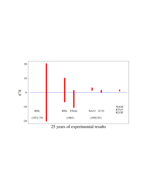
FIG. 1.: 25 years of experiments on $\varepsilon^{\prime}/\varepsilon$ (in units of $10^{-3}$). The last mark on the right, at the average central value of the 1992-93 experiments, shows the experimental precision expected in the forthcoming years.

As it shown in Fig. 1, the experimental error in the determination of this quantity has been dramatically reduced over the years from $10^{-2}$ in the 70’s [Holder:1972aa, Banner:1972aa, Christenson:1979tu, Christenson:1979tt] to $3.5\times 10^{-3}$ in 1985 [Black:1985vj, Bernstein:1985vk] and to roughly $7\times 10^{-4}$ in the last run of experiments in 1992 at CERN and FNAL that obtained respectively [Barr:1993rx, Gibbons:1997fw]

$$\mathop{\mbox{Re}}\>\varepsilon^{\prime}/\varepsilon = (23\pm 3.6\pm 5.4)\times 10^{-4}\;\mbox{(NA31)}\;,$$ (23)

$$\mathop{\mbox{Re}}\>\varepsilon^{\prime}/\varepsilon = (7.4\pm 5.2\pm 2.9)\times 10^{-4}\;\mbox{(E731)}\;,$$ (24)

where the first error is statistical and the second one systematic. As the reader can see, the agreement between the two experiments is within two standard deviations. Moreover, only the CERN result is definitely different from zero.

Before the end of 1999 the new FNAL (E832-KTeV) [Odell:1997ktev] and CERN (NA48) [Holder:1997na48] experiments should provide data with a precision of $(1\div 2)\times 10^{-4}$ and hopefully settle the issue of whether $\varepsilon^{\prime}/\varepsilon$ is or is not zero. Results of the same precision should also be achieved at DA$\Phi$NE (KLOE) [Patera:1997dafne], the Frascati $\Phi$-factory. For a detailed account of the experimental setups and a critical discussion of the issues involved see the review article by [Winstein:1993sx].

From the theoretical point of view, the prediction of the value of $\varepsilon^{\prime}/\varepsilon$ has gone through almost twenty years of increasingly more accurate analyses. By the end of the 70’s, it had been recognized that within the standard model with three generations of quarks, direct $CP$ violation is natural and therefore the model itself is distinguishable from the superweak model. This understanding was the result of an intensive work leading to the identification of the dominant operators responsible for the transition, the so-called penguin operators, and the role played by QCD in their generation [Vainshtein:1975sv, Vainshtein:1977sc]. Typical estimates during this period gave $\varepsilon^{\prime}/\varepsilon$ $\sim 10^{-3}-10^{-2}$ [Ellis:1976fn, Ellis:1977uk, Gilman:1979bc, Gilman:1979wm].

The next step came in the 80’s as the gluon penguin operators above were joined by the electromagnetic operators together with other isospin breaking corrections [Bijnens:1984ye, Donoghue:1986nm, Buras:1987wc, Lusignoli:1989fz]. It was then recognized that these contributions tend to make $\varepsilon^{\prime}$ smaller because they have the opposite sign compared to the gluonic penguin contributions. This part of the computation became particularly critical when by the end of the decade it was realized that the increasingly large mass of the $t$ quark would lead to an increasingly large contribution of the electroweak penguins [Flynn:1989iu, Buchalla:1990we, Paschos:1991as, Lusignoli:1992bm]. This meant a potentially vanishing value for $\varepsilon^{\prime}/\varepsilon$ because of the destructive interference between the two contributions.

By the 90’s the entire subject was mature for a systematic exploration as the short-distance part was brought under control by the next-to-leading order (NLO) determination of the Wilson coefficients of all relevant operators [Buras:1992jm, Buras:1993zv, Buras:1993tc, Buras:1993dy, Ciuchini:1993tj, Ciuchini:1994vr]. This theoretical achievement together with the discovery of the $t$ quark (and the determination of its mass [Barnett:1996hr]) removed two of the largest sources of uncertainty in the prediction. At the same time, independent efforts were brought to bear on the matrix elements estimate. All combined improvements made possible the current predictions of the value of $\varepsilon^{\prime}/\varepsilon$ within the standard model [Heinrich:1992en, Paschos:1996, Buras:1993dy, Buras:1996dq, Ciuchini:1993tj, Ciuchini:1995cd, Ciuchini:1997kd, Bertolini:1996tp, Bertolini:1997nf] that we are to going to review.

2 Outline

The analysis of $\varepsilon^{\prime}/\varepsilon$ can be divided into the short-distance (perturbative) part and the long-distance (mainly non-perturbative) part. As already mentioned, the short-distance part is by now known at the NLO level and is therefore under control. This part of the computation is briefly reviewed in the next section. The long-distance component has been studied by a variety of approaches—lattice QCD, phenomenological estimates and QCD-like models—all of which are eventually combined with chiral perturbation theory. As the long-distance part is the most uncertain, we will spend most of the review on that issue. Section II and III set the common ground on which all approaches are based. Section IV reviews the various determinations of the hadronic matrix elements. After a brief detour, in section V, to determine the relevant CKM matrix elements, in sections VI and VII we bring all elements together to discuss some simple models. We then summarize the current theoretical predictions in the standard model and comment on the issue of new physics.

For a broader view on $CP$ violation which complements the present review, especially in the attention to the experimental issues, the reader is encouraged to consult the article previously published in this journal [Winstein:1993sx].

II The Quark Effective Lagrangian and the NLO Wilson Coefficients

The study of kaon decays within the standard model is made complicated by the huge scale differences involved. Energies as far apart as the mass of the $t$ quark and the mass of the pion must be included. The most satisfactory framework for dealing with physical systems defined across different energy scales is that of effective theories [Weinberg:1980wa, Georgi:1984zz]. The transition amplitudes of an effective theory are assumed to be factorizable in high- and low-energy parts. The degrees of freedom at the higher scales are step-by-step integrated out, retaining only the effective operators made of the lighter degrees of freedom. The short-distance physics, obtained from integrating out the heavy scales, is encoded in the Wilson coefficients that multiply the effective operators. Their evolution with the energy scale is described by the renormalization group equations [Wilson:1971ag].

Figure 2 shows the typical diagrams that in the standard model generate the operators of the effective $\Delta S=1$ Lagrangian.

FIG. 2.: Standard model contributions to the matching of the quark operators in the effective flavor-changing Lagrangian.

The $\Delta S=1$ quark effective lagrangian at a scale $\mu<m_{c}$ can be written [Shifman:1977tn, Gilman:1979bc, Bijnens:1984ye, Lusignoli:1989fz] as

$${\cal L}_{W}=-\sum_{i}C_{i}(\mu)\;Q_{i}(\mu)\;,$$ (25)

where

$$C_{i}(\mu)=\frac{G_{F}}{\sqrt{2}}V_{ud}\,V^{*}_{us}\Bigl{[}z_{i}(\mu)+\tau\ y_{i}(\mu)\Bigr{]}\;.$$ (26)

Here $G_{F}$ if the Fermi coupling, the functions $z_{i}(\mu)$ and $y_{i}(\mu)$ are the Wilson coefficients and $V_{ij}$ the CKM matrix elements; $\tau=-V_{td}V_{ts}^{*}/V_{ud}V_{us}^{*}$. According to the standard parameterization of the CKM matrix, in order to determine $\varepsilon^{\prime}/\varepsilon$, we only need to consider the $y_{i}(\mu)$ components, which control the $CP$-violating part of the Lagrangian. The coefficients $y_{i}(\mu)$, and $z_{i}(\mu)$ contains all the dependence of short-distance physics, and depend on the $t,W,b,c$ masses, the intrinsic QCD scale $\Lambda_{\rm QCD}$ and the renormalization scale $\mu$.

The $Q_{i}$ are the effective four-quark operators obtained in the standard model by integrating out the vector bosons and the heavy quarks $t,\,b$ and $c$. A convenient and by now standard basis includes the following ten operators:

$$\begin{array}[]{rcl}Q_{1}&=&\left(\overline{s}_{\alpha}u_{\beta}\right)_{\rm V-A}\left(\overline{u}_{\beta}d_{\alpha}\right)_{\rm V-A}\,,\\[4.30554pt] Q_{2}&=&\left(\overline{s}u\right)_{\rm V-A}\left(\overline{u}d\right)_{\rm V-A}\,,\\[4.30554pt] Q_{3,5}&=&\left(\overline{s}d\right)_{\rm V-A}\sum_{q}\left(\overline{q}q\right)_{\rm V\mp A}\,,\\[4.30554pt] Q_{4,6}&=&\left(\overline{s}_{\alpha}d_{\beta}\right)_{\rm V-A}\sum_{q}(\overline{q}_{\beta}q_{\alpha})_{\rm V\mp A}\,,\\[4.30554pt] Q_{7,9}&=&\frac{3}{2}\left(\overline{s}d\right)_{\rm V-A}\sum_{q}\hat{e}_{q}\left(\overline{q}q\right)_{\rm V\pm A}\,,\\[4.30554pt] Q_{8,10}&=&\frac{3}{2}\left(\overline{s}_{\alpha}d_{\beta}\right)_{\rm V-A}\sum_{q}\hat{e}_{q}(\overline{q}_{\beta}q_{\alpha})_{\rm V\pm A}\,,\end{array}$$ (27)

where $\alpha$, $\beta$ denote color indices ($\alpha,\beta=1,\ldots,N_{c}$) and $\hat{e}_{q}$ are the quark charges ($\hat{e}_{u}=2/3$, $\hat{e}_{d}=\hat{e}_{s}=-1/3$). Color indices for the color singlet operators are omitted. The labels $(V\pm A)$ refer to the Dirac structure $\gamma_{\mu}(1\pm\gamma_{5})$.

The various operators originate from different diagrams of the fundamental theory. First, at the tree level, we only have the current-current operator $Q_{2}$ induced by $W$-exchange. Switching on QCD, a one-loop correction to $W$-exchange (like in Fig. 2b,c) will induce $Q_{1}$. Furthermore, QCD through the penguin loop (Fig. 2d) induces the gluon penguin operators $Q_{3-6}$. The gluon penguin contribution is split in four components because of the splitting of the gluonic coupling into a right- and a left-handed part and the use of the $SU(N_{c})$ relation

$$2\ T^{a}_{\alpha\delta}T^{a}_{\gamma\beta}=\delta_{\alpha\beta}\delta_{\gamma\delta}-\frac{1}{N_{c}}\delta_{\alpha\delta}\delta_{\gamma\beta}\ ,$$ (28)

where $N_{c}$ is the number of colors, $a=1,\ ...,\ N_{c}^{2}-1$ and $T^{a}$ are the properly normalized $SU(N_{c})$ generators, $\mathop{\mbox{Tr}}T^{a}T^{b}=1/2\ \delta^{ab}$, in the fundamental representation. Electroweak loop diagrams—where the penguin gluon is replaced by a photon or a $Z$-boson and also box-like diagrams—induce $Q_{7,9}$ and also a part of $Q_{3}$. The operators $Q_{8,10}$ are induced by the QCD renormalization of the electroweak loop operators $Q_{7,9}$.

Even though the operators in eq. (27) are not all independent, this basis is of particular interest for any numerical analysis because it is that employed for the calculation of the Wilson coefficients to the NLO order in $\alpha_{s}$ and $\alpha_{e}$ [Buras:1992jm, Buras:1993zv, Buras:1993tc, Buras:1993dy, Ciuchini:1993tj, Ciuchini:1994vr] and we will use it throughout.

Anticipating our discussion, the pie chart in Fig. 3 shows pictorially the relative importance of the operators in eq. (27) in the final determination of the value of $\varepsilon^{\prime}/\varepsilon$ , as obtained in the vacuum saturation approximation to the hadronic matrix elements. In particular, Fig. 3 shows the crucial competition between gluonic and electroweak penguins in the determination of the value of $\varepsilon^{\prime}/\varepsilon$ . Such a destructive interference might accidentally lead to a vanishing $\varepsilon^{\prime}/\varepsilon$ even in the presence of a source of direct $CP$ violation. This feature adds to the theoretical challenge of predicting $\varepsilon^{\prime}/\varepsilon$ with the required accuracy.

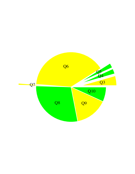
FIG. 3.: Relative contributions to $\varepsilon^{\prime}/\varepsilon$ of the operators in eq. (27). Operators giving a (negative) positive contribution are depicted in (dark) light gray. All matrix elements are taken in the vacuum saturation approximation. The operators $Q_{8}$ and $Q_{10}$ are generated by QCD and do not receive contributions from the one-loop matching.

While there exist other possible operators in addition to those listed in eq. (27), they are numerically irrelevant within the standard model. For instance, the two operators

$$Q_{11}=\frac{g_{s}}{8\pi^{2}}\>\bar{s}\>\left[m_{d}R+m_{s}L\right]\>\sigma\cdot G\>d\;\quad\quad\mbox{and}\quad\quad Q_{12}=\frac{e}{8\pi^{2}}\>\bar{s}\>\left[m_{d}R+m_{s}L\right]\>\sigma\cdot F\>d\;,$$ (29)

where $R=\left(1+\gamma_{5}\right)/2$ and $L=\left(1-\gamma_{5}\right)/2$, are present. These operators are induced by gluon and photon penguins with a free gluon (photon) leg. The matrix elements of these operators give a vanishingly small contribution to $K\to\pi\pi$ decays [Bertolini:1995qk, Bertolini:1997ir].

In table I we summarize in a synthetic way the diagrammatic origin of the contributions to the various Wilson coefficients when considering the one-loop matching of the quark effective lagrangian with the full electroweak theory.

TABLE I.: Contributions to the one-loop matching of the $\Delta S=1$ Wilson coefficients at $\mu=m_{W}$. The notation refers to that of eq. (25) and Fig. 2. Non-vanishing contributions to $C_{8}$ and $C_{10}$ arise via the QCD renormalization of the operators $Q_{7}$ and $Q_{9}$, respectively.

$\mu=m_{W}$	$C_{1}$	$C_{2}$	$C_{3}$	$C_{4}$	$C_{5}$	$C_{6}$	$C_{7}$	$C_{8}$	$C_{9}$	$C_{10}$
Tree		$\surd$
Tree + $g$	$\surd$	$\surd$
Tree + $\gamma$		$\surd$
${\cal P}_{g}$			$\surd$	$\surd$	$\surd$	$\surd$
${\cal P}_{\gamma}$							$\surd$		$\surd$
${\cal P}_{Z}$			$\surd$				$\surd$		$\surd$
${\cal B}$			$\surd$						$\surd$

Having established the operator basis, a full two-loop calculation (up to $\alpha_{s}^{2}$ and $\alpha_{s}\alpha_{em}$) of the quark operator anomalous dimensions is performed. This calculation allows us via renormalization group methods to evaluate the Wilson coefficients at the typical scale of the process, thus resumming (perturbatively) potentially large logarithmic effects to a few 10% uncertainty. As already mentioned, the size of the Wilson coefficients at the hadronic scale (of the order of 1 GeV) depends on $\alpha_{s}$ and the threshold masses $m_{t}$, $m_{W}$, $m_{b}$ and $m_{c}$. The top quark mass dependence enters in the penguin coefficients $y_{i}(\mu)$ via the initial matching conditions for the renormalization group equations.

Small differences in the short-distance input parameters are present in the various treatment in the literature. In order to give the reader an idea of the ranges used, we list below some of the values.

The most recent determination of the running strong coupling in the $\overline{MS}$ scheme is [Barnett:1996hr]

$$\alpha_{s}(m_{Z})=0.119\pm 0.002\,,$$ (30)

which at the NLO corresponds to

$$\Lambda^{(4)}_{\rm QCD}=340\pm 40\>\mbox{MeV}\,.$$ (31)

For $m_{t}$ we take the value [Tipton:1996aa]

$$m_{t}^{\rm pole}=175\pm 6\>\>\mbox{GeV}\,.$$ (32)

The knowledge of the top quark mass is one important ingredient in the reduced uncertainty of the recent estimates of $\varepsilon^{\prime}/\varepsilon$ .

The relation between the pole mass $M$ and the $\overline{\rm MS}$ running mass $m(\mu)$ is given at one loop in QCD by

$$m(M)\ =\ {M(q^{2}=M^{2})}\ {\left[1-\frac{4}{3}\frac{\alpha_{s}(M)}{\pi}\right]}\ \ ,$$ (33)

For the running top quark mass, in the range of $\alpha_{s}$ considered, we then obtain

$$m_{t}(m_{t})\simeq 167\pm 6\>\>\mbox{GeV}\;,$$ (34)

which, using the one-loop running, corresponds to

$$m_{t}(m_{W})\simeq 177\pm 7\>\>\mbox{GeV}\;,$$ (35)

which is the value to be used as input at the $m_{W}$ scale for the NLO evolution of the Wilson coefficients. In eq. (35) we have averaged over the range of $\Lambda^{(4)}_{\rm QCD}$ given in eq. (31).

The use of the running top mass in the initial matching of the Wilson coefficients softens the matching scale dependence present in the LO analysis. By taking $\mu=m_{t}^{\rm pole}$ as the starting matching scale in place of $m_{W}$, and using correspondingly $m_{t}(m_{t})$, the NLO Wilson coefficients of the electroweak and gluon penguins at $\mu\simeq 1$ GeV, remain stable up to the 10% percent level.

For $m_{b}$ we have the mass range [Barnett:1996hr]

$$m_{b}^{\rm pole}=4.5\div 4.9\>\>\mbox{GeV}\;,$$ (36)

which corresponds to

$$m_{b}(m_{b})=4.1\div 4.5\>\>\mbox{GeV}\;.$$ (37)

Analogously, for $m_{c}$ one has

$$m_{c}^{\rm pole}=1.2\div 1.9\>\>\mbox{GeV}\;,$$ (38)

which corresponds to

$$m_{c}(m_{c})=1.0\div 1.6\>\>\mbox{GeV}\;,$$ (39)

Values within the $\overline{MS}$ ranges have to be used as the quark thresholds in evolving the Wilson coefficients down to the low-energy scale where the matching with the hadronic matrix elements is to be performed.

In choosing the quark mass thresholds one should bear in mind that varying $m_{b}^{\rm pole}$ within the given range affects the final values of the Wilson coefficients only at the percent level, while varying the charm pole mass in the whole range given may affects the real part of the gluon penguin coefficients up to the 20% level. We will take $m_{b}(m_{b})=4.4\>\>\mbox{GeV}$ and $m_{c}(m_{c})=1.4\>\>\mbox{GeV}$.

TABLE II.: The $\Delta S=1$ NLO Wilson coefficients relevant for CP violation are given at $\mu=1.0$ GeV for $m_{t}(m_{W})=177$ GeV, which corresponds to $m_{t}^{pole}=175$ GeV, ($\alpha=1/128$). In addition one has $y_{1,2}(\mu)=0$.

$\Lambda_{QCD}^{(4)}$	300 MeV		340 MeV		380 MeV
	HV	NDR	HV	NDR	HV	NDR
$y_{3}$	$0.0341$	$0.0298$	$0.0378$	$0.0326$	$0.0420$	$0.0356$
$y_{4}$	$-0.0558$	$-0.0530$	$-0.0597$	$-0.0564$	$-0.0639$	$-0.0597$
$y_{5}$	$0.0149$	$0.000687$	$0.0160$	$-0.00204$	$0.0173$	$-0.00581$
$y_{6}$	$-0.0883$	$-0.100$	$-0.0994$	$-0.115$	$-0.113$	$-0.133$
$y_{7}/\alpha$	$-0.0202$	$-0.0210$	$-0.0195$	$-0.0209$	$-0.0188$	$-0.0209$
$y_{8}/\alpha$	$0.184$	$0.169$	$0.209$	$0.192$	$0.240$	$0.220$
$y_{9}/\alpha$	$-1.70$	$-1.70$	$-1.75$	$-1.74$	$-1.80$	$-1.80$
$y_{10}/\alpha$	$0.735$	$0.722$	$0.806$	$0.790$	$0.885$	$0.867$

In table II we report the numerical values of the NLO Wilson coefficients relevant for $CP$ violation in $\Delta S=1$ processes. The coefficients $y_{i}(\mu)$ are given at the scale $\mu=1$ GeV and are dependent on the choice of the $\gamma_{5}$ scheme in dimensional regularization. The values in the table refer to two commonly used schemes, namely the naive dimensional regularization (NDR), in which $\gamma_{5}$ anticommutes with the Dirac matrices in $d$ dimensions, and the t’ Hooft-Veltman scheme (HV) ['tHooft:1972fi], in which they anticommute only in four dimensions. The latter prescription has been shown to be a consistent formulation of dimensional regularization in the presence of chiral couplings [Breitenlohner:1977te]. A consistent calculation of the hadronic matrix elements should match the unphysical scale and scheme dependence of the Wilson coefficients so as to produce a stable amplitude at the given order in perturbation theory. We will return on this issue in Sect IV when discussing the various approaches to the long distance part of the calculation.

The case of the $\Delta S=2$ theory is treated along similar lines. The effective $\Delta S=2$ quark lagrangian at scales $\mu<m_{c}$ is given by

$${\cal L}_{\Delta S=2}=-C_{2S}(\mu)\;Q_{S2}(\mu)\;,$$ (40)

where

$$C_{2S}(\mu)=\frac{G_{F}^{2}m_{W}^{2}}{4\pi^{2}}\left[\lambda_{c}^{2}\eta_{1}S(x_{c})+\lambda_{t}^{2}\eta_{2}S(x_{t})+2\lambda_{c}\lambda_{t}\eta_{3}S(x_{c},x_{t})\right]b(\mu)$$ (41)

where $\lambda_{j}=V_{jd}V_{js}^{*}$, $x_{i}=m_{i}^{2}/m_{W}^{2}$. We denote by $Q_{S2}$ the $\Delta S=2$ local four quark operator

$$Q_{S2}=(\bar{s}_{L}\gamma^{\mu}d_{L})(\bar{s}_{L}\gamma_{\mu}d_{L})\,,$$ (42)

which is the only local operator of dimension six in the standard model.

The integration of the electroweak loops leads to the Inami-Lim functions [Inami:1981fz] $S(x)$ and $S(x_{c},x_{t})$, the exact expressions of which can be found in the reference quoted, depend on the masses of the charm and top quarks and describe the $\Delta S=2$ transition amplitude in the absence of strong interactions.

The short-distance QCD corrections are encoded in the coefficients $\eta_{1}$, $\eta_{2}$ and $\eta_{3}$ with a common scale-dependent factor $b(\mu)$ factorized out. They are functions of the heavy quarks masses and of the scale parameter $\Lambda_{\rm QCD}$. These QCD corrections are available at the NLO [Buras:1990fn, Herrlich:1994yv, Herrlich:1995hh, Herrlich:1996vf] in the strong and electromagnetic couplings.

The scale-dependent common factor of the short-distance corrections is given by

$$b(\mu)=\left[\alpha_{s}\left(\mu\right)\right]^{-2/9}\left(1-J_{3}\frac{\alpha_{s}\left(\mu\right)}{4\pi}\right)\,,$$ (43)

where $J_{3}$ depends on the $\gamma_{5}$-scheme used in the regularization. The NDR and HV scheme yield, respectively:

$$J_{3}^{\rm NDR}=-\frac{307}{162}\quad\quad\mbox{and}\quad\quad J_{3}^{\rm HV}=-\frac{91}{162}\,.$$ (44)

All the other numerical inputs can be taken as in the $\Delta S=1$ case.

III Chiral Perturbation Theory

Quarks are the fundamental hadronic matter. However, the particles we observe are those built out of them: baryons and mesons. In the sector of the lowest mass pseudoscalar mesons (the would-be Goldstone bosons: $\pi$, $K$ and $\eta$), the interactions can be described in terms of an effective theory, the chiral lagrangian, that includes only these states. The chiral lagrangian and chiral perturbation theory [Weinberg:1979kz, Gasser:1985gg, Gasser:1984yg] provide a faithful representation of this sector of the standard model after the quark and gluon degrees of freedom have been integrated out. The form of this effective field theory and all its possible terms are determined by $SU_{L}(3)\times SU_{R}(3)$ chiral invariance and Lorentz invariance. The parts of the lagrangian which explicitly break chiral invariance are introduced in terms of the quark mass matrix $\cal{M}$.

The strong chiral lagrangian is completely fixed to the leading order in momenta by symmetry requirements and the Goldstone boson’s decay constant $f$:

$${\cal L}_{\rm strong}^{(2)}=\frac{f^{2}}{4}\mathop{\mbox{Tr}}\left(D_{\mu}\Sigma D^{\mu}\Sigma^{{\dagger}}\right)+\frac{f^{2}}{2}B_{0}\mathop{\mbox{Tr}}\left({\cal M}\Sigma^{{\dagger}}+\Sigma{\cal M}^{{\dagger}}\right)\,,$$ (45)

where ${\cal M}=\mbox{diag}[m_{u},m_{d},m_{s}]$ and $B_{0}$ is given by $\langle\bar{q}_{i}q_{j}\rangle=-f^{2}B_{0}\delta_{ij}$, with

$$\langle\bar{q}q\rangle=-\frac{f^{2}m_{K}^{2}}{m_{s}+m_{d}}=-\frac{f^{2}m_{\pi}^{2}}{m_{u}+m_{d}}\;,$$ (46)

according to PCAC in the limit of $SU(3)$ flavor symmetry ($f_{K}=f_{\pi}\equiv f$). The $SU_{L}(3)\times SU_{R}(3)$ field

$$\Sigma\equiv\exp\left(\frac{2i}{f}\,\Pi(x)\right)$$ (47)

contains the pseudoscalar octet:

$$\Pi(x)=\frac{1}{2}\sum_{a=1}^{8}\lambda^{a}\pi^{a}(x)=\frac{1}{\sqrt{2}}\left[\begin{array}[]{ccc}\tilde{\pi}^{0}&\pi^{+}&K^{+}\\ \pi^{-}&-\bar{\pi}^{0}&K^{0}\\ K^{-}&\bar{K}^{0}&\tilde{\pi}^{8}\end{array}\right]\,,$$ (48)

where

$$\tilde{\pi}^{0}=\frac{1}{\sqrt{2}}\pi^{0}+\frac{1}{\sqrt{6}}\eta_{8}\,,\qquad\bar{\pi}^{0}=\frac{1}{\sqrt{2}}\pi^{0}-\frac{1}{\sqrt{6}}\eta_{8}\,,\qquad\tilde{\pi}^{8}=-\frac{2}{\sqrt{6}}\eta_{8}\,.$$ (49)

The coupling $f$ is, to lowest order, identified with the pion decay constant $f_{\pi}$ (and equal to $f_{K}$ before chiral loops are introduced); it defines a characteristic scale

$$\Lambda_{\chi}\equiv 2\pi\sqrt{6/N_{c}}\,f\,\simeq 0.8\>\mbox{GeV}\,,$$ (50)

typical of the vector meson masses induced by the spontaneous breaking of chiral symmetry. When the matrix $\Sigma$ is expanded in powers of $f^{-1}$, the zeroth order term is the free Klein-Gordon lagrangian for the pseudoscalar particles.

Under the action of the elements $V_{R}$ and $V_{L}$ of the chiral group $SU_{R}(3)\times SU_{L}(3)$, $\Sigma$ transforms linearly:

$$\Sigma^{\prime}=V_{R}\Sigma V_{L}^{{\dagger}}\;,$$ (51)

with the quark fields transforming as

$$q_{L}^{\prime}=V_{L}\,q_{L}\qquad\mbox{and}\qquad q_{R}^{\prime}=V_{R}\,q_{R}\;,$$ (52)

and accordingly for the conjugated fields.

Quark operators are represented in this language in terms of the effective field $\Sigma$ and its derivatives. For instance, at the leading order, the quark currents are given by

$$\bar{q}^{j}_{L}\gamma_{\mu}q^{i}_{L} \to -i\frac{f^{2}}{2}\left(\Sigma^{{\dagger}}D_{\mu}\Sigma\right)_{ij}\,,$$ (53)

$$\bar{q}^{j}_{R}\gamma_{\mu}q^{i}_{R} \to -i\frac{f^{2}}{2}\left(\Sigma D_{\mu}\Sigma^{{\dagger}}\right)_{ij}\,,$$ (54)

while the quark densities can be written at $O(p^{2})$ as

$$\bar{q}^{j}_{L}q^{i}_{R} \to -2B_{0}\left[\frac{f^{2}}{4}\Sigma+L_{5}\ \Sigma D_{\mu}\Sigma^{{\dagger}}D^{\mu}\Sigma+4B_{0}L_{8}\ \Sigma{\cal M}^{\dagger}\ \Sigma\right]_{ij}\,,$$ (55)

$$\bar{q}^{j}_{R}q^{i}_{L} \to -2B_{0}\left[\frac{f^{2}}{4}\Sigma^{\dagger}+L_{5}\ \Sigma^{\dagger}D_{\mu}\Sigma D^{\mu}\Sigma^{{\dagger}}+4B_{0}L_{8}\Sigma^{{\dagger}}{\cal M}\ \Sigma^{{\dagger}}\right]_{ij}\,,$$ (56)

where $L_{5,8}$ are coefficients which belong to the $O(p^{4})$ chiral lagrangian. To the next-to-leading order in the momenta, in addition to the leading order chiral lagrangian (45), there are ten chiral terms and thereby ten coefficients $L_{i}$ to be determined [Gasser:1984yg, Gasser:1985gg] either experimentally or by means of some model. As we shall see, some of them play an important role in the physics of $\varepsilon^{\prime}/\varepsilon$ . As an example, we display the $L_{5}$ and $L_{8}$ terms in ${\cal L}_{\rm strong}^{(4)}$ which appear in eq. (56) and govern much of the penguin physics:

$$L_{5}\,B_{0}\,\mathop{\mbox{Tr}}\left[D_{\mu}\Sigma D^{\mu}\Sigma^{{\dagger}}\left({\cal M}\Sigma^{{\dagger}}+\Sigma{\cal M}^{{\dagger}}\right)\right]\quad\mbox{and}\quad L_{8}\,B_{0}\,\mathop{\mbox{Tr}}\left[{\cal M}^{{\dagger}}\Sigma{\cal M}^{{\dagger}}\Sigma+{\cal M}\Sigma^{{\dagger}}{\cal M}\Sigma^{{\dagger}}\right]\,.$$ (57)

A The Weak Chiral Lagrangian

We can write the most general expression for the $\Delta S=1$ chiral lagrangian in accordance with the $SU(3)_{L}\times SU(3)_{R}$ symmetry, involving unknown constants of order $G_{F}$. This is done order by order in the chiral expansion. Typical terms to $O(p^{2})$ are obtained by inserting appropriate combinations of Gell-Mann matrices into the strong lagrangian. The corresponding chiral coefficients must then be determined by means of some model or by comparison to the experimental data.

We find it convenient to write the $\Delta S=1$ chiral lagrangian at $O(p^{2})$ in terms of the following eight terms, of which seven are linearly independent:

$${\cal L}^{(2)}_{\Delta S=1}= G_{LR}^{(0)}(Q_{7,8})\mathop{\mbox{Tr}}\left(\lambda^{3}_{2}\Sigma^{{\dagger}}\lambda^{1}_{1}\Sigma\right)$$ (58)

$$+ G_{LR}^{(m)}(Q_{7,8})\ \left[\mathop{\mbox{Tr}}\left(\lambda^{3}_{2}\Sigma^{\dagger}\lambda_{1}^{1}\Sigma{\cal M}^{\dagger}\Sigma\right)+\mathop{\mbox{Tr}}\left(\lambda_{1}^{1}\Sigma\lambda^{3}_{2}\Sigma^{\dagger}{\cal M}\Sigma^{\dagger}\right)\right]$$ (59)

$$+ G_{\underline{8}}(Q_{3-10})\mathop{\mbox{Tr}}\left(\lambda^{3}_{2}D_{\mu}\Sigma^{{\dagger}}D^{\mu}\Sigma\right)$$ (60)

$$+ G_{LL}^{a}(Q_{1,2,9,10})\,\mathop{\mbox{Tr}}\left(\lambda^{3}_{1}\Sigma^{{\dagger}}D_{\mu}\Sigma\right)\mathop{\mbox{Tr}}\left(\lambda^{1}_{2}\Sigma^{{\dagger}}D^{\mu}\Sigma\right)$$ (61)

$$+ G_{LL}^{b}(Q_{1,2,9,10})\,\mathop{\mbox{Tr}}\left(\lambda^{3}_{2}\Sigma^{{\dagger}}D_{\mu}\Sigma\right)\mathop{\mbox{Tr}}\left(\lambda^{1}_{1}\Sigma^{{\dagger}}D^{\mu}\Sigma\right)$$ (62)

$$+ G_{LR}^{a}(Q_{7,8})\,\mathop{\mbox{Tr}}\left(\lambda^{3}_{2}D_{\mu}\Sigma\lambda^{1}_{1}D^{\mu}\Sigma^{{\dagger}}\right)$$ (63)

$$+ G_{LR}^{b}(Q_{7,8})\,\mathop{\mbox{Tr}}\left(\lambda^{3}_{2}\Sigma^{{\dagger}}D_{\mu}\Sigma\right)\mathop{\mbox{Tr}}\left(\lambda^{1}_{1}\Sigma D^{\mu}\Sigma^{{\dagger}}\right)$$ (64)

$$+ G_{LR}^{c}(Q_{7,8})\left[\mathop{\mbox{Tr}}\left(\lambda^{3}_{1}\Sigma\right)\mathop{\mbox{Tr}}\left(\lambda^{1}_{2}D_{\mu}\Sigma^{{\dagger}}D^{\mu}\Sigma\ \Sigma^{{\dagger}}\right)+\mathop{\mbox{Tr}}\left(\lambda^{3}_{1}D_{\mu}\Sigma D^{\mu}\Sigma^{{\dagger}}\ \Sigma\right)\mathop{\mbox{Tr}}\left(\lambda^{1}_{2}\Sigma^{{\dagger}}\right)\right]\,,$$ (65)

where $\lambda^{i}_{j}$ are combinations of Gell-Mann $SU(3)$ matrices defined by $(\lambda^{i}_{j})_{lk}=\delta_{il}\delta_{jk}$ and $\Sigma$ is defined in eq. (47). The covariant derivatives in eq. (65) are taken with respect to the external gauge fields whenever they are present. Other terms are possible, but they can be reduced to these by means of trace identities.

The non-standard form and notation of eq. (65) is chosen to remind us of the flavor and chiral structure of the effective four-quark operators which are represented by the various terms. In particular, in $G_{\underline{8}}$ we collect the $(\underline{8}_{L}\times\underline{1}_{R})$ part of the interaction which is induced by the gluonic penguins and by the analogous components of the electroweak operators $Q_{7-10}$. The two terms proportional to $G_{LL}^{a}$ and $G_{LL}^{b}$ are an admixture of the $(\underline{27}_{L}\times\underline{1}_{R})$ and the $(\underline{8}_{L}\times\underline{1}_{R})$ part of the interactions induced by the left-handed current-current operators $Q_{1,2,9,10}$. The term proportional to $G_{LR}^{(0)}$ is the constant (non-derivative) $O(p^{0})$ part arising from the isospin violating $(\underline{8}_{L}\times\underline{8}_{R})$ electroweak operators. The $O(p^{2})$ corrections to $G_{LR}^{(0)}$ are the quark mass term proportional to $G_{LR}^{(m)}$ (related to $L_{8}$), the momentum corrections proportional to $G_{LR}^{c}$ (related to $L_{5}$) and $G_{LR}^{a,b}$. One may verify that $G_{LR}^{(m)}$ and $G_{LR}^{c}$ can be obtained by multiplying the bosonized expression of a left- and a right-handed quark density (in a manner similar to $Q_{6})$, while $G_{LR}^{b}$ is obtained as the product of a left- and a right-handed quark current. It is therefore natural to call these terms factorizable (although $G_{LR}^{b}$ has a non-factorizable contribution). The term $G_{LR}^{a}$ is, however, genuinely non-factorizable [Fabbrichesi:1996iz].

The terms proportional to $G_{\underline{8}}$, $G^{a}_{LL}$ and $G^{b}_{LL}$ have been studied in the literature [Cronin:1967jq, Pich:1991mw, Bijnens:1993uz, Ecker:1993de] in the framework of chiral perturbation theory. The three terms are not independent. Those proportional to $G^{a}_{LL}$ and $G^{b}_{LL}$ can be written in terms of the $\underline{8}$ and $\underline{27}$ $SU(3)_{L}$ components as follows:

$${\cal L}_{\underline{27}}=G_{\underline{27}}(Q_{i})\>\left[\frac{2}{3}\,\mathop{\mbox{Tr}}\left(\lambda^{3}_{1}\Sigma^{{\dagger}}D^{\mu}\Sigma\right)\mathop{\mbox{Tr}}\left(\lambda^{1}_{2}\Sigma^{{\dagger}}D_{\mu}\Sigma\right)+\>\mathop{\mbox{Tr}}\left(\lambda^{3}_{2}\Sigma^{{\dagger}}D_{\mu}\Sigma\right)\mathop{\mbox{Tr}}\left(\lambda^{1}_{1}\Sigma^{{\dagger}}D^{\mu}\Sigma\right)\right]\,,$$ (66)

which transforms as $(\underline{27}_{L}\times\underline{1}_{R})$, and

$${\cal L}_{\underline{8}}=G_{\underline{8}}(Q_{i})\>\left[\mathop{\mbox{Tr}}\left(\lambda^{3}_{1}\Sigma^{{\dagger}}D^{\mu}\Sigma\right)\mathop{\mbox{Tr}}\left(\lambda^{1}_{2}\Sigma^{{\dagger}}D_{\mu}\Sigma\right)-\>\mathop{\mbox{Tr}}\left(\lambda^{3}_{2}\Sigma^{{\dagger}}D_{\mu}\Sigma\right)\mathop{\mbox{Tr}}\left(\lambda^{1}_{1}\Sigma^{{\dagger}}D^{\mu}\Sigma\right)\right]\,,$$ (67)

which transforms as $(\underline{8}_{L}\times\underline{1}_{R})$. We prefer to keep the $\Delta S=1$ chiral Lagrangian in the form given in eq. (65), which makes the bosonization of each quark operator more transparent, and perform the needed isospin projections at the level of the matrix elements. Equations (66)–(67) provide anyhow the comparison to the standard notation. The chiral coefficients in the two bases are related by

$$G_{\underline{8}}(Q_{i}) = \frac{1}{5}\left[3\>G^{a}_{LL}(Q_{i})-2\>G^{b}_{LL}(Q_{i})\right]$$ (68)

$$G_{\underline{27}}(Q_{i}) = \frac{3}{5}\left[G^{a}_{LL}(Q_{i})+G^{b}_{LL}(Q_{i})\right]\;,$$ (69)

for $i=1,2$. Notice that there is no over-counting of the $\underline{8}_{L}\times\underline{1}_{R}$ contributions to eq. (65) from the operators $Q_{9,10}$ when a consistent prescription like that given in [Antonelli:1996nv] is followed.

Concerning the $(\underline{8}_{L}\times\underline{8}_{R})$ part of the $\Delta S=1$ chiral lagrangian, the constant term was first considered in [Bijnens:1984ye], while its mass and $O(p^{2})$ momentum corrections were first discussed in [Antonelli:1996nv, Bertolini:1997nf].

As an example of the form of the chiral coefficients, we give the determination in the leading order in $1/N_{c}$ of the two most important contributions to $\varepsilon^{\prime}/\varepsilon$ :

$$G_{\underline{8}}(Q_{6})=-24\frac{\langle\bar{q}q\rangle^{2}L_{5}}{f^{2}}\,C_{6}$$ (70)

and

$$G^{(0)}(Q_{8})=-3\langle\bar{q}q\rangle^{2}\,C_{8}\;,$$ (71)

where $C_{6,8}$ are the Wilson coefficients of the operators $Q_{6,8}$ at the matching scale $\mu$.

The $\Delta S=1$ $O(p^{4})$ Lagrangian is much more complicated  [Kambor:1990tz, Esposito-Farese:1991yq, Ecker:1993de, Bijnens:1998mb] but we will not need its explicit form. In fact, only certain combinations of coefficients from the $O(p^{4})$ are required in order to compute the relevant amplitudes to this approximation.

The $\Delta S=2$ weak chiral lagrangian is simpler. At the leading order $O(p^{2})$, the $\Delta S=2$ weak chiral lagrangian is given by only one term:

$${\cal L}^{(2)}_{\Delta S=2}=G(Q_{S2})\mathop{\mbox{Tr}}\left(\lambda^{3}_{2}\Sigma D_{\mu}\Sigma^{{\dagger}}\right)\mathop{\mbox{Tr}}\left(\lambda^{3}_{2}\Sigma D^{\mu}\Sigma^{{\dagger}}\right)\,.$$ (72)

The chiral coefficient is in this case given at the LO in $1/N_{c}$ by

$$G(Q_{S2})=-\frac{f^{4}}{4}\,C_{2S}\,.$$ (73)

IV Hadronic Matrix Elements

The estimate of the hadronic matrix elements must rely on long-distance effects of QCD. It is useful to encode the result of different estimates in terms of the $B_{i}$ parameters that are defined in terms of the matrix elements

$$\langle Q_{i}\rangle_{0,2}\equiv\langle(\pi\pi)_{(I=0,2)}|Q_{i}|K^{0}\rangle$$ (74)

as

$$B_{i}^{(0,2)}\equiv\frac{\mathop{\mbox{Re}}\langle Q_{i}\rangle_{0,2}^{\rm model}}{\langle Q_{i}\rangle_{0,2}^{\rm VSA}}\;,$$ (75)

and give the ratios between hadronic matrix elements in a model and those of the vacuum saturation approximation (VSA). The latter is defined by factorizing the four-quark operators, inserting the vacuum state in all possible manners (Fierzing of the operators included) and by keeping the first non-vanishing term in the momentum expansion of each contribution.

As a typical example, the matrix element of $Q_{6}$ in the factorized version can be written as the product of density matrix elements

$$\langle\pi^{+}\pi^{-}|Q_{6}|K^{0}\rangle = 2\,\langle\pi^{+}|\overline{u}\gamma_{5}d|0\rangle\langle\pi^{-}|\overline{s}u|K^{0}\rangle-2\langle\pi^{+}\pi^{-}|\overline{d}d|0\rangle\langle 0|\overline{s}\gamma_{5}d|K^{0}\rangle$$ (77)

$$+2\,\left[\langle 0|\overline{s}s|0\rangle\,-\,\langle 0|\overline{d}d|0\rangle\right]\,\langle\pi^{+}\pi^{-}|\overline{s}\gamma_{5}d|K^{0}\rangle\,,$$

where the matrix elements like $\langle 0|\,\overline{s}\gamma_{5}u\,|K^{+}\rangle$ and $\langle\pi^{+}|\,\overline{s}d\,|K^{+}\rangle$ are obtained from PCAC and the standard parameterization of the corresponding currents, $\langle 0|\,\overline{s}\gamma^{\mu}\left(1-\gamma_{5}\right)u\,|K^{+}\rangle$ and $\langle\pi^{+}|\,\overline{s}\gamma^{\mu}\left(1-\gamma_{5}\right)u\,|K^{+}\rangle$. In the same way, the left-left currents operators can be written in the factorizable approximation in terms of matrix elements of the currents.

Notice that the definition in eq. (75) neglects the imaginary (absorptive) parts of the hadronic matrix elements. Imaginary and real components, when multiplied by the corresponding short-distance coefficients and summed over the contributing operators, should reproduce the global phase of the amplitude arising from final state interactions. However, some approaches to hadronic matrix elements do not account for absorptive contributions. Therefore, in order to make the discussion of the $B_{i}$ factors of different models as homogeneous as possible, we propose the definition in eq. (75). Consistently with the use of such a definition, extra overall $1/\cos\delta_{0,2}$ factors appear in the $I=0,2$ amplitudes, as discussed in Sect. VI.

A Preliminary Remarks

The $B_{i}$ parameters depend in principle on the renormalization scale $\mu$ and therefore they should be given together with the scale at which they are evaluated.

In this respect, in a truly consistent calculation of the hadronic matrix elements, the cancellation of the unphysical renormalization scale and scheme dependence of the Wilson coefficients should formally be proven order by order in perturbation theory.

The only approach that fully satisfies these requirements is that based on the lattice regularization (discussed in subsection F), where the same theory, namely QCD, is used in both the short- and the long-distance regimes and the matching only involves the different regularization schemes.

The München phenomenological approach (discussed in subsection E) represents a clever attempt to address the problem of a consistent calculation of $\varepsilon^{\prime}/\varepsilon$ in a framework originally based on the $1/N_{c}$ expansion. In this approach one extracts as much information as possible on the hadronic matrix elements by fitting the $\Delta I=1/2$ selection rule at a fixed scale and in a given renormalization scheme. The scale and renormalization scheme stability of physical amplitudes can then be obtained using perturbation theory since the matching scale between short- and long- distance calculations is large enough ($\mu=m_{c}$) to lie inside the perturbative regime. The phenomenological input allows for a direct determination of the current-current matrix elements and indirectly of some of the penguin matrix elements, thus reducing the number of free parameters in the $\Delta S=1$ effective lagrangian. On the other hand, the same fit does not give any information on the actual value (and scheme dependence) of the $B_{6,8}$ parameters at the given scale, which are the most relevant for determining $\varepsilon^{\prime}/\varepsilon$ .

In the Trieste group approach (discussed in subsection G) there is no attempt to prove formally the consistency of the matching along the lines stated above. The matching is done between QCD on the short-distance side and phenomenological models, the $\chi$QM and chiral perturbation theory, on the long-distance side. In the long-distance calculation the scale and renormalization scheme dependences appear naturally. It is then assumed that these unphysical dependences may satisfactorily match those of the short-distance calculation. The fact that this assumption is numerically verified (even beyond expectation), thus giving at the given order of the calculation a stable set of predictions, and that it allows for a complete calculation of all matrix elements in terms of a few basic “non-perturbative” parameters, make this phenomenological analysis valuable. The pattern of contributions which emerges and which leads to a satisfactory reproduction of the $\Delta I=1/2$ rule may be of help in other investigations. The major weakness of the approach is the poor convergence of the chiral expansion at matching scales of the order of the $\rho$ mass or higher, which are required by the reliability of the perturbative strong coupling expansion.

Very recently the Dortmund group (see subsection D) has developed a systematic procedure for matching short- and long-distance calculations, improving both technically and conceptually on the original $1/N_{c}$ approach of [Bardeen:1987uz]. On the other hand, at the present status of the calculation, the scale stability of the matching with the short-distance coefficients is for some of the relevant observables ($\Delta I=1/2$, $3/2$ amplitudes, $\hat{B}_{K}$) quite poor [Hambye:1997dh, Kohler:1997pg].

B The Vacuum Saturation Approximation

According to the discussion above it is clear that there is no theoretical underpinning for the consistency of the VSA; it is a convenient reference frame which is equivalent to retaining terms of $O(1/N_{c})$ in the $1/N_{c}$-expansion to the leading (non-vanishing) order in the momenta for all Fierzed forms of the operators. Its application should in general not be pushed beyond leading order in the strong coupling expansion. On the other hand, we find it useful for illustrative purposes to use the VSA hadronic matrix elements together with NLO Wilson coefficients in order to exhibit some features of the long-distance calculation and allow for a homogeneous comparison with the other estimates. For this purpose we will use in all numerical estimates the Wilson coefficients obtained in the HV scheme and set the matching scale at 1 GeV (see table II).

Some of the relevant VSA hadronic matrix elements depend on parameters that are not precisely known. As a consequence, the knowledge of the $B_{i}$ is not the whole story and, depending on assumptions, different predictions of $\varepsilon^{\prime}/\varepsilon$ may well differ even starting from the same set of $B_{i}$. It is therefore important to define carefully the VSA matrix elements. According to the standard bosonization of currents and densities at $O(p^{2})$ one obtains:

$$\langle Q_{1}\rangle_{0} = \frac{1}{3}X\left[-1+\frac{2}{N_{c}}\right]\;,$$ (78)

$$\langle Q_{1}\rangle_{2} = \frac{\sqrt{2}}{3}X\left[1+\frac{1}{N_{c}}\right]\;,$$ (79)

$$\langle Q_{2}\rangle_{0} = \frac{1}{3}X\left[2-\frac{1}{N_{c}}\right]\;,$$ (80)

$$\langle Q_{2}\rangle_{2} = \frac{\sqrt{2}}{3}X\left[1+\frac{1}{N_{c}}\right]\;,$$ (81)

$$\langle Q_{3}\rangle_{0} = \frac{1}{N_{c}}X\;,$$ (82)

$$\langle Q_{4}\rangle_{0} = X\;,$$ (83)

$$\langle Q_{5}\rangle_{0} = -\frac{16}{N_{c}}\,\frac{\langle\bar{q}q\rangle^{2}L_{5}}{f^{6}}\,X\;,$$ (84)

$$\langle Q_{6}\rangle_{0} = -16\,\frac{\langle\bar{q}q\rangle^{2}L_{5}}{f^{6}}\,X\;,$$ (85)

$$\langle Q_{7}\rangle_{0} = \frac{2\sqrt{3}}{N_{c}}\,\frac{\langle\bar{q}q\rangle^{2}}{f^{3}}+\frac{8}{N_{c}}\,\frac{\langle\bar{q}q\rangle^{2}L_{5}}{f^{6}}\,X+\frac{1}{2}X\;,$$ (86)

$$\langle Q_{7}\rangle_{2} = \frac{\sqrt{6}}{N_{c}}\,\frac{\langle\bar{q}q\rangle^{2}}{f^{3}}-\frac{\sqrt{2}}{2}X\;,$$ (87)

$$\langle Q_{8}\rangle_{0} = 2\,\sqrt{3}\,\frac{\langle\bar{q}q\rangle^{2}}{f^{3}}+8\frac{\langle\bar{q}q\rangle^{2}L_{5}}{f^{6}}\,X+\frac{1}{2N_{c}}X\;$$ (88)

$$\langle Q_{8}\rangle_{2} = \sqrt{6}\,\frac{\langle\bar{q}q\rangle^{2}}{f^{3}}-\frac{\sqrt{2}}{2N_{c}}X\;,$$ (89)

$$\langle Q_{9}\rangle_{0} = -\frac{1}{2}X\left[1-\frac{1}{N_{c}}\right]\;,$$ (90)

$$\langle Q_{9}\rangle_{2} = \frac{\sqrt{2}}{2}X\left[1+\frac{1}{N_{c}}\right]\;,$$ (91)

$$\langle Q_{10}\rangle_{0} = \frac{1}{2}X\left[1-\frac{1}{N_{c}}\right]\;,$$ (92)

$$\langle Q_{10}\rangle_{2} = \frac{\sqrt{2}}{2}X\left[1+\frac{1}{N_{c}}\right]\;,$$ (93)

where

$$X\equiv\sqrt{3}f\left(m_{K}^{2}-m_{\pi}^{2}\right)\ .$$ (94)

In addition, from the $O(p^{4})$ chiral lagrangian evaluation of $f_{K}/f_{\pi}$ one obtains, neglecting chiral loops,

$$L_{5}=\frac{1}{4}\left(\frac{f_{K}-f_{\pi}}{f_{\pi}}\right)\frac{f^{2}}{m_{K}^{2}-m_{\pi}^{2}}\,$$ (95)

while the quark condensate may be written in terms of the meson and quark masses using eq. (46). The subleading $1/N_{c}$ terms arise from the Fierzing of the quark operators via the $SU(N_{c})$ relation (28).

In a similar manner, in the case of the $\Delta S=2$ amplitude, the scale-dependent $B_{K}$ parameter is defined by the matrix element

$$\langle\bar{K^{0}}|Q_{S2}|K^{0}\rangle=\frac{4}{3}f_{K}^{2}m_{K}^{2}B_{K}\,.$$ (96)

The scale independent parameter $\hat{B}_{K}$ is defined by

$$\hat{B}_{K}=b(\mu)B_{K}(\mu)\,.$$ (97)

In the VSA, for which $b(\mu)=1$, the value

$$\hat{B}_{K}=\frac{3}{4}\left[1+\frac{1}{N_{c}}\right]$$ (98)

is found.

As it has been mentioned before, already at the level of the VSA, it is necessary to know the value of $f$, $\left\langle\bar{q}q\right\rangle$ or, via PCAC, the value of quark masses. Specifically, unless otherwise stated, we will assume as reference values for the input parameters in the VSA $f=f_{\pi}$ and $\left\langle\bar{q}q\right\rangle$ $(1\ {\rm GeV})$ $=-(238\ \mbox{MeV})^{3}$, which corresponds via eq. (46) to $(m_{u}+m_{d})(1\ {\rm GeV})=12$ MeV, or equivalently to $(m_{s}+m_{d})(1\ {\rm GeV})=157$ MeV.

Notice that the evaluation of the matrix elements of the operators $Q_{6-8}$ requires already at the VSA level the strong $O(p^{4})$ chiral coefficient $L_{5}$. For this reason, the determination of $B_{6}$ has been disputed in the past [Dupont:1984mj, Gavela:1984ez, Donoghue:1984ba, Chivukula:1986du].

We shall discuss the numerical results of the $B_{i}$ factors in an improved VSA model which includes the complete $O(p^{2})$ corrections to the leading momentum independent terms in the $Q_{7,8}$ matrix elements. In the same model we will show the effect of the inclusion of final state interactions. Then, we will summarize the published results of the three most developed estimates: the München phenomenological approach, the Roma numerical simulations on the lattice and, among possible effective quark models, the chiral quark model (for which the complete set of operator basis has been analyzed by the Trieste group).

The values quoted for the $B_{i}$ are taken at different scales so that they cannot be directly compared. Notice, however, the two most important parameters, namely $B_{6}$ and $B_{8}^{(2)}$ have been shown to depend weakly on the renormalization scale for $\mu\ \raisebox{-1.72218pt}{\hbox to0.0pt{$\sim$\hss}}\raisebox{1.72218pt}{$>$}\ 1$ GeV [Buras:1993dy].

C A Toy Model: VSA$+$

A comparison between the VSA matrix elements and the chiral lagrangian of eq. (65) shows that none of the $O(p^{2})$ terms proportional to $G^{(m)}$, $G^{a}_{LR}$ and $G^{c}_{LR}$ is included in the standard VSA. These contributions enter as additional corrections to the $O(p^{0})$ leading term in the matrix elements of the operators $Q_{7}$ and $Q_{8}$ [Antonelli:1996nv, Bertolini:1997nf]. With the help of eq. (56) and keeping all $p^{2}$ terms one obtains

$$\langle Q_{7}\rangle_{0} = \frac{2\sqrt{3}}{N_{c}}\,\frac{\langle\bar{q}q\rangle^{2}}{f^{3}}+\frac{8}{N_{c}}\,\frac{\langle\bar{q}q\rangle^{2}L_{5}}{f^{6}}\,X+\frac{1}{2}X+\frac{16\sqrt{3}}{N_{c}}\frac{\langle\bar{q}q\rangle^{2}}{f^{5}}\left(2L_{8}-L_{5}\right)m_{K}^{2}\ ,$$ (99)

$$\langle Q_{7}\rangle_{2} = \frac{\sqrt{6}}{N_{c}}\,\frac{\langle\bar{q}q\rangle^{2}}{f^{3}}-\frac{\sqrt{2}}{2}X+\frac{8\sqrt{6}}{N_{c}}\frac{\langle\bar{q}q\rangle^{2}}{f^{5}}\left(2L_{8}-L_{5}\right)m_{K}^{2}\;,$$ (100)

$$\langle Q_{8}\rangle_{0} = 2\,\sqrt{3}\,\frac{\langle\bar{q}q\rangle^{2}}{f^{3}}+8\frac{\langle\bar{q}q\rangle^{2}L_{5}}{f^{6}}\,X+\frac{1}{2N_{c}}X+16\sqrt{3}\frac{\langle\bar{q}q\rangle^{2}}{f^{5}}\left(2L_{8}-L_{5}\right)m_{K}^{2}\;,$$ (101)

$$\langle Q_{8}\rangle_{2} = \sqrt{6}\,\frac{\langle\bar{q}q\rangle^{2}}{f^{3}}-\frac{\sqrt{2}}{2N_{c}}X+8\sqrt{6}\frac{\langle\bar{q}q\rangle^{2}}{f^{5}}\left(2L_{8}-L_{5}\right)m_{K}^{2}\;,$$ (102)

where we have neglected $m_{\pi}^{2}/m_{K}^{2}$ terms. The $O(p^{2})$ wave-function renormalization has been included by multiplying the $O(p^{0})$ term by

$$\sqrt{Z_{K}}Z_{\pi}=1-4\ L_{5}\ \frac{m_{K}^{2}+2m_{\pi}^{2}}{f^{2}}\ .$$ (103)

In this toy model, which we call VSA$+$, we neglect all chiral loop corrections, even though they are of $O(p^{2})$ on the constant term in the $\Delta S=1$ chiral lagrangian (all other chiral loop corrections are of $O(p^{4})$). The parameter $f$ in the $O(p^{0})$ terms of eqs. (99)–(102) may be rewritten in terms of the renormalized $f_{K}$ and/or $f_{\pi}$. At $O(p^{2})$ such a rewriting is not unique. For the purpose of the present discussion we take, as in the standard VSA, $f=f_{\pi}$. The terms proportional to $2L_{8}-L_{5}$ represent the additional corrections to the VSA matrix elements.

In order to obtain an estimate of the combination $2L_{8}-L_{5}$ consistent with that of $L_{5}$ in eq. (95), used in the VSA, we employ the mass relation [Gasser:1985gg]

$$\frac{m_{K}^{2}}{m_{\pi}^{2}}=\frac{m_{s}+\hat{m}}{2\hat{m}}\left(1+\Delta_{M}\right)\;,$$ (104)

where $\hat{m}=(m_{u}+m_{d})/2$ and, neglecting chiral loops,

$$\Delta_{M}=\frac{8}{f^{2}}\left(m_{K}^{2}-m_{\pi}^{2}\right)\left[2L_{8}-L_{5}\right]\ .$$ (105)

Assuming PCAC to hold with degenerate quark condensates, and keeping $f_{K}\neq f_{\pi}$, we then obtain

$$2L_{8}-L_{5}=\frac{1}{8}\left[\frac{f_{\pi}^{2}}{f_{K}^{2}}-1\right]\frac{f^{2}}{m_{K}^{2}-m_{\pi}^{2}}\;.$$ (106)

The purpose of introducing the VSA$+$ model is to show the relevance of the $O(p^{2})$ corrections to the leading term for the $\left\langle Q_{8}\right\rangle_{2}$ matrix element which is crucial in determining $\varepsilon^{\prime}/\varepsilon$. The coefficients $B_{7}$ and $B_{8}$ are modified from their VSA values as shown in Table III. Their values are essentially independent on the value of $\left\langle\bar{q}q\right\rangle$ , because of the smallness of the terms not proportional to the quark condensate.

TABLE III.: The $B_{i}$ in the VSA$+$ model described in the text. All other $B_{i}$ parameters are equal to unity.

$B_{7}^{(0)}=B_{8}^{(0)}$	$0.7$
$B_{7}^{(2)}=B_{8}^{(2)}$	$0.6$

Much uncertainty in the present toy model is hidden in the approximations made in giving $L_{5}$ and $L_{8}$. As an example, a determination of these coefficients in chiral perturbation theory including dimensionally regularized chiral loops gives, at the scale $m_{\rho}$, a $B_{8}^{(2)}$ greater than one [Fabbrichesi:1996iz].

A discussion of the implications of the VSA$+$ model for $\varepsilon^{\prime}/\varepsilon$ and a pedagogical comparison with the standard VSA are presented in Sect. VI.

D $1/N_{c}$ Corrections

Chiral-loop corrections are of order $1/N_{c}$ and of order $O(p^{4})$ in the momenta (except for those of the leading electroweak term that are of $O(p^{2})$). They have been included in the $1/N_{c}$ approach of [Bardeen:1987uz] by means of a cut-off regularization that is then matched to the short-distance renormalization scale between 0.6 and 1 GeV. The values thus found ($B^{(0)}_{1}=5.2$, $B^{(0)}_{2}=2.2$, $B^{(2)}_{1}=0.55$) although encouraging toward an explanation of the $\Delta I=1/2$ rule were still unsatisfactory in view of trusting the approach for a reliable prediction of $\varepsilon^{\prime}/\varepsilon$ .

Along similar lines, the Dortmund group [Heinrich:1992en] included chiral corrections to the relevant operators $Q_{6}$ and $Q_{8}$. They did not report explicit values for their $B_{i}$. However, from their analysis it is clear that they find a rather large enhancement of $B_{6}$ and a suppression of $B_{8}$. More recently [Hambye:1998sm] have estimated these coefficients in a new study which pays special attention to the matching between the renormalization scale dependence of chiral loops, regularized by a cut-off, and the dimensionally regularized Wilson coefficients. They find almost no enhancement in the $B_{6}$ but a larger suppression of $B_{8}$. No new calculation of $\varepsilon^{\prime}/\varepsilon$ has appeared so far. Some of the relevant observables, as $B_{K}$ and the $I=0,2$ amplitudes, show at the present status of the calculation a quite poor scale stability [Hambye:1997dh, Kohler:1997pg], which may frustrate any attempt to produce a reliable estimate of $\varepsilon^{\prime}/\varepsilon$ .

The parameter $\hat{B}_{K}$ has been independently estimated in the $1/N_{c}$ expansion with explicit cut-off by [Bijnens:1995br], finding values between 0.6 and 0.8.

A systematic study of chiral-loop corrections in dimensional regularization was performed first by [Kambor:1991ah] and more recently redone using the $\overline{MS}$ scheme by the Trieste group [Bertolini:1996tp, Bertolini:1997nf]. The chiral-loop corrections also generate an absorptive part in the amplitudes which should account for the final state interactions. In any case, they seem to play an important role in the determination of the hadronic matrix elements.

E Phenomenological Approach

The phenomenological approach of the München group [Buras:1993dy, Buras:1996dq] writes all hadronic matrix elements in terms of just a handful of $B_{i}$: $B^{(0)}_{2}$ for the $(V-A)\otimes(V-A)$ operators and $B_{6}$ and $B^{(2)}_{8}$ for $(V-A)\otimes(V+A)$ operators. This approach exploits in a clever manner the available experimental data on the amplitudes $A_{0}$ and $A_{2}$ in order to extract the (scheme dependent) values of $B^{(0,2)}_{1,2}$ and, via operatorial relations, of some of the penguin matrix elements, while leaving $B_{6}$ and $B^{(2)}_{8}$ as free input parameters to be varied within given limits.

In particular, $B_{1,2}^{(2)}$ are obtained directly from the experimental value

$$\mathop{\mbox{Re}}A_{2}=1.50\times 10^{-8}\>\mbox{GeV}\;,$$ (107)

via the matching condition at $\mu=m_{c}$ and the scale independence of the physical amplitude as

$$\langle Q_{1}\rangle_{2}=\langle Q_{2}\rangle_{2}=\frac{\mathop{\mbox{Re}}A_{2}}{c\;z_{+}(m_{c})}\;,$$ (108)

where $c=G_{F}V_{ud}V^{*}_{us}/\sqrt{2}$ and $z_{+}$ is the real part of the Wilson coefficient of the operator $Q_{1}+Q_{2}$; $B_{9,10}^{(2)}$ are then obtained by using the operatorial relation

$$\langle Q_{9,10}\rangle_{2}=\frac{3}{2}\langle Q_{1}\rangle_{2}\;.$$ (109)

$B_{1,4,9,10}^{(0)}$ are similarly expressed as functions of $B^{(0)}_{2}$ by means of other operatorial relations and matching conditions at the charm-mass scale. In fact, in the HV scheme at $m_{c}$ there are no penguin contributions to $CP$ conserving amplitudes and in the NDR the penguin contamination is numerically small. Therefore one can write

$$\langle Q_{1}\rangle_{0}=\frac{\mathop{\mbox{Re}}A_{0}}{c\;z_{1}(m_{c})}-\frac{z_{2}(m_{c})}{z_{1}(m_{c})}\langle Q_{2}\rangle_{0}\,.$$ (110)

Finally, $B^{(0)}_{2}$ is also obtained under the plausible assumption $\langle Q_{2}-Q_{1}\rangle\geq\langle Q_{2}+Q_{1}\rangle\geq 0$, valid in all known non-perturbative approaches, from the experimental value of

$$\mathop{\mbox{Re}}A_{0}=33.3\times 10^{-8}\>\mbox{GeV}\,.$$ (111)

The following operatorial relations, which hold exactly in the HV scheme, may then be used

$$\langle Q_{4}\rangle_{0} = \langle Q_{3}\rangle_{0}+\langle Q_{2}\rangle_{0}-\langle Q_{1}\rangle_{0}\;,$$ (112)

$$\langle Q_{9}\rangle_{0} = \frac{3}{2}\langle Q_{1}\rangle_{0}-\frac{1}{2}\langle Q_{3}\rangle_{0}\;,$$ (113)

$$\langle Q_{10}\rangle_{0} = \langle Q_{2}\rangle_{0}+\frac{1}{2}\langle Q_{1}\rangle_{0}-\frac{1}{2}\langle Q_{3}\rangle_{0}\;.$$ (114)

It is important to recall that $B_{3}$ is taken equal to 1, which may be a rather crucial assumption in the determination of $B_{4}$, as we shall see.

After imposing that $B_{5}=B_{6}$ and $B^{(2)}_{7}=B^{(2)}_{8}$, this leaves us with only two free input parameters $B_{6}$ and $B^{(2)}_{8}$ that are varied within 20% from unity.

The parameter $B_{K}$ is pragmatically taken to span from the central value of the lattice (see the next section) to that of QCD sum rules [Narison:1995kd].

TABLE IV.: The $B_{i}$ in the München phenomenological approach. The results for $B_{1,2,9,10}$ are obtained by fitting the $\Delta I=1/2$ selection rule in $K\to\pi\pi$ decays at the matching scale $\mu=m_{c}$. We show the values obtained in the HV scheme for the central value of $\Lambda_{\rm QCD}^{(4)}=325$ MeV. The value for $B_{4}$ is obtained by assuming $B_{3}=1$. All the remnant $B_{i}$ are taken equal to 1 except for $B_{6}$ and $B_{8}^{(2)}$ that are varied within $\pm 20$% from unity. The parameter $\hat{B}_{K}$ is scale and renormalization scheme independent.

$B^{(0)}_{1}$	$13$
$B^{(0)}_{2}$	$6.2$
$B^{(2)}_{1}=B^{(2)}_{2}$	$0.47$
$B_{4}$	$5.2$
$B_{9}^{(0)}$	$7.1$
$B_{10}^{(0)}$	$7.7$
$B_{9}^{(2)}=B_{10}^{(2)}$	$0.47$
$\hat{B}_{K}$	$0.75\pm 0.15$

F Lattice Approach

The regularization of QCD on a lattice and its numerical simulation is the most satisfactory theoretical approach to the computation of the hadronic matrix elements (for a review see, for instance, [Sharpe:1994xx]), and should, in principle, lead to the most reliable estimates. However, technical difficulties still plague this approach and only some operators have been precisely determined on the lattice. In addition, the use of approximations like quenching make it very difficult to assess the effective uncertainty of the calculation.

Another problem of the approach is that it is still not possible to directly compute the $K\rightarrow\pi\pi$ amplitude in Euclidean space. It is therefore necessary to rely on chiral perturbation theory in order to obtain the amplitude with two final pions from that with just one. In this sense even the lattice approach is not, at least for the time being, a first-principle procedure. As a matter of fact, when considering the complete $O(p^{2})$ chiral lagrangian of eq. (65) a problem arises in so far as the term proportional to $G^{c}_{LR}$ has a vanishing contribution to $K\rightarrow\pi$.

TABLE V.: The $B_{i}$ coefficients obtained in the Roma lattice calculation at the matching scale $\mu=2$ GeV in the NDR scheme. The values of $B_{1,2}^{(0,2)}$ are derived from the phenomenological fit of the $\Delta I=1/2$ rule. Accordingly, $B_{4}$ is varied in the range $1\div 6$. All others $B_{i}$ are taken equal to 1.

$B_{5,6}$	$1.0\pm 0.2$
$B_{7}^{(2)}$	$0.6\pm 0.1$
$B_{8}^{(2)}$	$0.8\pm 0.15$
$B_{9}^{(2)}$	$0.62\pm 0.10$
$\hat{B}_{K}$	$0.75\pm 0.15$

Table V summarizes the values obtained by direct lattice computations and used by the Roma group [Ciuchini:1993tj, Ciuchini:1995cd]. For the other coefficients for which no lattice estimate is available, the following “educated guesses” are used:

• $B_{3,7,8,9}^{(0)}=1$,

• $B_{4}$ in the range 1 to 6, in order to account for the large values of $B_{1,2}^{(0)}$ needed to reproduce the $\Delta I=1/2$ rule.

The parameter $B_{K}$ is consistently taken from the lattice estimates [Ciuchini:1995cd]. This determination gives in turn the value quoted in Table V for $B_{9}^{(2)}$ by means of the relation $B_{9}^{(2)}=B_{K}$ which holds if isospin-breaking corrections are neglected.

Finally, because of the matching scale being at 2 GeV, also open charm operators similar to $Q_{1,2}$ but with the strange quark replace by a charm quark ($Q_{1,2}^{c}$) should be included and a value of $B^{c}_{1,2}=0\div 0.15$ is assumed. The eqs. (112)–(114) are replaced by

$$\langle Q_{4}\rangle_{0} = \langle Q_{3}\rangle_{0}+\langle Q_{2}\rangle_{0}-\langle Q_{1}\rangle_{0}+\langle Q_{2}^{c}\rangle_{0}-\langle Q_{1}^{c}\rangle_{0}\;,$$ (115)

$$\langle Q_{9}\rangle_{0} = \frac{3}{2}\langle Q_{1}\rangle_{0}-\frac{1}{2}\langle Q_{3}\rangle_{0}+\frac{3}{2}\langle Q_{1}^{c}\rangle_{0}\;,$$ (116)

$$\langle Q_{10}\rangle_{0} = \langle Q_{4}\rangle_{0}+\langle Q_{9}\rangle_{0}-\langle Q_{3}\rangle_{0}\;.$$ (117)

The strength of the lattice approach is the direct evaluation of the crucial matrix elements $\left\langle Q_{6}\right\rangle$ and $\left\langle Q_{8}\right\rangle_{2}$. On the other hand, while the lattice calculations of $B_{8}^{(2)}$ appear to have settled to reliable numbers, there is still no solid prediction for $B_{6}$ [Gupta:1998bm, Martinelli:1998hz], and therefore the possibility of sizeable deviations from unity remains open.

The values in table V, which are those used for the current lattice estimate of $\varepsilon^{\prime}/\varepsilon$ , agree with more recent determinations [Kilcup:1997ye, Gupta:1997yt, Conti:1997qk] except for $\hat{B}_{K}$ for which the updated central values of 0.92 [Conti:1997qk] and 0.90 [Sharpe:1997ih] are obtained.

G Chiral Quark Model

Effective quark models of QCD can be derived in the framework of the extended Nambu-Jona-Lasinio (ENJL) model of chiral symmetry breaking (For a review, see, e.g.: ?). Among them is the chiral quark model ($\chi$QM) [Manohar:1984md, Espriu:1990ff]. This model has a term

$${\cal{L}}_{\chi\mbox{QM}}=-M\left(\overline{q}_{R}\;\Sigma q_{L}+\overline{q}_{L}\;\Sigma^{\dagger}q_{R}\right)\,,$$ (118)

added to an effective low-energy QCD lagrangian whose dynamical degrees of freedom are the $u,d,s$ quarks propagating in a soft gluon background. The quantity $M$ is interpreted as the constituent quark mass in mesons (current quark masses are also included in the effective lagrangian). The complete operatorial basis in eq. (27) has been analyzed for $K\to\pi\pi$ decays, inclusive of chiral loops and complete $O(p^{4})$ corrections, by the Trieste group [Bertolini:1996tp, Bertolini:1997nf].

In the factorization approximation, the matrix elements of the four quark operators are written in terms of better known quantities like quark currents and densities, as already shown in eq. (77). Such matrix elements (building blocks) like the current matrix elements $\langle 0|\,\overline{s}\gamma^{\mu}\left(1-\gamma_{5}\right)u\,|K^{+}(k)\rangle$ and $\langle\pi^{+}(p_{+})|\,\overline{s}\gamma^{\mu}\left(1-\gamma_{5}\right)d\,|K^{+}(k)\rangle$ and the matrix elements of densities, $\langle 0|\,\overline{s}\gamma_{5}u\,|K^{+}(k)\rangle$, $\langle\pi^{+}(p_{+})|\,\overline{s}d\,|K^{+}(k)\rangle$, are evaluated up to $O(p^{4})$ within the model. The model dependence in the color singlet current and density matrix elements appears (via the $M$ parameter) beyond the leading order in the momenta expansion, while the leading contributions agree with the well known expressions in terms of the meson decay constants and masses.

Non-factorizable contributions due to soft gluonic corrections are included by using Fierz-transformations and by calculating building block matrix elements involving the color matrix $T^{a}$ (see eq. (28)):

$$\langle 0|\,\overline{s}\gamma^{\mu}T^{a}\left(1-\gamma_{5}\right)u\,|K^{+}(k)\rangle\ ,\qquad\qquad\langle\pi^{+}(p_{+})|\,\overline{s}\gamma^{\mu}T^{a}\left(1-\gamma_{5}\right)d\,|K^{+}(k)\rangle\;.$$ (119)

Such matrix elements are non-zero for emission of gluons. In contrast to the color singlet matrix elements above, they are model dependent starting with the leading order. Taking products of two such matrix elements and using the relation

$$g_{s}^{2}G^{a}_{\mu\nu}G^{a}_{\alpha\beta}=\frac{\pi^{2}}{3}\langle\frac{\alpha_{s}}{\pi}GG\rangle\left(\delta_{\mu\alpha}\delta_{\nu\beta}-\delta_{\mu\beta}\delta_{\nu\alpha}\right)$$ (120)

makes it possible to express non-factorizable gluonic corrections in terms of the gluonic vacuum condensate [Pich:1991mw]. The model thus parameterizes all amplitudes in terms of the quantities $M$, $\left\langle\bar{q}q\right\rangle$ , and $\left\langle\alpha_{s}GG/\pi\right\rangle$ . Higher order gluon condensates are omitted.

The leading order (LO) ($O(p^{0},p^{2})$) matrix elements $\langle Q_{i}\rangle^{LO}_{I}$ and the next-to-leading order (NLO) ($O(p^{2},p^{4})$) corrections $\langle Q_{i}\rangle^{NLO}_{I}$ for isospin $I=0,2$ for the pions in the final state are obtained by properly combining the building blocks. The total hadronic matrix elements up to $O(p^{4})$ can then be written:

$$\langle Q_{i}(\mu)\rangle_{I}=Z_{\pi}\sqrt{Z_{K}}\left[\langle Q_{i}\rangle^{LO}_{I}\,+\,\langle Q_{i}\rangle^{NLO}_{I}(\mu)\right]+a_{i}^{I}(\mu)\,,$$ (121)

where $Q_{i}$ are the operators in eq. (27), and $a_{i}^{I}(\mu)$ are the contributions from chiral loops (which include wave-function renormalization). The scale dependence of the $NLO$ terms comes from the perturbative running of the quark masses. The wave-function renormalizations $Z_{K}$ and $Z_{\pi}$ arise in the $\chi$QM from direct calculation of the $K\rightarrow K$ and $\pi\rightarrow\pi$ propagators.

The quantities $a_{i}^{I}(\mu)$ represent the scale dependent meson-loop corrections which depend on the chiral quark model via the tree level chiral coefficients. They have been included by the Trieste group by consistently applying the $\overline{MS}$ scheme of dimensional regularization.

At $O(p^{2})$ the $Q_{5,6}$ and $Q_{7,8}$ matrix elements contain the NLO coefficients $L_{5}$ and $L_{8}$, which within the chiral quark model are given by

$$L_{5}=-\frac{f^{4}}{8{\langle\bar{q}q\rangle}}\frac{1}{M}\left(1-6\frac{M^{2}}{\Lambda_{\chi}^{2}}\right)\,,$$ (122)

and

$$L_{8}=-\frac{N_{c}}{16\pi^{2}}\frac{1}{24}-\frac{f^{4}}{16{\langle\bar{q}q\rangle}M}\left(1+\frac{Mf^{2}}{{\langle\bar{q}q\rangle}}\right).$$ (123)

The hadronic matrix elements are matched with the NLO Wilson coefficients at the scale $\Lambda_{\chi}\simeq 0.8$ and the scale dependence of the amplitudes is gauged by varying $\mu$ between 0.8 and 1 GeV. In this range the scale dependence of $\varepsilon^{\prime}/\varepsilon$ remains always below 15%, thus giving a stable prediction. The $\gamma_{5}$ scheme dependence, which arise from the quark integration in the $\chi$QM is also found to numerically cancel to a satisfactory degree that of the NLO Wilson coefficients, and the predictions of $\varepsilon^{\prime}/\varepsilon$ in the HV and NDR schemes differ only by 10%. The results reported in the following are those of the HV scheme.

In order to restrict the possible values of the input parameters $M$, $\left\langle\bar{q}q\right\rangle$ and $\left\langle\alpha_{s}GG/\pi\right\rangle$ , the Trieste group has studied the $\Delta I=1/2$ selection rule for non-leptonic kaon decay within the $\chi$QM. By fitting at the scale $\mu=0.8$ GeV the calculated amplitudes to the experimental values, they find that within 20% error the $\Delta I=1/2$ rule is reproduced for

$$M=200\;^{+5}_{-3}\;\mbox{MeV}\,,$$ (124)

$$\langle\alpha_{s}GG/\pi\rangle=\left(334\pm 4\>\>\mbox{MeV}\right)^{4}\,,$$ (125)

and

$$\langle\bar{q}q\rangle=\left(-240^{+30}_{-10}\>\>\mbox{MeV}\right)^{3}\;.$$ (126)

The fit is obtained for values of the condensates which are in agreement with those found in other approaches, i.e. QCD sum rules and lattice, although it is fair to say that the relation between the gluon condensate of QCD sum rules and lattice and that of the $\chi$QM is far from obvious. The value of the constituent quark mass $M$ is in good agreement with that found by fitting radiative kaon decays [Bijnens:1993xi].

TABLE VI.: The $B_{i}$ factors in the $\chi$QM. The results for $B_{1,...,10}$ are shown in the HV scheme, at the scale $\mu=0.8$ GeV, for the central value of $\Lambda_{\rm QCD}^{(4)}=340$ MeV. The range in the matrix elements of the penguin operators $Q_{5-8}$ arises from the variation of $\left\langle\bar{q}q\right\rangle$ . The value of the (scale and renormalization scheme independent) parameter $\hat{B}_{K}$ includes the variation of all input parameters.

$B^{(0)}_{1}$	9.5
$B^{(0)}_{2}$	2.9
$B^{(2)}_{1}=B^{(2)}_{2}$	0.41
$B_{3}$	$-2.3$
$B_{4}$	1.9
$B_{5}\simeq B_{6}$	$1.6\pm 0.3$
$B_{7}^{(0)}\simeq B_{8}^{(0)}$	$2.5\pm 0.1$
$B_{9}^{(0)}$	3.6
$B_{10}^{(0)}$	4.4
$B_{7}^{(2)}\simeq B_{8}^{(2)}$	$0.92\pm 0.02$
$B_{9}^{(2)}=B_{10}^{(2)}$	$0.41$
$\hat{B}_{K}$	$1.1\pm 0.2$

The obtained factors $B_{i}$ are given in Table VI in the HV scheme, at $\mu=0.8$ GeV, for the central value of $\Lambda_{\rm QCD}^{(4)}$ [Bertolini:1997nf]. The dependence on $\Lambda_{\rm QCD}$ enters, as for the München approach, indirectly via the fit of the $\Delta I=1/2$ selection rule and the determination of the parameters of the model. The uncertainty in the matrix elements of the penguin operators $Q_{5-8}$ arises from the variation of $\left\langle\bar{q}q\right\rangle$ . This affects sensibly the $B_{5,6}$ parameters because of the linear dependence on $\left\langle\bar{q}q\right\rangle$ of the $Q_{5,6}$ matrix elements in the $\chi$QM, contrasted to the quadratic dependence of the corresponding VSA matrix elements. Accordingly, $B_{5,6}$ scale as $\langle\bar{q}q\rangle^{-1}$, or via PCAC as $m_{q}$, and therefore are sensitive to the value chosen for these parameters. It should be remarked that in the $\chi$QM analysis of [Bertolini:1997nf] the central value of the quark condensate at the scale $\mu=0.8$ GeV is given by $\langle\bar{q}q\rangle(0.8\ \mbox{GeV})=\left(-240\>\>\mbox{MeV}\right)^{3}$. As a consequence, the VSA normalization, for the central value of the quark condensate, numerically differs from that used in Sect. III.B, which corresponds to $\langle\bar{q}q\rangle(0.8\ \mbox{GeV})=\left(-222\>\>\mbox{MeV}\right)^{3}$. Finally, it si interesting to notice that decreasing the value of the quark condensate in the $\chi$QM depletes the $\langle Q_{8}\rangle$ matrix element relatively to $\langle Q_{6}\rangle$, and viceversa.

The parameter $\hat{B}_{K}$ is scale and renormalization scheme independent and the error given includes the variation of all input parameters [Bertolini:1997ir].

Non-factorizable gluonic corrections are important for the $CP$-conserving amplitudes (and account for the values of $B_{1}^{(0)}$ and $B_{1}^{(2)}$) but are otherwise inessential in the determination of $\varepsilon^{\prime}/\varepsilon$ .

H Discussion

We would like to make a few comments on the determinations of the matrix elements in the various approaches above.

• All techniques attempt to take into account the $\Delta I=1/2$ rule, which is the most preeminent feature of the physics of hadronic kaon decays. The direct fit of the rule in the phenomenological and lattice approaches determines some of the hadronic matrix elements. In the $\chi$QM approach, the same fit constrains the few input parameters of the model, in terms of which all matrix elements are expressed. The $\chi$QM approach is the only one for which the fit of the rule determines all hadronic matrix elements.

  Since the operators $Q_{1}$ and $Q_{2}$, which dominate the $\Delta I=1/2$ amplitude, do not enter directly the determination of $\varepsilon^{\prime}/\varepsilon$ , the way such a fit affects $\varepsilon^{\prime}/\varepsilon$ is indirect and based on the use of operatorial relations as those given in eqs. (112)–(117) in order to obtain information on the matrix elements of some of the penguin operators.

  According to eq. (112) a large value of $\langle Q_{2}\rangle_{0}-\langle Q_{1}\rangle_{0}$ determines a proportionally large one for $\langle Q_{4}\rangle_{0}$ if one assumes that $\langle Q_{3}\rangle_{0}$ has a positive value. In the phenomenological approach $\langle Q_{3}\rangle_{0}=1$ is assumed thus obtaining a rather large value for $B_{4}$. Similar values for $B_{4}$ are obtained, via a similar fit of the $\Delta I=1/2$ selection rule, in the lattice (see eq. (115)). In the $\chi$QM, $B_{3}$ turns out to be large and negative and such that $B_{4}$ remains relatively small, albeit larger than unity. At the same time the value of $\langle Q_{9}\rangle_{0}$ is increased. The net effect is, by looking at the sign of the contributions of the various operators depicted for the VSA in fig. 3, an increase of the predicted value of $\varepsilon^{\prime}/\varepsilon$ .

  It would be very interesting to have a lattice estimate of $B_{3}$ as a test of the two scenarios.

• The crucial parameters $B_{6}$ and $B_{8}^{(2)}$, are calculated in the lattice, in the $\chi$QM approach at $O(p^{4})$, and recently by a new estimate of the Dortmund group in $1/N_{c}$ at $O(p^{2})$ including chiral loops via a cut-off regularization.

  The phenomenological approach varies them according to a 20% uncertainty around their VSA values.

  The $\chi$QM finds a substantially larger value for $B_{6}$ compared to the other approaches. This is due to the meson-loop enhancement of the $A_{0}$ amplitude [Kambor:1990tz, Antonelli:1996nv]. It is an open question how much of this effect is accounted for in the quenched approximation on the lattice. In addition, the lattice calculation of $B_{6}$ suffers from large renormalization uncertainties.

  The Dortmund group originally found a large enhancement for $B_{6}$ and suppression for $B_{8}^{(2)}$. In the latest and novel estimate by [Hambye:1998sm] they find almost no enhancement for $B_{6}$ and a strong suppression for $B_{8}^{(2)}$. One should wait for a complete $O(p^{4})$ calculation before drawing conclusions from the numerical comparison with the $\chi$QM results.

  Both the phenomenological approach and the lattice do not include the $O(p^{2})$ correction terms for the matrix elements of the operators $Q_{7,8}$. The effect of these terms may be within the range of the $B_{7,8}^{(2)}$ values these two approaches consider. However, when these corrections are added, they may have the effect of reducing $B_{8}^{(2)}$ thereby increasing the central value of $\varepsilon^{\prime}/\varepsilon$ . All present calculations of $B_{8}^{(2)}$ agree on a value smaller than the VSA result.

• Those lattice computations that compute the $B_{i}$ from the $K\rightarrow\pi$ amplitude, and then obtains the $K\rightarrow\pi\pi$ amplitude by means of the chiral lagrangian, use an incomplete $O(p^{2})$ lagrangian. In particular, the term proportional to $G^{c}_{LR}$ has a vanishing contribution to the $K\rightarrow\pi$ amplitude, and in order to be determined, the knowledge of the $K\rightarrow\pi\pi$ amplitude is required.

• The parameter $\hat{B}_{K}$ is numerically the same in the phenomenological and lattice approaches and smaller than the $\chi$QM result. This parameter has always been a source of disagreement among different estimates. Recent lattice determinations tend to assign a larger central value to $\hat{B}_{K}$, closer to the VSA result ($\hat{B}_{K}\equiv 1$).

  The different values of $\hat{B}_{K}$ used in the various approaches lead, as we shall see, to different ranges for the relevant combination of CKM matrix elements which enters the determination of $\varepsilon^{\prime}/\varepsilon$ (see section V).

• The $\chi$QM model approach is the only one for which all matrix elements are actually estimated—and up to the $O(p^{4})$ in the chiral expansion. Of course this approach suffers from its model dependence and the fact that the scale and renormalization scheme stability of the computed observables is a numerical feature that is not formally proven (while the lattice and the München phenomenological estimates are in principle safe in this respect). On the other hand, it is the only approach in which the $\Delta I=1/2$ rule is well reproduced in terms of natural values of the few input parameters when non-factorizable effects like soft-gluon corrections and meson-loops are included. These non-factorizable contributions are important in estimating $\varepsilon^{\prime}/\varepsilon$ as shown by the relatively large value of $B_{6}$ and in the interplay between the operators $Q_{1}$, $Q_{2}$, $Q_{3}$ and $Q_{4}$ (related by $Q_{4}=Q_{3}+Q_{2}-Q_{1}$).

• Chiral-loop corrections give in general important contributions to the hadronic matrix elements. A complete calculation of the hadronic matrix elements at $O(p^{4})$ has been performed only in the framework of the $\chi$QM so far.

Of course, it is not sufficient to know the $B_{i}$ factors in order to predict $\varepsilon^{\prime}/\varepsilon$ , since the impact of the Wilson coefficients and other input parameters must also be taken into account. As we shall see, the predictions depend crucially on the determination of the relevant CKM entries and the value assigned to $m_{s}$ (or, via eq. (46), the value of the quark condensate $\left\langle\bar{q}q\right\rangle$ ).

V The Relevant CKM Matrix Elements

The ratio $\varepsilon^{\prime}/\varepsilon$ , once the measured value of $\varepsilon$ is used, turns out to be proportional to the combination of CKM matrix elements

$$\mathop{\mbox{Im}}\ \lambda_{t}\equiv\mathop{\mbox{Im}}V_{td}V^{*}_{ts}\;,$$ (127)

which, by using the Wolfenstein parameterization of eq. (20), can be written as

$$\mathop{\mbox{Im}}\ \lambda_{t}\simeq\eta\ \lambda^{5}A^{2}=\eta\ |V_{us}||V_{cb}|^{2}\;,$$ (128)

where $A=|V_{cb}|/\lambda^{2}$ and $\lambda=|V_{us}|$.

In order to restrict the allowed values of Im $\lambda_{t}$ we can solve simultaneously three equations.

The first equation is derived from eq. (17) and gives the constraint from the experimental value of $\varepsilon$ :

$$\eta\left(1-\frac{\lambda^{2}}{2}\right)\left\{\left[1-\rho\left(1-\frac{\lambda^{2}}{2}\right)\right]|V_{cb}|^{2}\ \eta_{2}S(x_{t})+\eta_{3}S(x_{x},x_{t})-\eta_{1}S(x_{c})\right\}\frac{|V_{cb}|^{2}}{\lambda^{8}}\hat{B}_{K}=\frac{|\varepsilon|}{C\;\lambda^{10}}=0.226\;,$$ (129)

where

$$C=\frac{G_{F}^{2}f_{K}^{2}m_{K}^{2}m_{W}^{2}}{3\sqrt{2}\pi^{2}\Delta M_{LS}}\;.$$ (130)

In writing eq. (129) we have neglected in $\mathop{\mbox{Im}}\lambda_{c}^{*}\lambda_{t}$ the term proportional to $\mathop{\mbox{Re}}\lambda_{t}/\mathop{\mbox{Re}}\lambda_{c}$ which is of $O(\lambda^{4})$ and used the unitary relation $\mathop{\mbox{Im}}\lambda_{c}^{*}=\mathop{\mbox{Im}}\lambda_{t}$.

Two more equations are those relating $\eta$ and $\rho$ to measured entries of the CKM matrix:

$$\eta^{2}+\rho^{2} = \frac{1}{\lambda^{2}}\frac{|V_{ub}|^{2}}{|V_{cb}|^{2}}\;,$$ (131)

$$\eta^{2}\left(1-\frac{\lambda^{2}}{2}\right)^{2}+\left[1-\rho\left(1-\frac{\lambda^{2}}{2}\right)\right]^{2} = \frac{1}{\lambda^{2}}\frac{|V_{td}|^{2}}{|V_{cb}|^{2}}\;.$$ (132)

The allowed values of $\eta$ and $\rho$ are thus obtained, given $\varepsilon$ , $m_{t}$, $m_{c}$ and [Barnett:1996hr]

$$|V_{us}| = 0.2205\pm 0.0018\;,$$ (133)

$$|V_{cb}| = 0.040\pm 0.003\;,$$ (134)

$$|V_{ub}|/|V_{cb}| = 0.08\pm 0.02\;.$$ (135)

For $|V_{td}|$ we can use the bounds provided by the measured $\bar{B}_{d}^{0}$-$B_{d}^{0}$ mixing according to the relation [Buras:1997fb]

$$|V_{td}|=8.8\cdot 10^{-3}\left[\frac{200\ {\rm MeV}}{\sqrt{B_{B_{d}}}F_{B_{d}}}\right]\left[\frac{170\ {\rm GeV}}{m_{t}(m_{t})}\right]^{0.76}\left[\frac{\Delta M_{B_{d}}}{0.50/{\rm ps}}\right]^{0.5}\sqrt{\frac{0.55}{\eta_{B}}}\ .$$ (136)

The theoretical uncertainty on the hadronic $\Delta S=2$ matrix element controls a large part of the uncertainty on the determination of $\mathop{\mbox{Im}}\lambda_{t}$. For the renormalization group invariant parameter $\hat{B}_{K}$ we take, as a reference for the following discussion, the VSA value with a conservative error of $\pm 30$%.

The $\Delta S=2$ parameters $\eta_{1,2,3}$ obtained from QCD are known to the NLO [Buras:1990fn, Herrlich:1994yv, Herrlich:1995hh, Herrlich:1996vf]. We compute them by taking $\Lambda^{(4)}_{\rm QCD}=340\pm 40$ MeV, $m_{b}(m_{b})=4.4$ GeV, $m_{c}(m_{c})=1.4$ GeV and $m_{t}^{\rm(pole)}=175\pm 6$ GeV, which (in LO) corresponds to $m_{t}(m_{W})=177\pm 7$ GeV, where running masses are given in the $\overline{MS}$ scheme. As an example, for central values of the parameters we find at $\mu=m_{c}$

$$\eta_{1}=1.33\ ,\quad\eta_{2}=0.51\ ,\quad\eta_{3}=0.44\;.$$ (137)

This procedure gives two possible ranges for $\mathop{\mbox{Im}}\lambda_{t}$ which correspond to having the CKM phase in the I or II quadrant ($\rho$ positive or negative, respectively). Figure 4 gives the results of such an analysis for the central value of $m_{t}$: the area enclosed by the two black circumferences represents the constraint of eq. (131), the area between the two gray (dashed) circumferences is allowed by the bounds from eq. (132); the area enclosed by the two solid parabolic curves represents the solution of eq. (129) with $\hat{B}_{K}$ in the $0.7\div 1.3$ range (notice that the upper parabolic curve corresponds to the minimal value of $V_{cb}$ and vice versa for the lower curve).

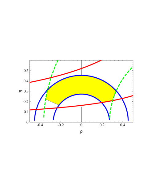
FIG. 4.: The allowed $\eta$ and $\rho$ ranges for $\hat{B}_{K}=1.0\pm 0.3$.

The gray region within the intersection of the curves is the range actually allowed after the correlation in $V_{cb}$ between eq. (129) and eq. (132) is taken into account. A further correlation is present in going from $\eta$ to Im $\lambda_{t}$ in eq. (128).

In the example of the VSA, where we have taken $\hat{B}_{K}=1.0\pm 0.3$, from Fig. 1 we obtain

$$0.51\times 10^{-4}\leq\mathop{\mbox{Im}}\lambda_{t}\leq 1.6\times 10^{-4}\;.$$ (138)

A further refinement of the analysis consists in assigning to each pair of $(\rho,\ \eta)$ values a Gaussian weight according to the deviations from the experimental central values of the computed parameters $V_{ub}/V_{cb}$, $\Delta M_{B_{d}}$, $\varepsilon$. In this way, a Gaussian distribution of the uncertainty on $\mathop{\mbox{Im}}\lambda_{t}$ (to be opposed to a flat one) is found and the error reduced. We will use for the discussion of the VSA the flat result of eq. (138).

In general the renormalization group invariant parameter $\hat{B}_{K}$ depends on the modeling of the hadronic matrix elements, so that different ranges of $\mathop{\mbox{Im}}\lambda_{t}$ should be expected according to the different approaches.

• In the München phenomenological approach, where $\hat{B}_{K}=0.75\pm 0.15$, a range

  $$0.86\times 10^{-4}\leq\mathop{\mbox{Im}}\lambda_{t}\leq 1.71\times 10^{-4}$$ (139)

  is found for a flat-distribution of the uncertainties in the input parameters, while the reduced range

  $$\mathop{\mbox{Im}}\lambda_{t}=(1.29\pm 0.22)\times 10^{-4}$$ (140)

  is obtained for a Gaussian treatment of the same uncertainties.

• In the Roma lattice calculation, which takes $\hat{B}_{K}=0.75\pm 0.15$, the range

  $$\cos\delta_{CP}=0.38\pm 0.23\ ,$$ (141)

  is obtained via the Gaussian treatment of the uncertainties, where $\delta_{CP}$ is the CKM phase. A result similar to eq. (140) is found by means of

  $$\mathop{\mbox{Im}}\lambda_{t}=|V_{cb}|^{2}\frac{|V_{ub}|}{|V_{cb}|}\sqrt{1-\cos^{2}\delta_{CP}}\;\,.$$ (142)

• In the Trieste $\chi$QM approach, which finds $\hat{B}_{K}=1.1\pm 0.2$, a flat scan of the input values leads to

  $$0.62\times 10^{-4}\leq\mathop{\mbox{Im}}\lambda_{t}\leq 1.4\times 10^{-4}\;.$$ (143)

  The larger value of $\hat{B}_{K}$ is responsible for the smaller values $\mathop{\mbox{Im}}\lambda_{t}$ obtained in this approach.

For a recent and detailed review on the determination of the CKM parameters see [Parodi:1998px].

VI Theoretical Predictions

We have now all the ingredients necessary to understand the various theoretical predictions for $\varepsilon^{\prime}/\varepsilon$ . Let us first rewrite eq. (15) in such a way that the relationship with the effective operators is more transparent.

The ratio $\varepsilon^{\prime}/\varepsilon$ can be written as

$$\frac{\varepsilon^{\prime}}{\varepsilon}=e^{i\phi}\ \frac{G_{F}\omega}{2\left|\epsilon\right|\mathop{\mbox{Re}}{A_{0}}}\>\mbox{Im}\,\lambda_{t}\>\>\left[\Pi_{0}-\frac{1}{\omega}\>\Pi_{2}\right]\;,$$ (144)

where, referring to the $\Delta S=1$ quark lagrangian of eq. (25),

$$\Pi_{0} = \frac{1}{\cos\delta_{0}}\sum_{i}y_{i}\,\mathop{\mbox{Re}}\langle Q_{i}\rangle_{0}\ (1-\Omega_{\eta+\eta^{\prime}})\;,$$ (145)

$$\Pi_{2} = \frac{1}{\cos\delta_{2}}\sum_{i}y_{i}\,\mathop{\mbox{Re}}\langle Q_{i}\rangle_{2}\;.$$ (146)

The phase of $\varepsilon^{\prime}/\varepsilon$ is [Maiani:1992ya]

$$\phi\,=\,\frac{\pi}{2}+\delta_{0}-\delta_{2}-\theta_{\epsilon}=(0\pm 4)^{0}\;,$$ (148)

and we can take it as vanishing. We assume everywhere that $CPT$ is conserved. An extra phase in addition to (148) would be present in the case of $CPT$ non-conservation: present experimental bounds constrain it to be at most of the order of $10^{-4}$ (for a review see [Maiani:1992ya]).

Notice the explicit presence of the final-state-interaction phases in eqs. (145) and (146). Their presence is a consequence of writing the absolute values of the amplitudes in term of their dispersive parts. Theoretically, given that in eq. (26) $\tau\ll 1$, we obtain

$$\tan\delta_{I}\simeq\frac{\sum_{i}z_{i}\,\mathop{\mbox{Im}}\langle Q_{i}\rangle_{I}}{\sum_{i}z_{i}\,\mathop{\mbox{Re}}\langle Q_{i}\rangle_{I}}\;.$$ (149)

A phenomenological estimate of the rescattering phases can be extracted from the elastic $\pi$-$\pi$ scattering. In chiral perturbation theory to $O(p^{4})$ one obtains [Gasser:1991ku]

$$\delta_{0}-\delta_{2}|_{s=m_{K}^{2}}=45^{0}\pm 6^{0}\;.$$ (150)

A more recent analysis of pion-nucleon collisions [Chell:1993wu], based on QCD sum rules and the extracted s-wave $\pi-\pi$ isospin scattering lengths, finds at the kaon mass scale

$$\delta_{0}=34.2^{0}\pm 2.2^{0}\;,\quad\quad\quad\delta_{2}=-6.9^{0}\pm 0.2^{0}\;,$$ (151)

and, accordingly,

$$\delta_{0}-\delta_{2}|_{s=m_{K}^{2}}=41^{0}\pm 4^{0}\;.$$ (152)

This result improves on older analyses [Basdevant:1974ru, Basdevant:1975aw, Froggatt:1977hu] for which

$$\delta_{0}=37^{0}\pm 3^{0}\;,\quad\quad\quad\delta_{2}=-7^{0}\pm 1^{0}\;.$$ (153)

All these results are consistent with each other and imply a misalignment of the $I=0$ over the $I=2$ amplitude by about 20% ($\cos\delta_{0}/\cos\delta_{2}\simeq 0.8$). Final state rescattering is not included in the VSA hadronic matrix elements, and in the lattice calculations, where the $K\to\pi$ transition is computed. Absorptive components appear when chiral loops are included, as in the $1/N_{c}$ approach of [Bardeen:1987uz] and in the $\chi$QM approach of the Trieste group. In the latter framework the direct determination of the rescattering phases gives at $O(p^{4})$ $\delta_{0}\simeq 20^{0}$ and $\delta_{2}\simeq-12^{0}$. Although these results show features which are in qualitative agreement with the phases extracted from pion-nucleon scattering, the deviation from the experimental data is sizeable, especially in the $I=0$ component. On the other hand, at $O(p^{4})$ the absorptive parts of the amplitudes are determined only at $O(p^{2})$ and disagreement with the measured phases should be expected. At any rate, the effect of such a discrepancy on eqs. (145)–(146) is numerically reduced by the $\cos\delta_{0,2}$ dependence. The authors have therefore chosen to input the experimental values of the rescattering phases in all parts of their analysis. This amounts to overstimating systematically the $I=0$ amplitude by about 15%. Since the analysis of the Trieste group is based on the fit of the $\Delta I=1/2$ rule with a 20% accuracy, such a bias is reabsorbed by the uncertainty found in the determination of $\left\langle\bar{q}q\right\rangle$.

Since Im $\lambda_{u}=0$ according to the standard conventions, the short-distance component of $\varepsilon^{\prime}/\varepsilon$ is determined by the Wilson coefficients $y_{i}$. Because, $y_{1}(\mu)=$ $y_{2}(\mu)=0$, the matrix elements of $Q_{1,2}$ do not directly enter the determination of $\varepsilon^{\prime}/\varepsilon$.

We can take, as fixed input values:

$$\frac{G_{F}\omega}{2\left|\epsilon\right|\mathop{\mbox{Re}}{A_{0}}}\simeq 349\ \mbox{GeV}^{-3}\;,\qquad\omega=1/22.2\;.$$ (154)

The large value in eq. (154) for $1/\omega$ comes from the $\Delta I=1/2$ selection rule.

The quantity $\Omega_{\eta+\eta^{\prime}}$, included in eq. (145) for notational convenience, represents the effect of the isospin-breaking mixing between $\pi^{0}$ and the etas, which generates a contribution to $A_{2}$ proportional to $A_{0}$. $\Omega_{\eta+\eta^{\prime}}$ can be written as [Donoghue:1986nm, Buras:1987wc]

$$\Omega_{\eta+\eta^{\prime}}=\frac{1}{3\sqrt{2}}\frac{1}{\omega}\left[\left(\cos\theta-\sqrt{2}\sin\theta\right)^{2}+\left(\sin\theta-\sqrt{2}\cos\theta\right)^{2}\frac{m_{\eta}^{2}-m_{\pi}^{2}}{m_{\eta^{\prime}}-m_{\pi}^{2}}\right]\frac{m_{d}-m_{u}}{m_{s}}\;,$$ (155)

where [Gasser:1985gg]

$$\frac{m_{d}-m_{u}}{m_{s}}=0.022\pm 0.002\;.$$ (156)

The mixing angle $\theta$ has been recently estimated in a model-independent way [Venugopal:1998fq] to be

$$\theta=-22^{0}\pm 3.3^{0}\;,$$ (157)

which is consistent with the values $\theta=-20^{0}\pm 4^{0}$ found in chiral perturbation theory [Donoghue:1986nm] and $\theta\simeq-22^{0}$ in the $1/N_{c}$ expansion [Gasser:1985gg].

The values above yield

$$\Omega_{\eta+\eta^{\prime}}=0.28\ ^{+0.03}_{-0.04}\;.$$ (158)

Smaller values are found once the uncertainty on the contribution of the $\eta^{\prime}$ is included [Cheng:1988dk]. For this reason, the more conservative range of values used in current estimates of $\varepsilon^{\prime}/\varepsilon$ is

$$\Omega_{\eta+\eta^{\prime}}=0.25\pm 0.10\ .$$ (159)

A Toy Models: VSA and VSA$+$

Before summarizing the current estimates of $\varepsilon^{\prime}/\varepsilon$ , it is useful to study some of the steps through which they are obtained in a toy model like that given by the VSA. As already pointed out, this model, because of its simplicity, can be considered as a convenient reference framework against which all other estimates are compared.

The VSA$+$ model that we introduced in Section IV is an attempt to improve on the VSA. It shows how a more refined treatment of the electroweak operators, which includes the $O(p^{2})$ corrections to the leading constant term, can lead to a larger value of $\varepsilon^{\prime}/\varepsilon$ .

The main purpose of these toy models is to illustrate in a simplified framework some general features of the calculation and the impact of some assumptions on the predicted value of $\varepsilon^{\prime}/\varepsilon$ . As we have discussed in Section IV, the VSA (as well as the VSA$+$) cannot give a reliable estimate because of the absence of a consistent scale and renormalization scheme matching with the NLO short-distance QCD calculation.

In the present discussion we use the Wilson coefficients in the HV scheme and set the reference value of the matching scale at 1 GeV (see table II). We will then gauge the renormalization scheme dependence of $\varepsilon^{\prime}/\varepsilon$ by varying the renormalization scheme from HV to NDR in the VSA amplitudes. Varying the matching scale around 1 GeV will show the systematic uncertainty related to the choice of the renormalization scale.

As we shall see, different groups work at different renormalization scales because of the peculiarities of their approaches. On the other hand, in a consistent approach the choice of the renormalization scale should be immaterial as long as observables are concerned. The same holds for the scheme dependence.

In addition to giving the $B_{i}$-parameters and the Wilson coefficients in a common scheme and at a common scale, one needs to specify the numerical value for the input parameter $\left\langle\bar{q}q\right\rangle$ which appear in the penguin matrix elements. We take the PCAC result, which at 1 GeV and for $m_{u}+m_{d}=12\pm 2.5$ MeV gives

$$\left\langle\bar{q}q\right\rangle=(-238\>^{+19}_{-14}\>\mbox{MeV})^{3}\,.$$ (160)

The mass $m_{s}$ is often used instead of $m_{d}$ and $m_{u}$. Such a change does not reduce the error and may even add further uncertainties due to the violations of PCAC that are larger in the $SU(3)$ case.

Each of the steps above, necessary in order to estimate $\varepsilon^{\prime}/\varepsilon$ , may carry in practice some model dependence and the reader must always bear in mind the assumptions that have entered in the final numerical values.

Let us now study how the various operators come together to give the final value of $\varepsilon^{\prime}/\varepsilon$ . Figure 5 shows the individual contribution of each operator in the VSA (gray histograms) and in the VSA$+$ (half-tone histograms). The dark histograms show how the various contributions are affected by changing the renormalization scheme from HV to NDR in the VSA$+$ case.

The VSA and VSA$+$ estimates only differ in the $Q_{7,8}$ matrix elements, as already discussed in section IV.A, while moving from HV to NDR affects mostly the $Q_{5,6}$ contributions (see Table II), thus leading to a potentially large effect on the VSA prediction for $\varepsilon^{\prime}/\varepsilon$ .

A central value of the order of $5\times 10^{-4}$ is found in the VSA, whereas in going from VSA to VSA$+$ the central value is increased by 50%. A 25% effect is then related to the renormalization scheme dependence in the VSA$+$, which corresponds to a 50% effect on the VSA.

Figure 5 shows clearly how systematic effects may sizeably move the $\varepsilon^{\prime}/\varepsilon$ value, due to the change in the destructive interference between gluonic and electroweak penguins.

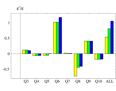
FIG. 5.: Anatomy of $\varepsilon^{\prime}/\varepsilon$ in the VSA in units of $10^{-3}$ at $\mu=1$ GeV with Im $\lambda_{t}=1.1\times 10^{-4}$. All other inputs are taken at their central values. Depicted in gray is the VSA, in half-tone the VSA$+$ and in black the effect of changing the renormalization scheme from HV to NDR.

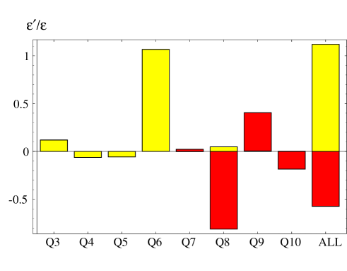
FIG. 6.: The distribution of the isospin $I=0$ (light gray) and $I=2$ (dark gray) contributions of each operator to $\varepsilon^{\prime}/\varepsilon$ (in units of $10^{-3}$) in the VSA.

Figure 6 shows, for the case of the VSA, the distribution of the $I=0$ and 2 components in the contributions of each operator. This figure is useful in disentangling the role and weight of the individual operators according to the isospin projections.

Finally, in Fig. 7 the value of $\varepsilon^{\prime}/\varepsilon$ in the VSA is shown as we continuously vary the two most relevant parameters: Im $\lambda_{t}$ and $\left\langle\bar{q}q\right\rangle$ . The two surfaces show in addition the dependence of $\varepsilon^{\prime}/\varepsilon$ on the short-distance input parameters $\Lambda_{\rm QCD}$ and $m_{t}$ as we vary them between their $1\sigma$ limits, and include also the dependence on the matching scale which is varied from 0.8 to 1.2 GeV. Fig. 7 is useful in showing the correlations between the input parameters and $\varepsilon^{\prime}/\varepsilon$ , which qualitatively hold beyond the specific model considered.

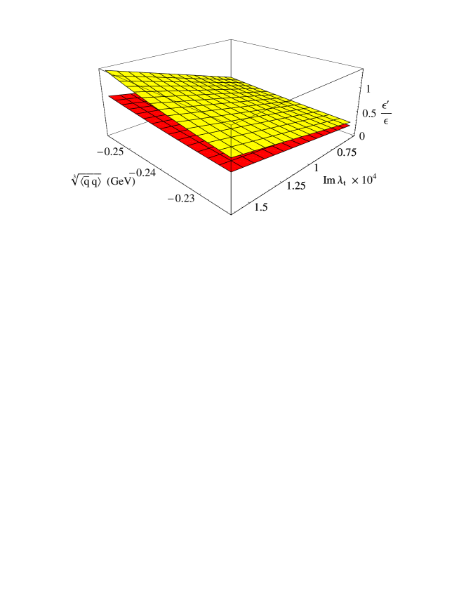
FIG. 7.: Parameter dependence of $\varepsilon^{\prime}/\varepsilon$ in the VSA, in units of $10^{-3}$. The upper (lighter) surface corresponds to taking $\mu=0.8$, $\Lambda_{\rm QCD}=380$ MeV and $m_{t}=161$ GeV, while the lower (darker) surface corresponds to $\mu=1.2$ GeV, $\Lambda_{\rm QCD}=300$ MeV and $m_{t}=173$ GeV.

From Fig. 7 we can finally extract the range of values taken by the parameter $\varepsilon^{\prime}/\varepsilon$ in the VSA, in the HV scheme, as we vary all relevant inputs. Taking into consideration the scale dependence of $\left\langle\bar{q}q\right\rangle$ we find

$$\varepsilon^{\prime}/\varepsilon=(0.5\>^{+0.6}_{-0.3})\,\times 10^{-3}\;.$$ (161)

Analogously, in the NDR scheme we obtain

$$\varepsilon^{\prime}/\varepsilon=(0.8\>^{+1.3}_{-0.5})\,\times 10^{-3}\;.$$ (162)

The large upper range of the NDR result is a consequence of the increase of the scheme dependence of the Wilson coefficients as $\Lambda_{\rm QCD}$ increases and the renormalization scale decreases.

While the toy models are useful in understanding how various possible contributions enter in the final estimate of $\varepsilon^{\prime}/\varepsilon$ , it is clear that some important factors are not included. Among them, the actual range of Im $\lambda_{t}$, strictly related to the determination of $\hat{B}_{K}$—which might be quite different from the naive VSA—and the consistency of the hadron matrix elements with the $\Delta I=1/2$ rule—which is important in assessing the confidence level of the $\varepsilon^{\prime}/\varepsilon$ predictions. For this reason, we now turn to estimates that incorporate these important features.

B Estimates of $\varepsilon^{\prime}/\varepsilon$

There are three groups for which an up-to-date calculation is available. In addition we will also briefly comment on some recent partial results obtained within the $1/N_{c}$ approach. We will identify the various groups by the names of the cities (München, Roma and Trieste) where most of the group members reside.

In table VII we collect some of the relevant inputs used by the three up-to-date estimates. There is overall agreement on the short-distance input parameters. The Trieste group differs from the other two in the value of $\hat{B}_{K}$, and therefore of Im $\lambda_{t}$, that is smaller, and for the inclusion of the FSI phases. The matching scales are different because of the peculiarities of each approach which lead to the quoted energy scales. The scale (and renormalization scheme) dependence of the final estimates is however rather small. We recall that while this stability is a formal property of the lattice and München phenomenological approaches, it is just a numerical feature of the Trieste estimate.

TABLE VII.: Comparison of input parameters in various approaches.

input	München	Roma	Trieste
$\Lambda_{\rm QCD}^{(4)}$	$325\pm 80$ MeV	$330\pm 100$ MeV	$340\pm 40$ MeV
$m_{t}(m_{t})$	$167\pm 6$ GeV	$167\pm 8$ GeV	$167\pm 6$ GeV
$m_{b}(m_{b})$	4.4 GeV	4.5 GeV	4.4 GeV
$m_{c}(m_{c})$	1.3 GeV	1.5 GeV	1.4 GeV
$\mu$	1.3 GeV	2 GeV	0.8 GeV
$m_{s}(\mu)$	$150\pm 20$ MeV	$128\pm 18$ MeV	$220\pm 20$ MeV
$\left\langle\bar{q}q\right\rangle(\mu)$	via PCAC from $m_{s}$	via PCAC from $m_{s}$	$(-240^{+30}_{-10}\ {\rm MeV})^{3}$
$\hat{B}_{K}$	$0.75\pm 0.15$	$0.75\pm 0.15$	$1.1\pm 0.2$
$\mathop{\mbox{Im}}\lambda_{t}\times 10^{4}$	$1.29\pm 0.22$	$1.29\pm 0.22$	$1.0\pm 0.4$
$\cos\delta_{0}$	1	1	0.8
$\cos\delta_{2}$	1	1	1
$\Omega_{\eta+\eta^{\prime}}$	$0.25\pm 0.05$	$0.25\pm 0.10$	$0.25\pm 0.10$

The experimental value of $m_{t}$ reported in Table VII—which has become available in the last few years—greatly helps in restricting the possible values of $\varepsilon^{\prime}/\varepsilon$ and, as we shall see, rules out, at least for a class of models, any mimicking of the superweak scenario by the standard model.

Starting with eq. (144), and given the input parameters in Table VII, the different estimates can be computed by writing $\varepsilon^{\prime}/\varepsilon$ in terms of the VSA to the matrix elements and the parameters $B_{i}$:

$$\sum_{i}y_{i}\left\langle Q_{i}\right\rangle_{0} = X\left(y_{4}B_{4}+\frac{1}{N_{c}}y_{3}B_{3}\right)-16\,\frac{\langle\bar{q}q\rangle^{2}L_{5}}{f^{6}}\,X\left(y_{6}B_{6}+\frac{1}{N_{c}}y_{5}B_{5}\right)$$ (165)

$$+\left(2\,\sqrt{3}\,\frac{\langle\bar{q}q\rangle^{2}}{f^{3}}+8\frac{\langle\bar{q}q\rangle^{2}L_{5}}{f^{6}}\,X\right)\left(y_{8}B_{8}+\frac{1}{N_{c}}y_{7}B_{7}\right)$$

$$+\frac{1}{2}X\left(y_{7}B_{7}+\frac{1}{N_{c}}y_{8}B_{8}\right)-\frac{1}{2}X\left[1-\frac{1}{N_{c}}\right]\left(y_{9}B_{9}-y_{10}B_{10}\right)\;,$$

and

$$\sum_{i}y_{i}\left\langle Q_{i}\right\rangle_{2} = \sqrt{6}\,\frac{\langle\bar{q}q\rangle^{2}}{f^{3}}\left(y_{8}B_{8}+\frac{1}{N_{c}}y_{7}B_{7}\right)-\frac{\sqrt{2}}{2}X\left(y_{7}B_{7}+\frac{1}{N_{c}}y_{8}B_{8}\right)$$ (167)

$$+\frac{\sqrt{2}}{2}X\left[1+\frac{1}{N_{c}}\right]\left(y_{9}B_{9}+y_{10}B_{10}\right)\;.$$

In eqs. (165)–(167) the values of the parameters $L_{5}$ and $\left\langle\bar{q}q\right\rangle$ are obtained according to eq. (95) and eq. (46) respectively, taking into account the scale dependence of the quark masses.

By inserting the appropriated $B_{i}$, taking into account their renormalization scheme dependence, the corresponding value of $\left\langle\bar{q}q\right\rangle$ (or $m_{s}$) and the other short-distance inputs, varied within the given uncertainties, the reader can recover the estimates for the various groups that are reported in the next few subsections.

1 Phenomenological Approach

In the phenomenological approach of the München group [Buras:1993dy, Buras:1996dq] the matching scale is chosen at $\mu=m_{c}$ because it is the scale at which penguins are decoupled from the $CP$ conserving amplitudes and some of the $B_{i}$ parameters can be extracted from the knowledge of the $\Delta I=1/2$ rule.

In this approach all $B_{i}$ except $B_{3,5,6}$ and $B_{8}^{(2)}$ are determined from the experimental values of physical processes. The operator $Q_{4}$ receives an enhancement due to the rather large value used for $B_{4}$ that comes from the fit of the $\Delta I=1/2$ rule with the assumption that $B_{3}=1$, as discussed in section IV.E.

The parameters $B_{6}$ and $B_{8}^{(2)}$ are varied within a 20% around the VSA values. The quark condensate is written in terms of $m_{s}$, which is then varied according to the uncertainty of its determination.

This procedure yields the two predictions [Buras:1996dq]

$$-1.2\times 10^{-4}\leq\varepsilon^{\prime}/\varepsilon\leq 16.0\times 10^{-4}\;,$$ (168)

for $m_{s}(m_{c})=150\pm 20$ MeV and

$$0\leq\varepsilon^{\prime}/\varepsilon\leq 43.0\times 10^{-4}\;,$$ (169)

for $m_{s}(m_{c})=100\pm 20$ MeV. This second range is included in order to study the implications of some recent lattice estimates of $m_{s}$ that found such a small values [Gupta:1997sa, Gough:1997kw]. Notice however that the lower range is somewhat extreme in the light of more recent lattice results now settling down at $m_{s}(\mbox{2 GeV})=110\pm 23$ MeV [Bhattacharya:1997ht] (which corresponds to $m_{s}(m_{c})=129\pm 27$ MeV). This range of $m_{s}$ values is also consistent with recent QCD sum rules estimates [Colangelo:1997uy, Jamin:1997sa]. On the other hand, a substantially larger determination of $m_{s}$ is obtained from the study of $\tau$ decays at LEP. A preliminary result from the ALEPH collaboration gives $m_{s}(m_{\tau})=172\pm 31$ MeV [Chen:1998mf]. It is therefore important for the determination of $\varepsilon^{\prime}/\varepsilon$ to understand better the value of this parameter, which via eq. (46) affects the size of the hadronic matrix elements of the most relevant operators.

For a Gaussian treatment of the uncertainties that affect the determination of $\mathop{\mbox{Im}}\lambda_{t}$, the values [Buras:1996dq]

$$\varepsilon^{\prime}/\varepsilon=(3.6\pm 3.4)\times 10^{-4}\;,$$ (170)

and

$$\varepsilon^{\prime}/\varepsilon=(10.4\pm 8.3)\times 10^{-4}\;,$$ (171)

are respectively found.

The same group also gives an approximated analytical formula, in terms of the penguin-box expansion, that is useful in discussing the impact in this estimate of the various input values:

$$\frac{\varepsilon^{\prime}}{\varepsilon}={\rm Im}\lambda_{t}\,F(x_{t})\,,$$ (172)

where

$$F(x_{t})=P_{0}+P_{X}\,X_{0}(x_{t})+P_{Y}\,Y_{0}(x_{t})+P_{Z}\,Z_{0}(x_{t})+P_{E}\,E_{0}(x_{t})\,.$$ (173)

The $x_{t}$-dependent functions in (173) are given, with an accuracy of better than 1%, by

$$X_{0}(x_{t})=0.660\,x_{t}^{0.575}\;, Y_{0}(x_{t})=0.315\,x_{t}^{0.78}\;,$$ (174)

$$Z_{0}(x_{t})=0.175\,x_{t}^{0.93}\;, E_{0}(x_{t})=0.564\,x_{t}^{-0.51}\;.$$ (175)

The coefficients $P_{i}$ are given in terms of $B_{6}^{(1/2)}\equiv B_{6}^{(1/2)}(m_{c})$, $B_{8}^{(3/2)}\equiv B_{8}^{(3/2)}(m_{c})$ and $m_{s}(m_{c})$ as follows

$$P_{i}=r_{i}^{(0)}+\left[\frac{158\>\mbox{MeV}}{m_{s}(m_{c})+m_{d}(m_{c})}\right]^{2}\left(r_{i}^{(6)}B_{6}^{(1/2)}+r_{i}^{(8)}B_{8}^{(3/2)}\right)\,.$$ (176)

The $P_{i}$ must be renormalization scale and scheme independent. They depend however on $\Lambda_{\rm QCD}$. Table VIII, taken from [Buras:1997fb], gives the numerical values of $r_{i}^{(0)}$, $r_{i}^{(6)}$ and $r_{i}^{(8)}$ for different values of $\Lambda_{\rm QCD}^{(4)}$ at $\mu=m_{c}$.

TABLE VIII.: The penguin-box expansion coefficients for various $\Lambda_{\rm QCD}^{(4)}$ as given by [Buras:1997fb]. Only the coefficients $r_{0}$ depend at the NLO on the renormalization scheme; the first raw gives their NDR values while the last row shows the corresponding values in the HV scheme. The results are given for $m_{s}(m_{c})=150$ MeV.

	$\Lambda_{\rm QCD}^{(4)}=245$ MeV			$\Lambda_{\rm QCD}^{(4)}=325$ MeV			$\Lambda_{\rm QCD}^{(4)}=405$ MeV
$i$	$r_{i}^{(0)}$	$r_{i}^{(6)}$	$r_{i}^{(8)}$	$r_{i}^{(0)}$	$r_{i}^{(6)}$	$r_{i}^{(8)}$	$r_{i}^{(0)}$	$r_{i}^{(6)}$	$r_{i}^{(8)}$
0	–2.674	6.537	1.111	–2.747	8.043	0.933	–2.814	9.929	0.710
$X$	0.541	0.011	0	0.517	0.015	0	0.498	0.019	0
$Y$	0.408	0.049	0	0.383	0.058	0	0.361	0.068	0
$Z$	0.178	–0.009	–6.468	0.244	–0.011	–7.402	0.320	–0.013	–8.525
$E$	0.197	–0.790	0.278	0.176	–0.917	0.335	0.154	–1.063	0.402
0	–2.658	5.818	0.839	–2.729	6.998	0.639	–2.795	8.415	0.398

It is important to stress that the approximated formula (173), with the numerical coefficient given in Table VIII, relies on the values of all $B_{i}$ used in the phenomenological approach, and great attention must be paid to the possible effects of the different patterns of $B_{i}$ and the scale at which they are computed when applying the same formula to other frameworks to compare predictions of $\varepsilon^{\prime}/\varepsilon$ in the standard model.

2 Lattice Approach

In the lattice approach of the Roma group [Ciuchini:1993tj, Ciuchini:1995cd, Ciuchini:1997kd], the matching scale is taken at $\mu=2$ GeV.

As it was for the München group, the operator $Q_{4}$ receives an enhancement due to the rather large value used for $B_{4}$ in order to fit the $\Delta I=1/2$ rule with the assumption $B_{3}=1$. The quark condensate is written in terms of $m_{s}$, which is then varied according to the uncertainty of its determination.

The parameters $B_{6}$ and $B_{8}^{(2)}$ are explicitly computed on the lattice, although the determination of $\left\langle Q_{6}\right\rangle$ suffers from large uncertainties (see section IV.D).

Only the result obtained via the Gaussian treatment of the errors in the input parameters is reported and yields [Ciuchini:1997kd]

$$\varepsilon^{\prime}/\varepsilon=(4.6\pm 3.0\pm 0.4)\times 10^{-4}\,,$$ (177)

where the first error is the variance of the distribution and the second one comes from the residual $\gamma_{5}$-scheme dependence. Fig. 8 from [Ciuchini:1997kd] shows the anatomy of $\varepsilon^{\prime}/\varepsilon$ in the lattice case. In this figure, the various contributions are shown in a manner similar to Fig. 5, with the additional separation of the electroweak components in isospin 0 and 2 amplitudes (as in Fig. 6 for the VSA).

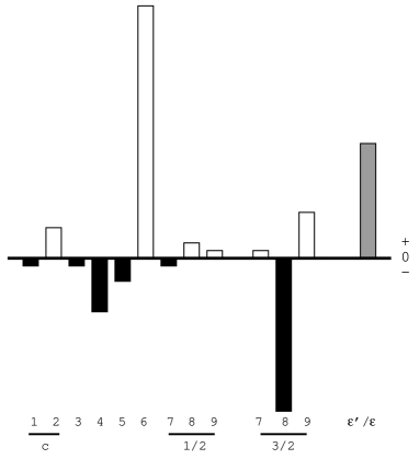
FIG. 8.: Anatomy of $\varepsilon^{\prime}/\varepsilon$ in the lattice approach in terms of the $I=0$ ($\Delta I=1/2$) and $I=2$ ($\Delta I=3/2$) components.

More recent estimates of $\hat{B}_{K}$ on the lattice [Kilcup:1997ye, Gupta:1997yt, Conti:1997qk], find a value larger than that used in deriving eq. (177), which makes Im $\lambda_{t}$ and, proportionally, $\varepsilon^{\prime}/\varepsilon$ even smaller.

3 Chiral Quark Model

In the $\chi$QM approach of the Trieste group [Bertolini:1996tp, Bertolini:1997nf], a rather low scale $\mu=0.8$ GeV is chosen because of the chiral-loop contribution that become perturbatively too large at scales higher than $\Lambda_{\chi}\approx m_{\rho}$, the chiral-symmetry breaking scale. Such a low energy scale for the matching makes some of the Wilson coefficients larger than in the other approaches and, correspondingly, more sensitive to higher order corrections.

Let us also recall that the scale and renormalization scheme stability of the computed observable is only a (welcomed) numerical feature and no attempt to address formally the cancellation of unphysical dependences is given. On the other hand, this estimate is the only one in which all $B_{i}$ are computed within the same model and in terms of a few basic parameters. It is also the only one for which the full $O(p^{4})$ amplitudes have been evaluated. It may therefore be quite useful in complementing the other estimates by illustrating characteristic patterns of the long-distance contributions.

The value of Im $\lambda_{t}$ is smaller than in the previous two estimates because of the rather large value for $\hat{B}_{K}$ (see Table III) that is found in this model.

The quark condensate is a primitive input parameter that is varied according to its determination in fitting the $\Delta I=1/2$ rule. The value in eq. (126) determined at the scale $\mu=0.8$ GeV by the Trieste group corresponds, via PCAC, to $m_{s}\simeq 220$ MeV. The quark masses appear explicitly in the $\chi$QM calculation at the NLO in momentum expansion and are treated as independent parameters. It is interesting to observe that in the $\chi$QM, because of the linear dependence on $\left\langle\bar{q}q\right\rangle$ of the $Q_{6}$ matrix element, contrasted to the quadratic dependence of $\langle Q_{8}\rangle$, decreasing the value of the quark condensate depletes the destructive interference between the two, and viceversa, partially compensating for the overall change of scale.

Taking into account a 1-$\sigma$ flat distribution of the input parameters the value [Bertolini:1997nf]

$$\varepsilon^{\prime}/\varepsilon=(1.7\>^{+1.4}_{-1.0})\times 10^{-3}$$ (178)

is found.

Figure 9 shows explicitly the contributions of the various operators, charted this time operator by operator as in Fig 5.

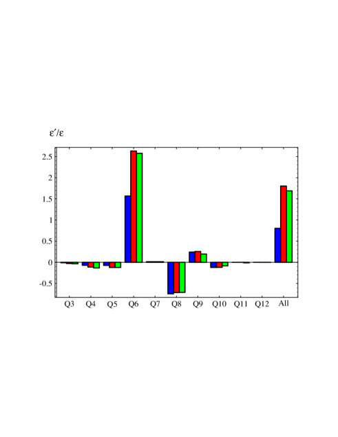
FIG. 9.: Anatomy of $\varepsilon^{\prime}/\varepsilon$ (in units of $10^{-3}$) within the $\chi$QM approach. In black the LO results (which includes the non-factorizable gluonic corrections), in half-tone the effect of the inclusion of chiral-loop corrections and in light gray the complete $O(p^{4})$ estimate.

A previous estimate of $\varepsilon^{\prime}/\varepsilon$ by the same group [Bertolini:1996tp] quoted the smaller value

$$\varepsilon^{\prime}/\varepsilon=(4\pm 5)\times 10^{-4}\;.$$ (179)

The change from (179) to (178) is due to the following improvements:

• Inclusion of the complete chiral lagrangian to $O(p^{2})$ as discussed in section III.A;

• Extension of the matrix element calculation to the $O(p^{4})$;

• Update of the short-distance analysis;

• New ranges of input parameters as determined by the updated fit of the $\Delta I=1/2$ rule [Bertolini:1997ir].

4 $1/N_{c}$ Approach

The approach based on a $1/N_{c}$ estimate of the hadron matrix elements, including chiral loops, has been first pursued by the München group [Bardeen:1987uz, Buchalla:1990we]. Eventually, it was dropped in favor of a phenomenological one that was judged to be better.

Successively, it was taken up by the Dortmund group [Paschos:1991as, Heinrich:1992en, Paschos:1996]. Unfortunately, many details of their work are not available and there is no complete and updated calculation. For this reason we did not include it in Table VII.

The latest available estimate quotes the value [Paschos:1996]

$$\varepsilon^{\prime}/\varepsilon=(9.9\pm 4.1)\times 10^{-4}\,,$$ (180)

for $m_{s}(1\ {\rm GeV})=175$ MeV. This value is the result of a $B_{6}$ larger than 1 and a $B_{8}^{(2)}$ smaller than 1 as obtained by including chiral-loop corrections in the matrix elements.

A very recent and new calculation of $B_{6}$ and $B_{8}$, which addresses systematically the problem of a consistent renormalization scale matching between chiral loops and Wilson coefficients, yields a smaller value for $B_{6}$ while a much suppressed value for $B_{8}^{(2)}$ is found [Hambye:1998sm]. No new estimate of $\varepsilon^{\prime}/\varepsilon$ has appeared yet. However, some of the relevant observables, as $B_{K}$ and the $I=0,2$ amplitudes, show at the present status of the calculation a quite poor scale stability [Hambye:1997dh, Kohler:1997pg], which may frustrate any attempt to produce a reliable estimate of $\varepsilon^{\prime}/\varepsilon$ .

C $\varepsilon^{\prime}/\varepsilon$ in the Standard Model: Summary and Outlook

If we consider that energy scales as different as $m_{t}$ and $m_{\pi}$ enter in an essential manner in the determination of the ratio $\varepsilon^{\prime}/\varepsilon$ , it is remarkable that this parameter can be predicted at all. Even more remarkable is the fact that all theoretical estimates are more or less consistent and a well-defined window of possible values emerges.

Figure 10 collects the estimates we have discussed and compares them with the two present (1998) experimental ranges from CERN (NA31) and FNAL (E731). We have also shown as a reference the results obtained in the simple VSA, in the HV and NDR schemes, as discussed at the beginning of this Section. We recall that the VSA error bars include a variation of the matching scale from 0.8 to 1.2 GeV.

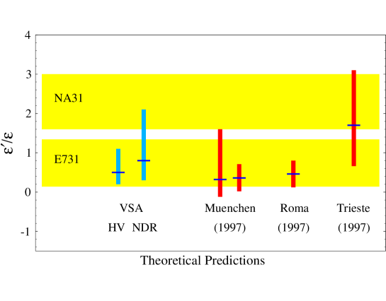
FIG. 10.: Current theoretical predictions for $\varepsilon^{\prime}/\varepsilon$ in units of $10^{-3}$ in the standard model. The horizontal short bars mark the central values of each prediction. The two gray areas correspond to the current NA31 and E731 1-$\sigma$ experimental bounds. In dark gray the naive VSA results are shown for comparison (the error bar includes a variation of the matching scale from 0.8 to 1.2 GeV).

The two error bars depicted for the München estimates correspond, from left to right, to flat and Gaussian scanning of the input data respectively. Also the reduced size of the error bar of the lattice result is due to the Gaussian treatment of the data.

The entire range between zero and, roughly $3\times 10^{-3}$ is spanned by the available standard model predictions, thus dispelling the belief (that has been around in the last few years) that values of the order of $10^{-3}$ were difficult to account for within the standard model.

Given the present theoretical and experimental results it is difficult to draw definite conclusions from their comparison beyond the fact that there are no inconsistencies. On the other hand the forthcoming experimental data may crucially help theorists in better understanding the role of non-perturbative QCD in the present estimates.

To have a pictorial impression of the dramatic improvement expected from the currently running experiments one must shrink the experimental ranges within a $\pm\>2\times 10^{-4}$ error band corresponding to two ticks on the vertical scale of Fig. 10. This is shown in Fig. 11 by the horizontal gray band drawn on the central value of the $2\sigma$ average of the NA31 and E731 results

$$\varepsilon^{\prime}/\varepsilon=(1.4\ \pm 1.6)\times 10^{-3}\ ,$$ (181)

which is obtained by following the PDG procedure for error inflation when central values are in disagreement [Winstein:1993sx].

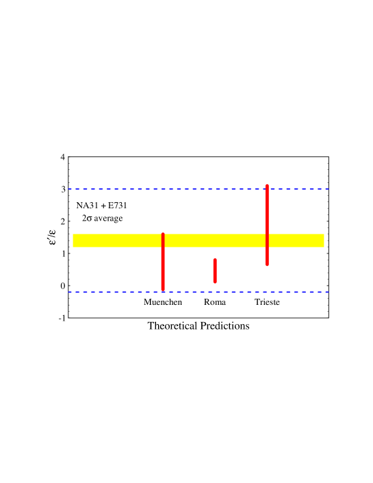
FIG. 11.: The combined NA31 and E731 experimental bounds (area within the dashed lines), are compared with the most updated theoretical estimates for $\varepsilon^{\prime}/\varepsilon$ (in units of $10^{-3}$). The gray horizontal band represents the future experimental sensitivity shown around the present experimental average value in eq. (181).

Such an improvement in the experimental results will certainly spur a new wave of theoretical analyses. We foresee at least three directions along which such a re-analysis may take place:

• Should the experimental results converge to a common error range of the order of few $10^{-4}$, it will be useful to focus the attention on the central values obtained by the various theoretical approaches in order to better understand the most relevant effects at work. As an example, consider the case that the new experimental central value turns out to be near or larger than the present average result. The comparison between the VSA and the VSA$+$ toy estimates discussed in the present review, together with the results of the Trieste group, suggest that the cancellation between the gluon and electroweak penguin operators may be substantially reduced once $(i)$ the complete set of the electroweak $O(p^{2})$ terms, and $(ii)$ higher order chiral corrections are taken into account. These effects can in part be included both in the München estimate, for those matrix elements that are not determined phenomenologically, and in the lattice prediction. Such effects may in fact account for larger central values than those presently obtained in those estimates.

• For what concerns the reduction of the theoretical error, in all estimates a crucial role is played by the knowledge of the relevant CKM entries. A large fraction of the theoretical error on $\varepsilon^{\prime}/\varepsilon$ is related to the uncertainty on $\mathop{\mbox{Im}}\lambda_{t}$, which amounts by inspection of eqs. (139)–(142), to a 30%$-$40% effect on the total error. The uncertainty on $\mathop{\mbox{Im}}\lambda_{t}$ is presently dominated by the determination of $\hat{B}_{K}$. In this respect, a precise determination of $\mathop{\mbox{Im}}\lambda_{t}$ from $B$-physics alone—as expected from the upcoming $B$-factories and hadronic facilities—will free this part of the analysis from large hadronic uncertainties and thus reduce the impact of non-perturbative QCD in the theoretical determination of $\varepsilon^{\prime}/\varepsilon$ .

• Progress in the lattice estimate of hadronic elements is to be expected in the next few years [Gupta:1998bm, Sharpe:1998hh]. A reliable estimate of the parameter $B_{6}$ is particularly needed. In addition, achieving the needed precision of the order of 10% or below in all relevant matrix elements implies going beyond the quenching approximation. The inclusion of higher-order chiral corrections can be also important. Much work is beeing done at present which indicates the possibility of addressing quantitatively this issue in the near future. It is from lattice QCD that we should expect a conclusive word on the matter.

VII New Physics and $\varepsilon^{\prime}/\varepsilon$

Physics beyond the standard model may enter the determination of $\varepsilon^{\prime}/\varepsilon$ in many ways. In particular, since the origin $CP$ violation is still unclear,

• It remains an open issue whether the $CP$ violation observed in the $\bar{K}^{0}$-$K^{0}$ system stems from complex Yukawa couplings or from a superweak interaction which goes beyond the standard model;

• Even maintaining that the observed $CP$ violation is not superweak in nature, other sources of $CP$ violations may be present in addition to, or replace the standard CKM phase in extensions of the standard model.

• Even if we insist that the CKM phase is the only source of $CP$ violation, new particle contributions to the Wilson coefficients of the effective quark Lagrangians still may be relevant for the detailed prediction of $CP$ violating observables.

However, given the discussion of the previous sections and considering in particular the comparison between the present theoretical and experimental results shown in Fig. 10, it appears to be a difficult task to disentangle new physics effects in $\varepsilon^{\prime}/\varepsilon$ .

Yet, one question that may be asked is whether the present experimental window allows for visible signals of non-standard physics. In order to answer this question we may take the average $2\sigma$ result of the NA31 and E731 experiments shown in Fig. 11 and compare it with the range obtained by the union of the most recent theoretical estimates (which is a reasonable, albeit biased, procedure).

It is clear that the case for observable signals of new physics is marginal, to say the least, and that, in order for new effects to become visible in $\varepsilon^{\prime}/\varepsilon$ , the next run of experimental data must converge to the most unlikely areas of the present range, thus pointing to values of $\varepsilon^{\prime}/\varepsilon$ larger than a few times $10^{-3}$, thereby confirming the 2$\sigma$ upper range of the NA31 result, or negative values, thus moving in the lower side of the 2$\sigma$ E731 range.

For this reason, we think that it is not necessary to present an exhaustive (and exhausting) review of all attempts to non-standard physics effects in $\varepsilon^{\prime}/\varepsilon$ . The interested reader may consult [Grimus:1988kn, Winstein:1993sx, Nir:1997nj, Fleischer:1997km] for reviews of possible new-physics effects in $CP$ violation.

It is nonetheless interesting to analyze whether specific models affect the standard model prediction via definite patterns. In order to do so, let us try to infer, inasmuch as possible in a model independent way, how new physics may affect the standard model prediction.

A Model Independent Analysis

The key ingredients for a theoretical prediction of $\varepsilon^{\prime}/\varepsilon$ are the determination of $\mathop{\mbox{Im}}\lambda_{t}$, from the experimental value of $\varepsilon$ and $B$-physics, and the calculation of all direct contributions to $\varepsilon^{\prime}$. These depend, on the short-distance side, from the values of the various components of the Wilson coefficients and, on the long-distance side, on the value of $\hat{B}_{K}$ and the $\Delta S=1$ matrix elements for $K\to\pi\pi$.

If we consider that the new effects modify only the short-distance aspects of the analysis, then the study of $\varepsilon$ exhibits a general feature: the new range of values for $\mathop{\mbox{Im}}\lambda_{t}$ obtained is always bounded from above by the maximum value given in Fig. 4 at $\rho=0$ by the $V_{ub}/V_{cb}$ measurement, which is a tree level bound and therefore robust to new effects.

As a consequence

• no sizeable enhancement of $\varepsilon^{\prime}/\varepsilon$ with respect to the standard model estimate can be expected from a modification of the short-distance part of $\varepsilon$.

On the other hand, the range of allowed values for $\mathop{\mbox{Im}}\lambda_{t}$ may be substantially reduced by new physics contributions, thus improving on the precision of the $\varepsilon^{\prime}/\varepsilon$ prediction.

Acting on the matchings of the $\Delta S=1$ Wilson coefficients $C_{i}$ in eq. (25) at $\mu=m_{W}$ affects the final outcome on $\varepsilon^{\prime}/\varepsilon$ . There are patterns on how changing the $C_{i}(m_{W})$ may affect the $y_{i}$ at the low energy scale ($\mu\simeq 1$ GeV) via strong and electromagnetic renormalizations.

In Table I, we have schematically reported the distribution of the different types of diagrams that determine the initial matching of the Wilson coefficients. Since new heavy particles may show their presence through their virtual exchange in the diagrams depicted in Fig. 1, and different type of diagrams show different short distance properties, it is important to keep an eye on how the relevant Wilson coefficients are generated

In Fig. 12 we show examples of how the various coefficients may mix via QCD renormalization and transmit the properties of the initial matchings to the other Wilson coefficients at the scale of the low energy process.

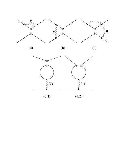
FIG. 12.: Effective diagrams showing the one-loop operator mixing via strong renormalization.

A direct look at the structure of the LO anomalous dimension matrix of the standard $\Delta S=1$ effective quark operators is sufficient to show qualitatively how the initial matching conditions may feed down to the final values of the various coefficients.

Here, as a quantitative and model independent test, we have varied the NLO (one-loop) standard-model initial matchings $Y_{i}\equiv C_{i}(m_{W})$ by factors of ($-1,0,2$) and observed the effects on the corresponding Wilson coefficients $y_{i}$ at the scale of 1 GeV. Our conclusions are the following:

• Only the varying of $Y_{2}$, $Y_{6}$, $Y_{7}$ and $Y_{9}$ leads to effects on the low energy $y_{i}$ larger than a few percents. ($Y_{8}$ and $Y_{10}$ matchings remain zero at the one-loop level).

• Changing the tree level Wilson coefficient $Y_{2}$, has a proportional effect on all the gluonic penguin coefficients ($y_{3,4,5,6}$) and similarly on $y_{11,12}$, because of the large additive renormalization induced via the insertion of $Q_{2}$ in the penguin like diagrams (d) in Fig. 12. The influence on $y_{6}$ of changing $Y_{2}$ by a few ten percents is therefore dramatic for the prediction of $\varepsilon^{\prime}/\varepsilon$ . On the other hand, one needs a new particle replacing tree level $W$ exchanges and tree level physics constrains dramatically these contributions. It is therefore unlikely to expect sizeable deviations of $Y_{2}$ from its standard model value.

• Changing $Y_{6}$ itself in the range given has no much effect on $y_{6}$ which is affected always less than 10%, and it affects $y_{8}$ at the percent level. Multiplicative renormalization is not the leading renormalization effect for the gluonic penguins.

• Changing $Y_{7}$ modifies proportionally $y_{7}$ and $y_{8}$ and may have therefore a dramatic impact on $\varepsilon^{\prime}/\varepsilon$ .

• Changing $Y_{9}$ modifies proportionally $y_{9}$ and $y_{10}$ and may affects $\varepsilon^{\prime}/\varepsilon$ at the few 10% level via the contribution of $Q_{9}$.

It seems therefore that the most relevant potential for new physics effects on $\varepsilon^{\prime}/\varepsilon$ resides in the electroweak penguin sector (see Table I). As a matter of fact [Buras:1998ed] have recently shown that bounding the contribution of the effective $\bar{s}dZ$ vertex via $\varepsilon^{\prime}/\varepsilon$ leads to the strongest constraints on some rare kaon decays which are governed by $Z-$penguin diagrams.

On the other hand, new physics modifications of the standard-model penguin and box diagrams for $\Delta S=1,2$ transitions affect also the corresponding $\Delta B=1,2$ amplitudes. It is therefore likely that in a specific model the experimental bounds coming from $B$ physics may indirectly constrain the deviations on the electroweak initial matchings within a few 10% [Nir:1997nj, Fleischer:1997km]. These bounds would make it hard for new physics to show up in visible deviations from the standard $\varepsilon^{\prime}/\varepsilon$ prediction.

The past literature on the subject confirms the general conclusion that we reached in the above discussion. The effect on $\varepsilon^{\prime}/\varepsilon$ of charged Higgs particles in the two Higgs model has been studied [Buchalla:1991fu]. The same problem has also been discussed in the more general framework of softly broken supersymmetry [Gabrielli:1995ff]. In both cases no significant departures from the standard model are expected once all bounds are properly implemented.

VIII Conclusions (March 1999)

On February 24, 1999 the KTeV collaboration has announced  a preliminary result based on the analysis of 20% of the data collected which gives

$$\mathop{\mbox{Re}}\>\varepsilon^{\prime}/\varepsilon=(28\pm 3.0\ {\rm(stat)}\pm 2.6\ {\rm(syst)}\pm 1.0\ {\rm(MC\ stat)})\times 10^{-4}\,.$$ (182)

This result largely deviates from the previous E731 value of eq. (24) and sits in the ballpark of the NA31 result (23). This value of $\varepsilon^{\prime}/\varepsilon$ , if confirmed, signals with high confidence the presence of direct CP violation in kaon decays, closing successfully a longstanding and challenging experimental quest. Theoretically, the superweak scenario [Wolfenstein:1964ks] is then excluded as the sole source of $CP$ violation.

Averaging (182) with (23) and (24), together with the older E731 result $\mathop{\mbox{Re}}\>\varepsilon^{\prime}/\varepsilon=(32\pm 30)\times 10^{-4}$, leads to the value

$$\mathop{\mbox{Re}}\>\varepsilon^{\prime}/\varepsilon=(21.8\pm 3.0)\times 10^{-4}\,.$$ (183)

In Fig. 13 we update the comparison between theory and experiment including the new KTeV result. The light gray area shows the $2\sigma$ range of the average in eq. (183).

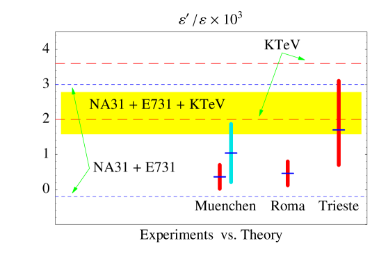
FIG. 13.: The new $2\sigma$ KTeV result (area enclosed by the long-dashed lines) is compared with the combined $2\sigma$ experimental bounds of NA31 and E731 (area enclosed by the short-dashed lines). The combined average in eq. (183) is shown ($2\sigma$) by the gray band. The München, Roma and Trieste theoretical estimates for $\varepsilon^{\prime}/\varepsilon$ are shown with their central values. The München and Roma predictions include gaussian treatment of the input parameters while the uncertainty in the Trieste estimate corresponds to flat parameter spanning. The second München prediction (light gray) corresponds to taking a low $m_{s}$ range (see eq. (171)).

The comparison between the present experimental average and the theoretical predictions shows a substantial deviation from the Roma and München estimates. Such a disagreement may be reduced by considering a light $m_{s}$ (see the discussion after eq. (168)). The two München predictions shown in Fig. 13 correspond to $m_{s}(m_{c})=150\pm 20$ and $m_{s}(m_{c})=100\pm 20$ (light gray), respectively.

The Trieste estimate is rather insensitive to $m_{s}$ since this parameter enters explicitely only at the NLO in the chiral expansion, while the value of the quark condensate is determined by the fit of the $\Delta I=1/2$ selection rule.

Let us recall that the most recent (quenched) lattice estimates of $m_{s}$ find $m_{s}(\mbox{2 GeV})=110\pm 23$ MeV [Bhattacharya:1997ht], corresponding to $m_{s}(m_{c})=129\pm 27$ MeV. This range of $m_{s}$ is also consistent with recent QCD sum rules estimates [Colangelo:1997uy, Jamin:1997sa], while a substantially larger determination of $m_{s}$ is obtained from $\tau$ decays at LEP. A preliminary result from the ALEPH collaboration gives $m_{s}(m_{\tau})=172\pm 31$ MeV [Chen:1998mf]. In order to assess the theoretical implications of the KTeV result it will be important to better understand the value of $m_{s}$, that is currently used to parametrizee the hadronic matrix elements of the crucial operators $Q_{6}$ and $Q_{8}$ (for a more detailed discussion see [Keum:1999gw]).

On the other hand, as we argue in the summary of section VI, it is premature to take a value of $\varepsilon^{\prime}/\varepsilon$ at the $10^{-3}$ level as a signal of new physics. In particular, it is worth observing that:

• One of the standard model predictions, which via the $\Delta I=1/2$ selection obtains all matrix elements, is in good agreement with the experimental average in eq. (183);

• As it is shown by the VSA and VSA+ toy models, and as it appears from the Trieste calculation, the inclusion of NLO order chiral corrections might alone conspire toward increasing the standard model value obtained in the present phenomenological and quenched lattice predictions.

At any rate, efforts on improving all theoretical estimates are now required. In particular, a confident assessement of the size of $B_{6}$ from lattice will be of crucial relevance.

As discussed in section VI.C, the uncertainty in all present theoretical estimates may be substantially reduced by a better determination of $\mathop{\mbox{Im}}\lambda_{t}$, whose error is presently dominated by the uncertainty on $\hat{B}_{K}$. A precise determination of $\mathop{\mbox{Im}}\lambda_{t}$ is expected in the upcoming years from $B$-physics at the $B$-factories and at the hadronic colliders. In addition, the rare kaon decays $K_{L}\to\pi^{0}\nu\bar{\nu}$ and $K^{+}\to\pi^{+}\nu\bar{\nu}$ provide together a clean probe of $\mathop{\mbox{Im}}\lambda_{t}$ [Buchalla:1996fp]. While the latter may be seen at the Brokhaven National Laboratory within the next year, a new experiment at the same laboratory has been approved to measure Br$(K_{L}\to\pi^{0}\nu\bar{\nu})$ with a 10% precision by the year 2005. This will allow a determination of $\mathop{\mbox{Im}}\lambda_{t}$ with a similar accuracy.

In conclusion, the determination of $\varepsilon^{\prime}/\varepsilon$ is a great challenge to both experimentalists and theorists. As more precise experimental data become available, improvements in the theoretical calculations are also expected. The interplay of the two will hopefully shed more light on the flavor structure of the standard model and on some non-perturbative aspects of QCD.

- [1]
- [2] [] Antonelli, V., S. Bertolini, J. O. Eeg, M. Fabbrichesi, and E. I. Lashin, 1996, Nucl. Phys. B469, 143–180.
- [3]
- [4] [] Banner, M., et al., 1972, Phys. Rev. Lett. 28, 1209.
- [5]
- [6] [] Bardeen, W. A., A. J. Buras, and J. M. Gerard, 1987, Nucl. Phys. B293, 787.
- [7]
- [8] [] Barnett, R. M., et al., 1996, Phys. Rev. D54, 1–720.
- [9]
- [10] [] Barr, G. D., et al., 1993, Phys. Lett. B317, 233–242.
- [11]
- [12] [] Basdevant, J. L., C. D. Froggatt, and J. L. Petersen, 1974, Nucl. Phys. B72, 413.
- [13]
- [14] [] Basdevant, J. L., P. Chapelle, C. Lopez, and M. Sigelle, 1975, Nucl. Phys. B98, 285.
- [15]
- [16] [] Bernstein, R. H., et al., 1985, Phys. Rev. Lett. 54, 1631.
- [17]
- [18] [] Bertolini, S., J. O. Eeg, and M. Fabbrichesi, 1995, Nucl. Phys. B449, 197–228.
- [19]
- [20] [] Bertolini, S., J. O. Eeg, and M. Fabbrichesi, 1996, Nucl. Phys. B476, 225–254.
- [21]
- [22] [] Bertolini, S., J. O. Eeg, M. Fabbrichesi, and E. I. Lashin, 1998a, Nucl. Phys. B514, 63–92.
- [23]
- [24] [] Bertolini, S., J. O. Eeg, M. Fabbrichesi, and E. I. Lashin, 1998b, Nucl. Phys. B514, 93–112.
- [25]
- [26] [] Bhattacharya, T., and R. Gupta, 1998, Nucl. Phys. Proc. Suppl. 63, 95.
- [27]
- [28] [] Bijnens, J., 1993, Int. J. Mod. Phys. A8, 3045.
- [29]
- [30] [] Bijnens, J., 1996, Phys. Rept. 265, 369–446.
- [31]
- [32] [] Bijnens, J., and J. Prades, 1995, Nucl. Phys. B444, 523–562.
- [33]
- [34] [] Bijnens, J., and M. B. Wise, 1984, Phys. Lett. 137B, 245.
- [35]
- [36] [] Bijnens, J., C. Bruno, and E. de Rafael, 1993, Nucl. Phys. B390, 501–541.
- [37]
- [38] [] Bijnens, J., E. Pallante, and J. Prades, 1998, Nucl. Phys. B521, 305.
- [39]
- [40] [] Black, J. K., et al., 1985, Phys. Rev. Lett. 54, 1628.
- [41]
- [42] [] Breitenlohner, P., and D. Maison, 1977, Commun. Math. Phys. 52, 55.
- [43]
- [44] [] Buchalla, G., A. J. Buras, and M. K. Harlander, 1990, Nucl. Phys. B337, 313–362.
- [45]
- [46] [] Buchalla, G., A. J. Buras, M. K. Harlander, M. E. Lautenbacher, and C. Salazar, 1991, Nucl. Phys. B355, 305–329.
- [47]
- [48] [] Buchalla, G., and A. J. Buras, 1996, Phys. Rev. D54, 6782–6789.
- [49]
- [50] [] Buras, A. J., and J. M. Gerard, 1987, Phys. Lett. 192B, 156.
- [51]
- [52] [] Buras, A. J., and L. Silvestrini, 1998, hep-ph/9811471.
- [53]
- [54] [] Buras, A. J., and R. Fleischer, 1997, hep-ph/9704376.
- [55]
- [56] [] Buras, A. J., M. Jamin, and M. E. Lautenbacher, 1993a, Nucl. Phys. B400, 75–102.
- [57]
- [58] [] Buras, A. J., M. Jamin, and M. E. Lautenbacher, 1996, Phys. Lett. B389, 749–756.
- [59]
- [60] [] Buras, A. J., M. Jamin, and P. H. Weisz, 1990, Nucl. Phys. B347, 491–536.
- [61]
- [62] [] Buras, A. J., M. Jamin, E. Lautenbacher, and P. H. Weisz, 1992, Nucl. Phys. B370, 69–104.
- [63]
- [64] [] Buras, A. J., M. Jamin, M. E. Lautenbacher, and P. H. Weisz, 1993, Nucl. Phys. B400, 37–74.
- [65]
- [66] [] Buras, A., M. Jamin, and M. E. Lautenbacher, 1993b, Nucl. Phys. B408, 209–285.
- [67]
- [68] [] Chau, L.-L., 1983, Phys. Rept. 95, 1.
- [69]
- [70] [] Chell, E., and M. G. Olsson, 1993, Phys. Rev. D48, 4076–4081.
- [71]
- [72] [] Chen, S., 1998, Nucl. Phys. Proc. Suppl. 64, 265.
- [73]
- [74] [] Cheng, H.-Y., 1988, Phys. Lett. 201B, 155.
- [75]
- [76] [] Chivukula, R. S., J. M. Flynn, and H. Georgi, 1986, Phys. Lett. 171B, 453.
- [77]
- [78] [] Christenson, J. H., J. W. Cronin, V. L. Fitch, and R. Turlay, 1964, Phys. Rev. Lett. 13, 138.
- [79]
- [80] [] Christenson, J. H., et al., 1979a, Phys. Rev. Lett. 43, 1212.
- [81]
- [82] [] Christenson, J. H., et al., 1979b, Phys. Rev. Lett. 43, 1209.
- [83]
- [84] [] Ciuchini, M., 1997, Nucl. Phys. Proc. Suppl. 59, 149.
- [85]
- [86] [] Ciuchini, M., E. Franco, G. Martinelli, and L. Reina, 1993, Phys. Lett. B301, 263–271.
- [87]
- [88] [] Ciuchini, M., E. Franco, G. Martinelli, and L. Reina, 1994, Nucl. Phys. B415, 403–462.
- [89]
- [90] [] Ciuchini, M., E. Franco, G. Martinelli, L. Reina, and L. Silvestrini, 1995, Z. Phys. C68, 239–256.
- [91]
- [92] [] Colangelo, P., F. D. Fazio, G. Nardulli, and N. Paver, 1997, Phys. Lett. B408, 340–346.
- [93]
- [94] [] Conti, L., et al., 1998, Phys. Lett. B421, 273–282.
- [95]
- [96] [] Cronin, J. A., 1967, Phys. Rev. 161, 1483–1494.
- [97]
- [98] [] de Rafael, E., 1994, CP Violation and the Limits of the Standard Model (Benjamin/Cummings, Menlo Park, California).
- [99]
- [100] [] Donoghue, J. F., 1984, Phys. Rev. D30, 1499.
- [101]
- [102] [] Donoghue, J. F., E. Golowich, B. R. Holstein, and J. Trampetic, 1986, Phys. Lett. 179B, 361.
- [103]
- [104] [] Dupont, Y., and T. N. Pham, 1984, Phys. Rev. D29, 1368.
- [105]
- [106] [] Ecker, G., J. Kambor, and D. Wyler, 1993, Nucl. Phys. B394, 101–138.
- [107]
- [108] [] Ellis, J., M. K. Gaillard, and D. V. Nanopoulos, 1976, Nucl. Phys. B109, 213.
- [109]
- [110] [] Ellis, J., M. K. Gaillard, D. V. Nanopoulos, and S. Rudaz, 1977, Nucl. Phys. B131, 285.
- [111]
- [112] [] Esposito-Farese, G., 1991, Z. Phys. C50, 255–274.
- [113]
- [114] [] Espriu, D., E. de Rafael, and J. Taron, 1990, Nucl. Phys. B345, 22–56.
- [115]
- [116] [] Fabbrichesi, M., and E. I. Lashin, 1996, Phys. Lett. B387, 609–613.
- [117]
- [118] [] Fleischer, R., 1997, hep-ph/9709291.
- [119]
- [120] [] Flynn, J. M., and L. Randall, 1989, Phys. Lett. B224, 221.
- [121]
- [122] [] Froggatt, C. D., and J. L. Petersen, 1977, Nucl. Phys. B129, 89.
- [123]
- [124] [] Gabrielli, E., and G. F. Giudice, 1995, Nucl. Phys. B433, 3–25.
- [125]
- [126] [] Gasser, J., and H. Leutwyler, 1984, Ann. Phys. 158, 142.
- [127]
- [128] [] Gasser, J., and H. Leutwyler, 1985, Nucl. Phys. B250, 465.
- [129]
- [130] [] Gasser, J., and U. G. Meissner, 1991, Phys. Lett. B258, 219–224.
- [131]
- [132] [] Gavela, M. B., A. L. Yaouanc, L. Oliver, O. Pene, and J. C. Raynal, 1984, Phys. Lett. 148B, 225.
- [133]
- [134] [] Gell-Mann, M., and A. Pais, 1954, Proc. Glasgow Conf. p. 342.
- [135]
- [136] [] Georgi, H., 1984, Weak Interactions and Modern Particle Theory (Benjamin/Cummings, Menlo Park, California).
- [137]
- [138] [] Gibbons, L. K., et al., 1997, Phys. Rev. D55, 6625–6715.
- [139]
- [140] [] Gilman, F. J., and M. B. Wise, 1979a, Phys. Rev. D20, 2392.
- [141]
- [142] [] Gilman, F. J., and M. B. Wise, 1979b, Phys. Lett. 83B, 83.
- [143]
- [144] [] Gough, B. J., et al., 1997, Phys. Rev. Lett. 79, 1622–1625.
- [145]
- [146] [] Grimus, W., 1988, Fortschr. Phys. 36, 201.
- [147]
- [148] [] Gupta, R., 1998, hep-ph/9801412.
- [149]
- [150] [] Gupta, R., and T. Bhattacharya, 1997, Phys. Rev. D55, 7203–7217.
- [151]
- [152] [] Gupta, R., T. Bhattacharya, and S. Sharpe, 1997, Phys. Rev. D55, 4036–4054.
- [153]
- [154] [] Hambye, T., 1997, Acta Phys. Pol. B28, 2479.
- [155]
- [156] [] Hambye, T., G. O. Kohler, E. A. Paschos, P. H. Soldan, and W. A. Bardeen, 1998, Phys. Rev. D58, 014017.
- [157]
- [158] [] Heinrich, J., E. A. Paschos, J. M. Schwarz, and Y. L. Wu, 1992, Phys. Lett. B279, 140–144.
- [159]
- [160] [] Herrlich, S., and U. Nierste, 1994, Nucl. Phys. B419, 292–322.
- [161]
- [162] [] Herrlich, S., and U. Nierste, 1995, Phys. Rev. D52, 6505–6518.
- [163]
- [164] [] Herrlich, S., and U. Nierste, 1996, Nucl. Phys. B476, 27–88.
- [165]
- [166] [] Holder, M., 1997, Proceedings of the Workshop on K Physics, Orsay, France, ed. L. Iconomidou-Fayard (Editions Frontieres, 1997).
- [167]
- [168] [] Holder, M., et al., 1972, Phys. Lett. B40, 141.
- [169]
- [170] [] Inami, T., and C. S. Lim, 1981, Prog. Theor. Phys. 65, 297.
- [171]
- [172] [] Jamin, M., 1998, Nucl. Phys. Proc. Suppl. 64, 250.
- [173]
- [174] [] Kambor, J., J. Missimer, and D. Wyler, 1990, Nucl. Phys. B346, 17–64.
- [175]
- [176] [] Kambor, J., J. Missimer, and D. Wyler, 1991, Phys. Lett. B261, 496–503.
- [177]
- [178] [] Keum, Y.-Y., U. Nierste, and A. I. Sanda, 1999, hep-ph/9903230.
- [179]
- [180] [] Kilcup, G., R. Gupta, and S. R. Sharpe, 1998, Phys. Rev. D57, 1654.
- [181]
- [182] [] Kobayashi, M., and T. Maskawa, 1973, Prog. Theor. Phys. 49, 652.
- [183]
- [184] [] Kohler, G. O., 1998, hep-ph/9806224.
- [185]
- [186] [] Landau, L., 1957, Nucl. Phys. 3, 127.
- [187]
- [188] [] Lusignoli, M., 1989, Nucl. Phys. B325, 33.
- [189]
- [190] [] Lusignoli, M., L. Maiani, G. Martinelli, and L. Reina, 1992, Nucl. Phys. B369, 139–170.
- [191]
- [192] [] Maiani, L., G. Pancheri, and N. Paver, 1992, The DAPHNE Physics Handbook. Vol. 1, 2, Frascati, Italy: INFN (1992) 611 p.
- [193]
- [194] [] Manohar, A., and H. Georgi, 1984, Nucl. Phys. B234, 189.
- [195]
- [196] [] Martinelli, G., 1998, hep-lat/9810013.
- [197]
- [198] [] Narison, S., 1995, Phys. Lett. B351, 369–374.
- [199]
- [200] [] Nir, Y., 1992, SLAC-PUB-5874.
- [201]
- [202] [] Nir, Y., 1997, hep-ph/9709301.
- [203]
- [204] [] O’Dell, V., 1997, Proceedings of the Workshop on K Physics, Orsay, France, ed. L. Iconomidou-Fayard (Editions Frontieres, 1997).
- [205]
- [206] [] Parodi, F., P. Roudeau, and A. Stocchi, 1998, hep-ph/9802289.
- [207]
- [208] [] Paschos, E. A., 1996, Proceedings of the 27th Lepton-Photon Symposium, Beijing (August 1995).
- [209]
- [210] [] Paschos, E. A., and Y. L. Wu, 1991, Mod. Phys. Lett. A6, 93–106.
- [211]
- [212] [] Patera, V., 1997, Proceedings of the Workshop on K Physics, Orsay, France, ed. L. Iconomidou-Fayard (Editions Frontieres, 1997).
- [213]
- [214] [] Pich, A., and E. de Rafael, 1991, Nucl. Phys. B358, 311–382.
- [215]
- [216] [] Sharpe, S., 1994, CP Violation and the Limits of the Standard Model (Benjamin/Cummings, Menlo Park, California).
- [217]
- [218] [] Sharpe, S. R., 1997, Nucl. Phys. Proc. Suppl. 53, 181–198.
- [219]
- [220] [] Sharpe, S. R., 1998.
- [221]
- [222] [] Shifman, M. A., A. I. Vainshtein, and V. I. Zakharov, 1977, Nucl. Phys. B120, 316.
- [223]
- [224] [] ’t Hooft, G., and M. Veltman, 1972, Nucl. Phys. B44, 189.
- [225]
- [226] [] Tipton, P. L., 1997, Proceedings of the 28th ICHEP (Warsaw), eds. Z. Ajduk and A. K. Wroblewsky, p. 123 (World Scientific, Singapore 1997).
- [227]
- [228] [] Vainshtein, A. I., V. I. Zakharov, and M. A. Shifman, 1975, JETP Lett. 22, 55–56.
- [229]
- [230] [] Vainshtein, A. I., V. I. Zakharov, and M. A. Shifman, 1977, Sov. Phys. JETP 45, 670.
- [231]
- [232] [] Venugopal, E. P., and B. R. Holstein, 1998, Phys. Rev. D57, 4397–4402.
- [233]
- [234] [] Watson, K. M., 1952, Phys. Rev. 88, 1163–1171.
- [235]
- [236] [] Weinberg, S., 1979, Physica 96A, 327.
- [237]
- [238] [] Weinberg, S., 1980, Phys. Lett. 91B, 51.
- [239]
- [240] [] Wilson, K. G., 1971, Phys. Rev. D3, 1818.
- [241]
- [242] [] Winstein, B., and L. Wolfenstein, 1993, Rev. Mod. Phys. 65, 1113–1148.
- [243]
- [244] [] Wolfenstein, L., 1964, Phys. Rev. Lett. 13, 562–564.
- [245]
- [246] [] Wu, C. S., E. Ambler, R. W. Hayward, D. D. Hoppes, and R. P. Hudson, 1957, Phys. Rev. 105, 1413.
- [247]