Finite-size effects on multibody neutrino exchange

Abstract

The effect of multibody massless neutrino exchanges between neutrons inside a finite-size neutron star is studied. We use an effective Lagrangian, which incorporates the effect of the neutrons on the neutrinos. Following Schwinger, it is shown that the total interaction energy density is computed by comparing the zero point energy of the neutrino sea with and without the star. It has already been shown that in an infinite-size star the total energy due to neutrino exchange vanishes exactly. The opposite claim that massless neutrino exchange would produce a huge energy is due to an improper summation of an infrared-divergent quantity. The same vanishing of the total energy has been proved exactly in the case of a finite star in a one-dimensional toy model. Here we study the three-dimensional case. We first consider the effect of a sharp star border, assumed to be a plane. We find that there is a non-vanishing of the zero point energy density difference between the inside and the outside due to the refraction index at the border and the consequent non-penetrating waves. An analytical and numerical calculation for the case of a spherical star with a sharp border confirms that the preceding border effect is the dominant one. The total result is shown to be infrared-safe, thus confirming that there is no need to assume a neutrino mass. The ultraviolet cut-offs, which correspond in some sense to the matching of the effective theory with the exact one, are discussed. Finally the energy due to long distance neutrino exchange is of the order of $10^{-8}$–$10^{-13}\ {\mathrm{GeV}\hbox{ per neutron}}$, i.e. negligible with respect to the neutron mass density.

CERN-TH/98-40

February 1998

I Introduction

The massless neutrino exchange interaction between neutrons, protons, etc., is a long-range force [1]–[3]. In a previous work [4], the long-range interaction effects on the stability of a neutron star due to multibody exchange of massless neutrinos have been studied. We have shown that the total effect of the many-body forces of this type results in an infrared well-behaved contribution to the energy density of the star and that it is negligible with respect to the star mass density. This is in agreement with two recent non-perturbative calculations done by Kachelriess [5] and by Kiers and Tytgat [6].

This work is in contradiction with the repeated claim by Fischbach [7] that, unless the neutrino is massive, neutrino exchange renders a neutron star unstable, as the induced self-energy exceeds the mass of the star because of the infrared effects associated to neutrino exchange between four or more neutrons. In our opinion, the latter “catastrophic” result is a consequence of summing up large infrared terms in perturbation outside the radius of convergence of the perturbative series. The non-perturbative use of an effective Lagrangian immediately gives the result without recourse to the perturbative series, and the result is small.

Smirnov and Vissani [8], following the same method as in ref. [7], summing up multibody exchange contributions order by order, showed that the 2-body contribution is damped by the blocking effect of the neutrino sea [9]. They guessed that this damping would apply to many-body contributions, and hence would reduce the catastrophic effect claimed by Fischbach. In our previous work [4], we also considered the effect of the neutrino sea inside the neutron star. This effect has been introduced in our non-perturbative calculation by using Feynman propagators of neutrinos inside a dense medium, which incorporate the condensate term. We noticed that this condensate is present, but in our opinion it is not the most important of the effects that neutralize the catastrophic effect expected by Fischbach, since it only brings a tiny change to the non-perturbatively summed interaction energy, leaving unchanged our conclusion that the weak self-energy is infrared-safe.

We have also stressed in [4] that the neutrino condensate was related to the existence of a border . This was demonstrated in the ($1\ +\ 1$)-dimensional star in [10]: the blocking effect, which implies the trapping of the neutrinos inside the star while the antineutrinos are repelled from it, is a natural consequence of the existence of a border. Indeed a proper treatment of the effect of the border automatically incorporates the condensate contribution as a consequence of the appropriate boundary conditions for the neutrino Feynman propagator inside the star.

Since our treatment directly incorporates the neutrino sea effect and, on the other hand, since we stick to our strategy of directly computing the total neutrino interaction energy by using an effective Lagrangian, we have in a sense thus generalized the result of Smirnov and Vissani [8] because our result holds in a non-perturbative way and accounts for all the $n$-body contributions, while theirs holds for $2$-body contributions only.

It has been objected [11] to our study [4] that we worked in an approximation where we neglected the border of the neutron star. Our belief is that this simplifying hypothesis does not change the fundamental result that the total effect of the multiple neutrino exchange to the energy density of the star is not infrared-divergent.

Indeed, in [10] we have proved that, in $(1\ +\ 1)$ dimensions with borders, the result of [4] for the infinite star without borders is kept unchanged: the net interaction energy due to long-range neutrino exchange is exactly zero. This result was obtained by computing Feynman vacuum loops with neutrino propagators derived from the effective Lagrangian, which incorporates the neutron interaction. The latter propagators are not translational-invariant, because of the star borders. We have found a physically simple explanation for the vanishing of the net interaction energy. It relies on the fact that the negative energy states, in the presence of the star and without the star, are in a one-to-one correspondence and have exactly the same energy density. It results that the zero point energy is the same with and without the star, for any density profile of the star.

The main goal of the present work is to follow on taking into account the finite-size and border effects. Two main conclusions of ref. [10] are useful for the ($3\ +\ 1$)-dimensional star: i) the natural connection between the neutrino sea and the border, ii) the correct definition of the zero-energy level of the Dirac sea.

From [10], we know that the zero-energy level of the Dirac sea has to be adjusted by comparing the asymptotic behaviour of the wave functions far outside the star with the free solutions in the absence of the star. From there, we know the correct $i\epsilon$ prescription, which has to be imposed in the propagators of the neutrinos in the presence of the star; we could in principle compute the closed loops to get the vacuum energy density. However, this approach is technically very difficult. A simpler method, the derivation of which is recalled in section II, is to simply add the energy density of the negative energy solutions in the presence of the star, minus the same in the absence of the star.

The vanishing of the neutrino exchange energy density in the star, found in the case of an infinite star [4] and in $(1\ +\ 1)$ dimensions [10], which will be summarized in section III, is not valid in $(3\ +\ 1)$ dimensions. The main reason for that will be illustrated in section IV by zooming to the border effect, i.e. considering a plane border in $(3\ +\ 1)$ dimensions. There is a non-trivial refraction index that modifies the wave energy densities as they penetrate the star. Some waves are forbidden to penetrate and this yelds the dominant contribution.

In section V, we perform analytical and numerical calculations, which take into account the curvature of the border and use a spherical star with a sharp border. We find a very simple approximate formula for the zero point neutrino energy density in the star, and demonstrate numerically the validity of this approximation. It results that indeed the neutrino-induced energy density in the star does not vanish and is dominantly explained by the above-mentioned border effect.

In any case, these non-vanishing neutrino exchange energy densities are all perfectly regular in the infrared and do not present any resemblance to Fischbach’s effect. On the other hand they are ultraviolet-singular. This is not unexpected since anyhow our effective Lagrangian is only valid below some energy scale where the neutrons may be considered at rest. In section VI, we also discuss in some detail the effect of decoherence for distances larger than the neutrino mean-free path, which smoothes down the ultraviolet singularity.

We conclude that the stability of compact and dense objects such as a white dwarfs, neutron stars, etc., are not affected by the neutrino exchange, even if neutrinos are massless.

II General Formalism

In our calculations, we assume that the material of the neutron star is made exclusively of neutrons, among which neutrinos are exchanged. The density-dependent corrections to the neutrino self-energy result, at leading order, from the evaluation of $Z^{0}$-exchange diagrams between the neutrino and the neutrons in the medium, with the $Z^{0}$ propagator evaluated at zero momentum. The vacuum energy–momentum relation for massless fermions, $E=|\vec{q}|$, where $E$ is the energy and $|\vec{q}|$ the magnitude of the momentum vector, does not hold in a medium [12]. In our case, following refs.[13] and [10], they can be summarized by the following dispersion relations:

$$\begin{array}[]{ll}E_{\nu}=q_{0}=|\vec{q}|+b\ \ \ \quad\quad\ \ \ \ \mbox{for}\ |\vec{q}|>|b|\\ E_{\overline{\nu}}=-q_{0}=\left\{\begin{array}[]{ll}|\vec{q}|-b&\quad\forall|\vec{q}|\ \ \ \mbox{or}\ ,\\ -|\vec{q}|-b&\ \ \ \mbox{for}\ |\vec{q}|<|b|\end{array}\right.\end{array}\$$ (5)

where

$$b\simeq-\sqrt{2}G_{F}\,n_{n}/2\sim-0.2\,10^{-7}\,{\rm GeV}\sim-10^{-7}\,{\rm fm}^{-1},\ {\mathrm{and}}\ n_{n}\sim 0.4\ {\rm fm}^{-3}.$$ (6)

In this paper we will use a star radius of

$$R\simeq 10\ {\mathrm{km}},\qquad{\mathrm{whence}}\qquad bR\simeq-10^{12}\ \ .$$ (7)

In eq. (5), $b$ summarizes the zero-momentum transfer interaction of a massless neutrino with any number of neutrons present in the media. Sensibly enough, it depends on the neutron density which will be assumed to be constant for simplicity. When a neutrino sea is present [9] , the neutrino condensate does not sensibly modify the value of $b$ [5].

In the approximation where the neutrons are static, in the sense that they do not feel the recoil from the scattering of the neutrinos, we can study the neutrino exchange through the following effective Lagrangian as done in ref. [4]:

$${\cal{L}}_{\mathrm{eff}}=i{\overline{\nu}}\partial\!\!\!/\ \nu(r)-b\ {\overline{\nu}}\gamma_{0}\nu\ \theta(R-r)\ ,$$ (9)

where $R$ is the radius of the neutron star.

The dispersion relations in eq. (5) show a displacement of the energy levels for the different modes, a negative shift for neutrinos, and a positive one for antineutrinos; the Dirac sea level is displaced. Would the neutron star occupy the whole Universe, it would just mean a change of variables, with no physical consequence. The finite size of the star changes the picture. Notice that $b$ acts as the depth of a potential well, as it will be considered in section V. It is repulsive for antineutrinos and attractive for neutrinos, which then condense.

A traditional way to estimate the energy induced by neutrino exchange is to compute first the exchange potentials involving $2,\ 3,\ 4,...$ neutrons and then add their contributions integrated over the neutron positions in the star. This is the way chosen by Fishbach et al. [7] to compute the weak self-energy. The drawbacks of this method are the following:
i) The calculation turns out to be so difficult that many approximations are necessary.
ii) It assumes implicitly that every neutron may interact only once with neutrinos. iii) The resulting interaction energy increases with the number $n$ of neutrons involved grossly as $(bR)^{n}\simeq 10^{12n}$ and eventually becomes very large. In fact it would go to infinity if these authors did not stop when $n$ equals the number of neutrons of the star, as a consequence of the above-mentioned unjustified assumption that a given neutron cannot interact more than once. The large parameter $bR$ (eq. (7)) reflects the infrared-sensible behaviour of each term in the series. The main problem of this approach is that the summation is done outside the radius of convergence of the perturbative series, leading to an unacceptably huge result [7]. In ref. [4], we used instead a simpler and more direct method, which is non-perturbative and based on an effective action. This method does not involve uncontrollable approximations, it does incorporate automatically multiple interactions of one same neutron and finally it leads to a totally reasonable result. This method is also followed in recent works, refs. [5] and [6]. We should insist that, in this approach, there is no extra assumption added to the problem.

In our work, we use the Schwinger tools [14] in order to compute the density of weak interaction energy $w(\vec{x})$ due to the multibody neutrino exchange. It is given by the difference between the energy density for a neutrino propagating in the “vacuum” defined by the neutron star, $|{\hat{0}}\rangle$, and the corresponding one for the real, matter-free, vacuum, $|0\rangle$:

$$w(\vec{x})\equiv\langle\hat{0}|{\cal H}(\vec{x})|{\hat{0}}\rangle-\langle{0}|{\cal H}_{0}(\vec{x})|{0}\rangle\ ,$$ (10)

where ${\cal H}(\vec{x})$ and ${\cal H}_{0}(\vec{x})$ are the Hamiltonian densities of free and interacting neutrinos. Concretely, to compute this weak interaction energy analytically, using [14], we can write it as:

$$w(\vec{x})=-i{\partial\over\partial x^{0}}{\mathrm{tr}}\left\{\gamma_{0}\left[S_{F}(x,y)-S_{F}^{(0)}(x,y)\right]\right\}_{y\to x}.$$ (11)

The r.h.s. does not depend on $x^{0}$ from time-translational invariance.

In diagrammatic formulation, the formal eq. (11) corresponds to the computation of the difference of the diagrams in fig. 1.

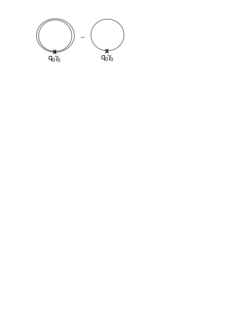
FIG. 1.: Schematic representation of $w$, eq. (11). The simple and double line represent the neutrino propagator, in the matter-free vacuum and in the vacuum of the interacting medium, respectively.

Using the notation

$$\sum\!\!\!\!\!\!\!\int_{n_{\pm}}\ \equiv\ \sum_{j_{z},l,...}\int dE_{n_{\pm}}\$$

and from the definition

$$S_{F}(x,y)\gamma_{0} = \theta(x^{0}-y^{0})\sum\!\!\!\!\!\!\!\int_{n_{+}}\Psi_{n_{+}}(\vec{x})\Psi^{{\dagger}}_{n_{+}}(\vec{y})\,e^{-iE_{n_{+}}(x^{0}-y^{0})}$$ (12)

$$- \theta(y^{0}-x^{0})\sum\!\!\!\!\!\!\!\int_{n_{-}}\Psi_{n_{-}}(\vec{x})\Psi^{{\dagger}}_{n_{-}}(\vec{y})\,e^{-iE_{n_{-}}(x^{0}-y^{0})}\ ,$$ (13)

where $E_{n_{-}}$ ($E_{n_{+}}$) is the negative (positive) energy of the eigenstate: $H\Psi_{n_{\pm}}=E_{n_{\pm}}\Psi_{n_{\pm}}$, $w(\vec{x})$ can be rewritten [14] as:

$$w(\vec{x})=\sum\!\!\!\!\!\!\!\int_{n_{-}}E_{n_{-}}\Psi^{{\dagger}}_{n_{-}}(\vec{x})\Psi_{n_{-}}(\vec{x})-\sum\!\!\!\!\!\!\!\int_{n_{-}}E^{(0)}_{n_{-}}\Psi^{{\dagger}(0)}_{n_{-}}(\vec{x})\Psi^{(0)}_{n_{-}}(\vec{x})\ ,$$ (14)

where $(0)$ refers to the matter-free vacuum and where we have taken the limit $y^{0}\to x^{0}$ with $y^{0}>x^{0}$. Taking the average of the limits $y^{0}\to x^{0}$ with $y^{0}>x^{0}$ and $y^{0}\to x^{0}$ with $y^{0}<x^{0}$, as done in [6], would lead to:

$$w_{sym}(\vec{x}) = \frac{1}{2}\sum\!\!\!\!\!\!\!\int_{n_{-}}E_{n_{-}}\Psi^{{\dagger}}_{n_{-}}(\vec{x})\Psi_{n_{-}}(\vec{x})-\frac{1}{2}\sum\!\!\!\!\!\!\!\int_{n_{-}}E^{(0)}_{n_{-}}\Psi^{{\dagger}(0)}_{n_{-}}(\vec{x})\Psi^{(0)}_{n_{-}}(\vec{x})$$ (15)

$$- \frac{1}{2}\sum\!\!\!\!\!\!\!\int_{n_{+}}E_{n_{+}}\Psi^{{\dagger}}_{n_{+}}(\vec{x})\Psi_{n_{+}}(\vec{x})+\frac{1}{2}\sum\!\!\!\!\!\!\!\int_{n_{+}}E^{(0)}_{n_{+}}\Psi^{{\dagger}(0)}_{n_{+}}(\vec{x})\Psi^{(0)}_{n_{+}}(\vec{x}).$$ (16)

The states are normalized in such a way that the two densities of states $\rho(E)$, with and without the star (free case), coincide in the asymptotic region $|\vec{x}|\to\infty$ so that $w(|{\vec{x}}|\to\infty)=0$.

For later use let us just remind the reader that the same result (14) may be obtained from the time Fourier-transformed propagator:

$$\tilde{S}_{F}(\vec{x},\vec{y},q^{0})\gamma_{0}=i\ \sum\!\!\!\!\!\!\!\int\ \frac{\Psi_{n_{+}}(\vec{x})\Psi^{{\dagger}}_{n_{+}}(\vec{y})}{q^{0}-E_{n_{+}}+i\epsilon}+\frac{\Psi_{n_{-}}(\vec{x})\Psi^{{\dagger}}_{n_{-}}(\vec{y})}{q^{0}-E_{n_{-}}-i\epsilon}.$$ (17)

The result (14) is obtained from (17) by integrating $-q^{0}\,S_{F}(\vec{x},\vec{y},q^{0})/(2\pi)$ on the complex $q^{0}$ plane, by closing the contour on the upper half. Obviously an appropriate choice for the $i\epsilon$ convention is crucial here, as discussed at length in [10]. It is also clear that formula (14) leads to much simpler calculations than the direct calculation of the loop in (11).

Obtaining the weak self-energy of the finite neutron star is equivalent to calculating the neutrino propagation in a background of neutron fields density with a border. We did that analytically in $(1\ +\ 1)$ dimensions with a sharp border, and in $(3\ +\ 1)$ dimensions with a flat border. The spherical symmetry has been studied both analytically and numerically.

III The toy example of $(1\ +\ 1)$ dimensions

Working directly with eq. (11) requires an interacting Feynman propagator that takes the existence of a border into account. Doing this in $(3\ +\ 1)$ dimensions is a big task.

It is feasible and theoretically fruitful to perform the analytical calculation of eq. (11) in $(1\ +\ 1)$ dimensions as a toy model. The knowledge extracted from that study will help us face the $(3\ +\ 1)$ realistic case by using the general formalism anticipated in section II. We will now summarize the ($1\ +\ 1$)-dimensional results presented in more detail in [10].

The ($1\ +\ 1$)-dimensional toy model is presented in ref. [10]. We will summarize the computation and the result in order to extract useful information for the more realistic case.

We consider $(1\ +\ 1)$ massless fermion Feynman propagators in a space with two regions separated by a border. The two regions, inside and outside the star, have different fermion dispersion relations, as seen in eq. (5).

For simplicity, we consider only one sharp border located at $z=0$ and use an effective neutrino Lagrangian, which summarizes the interaction with the neutrons [15]:

$${\cal L}_{\mathrm{eff}}=i{\overline{\nu}}(z)\hbox to0.0pt{/\hss}\partial\nu(z)-b\theta(z){\overline{\nu}}(z)\gamma^{0}\nu(z)\ \ ,$$ (18)

where $b$ is given by eq. (6). The details of the computation of the interacting propagator can be found in ref. [10]. In momentum space, the propagator can be written as follows:

$$\begin{array}[]{l}S_{F}(q^{f},q^{i})=2\pi\delta\left(q_{z}^{f}-q_{z}^{i}\right){i\over(\hbox to0.0pt{/\hss}q_{>})^{*}}\ +\ {b\over 2}\ {1\over q_{z}^{f}-q_{z}^{i}+i\varepsilon}\\ \times\left\{{1\over(\hbox to0.0pt{/\hss}q_{>}^{i})^{*}}\gamma^{0}{1\over\hbox to0.0pt{/\hss}q_{<}^{f}}\left(1+\mbox{sign}(q_{0})\alpha_{z}\right)\right.\left.+{1\over(\hbox to0.0pt{/\hss}q_{>}^{f})^{*}}\gamma^{0}{1\over\hbox to0.0pt{/\hss}q_{<}^{i}}\left(1-\mbox{sign}(q_{0})\alpha_{z}\right)\right\}\ \ ,\end{array}$$ (21)

where:

$${1\over\hbox to0.0pt{/\hss}q_{<}}={1\over\hbox to0.0pt{/\hss}q}={\hbox to0.0pt{/\hss}q_{<}\over q_{<}^{2}+i\varepsilon}\ \mbox{with}\ \ \left(q_{<}\right)^{\mu}=q^{\mu}=(q_{0},{\vec{q}})\ \ ,$$ (22)

$${1\over(\hbox to0.0pt{/\hss}q_{>})^{*}}={\hbox to0.0pt{/\hss}q_{>}\over q_{>}^{2}+is\varepsilon}\ \mbox{with}\ \ \left(q_{>}\right)^{\mu}=(q_{0}-b,{\vec{q}})\ \ ;$$ (23)

with $s=\mbox{sign}(q_{0})\mbox{sign}(q_{0}-b)$, and $\alpha_{z}=\gamma^{0}\gamma^{1}$. The sign $s$ results from the appropriate Feynman boundary conditions and from the right choice of the zero energy level. It gives an adequate time convention. We should emphasize that the propagator (21) is infrared-safe, all the $\hbox to0.0pt{/\hss}q$’s in the denominators being regularized by Feynman’s prescription for the distribution of the propagator poles in the complex-$q_{0}$ plane[10].

The expression for $1/(\hbox to0.0pt{/\hss}q)^{*}$, given by eq. (23), can be appropriately rewritten as

$${i\over(\hbox to0.0pt{/\hss}q_{>})^{*}}=i\left\{{1\over\hbox to0.0pt{/\hss}q_{>}}+2\pi i\hbox to0.0pt{/\hss}q_{>}\delta\left(q_{>}^{2}\right)\theta(-q_{0})\theta(q_{0}-b)\right\}\ .$$ (24)

In ref. [10], we have demonstrated that the main contribution to the weak self-energy comes from the first term of the propagator (21). We thus identified the expression given in
eq. (24) with the one for the effective propagator, which takes into account the “bulk” of the neutron star. As a matter of fact, the effective propagator for the infinite star [4] coincides with the propagator (24), except for the time convention introduced by the proper boundary conditions, responsible for the second term in the l.h.s. of eq. (24). This term is nothing else than the condensate contribution, i.e. the Pauli blocking effect of the neutrinos trapped into the star by the attractive potential. In refs. [4] and [8], the same condensate term in the l.h.s. was introduced by hand. Equations (23) and (24) give a confirmation of the idea proposed in refs. [4] and [15]: the condensate is a consequence of the existence of a border.

The condensate is physically understandable. As we have tuned the level of the Dirac sea (see eq. (5)) outside the star (to the left), and as our states extend over all space, far inside the star (to the right), the level corresponds to filling a Fermi sea above the bottom of the potential $b<q_{0}<0$. This obviously induces a Pauli blocking effect and eq. (5) anticipates this result: $|b|$ is a lower bound for the momentum of the positive-$q_{0}$ states.

Now, with the computation of the propagator, it is easy to calculate the weak self-energy density $w(z)$ for this ($1\ +\ 1$)-dimensional star by following eq. (11). Some details about this rather cumbersome calculation may be found in [10]. It is worth while emphasizing that the vanishing result (25) for the border contribution requires the change in the order of integration in the momentum space over the variables $q_{0},q_{z}^{i}$ and $q_{z}^{f}$. The latter is only possible in the framework of an implicit ultraviolet regularization scheme. As a matter of fact, the choice of a certain order of integration over the variables is an ultraviolet regularization method. By integrating over the momenta we found that this difference vanishes exactly:

$$w(z)=0\ \ .$$ (25)

This vanishing interaction energy in $(1\ +\ 1)$ dimensions has a simple physical explanation: the presence of the border does not disturb the wave functions (up to a phase). There is a one-to-one correspondence of the negative-energy states in the two media $z<0$ and $z>0$, and by interchanging the sum and integral as an ultraviolet regularization procedure, each term in eq. (14) vanishes exactly. In other words, massless propagating neutrinos are not reflected by the border of a $(1\ +\ 1)$ star, and the probability density is not affected by the border either.

The use of eq. (14) allows a trivial generalization of the vanishing result (25) in $(1\ +\ 1)$ dimensions to more complicated structures, for example a star with two sharp borders or, still better, to a continuously varying neutron density, as long as the density vanishes asymptotically outside the star.

IV Flat border in $(3\ +\ 1)$ dimensions

The computation of the neutrino loops (fig. 1) in the $(3\ +\ 1)$-dimensional case, with a finite star, as was done in the preceding section for $(1\ +\ 1)$ dimensions, is technically rather difficult, if only because the neutrino propagators are not simple. In the preceding section we have seen that the use of eq. (14) simplified the calculation a lot, reducing it practically to triviality in the latter case. We will therefore stick to it in the $(3\ +\ 1)$ case.

We might have faced the $(3\ +\ 1)$-dimensional problem analytically with interacting propagators and the approach that led to eq. (11), by using a simplifying assumption: the influence of the border can be reasonably neglected if the weak energy density is computed far inside the star. This amounts to considering a star large enough for the contribution of the bulk effective propagator (24) to be the main one. In other words, it would amount to assuming an infinite star but taking into account the existence of a matter-free vacuum infinitely far from the star centre. This matter-free vacuum allows us to fix the zero energy level, and consequently the adequate time convention for the effective propagator [10].

The latter calculation for the infinite star has indeed already been performed in our previous work [4]. There, $w(\vec{x})$ was computed using the Schwinger–Dyson expansion of
eq. (16) in [4] and the Pauli–Villars procedure as a means of regularization. As already noted in the introduction and in ref. [10], a pole ($q_{0}=|\vec{q}|+b$, in the case $|\vec{q}|<b$) has been forgotten (see fig. 1 in [10]) in the analytic continuation, which led to a wrong non-null result for $w(\vec{x})$ when the neutrino condensate effect was added by hand. This happened because we did not use the $i\epsilon$ prescription correctly: it had to be imposed in the propagators; this was already corrected in ref. [10]. Taking into account the results from refs. [4] and [10], we can conclude that the weak self-energy is null for an infinite stationary star. It should be repeated that following the correct $i\epsilon$ prescription, when using propagators, is equivalent to taking the zero energy level for the states by matching to the free states far outside the star. Of course the definition of the zero energy level is essential when using eq. (14), as we shall now do.

The null result for the $(3\ +\ 1)$-dimensional infinite star is a consequence of neglecting the existence of border effects. Now, before focusing on the spherical problem and in order to estimate the border effect, we concentrate on the geometrically easier problem: matter-free and neutron vacua separated by a flat border . For simplicity, the plane $z=0$ is assumed to be the flat border. The application of the approach resulting in eq. (14) requires a complete set of eigenfunctions for the Hamiltonian with the flat border. These eigenfunctions should be normalized following the same criteria as previously presented in section II: they asymptotically behave as plane waves far outside the star, in the sense that they provide, far outside the star, the same probability and energy density as the free plane waves (solutions without a star): $w(z=-\infty)=0$. This condition is imposed inside each Hilbert subspace with energy $E\in[E,E+dE]$.

Following [16], we obtain the following set of negative energy eigenfunctions:

$$\psi^{\mathrm{free}}_{n_{-}}(x) = N_{n_{-}}\left[\left(e^{ik_{i}^{<}x}v_{h}(\vec{k}_{i}^{<})+e^{ik_{r}^{<}x}{\cal R}v_{h}(\vec{k}_{i}^{<})\right)\ \theta(-z)\right.$$ (26)

$$+ \left.e^{ik_{t}^{>}x}(1+{\cal R})v_{h}(\vec{k}_{i}^{<})\ \theta(z)\right]$$ (27)

$$\psi^{\mathrm{mtt}}_{n_{-}}(x) = N_{n_{-}}\left[e^{i\vec{k}^{<}_{r}x}(1+{\cal J})v_{h}(\vec{k}^{>}_{mi})\theta(-z)\right.$$ (28)

$$+ \left.\left(e^{ik_{mi}^{>}x}v_{h}(\vec{k}_{mi}^{>})+e^{ik_{t}^{>}x}{\cal J}v_{h}(\vec{k}_{mi}^{>})\right)\ \theta(z)\right]\ \ ,$$ (29)

where they are directly related to incoming wave packets, the first coming from the free vacuum and the second one from the matter vacuum; $n_{-}$ labels the negative-energy eigenstate, $n_{\pm}=(\pm|E|,\vec{k}_{p},h=-1)$; $\vec{k}_{p}$ stands for the projection of the momentum on the flat border, and $h$ is the negative helicity of standard neutrinos; $N_{n_{-}}$ is the appropriate normalization factor. We also have $k^{>}=(|E|,\vec{k}^{>})$, $k^{<}=(|E|,\vec{k}^{<})$, and

$$\vec{k}_{i}^{<}=(k_{x},k_{y},k_{z}^{<})\ , \vec{k}_{r}^{<}=(k_{x},k_{y},-k_{z}^{<})\ ,$$ (30)

$$\vec{k}_{t}^{>}=(k_{x},k_{y},(k_{z}^{>})^{*})\ , \vec{k}_{mi}^{>}=(k_{x},k_{y},-k_{z}^{>})\ ;$$ (31)

the $z$-components of the momentum are defined as

$$k_{z}^{<} = +\sqrt{E^{2}-\vec{k}_{p}^{2}}$$ (32)

$$k_{z}^{>} = +\sqrt{(|E|-|b|)^{2}-\vec{k}_{p}^{2}}\ .$$ (33)

The reflection coefficients $\cal{R}$ and $\cal{J}$ can be computed following, for instance, the work of Gavela et al. [16], we find: ${\cal R}=-{\cal J}=R_{0}\vec{\alpha}\hat{k}_{p}$, where $\hat{k}_{p}$ is the unitary vector in the direction of the transverse momentum $\vec{k}_{p}$, and $\vec{\alpha}=\gamma^{0}\vec{\gamma}$; $R_{0}$ is given by:

$$R_{0}={2|b||\vec{k}_{p}|\over(k_{z}^{<}+k_{z}^{>})^{2}-b^{2}}\ \ .$$ (34)

If we consider a neutrino outside the star, with four-momentum $(|E|,\vec{k}^{<})$, it can easily be seen that, for $|E|-|b|<|\vec{k}_{p}|<|E|$, the matching condition generates a momentum inside the star with an imaginary component, $k_{z}^{>}=+i\sqrt{\vec{k}_{p}^{2}-(|E|-|b|)^{2}}$. Thus, a plane wave far outside the star in the above-mentioned parameter range generates a damped wave inside. We have, in other words, a non-penetrating wave. This is a crucial fact, because the probability density of waves inside and outside the star will be modified in a different way. It will be seen that the non-zero result for the weak self-energy, in both the flat and the spherical border cases, is dominated by the effect of these non-penetrating waves.

Following Gavela et al., we can be sure that the only negative-energy non-penetrating solution, once $n$ is fixed, is the first eigenstate of eqs. (29). Nevertheless, when transmission occurs, both eigenstates are needed to span the whole eigenspace. It can be seen that
eq. (29) appears to be a complete set of eigenfunctions [16], [17].

The normalization constants are chosen such that the probability density is asymptotically equal to the free one. For a given energy this can only be achieved on average up to an oscillating term that will be considered as a negligible local fluctuation. This normalization convention will reach its unambiguous meaning in the next section. There, the asymptotic density of the solutions far outside the star is tuned to the one in the free vacuum. This asymptotic region is taken to fix the normalization because it extends to infinity while the star occupies a limited region. Applying then eq. (14), we obtain the following weak energy density per energy:

$${\partial w\over\partial|E|}(z)=-{4\pi\over(2\pi)^{3}}|E|^{3}\left\{\Gamma(E,z)-\Gamma^{0}(E,z)\right\}\ ,$$ (35)

where $\Gamma^{0}(E,z)=1$, for free plane waves; $\Gamma(E,z)$, for instance in the region $|E|>|b|$, can be written as:

$$\Gamma(E,z)=\theta(-z)\ +\ \gamma(E)\theta(z)\ \ ,$$ (36)

where

$$\gamma(E)=\int_{0}^{1-|b^{*}|}dx{x\over\sqrt{1-x^{2}}}\ {1+{R^{*}_{0}\over 1+(R^{*}_{0})^{2}}x\over 1-{R^{*}_{0}\over 1+(R^{*}_{0})^{2}}{x\over 1-|b^{*}|}}\ \ .$$ (37)

The parameter $b^{*}$ is the dimensionless quantity $b/|E|$, and $R^{*}_{0}$ is the same function $R_{0}$ as given by eq. (34), expressed in terms of the variable $x=|\vec{k}_{p}|/|E|$ and of the parameter $b^{*}$. It is easy to see that $R_{0}$ is a real quantity, except for the non-penetrating waves, the result $|R_{0}|^{2}=1$ being satisfied in the latter case. It is important to insist on the fact that the local fluctuations originated by the interference of incident and reflected waves have been neglected in both regions, $z>0$ and $z<0$. The fact that these fluctuations contribute in a negligible way can be easily seen by performing the appropriate normalization of the eigenstates in a certain box. The contribution of the damped waves inside the star has also been neglected. That is why we integrate only for penetrating waves to obtain the function $\gamma(E)$, i.e. the reason of the upper bound in eq. (37), which implies that $R_{0}$ is always real in the l.h.s. of eq. (37). The latter damped waves occupy a thin layer inside the star and are necessary to make the probability density on the border continuous. A similar effect will be discussed in the following section for the spherical case.

In order to show the dominance of the effect of the non-penetrating waves, which is the main aim of this planar computation, the weak energy density (35) will be compared with a naive estimate of the one coming from non-penetrating waves: integrating simply the plane wave density in the two regions summed over all the allowed momenta in both $k_{z}=\sqrt{E^{2}-|\vec{k}_{p}|^{2}}$ for $z<0$ and $k_{z}=\sqrt{(|E|-|b|)^{2}-|\vec{k}_{p}|^{2}}$ for $z<0$, we obtain

$$\gamma^{S}(E)=\left({|E|-|b|\over|E|}\right)^{2}\ .$$ (38)

Equation (38) results from computing separately the density of states in the star and in the free vacua, the eigenstates in these vacua being obtained for translationally invariant Hamiltonians, which do not generate reflection on the border. The difference between $\gamma^{S}(E)$ and $\gamma(E)$ is precisely due to this neglecting of reflection. The result (38) only accounts for the fact that certain eigenstates, being allowed in the free vacuum, are not inside the star. There is an obvious one-to-one correspondence between these eigenstates and the ones for the untranslational-invariant Hamiltonian (18), which we called non-penetrating waves.

In fig. 2, the functions $\gamma(E)$ and $\gamma^{S}(E)$ have been plotted.

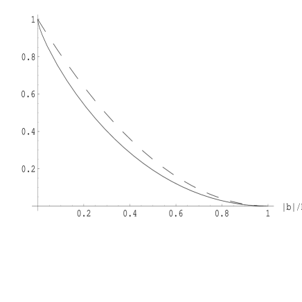
FIG. 2.: Plots of $\gamma(E)$ (dashed line) and $\gamma^{S}(E)$ (solid line), defined in the text, as a function of $|b|/|E|$.

The small difference between the two curves in fig. 2 shows that the dominant effect of the border comes from the non-penetrating waves. This result will be confirmed in the next section. A few comments are in order here. First, the new feature in the $(3\ +\ 1)$-dimensional case with respect to the $(1\ +\ 1)$ one is that the non-trivial neutrino refraction index not only bends the penetrating waves and induces a reflection, but also, beyond the limiting angle, induces total reflection. This well-known phenomenon, acting here on the negative energy states, induces the dominant contribution to the star weak self-energy density. It must be stressed that this effect of non-penetrating waves is utterly unrelated to any Pauli blocking effect from the neutrino condensate inside the star. Indeed, as we have shown in the $(1\ +\ 1)$ case, in which the condensate exists, its effect is precisely to equate the energy density inside the star to the one outside. On the other hand, the non-penetrating waves are reflected, not because of some states, which are already occupied, but because they tend to occupy states that simply do not exist, with an imaginary momentum. Finally, let us insist that
eqs. (35) and (37) imply that the border effect discovered here is a volume effect, i.e. it affects the energy density by an almost constant amount in the whole volume occupied by the star. This result is rather unexpected, a border effect being thought to act only on the surface. Of course it relies on the hypothesis that the wave packets extend coherently over the whole star. As will be discussed in section VI, such a hypothesis is perfectly sound for low-energy neutrinos.

V Realistic star: spherical 3-d

We study a massless neutrino in the presence of an external symmetric static electroweak potential of finite range due to the interaction with the neutrons of the star. In order to calculate the weak self-energy $\int d^{3}r\ w(\vec{r})=\int d^{3}r\ (\langle\hat{0}|{\cal H}(0)|{\hat{0}}\rangle-\langle{0}|{\cal H}_{0}(0)|{0}\rangle)$, which is nothing else than the difference (14) integrated over space, we need to use the spherical Bessel functions [18] as a basis for the solutions of the Dirac equation. The effect of the static neutrons is summarized in the spherically symmetric square-well potential of depth $b<0$ ($b\sim-20$ eV):

$$V(r)=\left\{\begin{array}[]{ll}\ b<0&{\mathrm{for}}\ \ r\leq R\\ \ 0&{\mathrm{for}}\ \ r>R\end{array}\right.$$ (41)

$R$ being the radius of the star.
¿From the effective Lagrangian of eq. (9),

$${\cal{L}}_{\mathrm{eff}}={\overline{\psi}}\left(i\partial\!\!\!/-V(r)\gamma_{0}\right)\ \psi(r)\ ,$$ (42)

the Dirac equation is:

$${\vec{\alpha}}\cdot{\vec{p}}\ \psi({\vec{r}})=\left(E-V(r)\right)\psi({\vec{r}})\ ,$$ (43)

where

$$\vec{\bf\alpha}=\left(\begin{array}[]{cc}0&\vec{\bf\sigma}\\ \vec{\bf\sigma}&0\end{array}\right)\ .$$

Turning the kinetic energy operator $\vec{\alpha}\cdot{\vec{p}}$ into spherical polar coordinates, we obtain the eigensolutions :

$$\psi_{\kappa,m}({\vec{r}})=N\ \left(\begin{array}[]{l}\ u_{1}(r)\ \chi_{\kappa}^{m}(\theta,\phi)\\ iu_{2}(r)\ \chi_{-\kappa}^{m}(\theta,\phi)\end{array}\right)\ ,$$ (46)

where $N$ is a normalization factor and $\chi_{\pm\kappa}^{m}(\theta,\phi)$ are the two-spinors [19] written in terms of the spherical harmonics $Y_{l}^{m}$ and spin $1/2$ eigensolutions $\chi_{{1\over 2},\mu_{s}}$:

$$\chi_{\kappa>0}^{m}(\theta,\phi)={\displaystyle{\sum_{\mu,\mu_{s}}\left\langle\kappa\mu\frac{1}{2}\mu_{s}{\bigg{|}}\left(\kappa-\frac{1}{2}\right)m\right\rangle{Y}_{\kappa}^{\mu}(\theta,\phi)\chi_{{1\over 2},\mu_{s}}}}=\,\left(\begin{array}[]{c}-\sqrt{\frac{\kappa-m+\frac{1}{2}}{2\kappa+1}}Y_{\kappa,m-\frac{1}{2}}\\ \sqrt{\frac{\kappa+m+\frac{1}{2}}{2\kappa+1}}Y_{\kappa,m+\frac{1}{2}}\end{array}\right),$$ (49)

$$\!\!\chi_{\kappa<0}^{m}(\theta,\phi)\!=\!\sum_{\mu,\mu_{s}}\left\langle(-\kappa-1)\mu\frac{1}{2}\mu_{s}{\bigg{|}}\left(-\kappa-\frac{1}{2}\right)m\right\rangle\!{Y}_{-\kappa-1}^{\mu}(\theta,\phi)\chi_{{1\over 2},\mu_{s}}\!=\!\left(\!\begin{array}[]{c}\sqrt{\frac{-\kappa+m-\frac{1}{2}}{-2\kappa-1}}Y_{-\kappa-1,m-\frac{1}{2}}\\ \sqrt{\frac{-\kappa-m-\frac{1}{2}}{-2\kappa-1}}Y_{-\kappa-1,m+\frac{1}{2}}\end{array}\!\right)$$ (52)

Here $\chi_{\pm|\kappa|}^{m}(\theta,\phi)$ are eigensolutions of $J^{2}$, $J_{z}$, $L^{2}$ and $S^{2}$, where $\vec{J}=\vec{L}+\vec{S}$, $J_{z}$, $\vec{L}$ and $\vec{S}$ are respectively the total angular momentum, its projection along the $z$-axis, the orbital angular momentum and the spin angular momentum verifying the eigenvalue equations:

$$\left\{\begin{array}[]{l}(\vec{\bf\sigma}\cdot\vec{L}+1)\ \chi_{\pm|\kappa|}^{m}(\theta,\phi)\ =\ \mp|\kappa|\chi_{\pm|\kappa|}^{m}(\theta,\phi)\ ,\\ {J_{z}}\chi_{\pm|\kappa|}^{m}(\theta,\phi)\ =\ m\chi_{\pm|\kappa|}^{m}(\theta,\phi)\ ,\ \ -J\leq m\leq+J\ ,\\ |\kappa|=(1,2,...)\ ,\ \ |\kappa|=J+1/2\ .\end{array}\right.$$ (56)

With this notation, we can easily check that the two chirality states are described by the same spinor of eq. (46):

$$\psi^{m}_{\kappa_{L,R}}={\frac{1}{2}}\ (1\ \mp\ \gamma_{5}\ )\psi^{m}_{|\kappa|}\ ,$$ (57)

the positive and the negative values of $\kappa$ being related through the relation:

$${\displaystyle{i\ \gamma_{5}\ \psi^{m}_{-|\kappa|}=\psi^{m}_{|\kappa|}}}\ .$$ (58)

It then suffices to compute $\psi^{m}_{\kappa}$ for positive values of $\kappa$, use eq. (58) for the negative values of $\kappa$ and then get the left-chirality neutrino state using eq. (57). Let us from now on write the positive $\kappa$’s as $\kappa\equiv l=1,\ 2,\ 3,....$, with $J=l-1/2$ (see eq. (49)).

The radial functions $u_{1,2}$ defined in eq. (46) verify the following coupled differential equations:

$${d\over dr}\left(\begin{array}[]{l}r\ u_{1}(r)\\ r\ u_{2}(r)\end{array}\right)=\left[\begin{array}[]{cc}\ {-l\over r}&(E-V(r))\\ -(E-V(r))&{l\over r}\end{array}\right]\ \ \left(\begin{array}[]{l}r\ u_{1}(r)\\ r\ u_{2}(r)\end{array}\right)\ .$$ (65)

Now, decoupling the equations and using eq. (41) and the fact that the solution must be regular in the centre of the core, i.e. $r\to 0$, we get:

$$\left\{\begin{array}[]{l}u_{1}(r)\ =\alpha\big{[}\ j_{l}\left(k\ r\right)\ \theta(R-r)+(B\ j_{l}(E\ r)+C\ y_{l}(E\ r))\ \theta(r-R)\big{]}\\ u_{2}(r)\ =\alpha\big{[}\ j_{l-1}\left(k\ r\right)\ \theta(R-r)+(B\ j_{l-1}(E\ r)+C\ y_{l-1}(E\ r))\ \theta(r-R)\big{]}\ ,\end{array}\right.$$ (68)

where we define

$$k=E-b,$$ (69)

$$\alpha={1\over\sqrt{B^{2}+C^{2}}}\ ;$$ (70)

$B,\ C$ being integration coefficients to be fixed from the matching condition at the surface. The factor $\alpha$ will be justified below to guarantee the good asymptotic behaviour of functions $u_{1,2}(r)$. The functions $j_{l}$ and $y_{l}$ are the spherical Bessel functions of the first and second kind. In the inner region, the solution can be written only in terms of $j_{l}$ because the wave functions have to be regular at the origin and the $y_{l}(\rho)$’s are not (see eq. (92)).

According to eq. (14), we are going to use only negative energy states and thus negative arguments for these Bessel functions ($E,k<0$) and the following relations are helpful:

$$j_{l}(\rho)=(-1)^{l+1}j_{l}(-\rho)\ ,\qquad y_{l}(\rho)=(-1)^{l}y_{l}(-\rho)\ .$$ (71)

The solutions $u_{1,2}$ have been written in the form (68) in order to match, up to a phase, the free solutions as $r\to\infty$, where the asymptotic behaviour of the Bessel functions is:

$$j_{l}(\rho){\displaystyle{\ \stackrel{{\scriptstyle\sim}}{{{}_{\rho\to\infty}}}}}\ \sin\left(\rho-\frac{l\pi}{2}\right){\bigg{/}}\rho\ ,\qquad y_{l}(\rho){\displaystyle{\ \stackrel{{\scriptstyle\sim}}{{{}_{\rho\to\infty}}}}}\ \cos\left(\rho-\frac{l\pi}{2}\right){\bigg{/}}\rho\ .$$ (72)

This behaviour implies the one followed by our solutions $u_{1,2}$:

$$u_{1}(E\ r) {\displaystyle{\ \stackrel{{\scriptstyle\sim}}{{{}_{r\to\infty}}}}} \ \sin\left(E\ r-\frac{\pi l}{2}+\phi\right){\bigg{/}}E\ r\ ,$$ (73)

$$u_{2}(E\ r) {\displaystyle{\ \stackrel{{\scriptstyle\sim}}{{{}_{r\to\infty}}}}} \ \cos\left(E\ r-\frac{\pi l}{2}+\phi\right){\bigg{/}}E\ r\ ,$$ (74)

$${\mathrm{where}}\ \qquad\qquad\qquad\ \phi = \arctan(C/B)\ .$$ (75)

Needless to say that in the absence of the star ($b=0$), $\alpha=1$ and the spherical solutions fit exactly the free ones, in the asymptotic region $r\to\infty$.

Both inner and outer solutions must join at $r=R$, and this matching fixes the coefficients $B$ and $C$ as follows:

$$\begin{array}[]{l}B\ =\ {\displaystyle{{j_{l}(k\ R)\ y_{l-1}(E\ R)-j_{l-1}(k\ R)\ y_{l}(E\ R)\over j_{l}(E\ R)\ y_{l-1}(E\ R)-j_{l-1}(E\ R)\ y_{l}(E\ R)}}}\ ,\\ \\ C\ =\ {\displaystyle{{j_{l-1}(k\ R)\ j_{l}(E\ R)-j_{l-1}(E\ R)\ j_{l}(k\ R)\over j_{l}(E\ R)\ y_{l-1}(E\ R)-j_{l-1}(E\ R)\ y_{l}(E\ R)}}}\ .\end{array}$$ (79)

Finally, in order to fix the solutions definitively, we need to calculate the normalization factor $N$ by following the asymptotic normalization convention already introduced in the previous section: we impose the probability density to be asymptotically equal to the free one. Since we have fitted $\alpha$ to make the solutions with $b\neq 0$ coincide, up to a phase, with those of the free case ($b=0$) when $r\to\infty$, we need to compute $N$ only for the free case. In the latter case, $b=0,\alpha=1$, the Hilbert space of spherical solutions is the one of the free plane waves ${1\over(2\pi)^{3}}e^{i\vec{p}\cdot\vec{r}}$. The solutions (see eq. (79)) reduce to

$$\psi^{m}_{l}({\bf r})=N\ \left(\begin{array}[]{l}j_{l}(E\ r)\ \chi_{l}^{m}(\theta,\phi)\\ ij_{l-1}(E\ r)\ \chi_{-l}^{m}(\theta,\phi)\end{array}\right)\ .$$ (80)

Now we compute the density of these states $\rho(E)$ in the Hilbert subspace corresponding to
$E\in[E,E+dE]$, by summing up all the quantum numbers and the angular degrees of freedom, while keeping the left chirality and spin fixed because we are counting the negative-energy and left-handed neutrino states. This gives the probability $\rho(E)dE={4\pi E^{2}\over(2\pi)^{3}}dE$. Using the relation [18]

$$\sum_{\mu=0}^{\infty}(2\mu+1)|j_{\mu}|^{2}=1\ ,$$ (81)

we obtain:

$$N=E/\sqrt{2\pi}\ .$$ (82)

Now that the solutions of the Dirac equation are known, we can calculate numerically $w(r)$, which can be written following eq. (14) as [14]:

$$w(\vec{r})=\int dE\ \sum_{l,m}E\ \left(\psi^{m}_{l}{\dagger}(\vec{r})\ \psi^{m}_{l}(\vec{r})-\psi^{m\ (0)}_{l}{\dagger}(\vec{r})\ \psi^{m\ (0)}_{l}(\vec{r})\right)\ ,$$ (83)

where the sum is over all the degrees of freedom of the negative-energy left-handed neutrinos and where the subscript $(0)$ refers to the matter-free solutions ($b=0$). The integration over the angular part and the summation over $m$ is direct, using eqs. (49) and (52), which lead to

$${\frac{1}{4\pi}}\int\ d\Omega\sum_{m}\chi{\dagger}_{\l}^{m}(\theta,\phi)\chi_{\l}^{m}(\theta,\phi)={(2J+1)\over 4\pi}={2l\over 4\pi}\ .$$ (84)

The weak self-energy density ($w(r)\equiv dW/dV={{{dW\over 4\pi r^{2}dr}}}$, $W$ being the total weak energy and $V$ the volume) is then simplified to (using the spherical symmetry);

$$w(r)=\int^{0}_{-\infty}dE\ {E^{3}\over 2\pi^{2}}\sum_{l}l(\rho_{l}(k,r)-\rho^{(0)}_{l}(E,r))\ ,$$ (85)

where we have defined

$$\begin{array}[]{l}\rho_{l}(k,r)=\alpha^{2}\left\{\left[j_{l}^{2}(k\ r)+j_{l-1}^{2}(k\ r)\right]\theta(R-r)\right.+\\ \left.\quad\quad\quad\ \ \ \left[(Bj_{l}(E\ r)+Cy_{l}(E\ r))^{2}+(Bj_{l-1}(E\ r)+Cy_{l-1}(E\ r))^{2}\right]\theta(r-R)\right\}\ ,\\ \rho_{l}^{(0)}(E,r)=j_{l}^{2}(E\ r)+j_{l-1}^{2}(E\ r)\ ,\end{array}$$ (89)

$k$ and $\alpha$ being given by eq. (70). We were not able to perform the summation over all the values $l$ and negative energies analytically. We then use numerical computations of the Bessel functions, and use some knowledge (see ref. [18]) about these functions in order to justify the truncation of these infinite summations in $l$, as will be explained now.

Let us define the function

$$f(E,r,l_{2})=\sum_{l=1}^{l_{2}}l(\rho_{l}(k,r)-\rho^{(0)}_{l}(E,r))\ ,$$ (90)

We have observed that for $r>R$ and fixed values of $E$ and $l_{2}$, the result becomes rather stable from $r\stackrel{{\scriptstyle>}}{{{}_{\sim}}}R$ up to $r\gg R$, while there is a sudden change when we pass the border $r=R$. When we integrate the density over $r$, the main contribution to (90) comes from inside the star, $r\in[0,R]$ and thus the effect is grossly proportional to the volume.

In order to understand these results qualitatively, a few remarks about the behaviour of Bessel functions are appropriate. The spherical Bessel functions are solutions of the differential equation:

$$\left({d^{2}\over d\rho^{2}}+k^{2}-{l(l+1)\over\rho^{2}}\right)(\rho j_{l})=0,\qquad\left({d^{2}\over d\rho^{2}}+k^{2}-{l(l+1)\over\rho^{2}}\right)(\rho y_{l})=0\ .$$ (91)

For $\rho$ large, say $\rho\sim\rho_{0}$, we may get a hint by replacing $1/\rho^{2}$ by $1/\rho_{0}^{2}$ in eq. (91).
For ${\displaystyle{k^{2}-{l(l+1)/\rho_{0}^{2}}<0}}$, i.e. $l\stackrel{{\scriptstyle>}}{{{}_{\sim}}}|k|\ \rho_{0}$, the solution $j_{l}$ ($y_{l}$) is a damped (exploding) exponential . This damping (explosion) is expressed by the well-known behaviour of the spherical Bessel functions $j_{l}$ and $y_{l}$ in the vicinity of the centre:

$$j_{l}(\rho){\displaystyle{\stackrel{{\scriptstyle\sim}}{{{}_{\rho\to 0}}}}}{\rho^{l}\over(2l+1)!!}\ \ ,\qquad y_{l}(\rho){\displaystyle{\stackrel{{\scriptstyle\sim}}{{{}_{\rho\to 0}}}}}{(2l+1)!!\over(2l+1)}\rho^{-(l+1)}\ .$$ (92)

For ${\displaystyle{k^{2}-{l(l+1)/\rho_{0}^{2}}>0}}$, - i.e. $l\stackrel{{\scriptstyle<}}{{{}_{\sim}}}|k|\ \rho_{0}$, the solution is an oscillating function as expressed by the asymptotic behaviour (72).

In practice the transition between these two asymptotic regimes is rather fast. In other words, the Bessel function $j_{l}(\rho)$ increases with $\rho$ at first as a power of $\rho$, then increases exponentially until a transition at $\rho=\sqrt{l(l+1)}$ where it becomes an oscillating function, see eq. (72). Spherical Bessel functions are not so different from

$$j_{l}^{ap}(\rho) = \ \theta(\rho-\sqrt{l(l+1)})\,\sin\left(\rho-\frac{l\pi}{2}\right){\bigg{/}}\rho,\quad\forall\rho,$$ (93)

$$y_{l}^{ap}(\rho) = \ \theta(\rho-\sqrt{l(l+1)})\,\cos\left(\rho-\frac{l\pi}{2}\right){\bigg{/}}\rho,\quad\rho-\sqrt{l(l+1)}>0.$$ (94)

The exploding part of $y_{l}$ is not described by eq. (94), but we do not care since, precisely from imposing regularity at the origin, the $y_{l}$’s only contribute to our solutions outside the star, eq. (68), where they are in their oscillating regime, as can be easily checked.

In the following we will use this approximation to guess the results and we will check numerically these guesses and estimate the corrections to these approximations. Such a strategy is necessary since we are totally unable to calculate numerically with the realistic value of $|b|R$, which is of the order of $\sim 10^{12}$. This would need computing up to angular momenta larger than $10^{12}$ ! In practice we have modestly limited ourselves to $|b|R\simeq 10$ and $|E|/b$ going up to $\simeq 100$. It is then mandatory to get a qualitative understanding of the results to be able to extrapolate them to the realistic values. Before going further, it is worth remarking that the function $j_{l}^{ap}$ defined in (94) verifies the saturation relation (81) at leading order in $1/(|k|r)$.

From (94) it seems that the summations on $l$ may be truncated at $l\stackrel{{\scriptstyle>}}{{{}_{\sim}}}|E|r$. In order to check this conjecture we will use the free case in which we know the exact solution. For the plane waves, the energy density $w_{p}$ due to left-handed negative-energy neutrinos is

$$w_{p}(r)=\int dE\ \frac{E^{3}}{2\pi^{2}}=\int dE\,\frac{E^{3}}{2\pi^{2}}\,\sum_{l=1}^{\infty}l\rho^{(0)}_{l}(E,r)\ ,$$ (95)

as can be directly computed from the plane wave functions, and also via the definition of $\rho^{(0)}_{l}$ in (89) with the help of relation (81). The integration over $E$ in eqs. (85) and (95) is of course divergent. We will come to this ultraviolet problem later, in section VI.

We have computed

$${dG_{p}\over dE}\equiv{\displaystyle{\int_{0}^{R}}}\ 4\pi r^{2}\ dr\frac{E^{3}}{2\pi^{2}}$$ (96)

and compared it with

$${dG\over dE}\equiv{\displaystyle{\int_{0}^{R}}}\ 4\pi r^{2}\ dr\frac{E^{3}}{2\pi^{2}}\sum_{l=1}^{l_{2}}l\rho^{(0)}_{l}(E,r)$$ (97)

in order to see the convergence of the summation. It is confirmed that the summation ${{\sum_{l=1}^{l_{2}}}}l\rho^{(0)}_{l}(E,r)$ is already very close to its limit $1$ as soon as $l_{2}>|E|\ R$. This can be seen in fig. 3, where we have plotted the absolute values of eqs. (96) and (97).

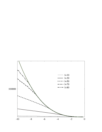
FIG. 3.: ${\left|dG\over dE\right|}$ in eq. (97) as a function of the energy expressed in units of $|b|$. The summation on $l$ goes from 1 to the value indicated on the figure, $r$ is integrated between $0$ and $R$ (the radius $R$ of the star has been fixed to $10|b^{-1}|$). The bold line represents the plane wave density ${\left|dG_{p}\over dE\right|}$ in eq. (96).

We have also checked that the summation in (90) saturates when $|E|\ r<l_{2}$.

The numerical computations show that $\alpha$, eq. (70), is quasi-independent of $l$ for
$l<|E-b|\ R$ and is verified for:

$$\alpha^{2}\stackrel{{\scriptstyle{\simeq}}}{{{}_{|E-b|R>l}}}\alpha_{t}^{2}\equiv\left({E-b\over E}\right)^{2}\,.$$ (98)

This result may be understood by the following argument. Using the approximation (94), the waves that do not vanish inside the star near the border have the form of a sine divided by $(k\ R)$. The corresponding ones, outside the star, are a combination of a sine and a cosine divided by $(E\ R)$. Taking the trigonometric functions to be of the same size on average, an obvious factor of $\alpha\simeq\alpha_{t}=|k/E|$ is needed for the matching at $R$ of the inside waves and the outside ones. Interestingly enough, this result leads, combined with (81), i.e. summing over all angular momenta, to an average energy density inside the star of

$$E(E-b)^{2}/(2\pi^{2})\ ^{\prime}$$ (99)

which is the energy multiplying the plane wave probability density, see eq. (95), but for a plane wave shifted by the potential $b$. This is reminiscent of eq. (38).

The validity of eq. (98) is shown in fig. 4, where we compare $\alpha$ to $\alpha_{t}$ for different values of the energy and the parameter $l$. We can see on this figure that $\alpha^{2}-\alpha^{2}_{t}$ is negligible in average, as long as the momentum $l$ verifies $l\ll|E-b|\ R$.

FIG. 4.: $\alpha^{2}-\alpha^{2}_{t}$ (see eqs. (98) and (70)) as a function of $l$, for different values of the energy. The star radius is $R=10b^{-1}$.

At this point, we now have a “naive” or “crude” formula for $w(r)$:

$$w_{crude}(r)\equiv\int dE\ {E\over 2\pi^{2}}\left((E-b)^{2}-E^{2}\right)\,\theta(R-r)\ ,$$ (100)

of course, this is a first approximation, the same as we had reached in the flat case (see section IV) from the function $\gamma^{S}(E)$, eq. (38).

The reason for this agreement between the flat case and the spherical one is easy to understand physically. It is related to the non-penetrating waves. Let us first consider the waves with $l<|E-b|\ R$. We have already argued that they are trigonometric functions divided by $|E-b|\ R$ ($|E|\ R$) inside (outside) the star. They are matched on the border. From that matching itself and their oscillating behaviour, their density has to match up to a large distance from the border. A different and crucial effect comes from the angular momenta

$$|(E-b)|\ R<l<|E|\ R\ .$$ (101)

In the trigonometric regime these waves are functions divided by $|E|\ R$ outside, while inside they are in the fast decreasing regime. The matching adjusts them for $r=R$, but, as $r$ decreases inside the star, they fall very fast. Essentially they are non-penetrating waves exactly analogous to the ones with $|E-b|<k_{p}<|E|$ in the previous section. Indeed, since $\vec{L}\simeq\vec{r}\times\vec{k}$, and noticing that the radial vector being perpendicular to the surface, its cross product with $\vec{k}$ is parallel to the surface, it becomes obvious that the inequality $|E-b|<k_{p}<|E|$ is equivalent to eq. (101).

We have thus seen qualitatively, and checked numerically, that the dominant contribution to $w(\vec{r})$ is due to non-penetrating waves in the spherical case as well as in the planar case.

The numerical check consisted in the following steps.
In the beginning, we compared:

$${dW\over dE}\equiv{\displaystyle{\int_{0}^{r_{max}}}}\ 4\pi r^{2}dr\ {E^{3}\over 2\pi^{2}}\sum_{l=1}^{l_{2}}l(\rho_{l}(k,r)-\rho^{(0)}_{l}(E,r))\ ,$$ (102)

for several values of $l_{2}$, $r_{max}$ being greater than the star radius $R$, with

$${dW_{crude}\over dE}\equiv{E\over 2\pi^{2}}\left((E-b)^{2}-E^{2}\right)\ 4\pi\ R^{3}/3\ .$$ (103)

In fig. 5, we have plotted eq. (102) as a function of the energy for several values of $l_{2}$ and compared with eq. (103). The integration over $r$ in eq. (102) has been done from $0$ to $r_{max}=3R$. This figure confirms that, as long as $|E|\ R<l_{2}$, there is no sizeable difference between the exact result (102) and the “crude” one (103). For higher values of $|E|\ R$, we must increase $l_{2}$ in order to take all the contributions into account.

FIG. 5.: ${\left|dW\over dE\right|}$ in eq. (102) as a function of the energy expressed in units of $|b|$. The summation on $l$ goes from 1 to the value indicated in the figure, $r$ is integrated between $0$ and $r_{\mathrm{max}}=30\ |b^{-1}|$ (the radius of the star has been fixed to $10|b^{-1}|$). The bold line represents the energy density ${\left|dW_{crude}\over dE\right|}$ in eq. (103).

After that, in order to check the corrections to our formula eq. (100) more accurately, we computed:

$$\begin{array}[]{l}\qquad{\displaystyle{{d\delta(r)\over dE}}}={\displaystyle{{d\delta_{in}\over dE}}}+{\displaystyle{{d\delta_{out}\over dE}}}\\ {\mathrm{where}}\\ \qquad{\displaystyle{{d\delta_{in}(r)\over dE}}}\equiv 4\pi r^{2}{E^{3}\over 2\pi^{2}}\left[{\displaystyle{\sum_{l=1}^{l_{2}}}}\left(\alpha^{2}-\alpha_{t}^{2}\right)l\left(j_{l}^{2}(k\ r)+j_{l-1}^{2}(k\ r)\right)\right]\theta(R-r)\\ {\mathrm{and}}\\ \qquad{\displaystyle{{d\delta_{out}(r)\over dE}}}\equiv 4\pi r^{2}{E^{3}\over 2\pi^{2}}\ {\displaystyle{\sum_{l=1}^{l_{2}}}}\ l\left[\alpha^{2}\left((Bj_{l}(Er)+Cy_{l}(Er))^{2}\right.\right.\\ +\left.\left.(Bj_{l-1}(Er)+Cy_{l-1}(Er))^{2}\right)-\rho^{(0)}(E,r)\right]\theta(r-R)\ .\end{array}$$ (110)

Here, we are subtracting from the exact formula the “crude” one, expanded in Bessel functions with the help of the constant factor $\alpha_{t}$. Indeed, from the plane wave expansion (95) and the definition of $\alpha_{t}^{2}$ (98), it is obvious that the term proportional to $\alpha_{t}^{2}$ in (110) sums up to the one proportional to $E(E-b)^{2}$ in (103) and that the term proportional to $E^{3}$ cancels the sum of the terms $\rho_{l}^{(0)}$. We have expanded the “crude” contribution into Bessel functions in order to minimize the error due to the truncation of the sum.

After having performed the integration over $r$:

$$\begin{array}[]{l}\qquad{\displaystyle{{d\Delta\over dE}}}={\displaystyle{{d\Delta_{in}\over dE}}}+{\displaystyle{{d\Delta_{out}\over dE}}}\\ {\mathrm{where}}\\ \qquad{\displaystyle{{d\Delta_{in}\over dE}}}={\displaystyle{\int_{0}^{R}}}\ dr\ {\displaystyle{{d\delta_{in}\over dE}}}\qquad{\mathrm{and}}\qquad{\displaystyle{{d\Delta_{out}\over dE}}}={\displaystyle{\int_{R}^{r_{max}}}dr\ {\displaystyle{{d\delta_{out}\over dE}}}\ ,}\end{array}$$ (114)

we compare in fig. 6 eqs. (102) and (114). We can see from the figure that the correction to our naive formula (100) is relatively very small and better for larger energies .

FIG. 6.: The dashed line represents ${\left|dW\over dE\right|}$ in eq. (102) and the solid line ${\left|d\Delta\over dE\right|}$ in eq. (114). They are functions of the energy expressed in units of $|b|$. The summation over $l$ was done from $1$ to $80$ and the integration over $r$ from $r=0$ to $r=30|b^{-1}|$ (the star radius being $R=10|b^{-1}|$).

The integration over $r$, where $r_{max}>R$, shows that

$${d\Delta_{in}\over dE}<0\ \ {\mathrm{and}}\ \ {d\Delta_{out}\over dE}>0,$$ (115)

which means that our crude estimate is an underestimate (overestimate) of the probability density inside (outside) the star. This fact is due to the tendency of the exact solution to provide a continuous matching on the border, while our “crude” formula has a jump. We shall discuss this in more detail. Moreover, we have found that this overestimate and underestimate approximately cancel as can be seen from fig. 7. Note that in this figure
(fig. 7), the summation over $l$ goes to $l_{2}=80$, the fluctuations that we see for $E<-8|b|$ are due to the truncation in the sum over $l$ when $|E|\ R>80$.

FIG. 7.: The horizontal axis represents the energy in units of $|b|$. The summation over $l$ has been performed from $1$ to $80$. For $E>8b$, the positive curve represents (eq. (114)) the contributions ${d\Delta_{out}}/{dE}$ of the exterior of the star, the negative curve the contributions $\frac{d\Delta_{in}}{dE}$ of the interior. For the exterior contribution, $r$ have been integrated from $R$ to $3R$, the star radius $R$ being fixed to $R=10|b^{-1}|$. An accurate cancellation of both pieces is seen. The oscillation seen for $E<8b$ is due to the truncation artefact.

Let us look in more detail into how the sudden jump of our naive formula (100) when crossing the border of the star is smoothed down into the exact result. There must be some layer in which the transition takes place. As we have already claimed, this layer is dominated by the functions in the domain of eq. (101). The width of the border effect depends directly on the speed of the falling-down of the Bessel functions in (101). If we use the fact that, for $l$ high enough, the spherical Bessel functions behave like $(|k|\ r)^{l}$ (see eq. (92)), we can try an estimate of the border effect, which gives the correction to our “naive” eq. (100). The mean value of $l$ inside the domain (101) is

$$l_{{\mathrm{mean}}}=R\ {\bigg{|}}\left(E-{\frac{b}{2}}\right){\bigg{|}}\ .$$ (116)

If we suppose that half of the jump occurs at $r=R_{-}\stackrel{{\scriptstyle<}}{{{}_{\sim}}}R$ in the interior of the star and the other half outside $r=R_{+}\stackrel{{\scriptstyle>}}{{{}_{\sim}}}R$, we can construct a term proportional to

$${dS(r)\over dE}\equiv\ 4\pi r^{2}{E^{3}\over 2\pi^{2}}\left[{\frac{1}{2}}(1-\alpha_{t}^{2})\left({r\over R}\right)^{2l_{{\mathrm{mean}}}}\theta(R-r)-{\frac{1}{2}}(1-\alpha_{t}^{2})\left({R\over r}\right)^{2l_{{\mathrm{mean}}}}\theta(r-R)\right]\ ,$$ (117)

which will have the role of smoothing the jump in our naive approximation formula eq. (100).

In order to confirm this effect, we have compared in fig. 8, for different values of the energy, ${dS/dE}$ with ${d\delta/dE}$.

FIG. 8.: The dashed line represents ${\displaystyle{{dS\over dE}}}$ in eq. (117) and the solid line ${\displaystyle{{d\delta\over dE}}}$ in eq. (110), as functions of the position $r$, in units of $|b^{-1}|$ (the radius of the star has been fixed to $R=10\ |b^{-1}|$) for different values of the energy. The summation over $l$ has been done from $1$ to $80$. The two lines are similar, confirming the validity of approximation (117), except for $E=10|b|$ where the truncation artefact dominates.

In fig. 8, we can see the agreement between the l.h.s. of eqs. (117) and (110), except for $E$ such that $|E|\ R\stackrel{{\scriptstyle>}}{{{}_{\sim}}}l_{2}$, where the truncation effects are important.

To have an estimate of the width $d$ in which the “joining” occurs, it suffices to write

$$\left(\frac{r}{R}\right)^{l_{{\mathrm{mean}}}}=\exp\left(l_{{\mathrm{mean}}}\log(\frac{r}{R})\right)\ ;$$ (118)

defining $d$ such that the probability decreases by a factor of $1/e$, we get

$$d=\frac{1}{|E-b/2|}\ .$$ (119)

From fig. 8, we can easily see that the larger $|E|$ is, the narrower the width of the joining layer is. This is clearly seen in fig. 8 a while in 8 b, beyond $E=8b$, the truncation effect comes into play, since $|E|\ R\stackrel{{\scriptstyle>}}{{{}_{\sim}}}l_{2}=80$.

VI discussion

We now have a qualitative understanding of the dominant contribution to the star mass correction due to the neutrino exchange. It doesn’t vanish when we consider the realistic $(3\ +\ 1)$-dimensional star, because of a border effect proportional to the volume of the star. It is ultraviolet- divergent and we have to get some understanding of the ultraviolet cut-off $C$. This cut-off corresponds to the limit up to which our theory describes, to a good approximation, the exact one. The dominant contribution (see eq. (100)) $w_{crude}(r)$ to the total weak energy is equal to (see eqs. (100) and (103)):

$$W_{crude}={\displaystyle{\frac{2}{3\pi}R^{3}\int_{-C}^{0}dE\ E((E-b)^{2}-E^{2})}}\simeq-\frac{4}{9\pi}R^{3}C^{3}b\ .$$ (120)

This result presents the unexpected feature to be odd in $b$, while in the perturbative calculation the contributions with an odd number of neutrons vanish exactly, resulting in a total energy even in $b$ . It is worth noticing that had we started from the symmetrized expression for the vacuum loop eq. (16), we would have obtained, instead of (120),

$$W_{sym-crude}={\displaystyle{\frac{2}{3\pi}R^{3}\int_{-C}^{0}dE\ 2Eb^{2}}}\simeq\frac{-2}{3\pi}R^{3}C^{2}b^{2}\ .$$ (121)

The effective Lagrangian (9) is valid only under the assumption that the neutrons are approximately static. This breaks down, of course, for an energy scale of, say, $C\sim 100$ MeV. Beyond that scale, the neutrons feel the recoil of the scattering. Not far above, one encounters the scale of confinement in QCD $\sim 1\ {\mathrm{GeV}}$, and the interaction start to “see” the substructure of quarks and gluons.

At about the same scale, $C\sim{1\over r_{c}}$, where $r_{c}\simeq 0.5\ {\mathrm{fm}}$, as noticed by Fischbach [7], a repulsive core prevents the neutron from “piling-up” in space. In the same ballpark, the average distance between neutrons $1/C=n_{n}^{-1/3}\sim 1$ fm ($n_{n}$ is the neutron density in the neutron star, $n_{n}\simeq 0.4\ \mathrm{fm}^{-3}$) is the inverse of an ultraviolet cut-off since, for smaller distances, our picture of an homogeneous background of neutrons breaks down: the neutrino “see” individual neutrons in a vacuum that is the standard vacuum. All these cut-offs are of the same order of magnitude. Choosing the latter, $C=n_{n}^{1/3}\sim 1$ fm^-1, we get from (120) per unit volume an energy of

$$W_{crude}\simeq-\frac{bC^{3}}{3\pi^{2}}\simeq\frac{|b|n_{n}}{20}\sim 10^{-9}\ {\mathrm{GeV}}/{\mathrm{fm}}^{3}\simeq\ 10^{-8}m_{n}\ {\hbox{ per neutron}},$$ (122)

$m_{n}$ being the neutron mass, which means an interaction energy eight orders of magnitude below the neutron mass, and thus totally negligible.  From (121), the result would be even smaller:

$$W_{sym-crude}\simeq-\frac{b^{2}C^{2}}{2\pi^{2}}\simeq-\frac{|b|^{2}n_{n}}{40C}\sim-10^{-16}\ {\mathrm{GeV}}/{\mathrm{fm}}^{3}\simeq\ -10^{-15}m_{n}\ {\hbox{ per neutron}}.$$ (123)

We did not yet manage to understand theoretically the relation between the results (122) and (123). They are derived respectively from eqs. (14) and (16). On the one hand, eq. (16) leads to a result even in $b$, as does the perturbative expansion; on the other hand, taking the negative energies for the vacuum seems more physical to us. It should also be noted that eq. (16) is equivalent in Fourier space (see eq. (17)), to averaging the complex integration closed in both the upper and in the lower half-planes. The issue is clearly related to the ultraviolet regularization. Indeed, subtracting (16) from (14) and using the closure theorem, it is easy to obtain the formal result:

$$w(x)-w_{sym}(x)=\frac{i}{2}\frac{d}{dx_{0}}\delta_{3}(\vec{x}-\vec{y})=0\ ,$$ (124)

where the vanishing occurs since we derive on time a time-independent quantity. Once regularized by an ultraviolet cut-off so that $-C<E<C$ as in (120) and (121), $w(x)-w_{sym}(x)$ is not zero. We therefore conclude that the difference between (122) and (123) is related to different ultraviolet regularizations. At this point we prefer to present both results, while studying the issue further.

Another argument leads to reduce the estimate (122). Indeed, throughout this paper we have considered stationary eigenstates of the Hamiltonian that extend over all space, such as plane waves. The use of such extended waves contains the implicit assumption that the neutrino wave packets extend over the whole star and far beyond. In other words our solutions know about the whole star and its surroundings. This is perfectly legitimate for low-energy neutrinos, since their mean free path is much larger than the radius of the star. This means that they feel the coherent interactions from the neutrons as expressed by the effective Lagrangian (9), but they do not experience incoherent scattering with the neutrons of the star.

A rough estimate of the neutrino cross section with neutrons is $\sigma\sim E_{\nu}^{2}G_{F}^{2}$, where $G_{F}$ is the Fermi constant and $E_{\nu}$ the neutrino energy. The mean free path is approximately

$$\lambda\simeq\frac{1}{n_{n}\sigma}\sim\frac{1}{n_{n}E_{\nu}^{2}G_{F}^{2}}\simeq\left(\frac{{0.5\ \mathrm{MeV}}}{E_{\nu}}\right)^{2}{\mathrm{km}}\simeq\left(\frac{{100\ \mathrm{keV}}}{E_{\nu}}\right)^{2}25\ {\mathrm{km}}\ ,$$ (125)

where $n_{n}$ is the neutron density in the star. This means that for an energy of 100 keV, the mean free path is $\sim 25$ km, of the order of the star radius. Let us call this auxiliary ultraviolet cut-off $c$ ($c\simeq 100$ keV).

We now decompose the integral on the negative energy modes in two parts. For $|E_{\nu}|<c$ we use formula (120). For energies larger than $c$ but smaller than $\sim 0.2$ GeV, we may argue that the wave packets must have a size of the order of the mean free path. Therefore the “knowledge” of the border effects extends inside the star on a distance of the order of $\lambda$ from the border. A neutrino deeper in the star does not feel the border, we are back to the situation of an infinite star [4] where we had a vanishing result. The non-zero contribution comes only from a thin region around the border of width $\lambda$. Instead of $R^{3}$ in (120), we take $R^{2}\lambda\simeq(c/E_{\nu})^{2}R^{3}$ (using the $1/E_{\nu}^{2}$ law in (125) and the fact that for $c=|E_{\nu}|$, we have $\lambda\simeq R$). We thus have, instead of (120):

$$\frac{2}{3\pi}R^{3}\int_{-c}^{0}dE\ (-2)E^{2}b+\frac{2}{\pi}R^{3}\int_{-C}^{-c}\ dE(-2c^{2})b=\frac{4}{\pi}R^{3}b(c^{3}/3+c^{2}(C-c))\simeq R^{3}c^{2}Cb\ .$$ (126)

Since $c/C\sim 10^{-3}$, we get an average estimate for the energy per volume still six orders of magnitude below the result of (122), i.e.

$$\sim 10^{-14}m_{n}\hbox{ per neutron}.$$ (127)

Finally it should be remarked that all along this work we have solved a stationary problem. This means that we have assumed the star, and also the neutrino states inside it, to have reached an equilibrium status. It is well-known that the stars evolve during their life; we thus have implicitly assumed an adiabatic adjustment of the neutrino states. Since the star evolution is slow and since neutrino motion inside them has the velocity of light, this seems to us a reasonable assumption. Some further study might still be welcome. We have also assumed a zero temperature for the neutrinos, since we believe that their interaction is too small for them to thermalize.

VII Concluding remarks

In order to settle definitively the question of the stability of a neutron star, the multibody exchange of massless neutrinos has been computed analytically and numerically for a finite star.

The effect of a border is twofold. First it induces in a natural way the neutrino condensate as proved in [10]. The latter condensate, does not produce any neutrino exchange interaction energy in the simplified $(1\ +\ 1)$-dimensional case and we find it to be negligible in the realistic $(3\ +\ 1)$-dimensional case.

The second effect of the border is that the neutrino zero point energy inside the star differs from the outer one because of negative-energy waves that cannot penetrate inside the star, being beyond the limiting refraction index at the border. This contribution is proportional to the volume of the star, but it is still tiny ($10^{-8}$–$10^{-13}\ {\mathrm{GeV}\hbox{ per neutron}}$), completely negligible in comparison with the neutron mass. We find no infrared divergences in the full non-perturbative result, which would have necessitated the introduction of a neutrino mass.

The general conclusion of this work is that the neutrino does not need to be massive to ensure the stability of a neutron star. This is in agreement with recent works (commented below) by Kachelriess [5] and by Kiers & Tytgat [6]. There is no catastrophic effect due to the multibody massless neutrino exchange. As already stated in refs. [4] and [10], this catastrophic result claimed in [7] is only due to an attempt to sum up the perturbative series outside its radius of convergence.

While finishing this paper, there appeared a paper by Kiers and Tytgat [6]. They accept the point of view developed in [4] for an infinite star and try, as we do, to solve the problem of a finite star. Their starting goal is, as ours, to compute the density in eq. (14). They use a clever technique based on quantizing in a large sphere and expressing the vacuum energy density in terms of the phase shifts. They first study analytically the unphysical but illustrative case of small $bR$ and then numerically the large $bR$ case. They show that the perturbative series à la Fischbach already breaks down as early as $bR>\pi$ (for the neutron star, $bR\sim 10^{12}$) while the non-perturbative calculation gives a negligible result, a conclusion which we fully share. One difference between their result and ours is that they find a relation between the energy density of the neutron star and that of the neutrino condensate. We find on the contrary that the result is mainly due to non-penetrating negative-energy waves, which are not related to the condensate. We did not yet manage to understand the reason for this discrepancy. It might be related to different UV-regularization methods.

Kachelriess [5] also agrees with us about Fischbach’s “catastrophic” result. He computed the total weak self-energy for an infinite neutron star following the Schwinger method, by using the neutrino propagator in momentum space, as we did in ref. [4]. He obtained a non-zero weak self-energy without taking into account the neutrino sea effects. As we acknowledged in section IV and in ref. [10], a minor mistake was made in ref. [4]: the contribution of a pole had been forgotten in the calculation. Once this mistake is corrected, we agree with Kachelriess about the result when neglecting the neutrino sea. He attributed the discrepancy to the fact that we took the limit ($y\to x$) before integrating over the whole space to obtain the total weak self-energy (see eq. (11)). We do not agree with this conjecture about the discrepancy, first because, as we just mentioned, the forgotten pole removes the discrepancy, second because we have verified that our previous UV-regularization makes the $x\to y$ limit regular. Finally, from our analysis of finite stars [10], we insist that the condensate has to be taken into account and, amazingly, it exactly cancels the forgotten pole contribution, resulting finally in $w(\vec{x})=0$ for an infinite star.

A few weeks later, Fischbach and Woodahl [20] repeated Fischbach’s original claim and used the same expansion, order by order, in the number of neutrons, i.e. equivalently in perturbation in the parameter $bR$. Astonishingly enough they did not consider the series of works demonstrating that this series is simply divergent, but that the total result may be computed directly by the effective Lagrangian technique. They argued that our non-perturbative calculation encounters cancellations because, in the effective approach, the neutron medium is assumed by us to be a continuous background. Of course, treating the neutron medium as a homogeneous continuum medium is an approximation à la Hartree–Fock, and it should be corrected in the ultraviolet by taking into account the correlation between neutrons. This is precisely one of the reasons why we considered that a natural ultraviolet cut-off was the energy scale of a few MeV. The authors of [7] take the size of the neutron hard core as an ultraviolet cut-off. Why not, although many other ultraviolet effects arise at the same scale of a few 100 MeV: the neutron recoil, the quark and gluon content of the neutron, without forgetting the incoherent neutrino–neutron scattering discussed in the previous section. But these ultraviolet effects will not at all modify the analysis of the infrared catastrophe advocated by Fischbach and denied by us. The authors of [20] seem to imply that we have added some unjustified assumption in our work. The truth is on the contrary that we have assumed nothing that they did not assume themselves, such as the static neutron assumption, but we have not assumed, as they do, that a neutron is not allowed to interact more than once, neither did we make the drastic approximations that appear in their work at high order in perturbation. The effective Lagrangian approach allows to compute exactly, in a simple manner, and with fewer assumptions than the perturbative expansion approach.

The authors of [20] criticize our recent $(1\ +\ 1)$-dimensional toy calculation [10] arguing that the critical parameter $bR$ is much smaller than 1 in $(1\ +\ 1)$ dimensions. However, they did not notice that our $(1\ +\ 1)$-dimensional result is absolutely exact, independently of the parameter $bR$, which, incidentally, we have taken to be large.

To finish, we feel it necessary to insist. The main issue is the failure of the perturbative expansion, which is infrared-divergent. Happily one can spare this difficulty thanks to the effective action technique. Once this point is understood, the different analyses all agree, notwithstanding minor discrepancies, that although the massless neutrino exchange between fermions is a long-range interaction, it does not give any significant contribution to the total energy of a neutron star, finite or infinite.

REFERENCES

- [1] G. Feinberg and J. Sucher, Phys. Rev. 166 (1968) 1638.
- [2] G. Feinberg, J. Sucher and C. K. Au, Phys. Rep. 180 (1989) 1.
- [3] S. D. H. Hsu and P. Sikivie, Phys. Rev. D49 (1994) 4951.
- [4] As.Abada, M.B. Gavela and O. Pène, Phys. Lett. B387 (1996) 315.
- [5] M. Kachelriess, Neutrino self-energy and pair creation in neutron stars, hep-ph/9712363, to be published in Phys.Lett.B.
- [6] K. Kiers and M. H. G. Tytgat, The neutrino ground state in a macroscopic electroweak potential, hep-ph/9712463.
-
[7]
H. Kloor, E. Fischbach, C. Talmadge and G. L. Greene,
Phys. Rev. D49 (1994) 2098, E. Fischbach, Ann. Phys. 247 (1996)
213,
B. Woodahl, M. Parry, S-J. Tu and E. Fischbach, hep-ph/9709334, hep-ph/9606250. - [8] A. Y. Smirnov and F. Vissani, hep-ph/9604443, A Lower Bound on Neutrino Mass, Moriond Proceedings (1996).
- [9] A. Loeb, Phys. Rev. Lett. 64 (1990) 115.
- [10] As. Abada, O. Pène and J. Rodríguez–Quintero, Multibody neutrino exchange in a neutron star: neutrino sea and border effects, CERN-TH/97-350, FAMNSE-97/19, LPTHE-Orsay-97/65, hep-ph/9712266, to be published in Phys.Lett.B.
- [11] A. Smirnov, private communication.
- [12] L. Wolfenstein, Phys. Rev. D17 (1978) 2369; P. Langacker, J.P. Léveillé and J. Sheiman, Phys. Rev. D27 (1983) 1228.
- [13] J.C. D’Olivo, J.F. Nieves and M. Torres, Phys. Rev. D (1992) 1172; C. Quimbay and S. Vargas-Castrillón, Nucl. Phys. B451 (1995) 265.
- [14] J. Schwinger, Phys. Rev. 94 (1954) 1362.
- [15] J. Rodríguez–Quintero, Resurrection of a star, to appear in Moriond Proceedings (1997).
- [16] M. B. Gavela, M. Lozano, J. Orloff and O. Pène, Nucl. Phys. B430 (1994) 345.
- [17] J. Rodríguez–Quintero, O. Pène and M. Lozano, Ann. Phys. (N. Y.) 259 (1997) 65-96.
- [18] G. N. Watson, Theory of Bessel Functions (Cambridge University Press, Cambridge, 1966).
- [19] W. Greiner, Relativistic quantum mechanics: wave equations (Springer Verlag, Berlin- Heidelberg, 1990).
- [20] E. Fischbach and B. Woodahl, Neutrino-exchange interactions in 1, 2 and 3 dimensions, hep-ph/9801387.