Astrophysical Aspects of Quark-Gluon Plasma

Abstract

This M.Sc. thesis in Engineering Physics is an overview of the present theory of quark-gluon plasma (QGP) as well as an analysis of the stability criterion for possible stable cosmic QGP objects left over from the quark-hadron transition in the early Universe. It covers fundamental ideas of the formation and decay of the plasma, including the standard model, QCD, and the MIT bag model. I discuss the equation of state of a QGP and the possible signatures for a plasma created in heavy-ion collisions. Astrophysical aspects of QGP are put forward, including compact stars and the quark-hadron transition in the early Universe. The possible role of QGP objects as cosmic dark matter is mentioned. The analytic part is an investigation of possible stability among cosmic QGP objects from the early Universe. A model is suggested where a pressure balance makes a QGP stable against gravitational contraction and hadronization. The mass/radius relationship for stability also forbids a direct gravitational collapse. Finally, the possibility of stable cosmic QGP objects is critically discussed.

To Ulli, Oskar and Olof

Introduction

This thesis is devoted to the subject of quark-gluon plasma, QGP, a fairly new branch of high-energy physics. A lot of effort has been put into the area, primarily into experimental detection of QGP production in heavy-ion collisions, but as of today, no undisputed signal seen.

The largest experiments up to date in the search for a QGP is at the SPS accelerator at CERN in Geneva, where physicists have been looking for a QGP for several years without success. These experiments are still running, and will hopefully be continued in one form or the other when the new large hadron collider, (LHC), currently under construction at CERN, will be taken into use around the year 2005.

In the US, a major effort to produce and detect a QGP is underway at the Brookhaven National Laboratory, where a new relativistic heavy-ion collider, (RHIC) is being built for a planned operation by 1999.

This thesis is not going into details about the experimental efforts to detect a QGP. I will instead focus on the theory of a QGP together with an excursion into the exciting field of astrophysics. The thesis is split up into two parts. One is an overview of the physics of a QGP, including a short introduction to quantum chromodynamics (QCD) and the so-called MIT bag model, and the other describes the results I have achieved about some astrophysical aspects of QGP.

In the overview I have tried to include those aspects of QGP that are widely stated as fundamental and well established. It starts with a short overview of the standard model and describes the basic properties of quarks and gluons. The gauge theory (QCD) describing the strong interaction is given some attention as well as the QCD-inspired MIT bag model of quarks confined in hadrons. Since the confinement mechanism is crucial in the phase transition from hadronic matter to QGP, a rather extensive description is given, as well as a discussion of the phase transition itself.

The equation of state of a QGP is given, i.e., the relation between the pressure and temperature inside the plasma. This is followed by a discussion of the formation and decay of a QGP, which leads into a subsequent overview of possible experimental QGP signals.

Various astrophysical aspects of QGP are discussed, and the role of QGP in the phase transitions in the early Universe is mentioned, as well as the current theory governing compact stars, i.e., neutron, quark and hybrid stars. This provides a link between the QGP overview and my own calculations and results.

I examine the possibility of stable cosmic QGP objects surviving from the quark-hadron transition in the early Universe. I show, within the theory of general relativity and the equation of state given by QCD, that stable configurations can occur when the size and the mass of the QGP have a certain relationship derived from the so-called Tolman-Oppenheimer-Volkoff equation.

At the end I discuss some general aspects of QGP and point out certain discrepancies between the model emerging from heavy-ion collisions and ideas applied to astrophysical QGPs.

In two appendices, chiral symmetry and the physics of phase transitions are discussed.

Chapter 1 Quarks and gluons

1.1 The standard model

Most particle physicists today believe that the standard model of elementary particle physics more or less describes the fundamental building blocks of matter along with their interactions (apart from gravity). It comprises the theories of the electroweak and the strong interactions. The standard model tells us that we have two groups of elementary particles, leptons and quarks. In addition, the different types of interactions included in the model are due to exchange particles, in the form of vector bosons.

Quarks Leptons

Flavour Mass ($$GeV/c^{2}$$) Charge

-

-

-

The leptons can only interact by the electroweak interaction, i.e., the unified electromagnetic and weak interaction. They do not feel the strong force mediated by the gluons. The quarks, on the other hand, interact strongly, weakly and electromagnetically.

Leptons and quarks obey certain empirical particle-number conservation laws. If the neutrinos are massless, one could speak of conservation of lepton type, i.e., conserved electron $(\nu_{e},e)$, muon ($\nu_{\mu},\mu)$ and tau $(\nu_{\tau},\tau)$ numbers.

Particle L_e L_μ L_τ

$$\nu_{e},e^{-}$$ 1 0 0

0 1 0

0 0 1

0 0 0

All leptons have antiparticles with opposite electric charges and lepton numbers.

Quark flavour is conserved by the strong interaction, but not by the weak interaction. One can speak of a total quark number due to the stability of the proton. Up to this date, experiments and observations are consistent with total conservation of overall quark number and of lepton type, but these conservation laws are not a consequence of any known dynamical principle.

Quark quantum numbers $$\mathbf{u}$$

I₃ - isospin 3-component 1/2 -1/2 0 0 0 0

S - strangeness 0 0 0 -1 0 0

C - charm 0 0 1 0 0 0

B - bottomness 0 0 0 0 0 -1

T - topness 0 0 0 0 1 0

All quarks have their antiparticles, the antiquarks. They have the same quark quantum numbers and electromagnetical charges apart from a minus sign.

The three types of interactions included in the model are all mediated by exchange of vector bosons. The mediator of the electromagnetic force is the photon, those of the weak force are the W^± and the Z⁰, and the strong force is mediated by the gluons. The photon carries no electric charge and there is no direct interaction between photons. The gluons actually carry colour charge, a sort of ”strong” charge, and therefore interact with each other. The gluons and the photons are presumably massless, but the W^± and the Z⁰ are quite heavy. Therefore, the range of the weak interaction is very short, about 10^-18 m. The strong interaction has a limited effective range of $10^{-15}$ m due to colour-screening effects and gluon self-interaction.

Particle Mass ($$\mathbf{GeV/c}^{2}$$)

W^±

Z⁰

1.2 Quarks

Experimentally, one has found evidence for six quarks; up $(u)$, down ($d$), charm ($c$), strange ($s$), top ($t$) and bottom ($b$), which all are fermions. Their masses differ much, from the up with a mass of around $300$ MeV/c² to the top-quark with a mass around $180$ GeV/c² [?]. All quarks have electric charges; $+\frac{2}{3}e$ for the $u$,$c$ and $t$ and $-\frac{1}{3}e$ for the $d$,$s$ and $b$. Each quark is said to represent a separate flavour.

Quarks, as fermions, obey the Pauli principle, which presented some major difficulties when the $\Delta^{++}$ resonance was discovered. The $\Delta^{++}$ resonance is a spin/parity J${}^{P}=\frac{3}{2}^{+}$ particle consisting of three up quarks with parallel spins:

$$|\Delta^{++}>=|u^{\uparrow}u^{\uparrow}u^{\uparrow}>.$$

This situation is not favourable in any way. Three identical particles with parallel spins violate the Pauli principle. This problem was solved by introducing a colour charge  [?]. The colour quantum number can take three basic values, e.g. ”red”, ”green” and ”blue”. Anti-particles can be ”antired”, ”antigreen” and ”antiblue”. The Pauli principle is now obeyed, provided that the three quarks in a baryon have different colours. The $\Delta^{++}$ resonance has an antisymmetric wave function:

$$|\Delta^{++}>=|u_{r}^{\uparrow}u_{g}^{\uparrow}u_{b}^{\uparrow}>.$$

When the quark concept was invented in the mid 1960s the physicists were able to categorize and describe most that had been discovered in accelerator experiments. The particles that are made of quarks were called hadrons; strongly interacting particles. Hadrons with half-integer spin were called baryons and hadrons with integer spin mesons.

The proton and the neutron are two examples of hadrons. Each consists of three quarks,

$$|p>=|uud>\hskip 56.9055pt|n>=|udd>,$$

and have electric charge $+e$ and $0$, respectively. In the proton/neutron case, the three quarks that give the nucleon its properties are called valence quarks. Virtual quark-antiquark pairs are continuously created and annihilated inside the nucleon.

All in all, the quark family consists of six quarks, with different flavours, and they all carry electric charge as well as colour charge.

No free quark has ever been detected, in spite of several extended searches. Therefore one believes that quarks are confined inside hadrons, and that the strong force potential between the quarks increases as the distance gets larger. One would then need an infinite amount of energy to separate two quarks from each other. Hence hadrons are colour neutral objects. The quarks forming a hadron must have a colour combination rendering a colourless, ”white” particle. For instance, the spin-0 meson $\pi^{+}$ has three possible colour configurations.

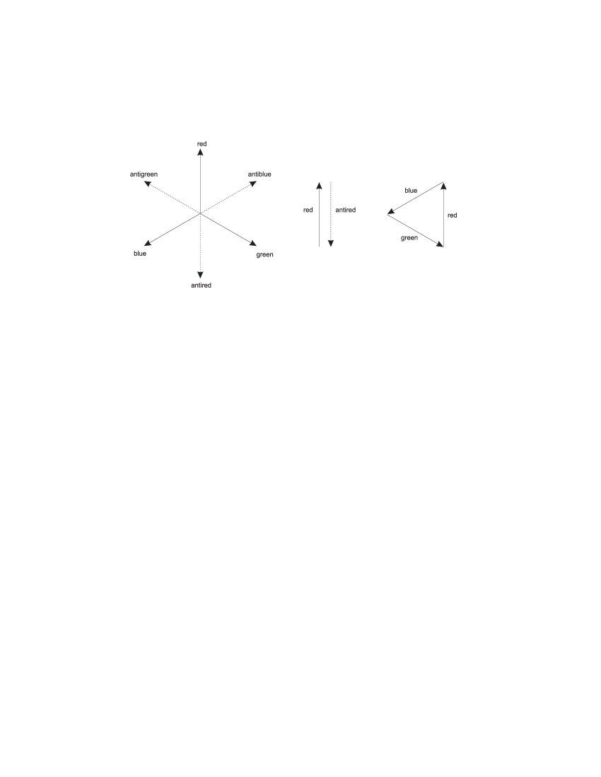
Figure 1.1: Graphical picture of the relation between the different colours and two examples of colourless, white states.

$$|\pi^{+}>=\left\{\begin{array}[]{c}\begin{tabular}[]{l}$u_{r}\overline{d}_{\overline{r}}>$\\ $u_{b}\overline{d}_{\overline{b}}>$\\ $u_{g}\overline{d}_{\overline{g}}>$\end{tabular}\end{array}\right.$$

A physical $\pi^{+}$ is equal to a quantum-mechanical mixture of these states.

1.3 Gluons

The force that binds quarks together is the strong interaction. It is mediated by its exchange particles, the gluons. The gluon is a spin-1 particle with no mass, and hence the strong interaction would have a long range would it not be screened. The effective range of the force is of the order of $10^{-15}$ m. The gluons carry both colour and anticolour. Since $3\times 3$ colour combinations exist, the gluons form two multiplets of states, an octet and a singlet. It is possible to construct all colour states from the octet and therefore there are eight different gluons. The ninth state is the totally symmetric state $R\overline{R}+B\overline{B}+G\overline{G}$, which is colourless, and therefore plays no role in the strong interaction.

Since gluons themselves carry colour they can interact with each other. This is the main difference between the strong and the electromagnetic interaction, since photons carry no electric charge. Gluons can be emitted and absorbed, created and annihilated, when a strong interaction is involved in a process.

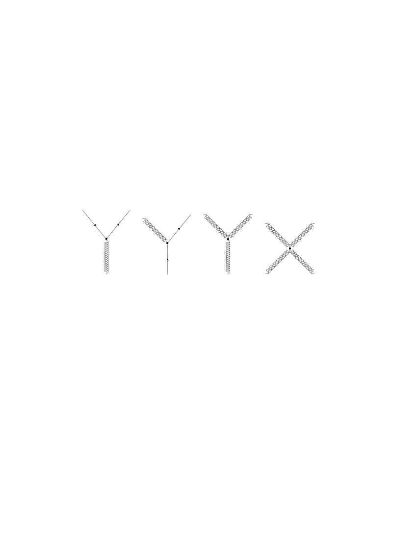
Figure 1.2: The fundamental interaction Feynman diagrams of the strong interaction. From left to right, splitting of a gluon into a quark-antiquark pair, emission of a gluon, and two gluon self-couplings.

Since quarks make up the proton and the neutron, gluons mediates the force that keep the proton and the neutron together. The strong nuclear force that makes the nucleons in a nucleus stick together, is in quark-gluon terms a leakage of the forces that keep the nucleons together, e.g. in the form of quark-antiquark pairs.

Since all quarks have the same possibility to carry a certain colour regardless of flavour, the strong interaction is flavour independent, i.e., all sorts of quarks have identical strong interactions.

One consequence of the properties of the strong interaction is that the strength of the strong force decreases when the quarks are close to each other. This property gives the quarks what is called asymptotic freedom at small inter-quark distances.

The strength of the strong interaction is described by the strong ”running” coupling constant $\alpha_{s}$. It has a direct dependence on the squared four-momentum transfer in the quark process:

$$\alpha_{s}(Q^{2})=\frac{12\pi}{(33-2N_{f})ln(Q^{2}/\Lambda^{2})}.$$ (1.1)

N_f is the number of quark flavours involved and $\Lambda$ is a scaling parameter, $\Lambda=0.2\pm 0.1$ GeV. From this expression, it is easy to see how $\alpha_{s}$ decreases with increasing momentum transfer. This is equivalent to decreasing $\alpha_{s}$ when the distance to a quark decreases. Hence, asymptotic freedom and colour confinement are implied by the expression for the strength of the interaction.

A more detailed account of the quantum field theory of the strong interaction (QCD) is given in the next chapter.

Chapter 2 Quantum chromodynamics

2.1 The concept of colour

A new quantum-mechanical gauge theory of quark interaction was born in the 1960s and 1970s. It was called QCD, in analogy with quantum electrodynamics (QED).

The basic idea with QCD is invariance against arbitrary rotations in colour space. Since the complex rotations of an arbitrary vector in three-dimensional space are described by unitary $3\times 3$ matrices of unit determinant, the symmetry group of the gauge transformation is $SU(3)$.

When the concept of colour was invented, the main reason was to make the quarks obey the Pauli principle, but at that time there was no evidence that there are exactly three colours. The experimental verification of the number of colours came in the beginning of the 1980s  [?]. The ratio of the production of hadrons from $e^{+}e^{-}$ collisions to that of muon pairs reveals an interesting fact. This is based on an assumption that the production of hadrons proceeds through creation of a quark-antiquark pair, which subsequently fragments into hadrons. In that case, the ratio of the cross-sections can be related to the sum over the square of the electromagnetical charges of all sorts of quarks that can be created. Defining $N_{c}$ as the number of colours, one gets

$$R=\frac{\sigma(e^{+}e^{-}\rightarrow hadrons)}{\sigma(e^{+}e^{-}\rightarrow\mu^{+}\mu^{-})}=N_{c}\sum_{i}e_{i}^{2}=\frac{11}{9}N_{c}$$ (2.1)

for i = $u,d,s,c,b$ quark types. The experiments yield $N_{c}=3$ without doubt  [?].

2.2 The QCD Lagrangian

The principle behind the QCD Lagrangian is the demand for invariance under local colour rotations, i.e., the gauge matrix $U$ changes from one point in space to another. In quantum electrodynamics (QED) the governing principle of gauge transformation is changes in the phase of the wave function, as described by the one-dimensional $U(1)$ symmetry group.

The approach in deriving the QCD Lagrangian is the same as in QED modified to fit the gauge invariance of the strong interaction. The fundamental QED Lagrangian is (see, e.g.  [?]):

$$L_{QED}=i\overline{\psi}\gamma^{\mu}(\partial_{\mu}+ieA_{\mu})\psi-m\overline{\psi}\psi-\frac{1}{4}F^{\mu\nu}F_{\mu\nu},$$ (2.2)

where $F^{\mu\nu}=\partial_{\mu}A_{\nu}-\partial{{}_{\nu}}A_{\mu}$ is the electromagnetic field strength tensor, and $A_{\mu}$ is the electromagnetic vector field.

Due to the colour property, the wave function of a quark has three components in colour space, $\psi=(\psi_{r},\psi_{g},\psi_{b})$. A colour gauge transformation, $\psi\rightarrow U\psi$, is described by a unitary $3\times 3$ matrix $U$ with $det(U)=1$. $U$ can be written as the imaginary exponential of a Hermitian matrix $L$, $U=exp(iL)$, where $L^{*}=L$ and $tr(L)=0$. All traceless Hermitian $3\times 3$ matrices can be expressed as linear combinations of the eight $\lambda$-matrices  [?]

$$L=\frac{1}{2}\sum_{a=1}^{8}\theta_{a}\lambda_{a}.$$ (2.3)

Here

$$\left[\lambda_{a},\lambda_{b}\right]=2if_{abc}\lambda_{c}\hskip 14.22636pt\mbox{and}\hskip 14.22636pt\left[\lambda_{a},\lambda_{b}\right]_{+}=\frac{4}{3}\delta_{ab}+2d_{abc}\lambda_{c}.$$ (2.4)

These so-called Gell-Mann matrices, or $\frac{1}{2}\lambda_{a}$ to be more exact, are the eight generators of the Lie group $SU(3)$, and $f_{abc}$ and $d_{abc}$ are the antisymmetric and symmetric structure constants. To make the rotation $U$ space-dependent the real parameter $\theta_{a}$ must vary in space, $\theta_{a}=\theta_{a}(x)$. This leads to

$$U(x)=exp\left[\frac{1}{2}\sum_{a=1}^{8}\theta_{a}(x)\lambda_{a}\right]$$ (2.5)

Thus $\psi\rightarrow U(x)\psi$ gives

$$\partial_{\mu}[U(x)\psi]=U\partial_{\mu}\psi+(\partial_{\mu}U)\psi=U[\partial_{\mu}\psi+U^{*}(\partial_{\mu}U)\psi].$$ (2.6)

Since $U\partial_{\mu}\psi$ should be present in the right-hand side one has to introduce a colour potential, the analogue to the electromagnetic potential $A_{\mu}$ in QED. That potential is called $\widehat{A}_{\mu}$; a $3\times 3$ Hermitian matrix. This $\widehat{A}_{\mu}$ can be represented as a linear combination of Gell-Mann matrices:

$$\widehat{A}_{\mu}(x)=\frac{1}{2}\sum_{a=1}^{8}A_{\mu}^{a}(x)\lambda_{a}.$$ (2.7)

The field $\widehat{A}_{\mu}(x)$ is called a Yang-Mills field  [?], and if $\widehat{A}_{\mu}(x)$ changes during a colour rotation according to

$$\widehat{A}_{\mu}\rightarrow U^{*}\widehat{A}_{\mu}U-i\frac{1}{g}U^{*}(\partial_{\mu}U),$$ (2.8)

the derivative $(\partial_{\mu}-ig\widehat{A}_{\mu})$ will be invariant under such gauge transformations. Here $g$ is the so-called strength factor of the strong field. Since the basic relation is the Dirac equation one can choose a potential that leaves the derivative invariant under such a gauge transformation making the whole equation invariant. The replacement defines a covariant derivative, $D_{\mu}=\partial_{\mu}\rightarrow$ $(\partial_{\mu}-ig\widehat{A}_{\mu})$.

The next step is to add a kinetic term to the Lagrangian, and a first guess is a QED-like term, $-\frac{1}{4}F^{\mu\nu}F_{\mu\nu}$. It turns out that one has to modify the definition of the field strength tensor $F_{\mu\nu}$ in order to keep the theory gauge invariant. Since no interactions take place between two photons, QED is an abelian theory and the generators of the $U(1)$ group commute. QCD, on the other hand, is a non-abelian $SU(3)$ local gauge theory. The generators are non-commutative, due to the fact that interactions take place between the gluons. The field strength tensor therefore changes to

$$F_{\mu\nu}^{a}=\partial_{\mu}A_{\nu}^{a}-\partial_{\nu}A_{\mu}^{a}+gf_{abc}A_{\mu}^{b}A_{\nu}^{c},$$ (2.9)

and this definition makes it form invariant under a local colour gauge transformation, $F_{\mu\nu}\rightarrow U^{*}F_{\mu\nu}U$.

The complete QCD Lagrangian is then

$$L_{QCD}=i\overline{\psi}\gamma^{\mu}(\partial_{\mu}-ig\widehat{A}_{\mu})\psi-m\overline{\psi}\psi-\frac{1}{4}F_{\mu\nu}^{a}F_{a}^{\mu\nu}.$$ (2.10)

Notice the resemblance with the QED Lagrangian, eq. (2.2). All the difference lies in the self-interaction term in the definition of $F_{\mu\nu}$ and in the exchange of $+ieA_{\mu}\rightarrow-ig\widehat{A}_{\mu}$.

Chapter 3 The confinement of coloured particles

3.1 The confinement mechanism

The non-observation of single quarks led the physicists to postulate that no particle can exist in a coloured state, and as a consequence, to establish the concept of quark confinement.

QCD has complex field equations that make it unsuitable for ”exact” calculations. This leads to extensive use of perturbative methods. These are, on the other hand, valid only in certain regimes of the perturbative expansion parameter. In QCD, this parameter is the strong coupling constant, $\alpha_{s}$. It gets small when the four-momentum transfer is large or, equivalently, the distance involved is small as illustrated by eq. (1.1). That makes perturbative QCD valid only in processes that have these characteristics. This is unfortunate because the distance when $\alpha_{s}$ gets too large for a perturbative expansion, is about the same as the dimensions of a hadron. Therefore, the confinement mechanism cannot be derived directly from the QCD Lagrangian, and confinement cannot even be proven. Instead, one has to use ”QCD-inspired”, phenomenological models to describe confinement.

3.2 The QCD vacuum

The expression for the strong coupling constant eq. (1.1) is derived from the full gluon propagator, $D(q^{2})$ where $q^{2}=-Q^{2}$. This propagator is essentially the boson propagator, but it has been modified due to vacuum polarization.

It is possible, to reach the same quantative conclusion involving the QCD vacuum, which follows a line of reasoning by Gottfried and Weisskopf  [?].

Let us consider the empty vacuum, i.e., one where there are no gluons. To this vacuum, add a pair of gluons of opposite colour charges and spincomponents, and with an average separation $r$. The energy for this pair is

$$E(r)=\frac{A}{4\pi r}-\frac{C\alpha_{s}}{4\pi r}\hskip 21.33955pt\mbox{for}\hskip 21.33955ptr\lesssim r_{0},$$ (3.1)

where A and C are constants. The first term is the kinetic energy and the second one is the potential energy. $r_{0}$ is the distance where $\alpha_{s}$ gets ”large”. For $r\ll r_{0}$, $\alpha_{s}$ is small and $E(r)$ positive, but near $r_{0}$, $E(r)<0$! When $r>r_{0}$ the expression is no longer valid, but it should suffice to assume that $E(r)$ increases with $r$.

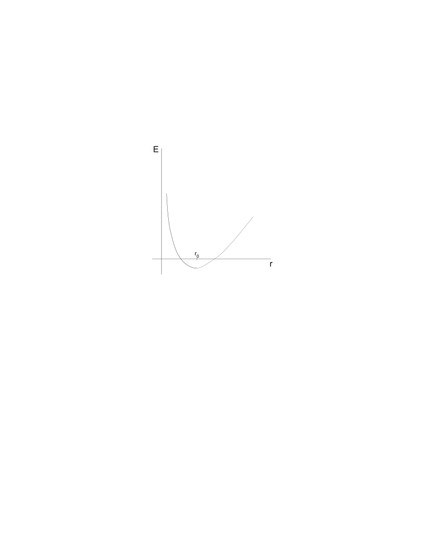
Figure 3.1: The energy $E$ of the gluon pair versus distance $r.$

If this picture is correct, it seems to be energetically favourable to create a gluon pair with opposite spins and colours out of the ”empty” vacuum, to take advantage of the negative energy when $r\sim r_{0}$.

The true vacuum can now be described as follows. The ”empty” vacuum is unstable. There exists a state of lower energy that consists of cells, each containing a gluon pair in a colour- and spin-singlet state. The size of these cells is of order $r_{0}$.

This give one a crude description of how a colour-neutral assembly of quarks is immersed into the gluon vacuum. The gluonic cells will be displaced by the quarks, and therefore the quarks will find themselves in a gluon-free ”bubble” or ”bag”. A state with quarks and gluons in the same bag has a higher energy, and therefore the quarks ”push away” the gluon field. The size of this ”bag” is of the order of 1 fm. Since the true vacuum has an energy density lower than the ”empty” vacuum, the energy density in the bag must be positive. Actually, it is proportional to the bag volume, $V$:

$$E_{B}=BV.$$ (3.2)

$B$ is called the bag constant and has the dimension of (energy)⁴ provided that one sets $c=\hbar=1$ so that distances are counted in 1/eV. The region outside the bag exerts a pressure on the bag which is counteracted by the kinetic energy of the quarks. It can be shown  [?] that this picture describes the observed structure, size and low-lying spectra of hadrons reasonably well if $B^{1/4}\approx 150$ MeV. The pressure on the bag then amounts to $\sim 10^{23}$ atm.

Now one can compare the field of two opposite electric charges with the field of two opposite colour charges at a separation larger than $r_{0}$. In the electromagnetic case the field lines spread when the separation grows.

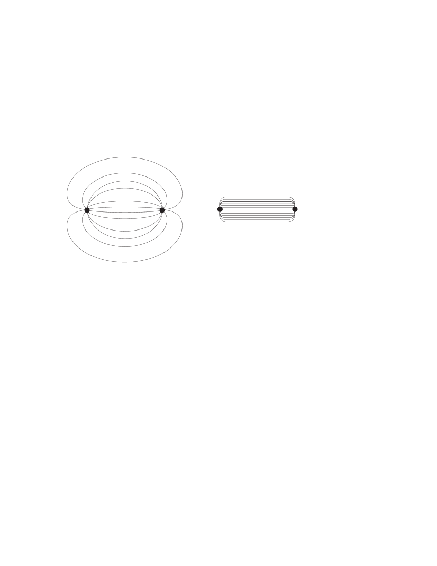
Figure 3.2: Phenomelogical picture comparing the nature of the strong force with the electromagnetical force.

The number of electric field lines crossing a unit area decreases like $r^{-2}$. In the colour case, the pressure of the true vacuum compresses the field lines into a tube of diameter $r_{0}$. When $r\gg r_{0}$ the number of field lines per unit area within this tube remains constant, leading to a constant force, i.e., a linear potential:

$$\phi(r)=ar\hskip 21.33955pt\mbox{for}\hskip 21.33955ptr\gg r_{0}.$$ (3.3)

The experimental value of the constant $a$ is $a\sim 0.6$ GeV/fm.

In conclusion, there is a constant force acting on a quark if one tries to remove it from a hadron to distances larger than $r_{0}$. If one would like to remove it completely one would need an infinite amount of energy. However, long before that, the colour field would ”break up” into new quark-antiquark pairs.

3.3 Bag models

Since the potential in QCD grows indefinitely with distance, coloured particles are confined to each other. The so-called bag models have been invented to take this into account, because the exact QCD formalism is virtually impossible to solve for bound hadronic states (just like QED for atoms). In these models, quarks are confined to a certain hadronic volume $V$. The Dirac equation for the quarks becomes

$$i\gamma^{\mu}\partial_{\mu}\psi-m\psi=0$$ inside (3.4)

$$\psi=0 \mbox{{\it outside}}.$$

Then, the quark current through the surface is zero. This makes the boundary condition read

$$n_{\mu}j^{\mu}=n_{\mu}(\overline{\psi}\gamma^{\mu}\psi)=0.$$ (3.5)

This bag model was proposed by Bogolioubov in 1967  [?].

3.4 The MIT bag model

In the mid 1970s a group of physicists at the Massachusetts Institute of Technology (MIT) showed that Bogolioubov’s bag model leads to energy-momentum conservation violation at the bag surface, unless the internal pressure from the interior of the bag is balanced by an external pressure. This led to a modified model, the MIT bag model  [?,?,?], where the true vacuum inside the bag is partially destroyed by quarks carrying colour. This mixture of quarks and true vacuum made it possible to treat the physics of the interior of the bag by perturbative QCD, a so-called perturbative vacuum inside the bag. This change in the bag model leads to a new boundary condition. The requirement of pressure balance at the surface is written as

$$-\frac{1}{2}n^{\mu}\partial_{\mu}(\sum_{i}\overline{\psi_{i}}\psi_{i})|_{S}=B,$$ (3.6)

where $B$ is the bag constant, and the sum runs over all quarks contained in the bag. For a spherical bag this condition is equivalent to the requirement that the total energy contained in the bag volume should be at a minimum with respect to the bag radius $R$. Hence $\frac{\partial M}{\partial R}=0$, where

$$M(R)=\frac{(\sum_{i}x_{i})}{R}+\frac{4\pi}{3}BR^{3},$$ (3.7)

$x_{i}=\omega_{i}R$, and $\omega_{i}$ are the eigen-frequencies of the solutions to the Dirac equation. The equilibrium radius is obviously

$$R_{0}=\left(\frac{\sum_{i}x_{i}}{4\pi B}\right)^{\frac{1}{4}}.$$ (3.8)

It is possible to include real gluons in the bag even without quarks. Such states, ”glueballs” have not been found, although signals of hybrid glueball/quark states are sometimes reported. The appropriate boundary condition for the colour field is obtained from the requirement that the colour-electric field should not be able to penetrate outside the bag. The situation is analogous to the boundary condition in classical electrodynamics for a medium with $\varepsilon=0$ and $\mu=\infty$. By virtue of Gauss’ theorem an integration of the colour-electric field yields the result that the total colour charge contained in the bag volume vanishes.

There are several flaws in the MIT bag model, for instance,

• that the mass of the pion comes out too large in all versions of the model

• that the boundary condition is not chirally invariant, or equivalently, the MIT bag model violates PCAC, Partially Conserved Axial Vector Current.

Several attempts have been made to overcome these difficulties. In the chiral bag models a pion field has been added as an independent degree of freedom  [?,?]. In the cloudy-bag model  [?,?], or in the Tel Aviv model  [?], the pion cloud is allowed to penetrate into the bag. In these models, the main goal has been to make the model chirally invariant at the surface.

One of the models, the soliton bag model, where the large mass of a quark outside the bag is generated by the coupling to a scalar field, is very well suited for the description of the dynamical properties of the bag, such as vibrations of the bag surface. This model could be useful in the study of giant QGP bags.

It is important to remember that all the bag models are only attempts to construct a model that explains the behaviour of the particles as measured in experiments. As of this date, the mechanism of confinement is well established experimentally, but since perturbative QCD cannot be used in this region the theoretical understanding of confinement is incomplete.

Chapter 4 The transition to a quark-gluon plasma

4.1 Hadrons as systems of quarks

Ordinary matter is made out of leptons and hadrons. Hadrons are strongly interacting particles consisting of quarks. We know from statistical physics and thermodynamics that macroscopic systems of ordinary matter exhibit changes in phases when the environment changes in a specific way. Why should not nucleons, built of quarks, exhibit some change in phase when the environment changes?

It is experimentally justified to describe collisions of nuclei, i.e., systems of hadrons, in thermodynamic terms. The predicted temperatures in the collisions are in accord with experimental results. This temperature can be estimated from the energy distribution of the emitted fragments. The only discrepancy appears when the impact energy gets very high, the temperature does not increase as fast as the model suggests. The temperature seems to approach some kind of plateau when the collision energy grows. The temperature of boiling water does not change during the phase transition when the water enters its vapour phase. Would colliding nuclei approach some kind of analogue phase change? It turns out that the levelling-off of the temperature is due to the fact that higher-mass hadrons are created in the collision. The energy in the collision is high enough to convert into mass and create heavier hadrons than protons and neutrons.

It is possible to look at such a creation of hadrons as a kind of phase transition. It has a latent heat just as the liquid-vapour transition in water. The temperature in the collision remains the same until the most massive hadron have been created. Then the temperature starts to increase again. Hagedorn has suggested that there exists such a limit, and the limiting temperature should be about $1.5\cdot 10^{12}$ K  [?]. This is not so far away from current accelerator experiments.

4.2 From hadronic matter to QGP

The ultimate phase transition would be the transition from hadronic matter to a quark-gluon plasma. In the plasma phase the nucleons and the higher mass hadrons created in the collision lose their identity as individual particles.

It is important to remember the difference between the bonding of an electron to a nucleus and the bonding between quarks in a nucleon. It is possible with a finite investment of energy to separate an electron from a nucleus, and turn a gas into a plasma where all electrons move freely. But in a nucleon, one would need an infinite amount of energy to separate a quark from its environment.

There are two ways to create a plasma in a gas of atoms. One is to heat the gas until the collisions between the atoms are violent enough to rip away all electrons. Another is to compress the gas, driving the atoms into close contact and make their electronic shells overlap. Under these conditions the electrons are deconfined and can move freely from one atom to the other.

As explained earlier, the quark interaction is negligible at short distances (asymptotic freedom). On the other hand, when the distance increases the interaction also increases (confinement). These characteristics rule out the first way (heating) to create a quark-gluon plasma, but not the second one (compression). Hence, when making a quark-gluon plasma one does not need to set the quarks free, only to push them into the same bag. It should be added that it is at least theoretically possible to create a plasma by heating, although the phase transition is not obtained by quark deconfinement but by a more subtle mechanism  [?].

4.3 The QCD phase transition

At low energies, the QCD vacuum is characterized by nonvanishing expectation values of vacuum condensates, the quark condensate having $<\overline{\psi}\psi>\approx(235$ MeV$)^{3}$ and the gluon condensate having $<\alpha_{s}G_{\mu\nu}G^{\mu\nu}>\approx(500$ MeV$)^{4}$. The quark condensate describes the density of quark-antiquark pairs found in the QCD vacuum and is the expression of chiral symmetry breaking. The gluon condensate measures the density of gluon pairs in the QCD vacuum and is a manifestation of the breaking of scale invariance of QCD by quantum effects.

Broken symmetries in nature are often restored through phase transformations at high temperatures. Some examples are ferromagnetism, superconductivity and the transformation from solid to liquid. In the quark-gluon plasma case, the phase transition from hadronic matter to quark-gluon plasma would restore the broken chiral symmetry. Nuclear matter at very high temperature would exhibit neither confinement nor chiral symmetry breaking.

It is known from quantum field theory that chiral symmetry is broken if the particles involved have non-zero mass. But in the QCD vacuum, a non-zero value of the quark-antiquark condensate expectation value $<\overline{\psi}\psi>$ has the same effect. The density of spin-0 quark-antiquark paris has the chiral decomposition $q\overline{q}=\overline{q}_{L}q_{R}+q_{L}\overline{q}_{R}$, where subscripts $R$ (”right-handed”) and $L$ (”left-handed”) denote states with spin parallel and antiparallel to the direction of motion. Hence the broken vacuum state contains pairs of quarks of opposite chirality. If a left-handed quark annihilates a left-handed antiquark, then the process is perceived as a change of chirality of the free quark, exactly the same effect as a non-vanishing quark mass. In reality though, the light quarks have mass and the chirality of a light quark is not conserved, even if the quark condensate vanishes.

When the temperature increases the interactions occur at shorter distances, mainly by the weak coupling because the long range strong interaction gets dynamically screened. Finite temperature perturbation theory shows that the strong coupling constant $\alpha_{s}$ falls logarithmically with increasing temperature  [?,?]. The result that the quark-condensate parameter vanishes at high temperature, makes it likely that the transition between the low-temperature and the high-temperature manifestations of QCD shows a discontinuity, i.e., a phase transition. The order of this transition is believed to depend on the number of light, quark flavours. Two massless flavours would generate a second-order transition  [?,?] while three massless flavours give a first-order transition.

Numerical simulations indicate that the transition temperature lies in the range $150\pm 10$ MeV  [?].

Chapter 5 The properties of a QGP

5.1 Equation of state

Considering the energy scale in the hot QGP, i.e., $\sim 200$ MeV, the approximation that the plasma only contains $u$ and $d$ quarks which are massless should be quite reasonable. With this approximation and the assumption that one can neglect all quark interactions inside the plasma, one can derive the equation of state  [?].

First, one needs to count the degrees of freedom for the constituents:

$$\mbox{Gluons:}\hskip 14.22636ptN_{g}=2(spin)\times 8(colour)=16$$ (5.1)

$$\mbox{Quarks:}\hskip 14.22636ptN_{q}=2(spin)\times 2(flavour)\times 3(colour)=12.$$ (5.2)

The energy density residing in each degree of freedom is calculated separately for the quarks and the gluons. The gluons form, without the interactions, an ideal relativistic Bose gas of temperature $T$ which gives the energy density

$$E_{g}=\int\frac{d^{3}p}{(2\pi)^{3}}\frac{p}{(e^{\beta p}-1)}=\frac{\pi^{2}T^{4}}{30},$$ (5.3)

where $\beta=1/T$. For the quarks and the antiquarks one has to introduce a chemical potential $\mu$ because, in general, there will be a slight surplus of quarks over antiquarks in the QGP created from normal atomic nuclei (heavy ions). At zero temperature, $\mu$ is the energy needed to add another quark to the plasma. Since no antiquarks are present at $T=0$ the energy necessary to add an antiquark is zero. This does not imply that $\mu=0$, because the additional antiquark may annihilate a quark and release the energy $\mu$, assuming that the quark lies at the surface of the Fermi sea. The chemical potential of the antiquarks must therefore be chosen as $-\mu$.

The energy density for the quarks, treated as a relativistic Fermi gas, cannot be calculated analytically if $\mu,T\neq 0$. However, the energy density for a quark and an antiquark is

$$E_{q} = \int\frac{d^{3}p}{(2\pi)^{3}}\frac{p}{[e^{\beta(p-\mu)}+1]},$$ (5.4)

$$E_{\overline{q}} = \int\frac{d^{3}p}{(2\pi)^{3}}\frac{p}{[e^{\beta(p+\mu)}+1]},$$ (5.5)

$$E_{q}+E_{\overline{q}} = \int\frac{d^{3}p}{(2\pi)^{3}}\left\{\frac{p}{[e^{\beta(p-\mu)}+1]}+\frac{p}{[e^{\beta(p+\mu)}+1]}\right\}$$

$$= \frac{7\pi^{2}}{120}T^{4}+\frac{\mu^{2}}{4}T^{2}+\frac{\mu^{4}}{8\pi^{2}}.$$

Considering baryon-number symmetric quark-gluon matter, i.e., $\mu=0$, and multiplying with the respective degrees of freedom, the energy density becomes

$$E=16E_{g}+12(E_{q}+E_{\overline{q}})=\frac{37\pi^{2}}{30}T^{4}=\left(\frac{T}{160\mbox{ MeV}}\right)^{4}\left[\mbox{GeV/fm}^{3}\right].$$ (5.7)

The expressions above use $k_{B}=c=\hbar=1$, giving $T$ the dimension of energy, and length the dimension of (energy^-1). The energy density inside a nucleon is four times the MIT bag constant, $E_{N}=4B\approx 300-500$ MeV/fm³, which together with a transition temperature of $\sim 150$ MeV gives an energy density of the QGP of $\sim 1-1.5$ GeV/fm³. From this one can see that one needs at least a factor of two higher energy densities than inside a nucleon in order to make a QGP.

But what if $\mu\neq 0$? One can still use eq. (5.7) but $\mu$ must now be computed, i.e., one has to know its relation to the baryonic density $n_{B}$. This density is one third of the density difference between the quarks and the antiquarks multiplied with the degrees of freedom:

$$n_{q}=\int\frac{dp}{e^{\beta(p-\mu)}+1},$$ (5.8)

$$n_{\overline{q}}=\int\frac{dp}{e^{\beta(p+\mu)}+1},$$ (5.9)

$$n_{q}-n_{\overline{q}}=\frac{\mu}{6}T^{2}+\frac{\mu^{3}}{6\pi^{2}}$$

$$\Longrightarrow n_{B}=4(n_{q}-n_{\overline{q}})=\frac{2\mu}{3}T^{2}+\frac{2\mu^{3}}{3\pi^{2}}.$$ (5.10)

Hence $n_{B}=\frac{4}{3}\frac{\partial E}{\partial\mu}$ where $E=E_{q}+E_{\bar{q}}$ is taken from eq. (5.1). The pressure and entropy of the plasma are given by

$$p=\frac{1}{3}E,$$ (5.11)

$$s=\frac{1}{3}\frac{\partial E}{\partial T}.$$ (5.12)

Under what conditions should the bag containing the plasma be stable? A fair assumption would be that the external vacuum pressure, characterized by the bag constant $B$, should not exceed the internal pressure, i.e., $p=\frac{E}{3}\geq B$. The critical temperature $T_{c}$ and the critical chemical potential $\mu_{c}$ can be calculated using the eqs. (5.7) and (5.11) evaluated at the critical pressure $p_{c}=B$:

$$B=p_{c}=T_{c}^{4}\left[\frac{37\pi^{2}}{90}+\left(\frac{\mu_{c}}{T_{c}}\right)^{2}+\frac{1}{2\pi^{2}}\left(\frac{\mu_{c}}{T_{c}}\right)^{4}\right].$$ (5.13)

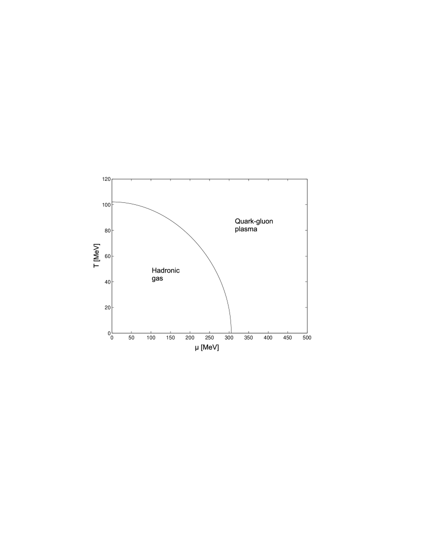
Figure 5.1: A typical result from eq. (5.13), showing the relation between the critical values of the temperature T and the chemical potential $\mu$. The bag pressure $B^{1/4}=145$ MeV was used.

Considering also perturbative interactions in the QGP, a second-order thermal perturbative calculation gives  [?]

$$E=\frac{8\pi^{2}}{15}T^{4}\left(1-\frac{15\alpha_{s}}{4\pi}\right)+3\sum_{f}\left[\frac{7}{60}\pi^{2}T^{4}\left(1-\frac{50\alpha_{s}}{21\pi}\right)+\right.$$ (5.14)

$$\left.+\left(\frac{1}{2}T^{2}\mu_{f}^{2}+\frac{1}{4\pi^{2}}\mu_{f}^{4}\right)\left(1-\frac{2\alpha_{s}}{\pi}\right)\right]+B,$$

where $f$ is the quark flavour (neglecting quark masses). This formula includes also the effect of strange quarks ($s\bar{s}$ pairs), provided they can be treated as massless. However, it does not include short-range spin effects in QCD, so-called colour-magnetic forces. These tend to favour quarks to form spin-0 pairs (”diquarks”). For a review of such effects, see  [?]. Would such effects be important, the QGP should rather be treated as a boson gas, or a boson-fermion mixture. Such non-perturbative phenomena cannot be rigorously treated within QCD.

5.2 The formation of a QGP - experiments

There are only two known situations where a QGP object could form

• In a very hot and dense astrophysical environment, for instance, in the early Universe or in the interior of a heavy neutron star or a collapsing star, as will be discussed in a separate chapter

• In a high-energy heavy-ion collision taking place in an accelerator or due to cosmic rays.

A central high-energy collision between heavy nuclei, resulting in a compression of nuclear matter, is the most promising process fir creating a QGP in a laboratory environment. There are presently several such experiments running at the SPS collider at CERN and the AGS collider at Brookhaven. Two more colliders are under construction, LHC at CERN and RHIC at Brookhaven.

Facility Location Starting date Energy/nucleon

AGS Brookhaven, USA 1986 4.84 GeV

SPS CERN, Switzerland 1986 17.2 GeV

RHIC Brookhaven, USA 1999 200 GeV

LHC CERN, Switzerland $$\sim$$ 2005 5.4 TeV

There are three distinguishable processes in models of ultra-relativistic heavy-ion collisions and QGP formation. The first is the collision of the two nuclei and the formation of the thermalized QGP. Several models have been developed to describe this dynamical process, e.g. the partonic cascade model  [?] and the QCD string-breaking model based on the Lund string model  [?]. An overview is given in  [?]. The second process involves the (relativistic) hydrodynamic behaviour of the plasma. The third process is when the plasma has cooled to the critical temperature, $T_{c}\approx 150-200$ MeV, and starts to hadronize.

Several detailed calculations have been presented  [?,?,?] in support of the view that a thermalized QGP will be produced in the planned experiments at RHIC and LHC.

5.3 The decay of a QGP

The decay of a QGP is believed to take place along one of two possible decay channels. It may expand until the density drops below the threshold of stability for quark matter, or it may hadronize through emission of particles, mainly pions, from the surface of the confining bag.

It can be shown by a fairly simple reasoning  [?] that pion evaporation cannot be the dominant process in the decay of the plasma. There are three possible processes that can create pions on the surface of a QGP bag:

• A quark loses kinetic energy while bouncing off the surface from inside.

• An antiquark loses kinetic energy while bouncing off the surface.

• A quark and an antiquark annihilate at the surface, emitting a pion.

The energy emission through these three processes is  [?]

$$\frac{d^{3}E}{dtd^{2}x}\approx 0.02\frac{T^{6}}{f_{\pi}^{2}}$$ (5.15)

where $f_{\pi}$ is the decay constant of the pion and $x$ is a spatial dimension. The cooling by pion emission increases with temperature, but integrating eq. (5.15), the pion radiation falls below the thermal emission rate up to temperatures of $300$ MeV. This leads to the conclusion that cooling by pion radiation is probably not a major channel of energy loss.

This supports the other alternative, i.e., that the plasma will expand until it reaches the critical temperature $T_{c}$ and then convert into a hadronic gas, while maintaining thermal and chemical equilibrium. A similar approach  [?] is that the partonic reactions inside the bag change the parton density locally so that a hadron can be formed. Hence, the reactions split the bag into smaller regions, where the hadrons form due to local density fluctuations.

The decay due to expansion and cooling hence seems to be the dominant mechanism, and the lifetime of a QGP should be a few times $10^{-23}$ s.

Chapter 6 Signatures of a QGP

In order to detect a QGP one needs some clear experimental signatures of its formation and/or decay. Many such signatures have been suggested in the literature, and some of them are reviewed here. Searching for a QGP formation is an event-by-event search where the events detected by the detector can be connected to some signature of a QGP. If the critical energy density is reached, several types of reactions are possible, not only QGP formation. In experiments one tries to select events with central collisions, i.e., with a small impact parameter, where high mass densities are most likely to occur. This can be done by focusing on events with, e.g. high multiplicities, many nuclear fragments or protons or a high symmetry around the beam axis.

6.1 Kinematic probes of the equation of state

Such probes are based on the energy density, pressure and entropy of superdense hadronic matter as a function of the temperature and chemical potential. One looks for a rapid rise in the effective degrees of freedom, as expressed by the ratios $\frac{E}{T^{4}}$ or $\frac{s}{T^{3}}$ over a small temperature range ($s$ being the entropy). If a first-order phase transition takes place, these quantities exhibit a discontinuity or a step-like rise  [?].

It is impossible to directly measure temperature and energy density. Instead, one measures the average transverse momentum, $<p_{T}>$, and the rapidity distribution of the produced hadrons, $\frac{dN}{dy}$. These quantities can be theoretically related to the variables $T,\,s$ and $E$. If a rapid change occurs in the effective number of degrees of freedom, which would happen if a QGP was formed, one would see an s-shaped curve in a plot of $<p_{T}>$ versus $\frac{dN}{dy}$. This plot serves as a phenomenological phase diagram, and expresses the simple fact that a QGP decay is expected to give many hadrons, and that they would get high $p_{T}$ values due to the high temperature.

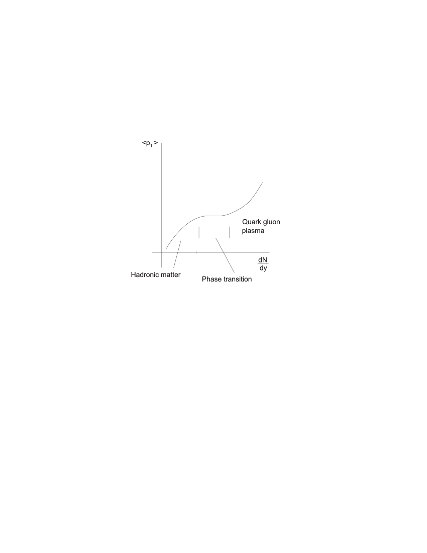
Figure 6.1: A schematic plot of the expected behaviour of the mean transverse momentum versus the density of produced particles in rapidity space.

There are other methods built on similar ideas, reviewed in  [?].

6.2 Electromagnetic probes

The clearest signal of the QGP is probably an excess of produced lepton paris and photons. They probe the earliest and hottest phase of the evolution of the QGP fireball without being affected by final-state interactions. The drawback is that these signals are supposed to be rather weak and cluttered with signals from hadronic processes.

Lepton pairs have for long been considered clear probes of the QGP. Thermal di-leptons are produced when a quark and an antiquark annihilate in a QGP. However, this so-called Drell-Yan lepton-pair production occurs also in normal hadron collisions. Recent calculations  [?,?,?,?] show that lepton pairs from the equilibrating QGP may dominate over Drell-Yan production where invariant lepton masses are in the range $1-10$ GeV. If lepton pairs can be measured above the expected Drell-Yan background from nucleon-nucleon collisions up to several GeV of invariant mass, the early thermal evolution of the QGP phase can be traced in a rather model independent way  [?].

Also photons from the QGP compete with the background of several hadronic reactions. The hadronic radiation spectrum is not concentrated in a single narrow resonance. In fact, a hadron gas and a QGP in the vicinity of the transition temperature $T_{c}$ emit photon spectra of roughly equal intensity and similar spectral shape  [?]. If the QGP temperature lies clearly above $T_{c}$, a signal of photons from the QGP phase would be visible  [?,?,?].

6.3 Strangeness enhancement, related probes

The most commonly proposed signatures of restored chiral symmetry in dense baryon-rich hadronic matter are enhancements in strangeness and antibaryon production. The production of hadrons containing strange quarks is normally suppressed in nuclear reactions  [?], because $s$ quarks do not exist in the original heavy ions. When a QGP is formed, the production of hadrons containing $s$ quarks is expected to be saturated thanks to the production of $s\bar{s}$ pairs  [?]. The yield of strange baryons and antibaryons is therefore predicted to be strongly enhanced in the presence of a QGP  [?,?].

There has been many observations of elevated strange-particle production in nuclear collisions. However, such an enhancement alone cannot prove the presence of a QGP. Strange particles can be copiously produced in hadronic reactions, and several calculations have been presented  [?,?]. Nevertheless, the enhancement of $\Lambda$ production over a wide rapidity range, observed in heavy-ion collisions at 200 GeV/nucleon does not seem to be explained by these models. Unfortunately, it would be premature to conclude that a QGP has been formed. The QGP calculations use the assumption that final-state interactions in the decay of the QGP do not modify the hadron yield, while there are strong reasons to believe that the strangeness-carrying hadrons interact strongly. Therefore final-state interactions could very well erase all traces of the plasma phase.

A strangeness abundance can still be a useful trigger for verifying other signals of a QGP.

As stated earlier, a phase transition from hadronic matter to QGP would restore the broken chiral symmetry, i.e., make the quarks behave as if massless, or very light. This symmetry breaks down again when the plasma decays into normal hadrons resulting in the formation of so-called disoriented chiral condensates, DCC  [?]. The DCC would later decay into neutral and charged pions, favouring a neutral-to-charge ratio different from the value of 1/2 from isospin symmetry. Such events that virtually violate isospin symmetry have been observed, namely the so-called Centauro events from cosmic rays interacting in the atmosphere  [?].

6.4 Hard QCD probes of deconfinement

It is commonly believed that a $c\bar{c}$ pair produced by fusion of two gluons cannot bind inside the QGP. Therefore, $J/\psi$ production is suppressed in the collision of two nuclei forming a QGP compared to a normal hadronic process. This assumption is based on the fact that a bound state cannot exist when the colour screening length $\lambda_{D}\approx\frac{1}{gT}$ is less than the bound-state radius $<r_{J/\psi}^{2}>^{1/2}$  [?]. Computer simulations have shown that this seems to happen slightly above the transition temperature $T_{c}$, say at $T\sim 1.2$ $T_{c}$. The formation of the $c\bar{c}$ system takes a time of about 1 fm/c, and therefore it could require a rather long QGP lifetime before the suppression becomes effective. The details of modeling $J/\psi$ suppression near $T_{c}$ are quite complicated and the phenomenon has been extensively studied by several authors  [?,?,?,?,?,?,?,?,?,?,?]. There has been experimental observations of $J/\psi$ suppression in Pb-Pb collisions by the NA38 experiment at the CERN-SPS  [?]. There are, however, other hadronic mechanisms that could explain the results equally well  [?]. Quarkonium suppression is nevertheless believed to be the most promising signal so far of the formation of a QGP.

Hard partons, i.e., quarks or gluons with very high energies, are believed to be formed at the early phase transition. If such a parton travels through a deconfined medium, it finds much harder gluons to interact with than it would in a confined medium where the gluons are constrained by the hadronic parton distribution  [?]. The mechanisms in this case are similar to those responsible for the electromagnetic energy loss of a fast charged particle in matter. Energy may be lost either by excitation of the penetrated media or by radiation. Fast partons lose much more energy per unit length in a QGP than in hadronic matter. Hence the energy loss could tell whether or not the parton has travelled through a QGP. On the other hand, the average transverse momentum, $<p_{T}>$, of produced hadrons is supposed to be enhanced from a QGP, due to the high temperature. A suppression of hard partons can therefore be difficult to disentangle from the rise in $<p_{T}>$.

6.5 Signatures - a summary

It is obvious that a QGP can only be detected by the use of a combination of signals from different stages of the high-temperature phase of QCD. The signals discussed here all have normal hadronic counterparts. However, the overall signals of a QGP would presumably not be simultaneously duplicated by normal hadronic reactions.

The QGP has yet to be uniquely observed or identified, but there are data that appear as rather promising. One such example is the detection of an enhancement of strange particles made at both the AGS  [?] and the SPS  [?,?,?,?,?]. The enhancement in the $\Lambda$ yield measured over a large rapidity interval is difficult to describe from purely hadronic interactions. An equilibrated QGP with strangeness neutrality and large strangeness saturation, which hadronizes and decays instantaneously, fits the SPS data  [?,?,?], but further experimental information is necessary to rule out other explanations. The current (1996), experimental situation is discussed in  [?].

Chapter 7 Astrophysical aspects of QGP

There are two situations in astrophysics and cosmology where the QGP phase could be relevant. The first is inside compact stars, i.e., neutron stars and, possibly, so-called quark stars. The second situation is in the early Universe, before the quark-hadron transition. There are other areas connected to those, which might involve a QGP (one interesting example being during a supernova collapse) but these are of a more speculative nature and will not be dealt with here.

7.1 QGP in the early Universe

The early stages of the evolution of the Universe are described by the standard Big Bang scenario. Its empirical basis are the following observations:

• The redshift in the spectra of distant galaxies due to the expansion of the Universe.

• The existence of the $2.7$ K cosmic background radiation.

• The abundance of light elements, especially the He/H ratio.

• An anisotropy in the background radiation corresponding to a temperature fluctuation, $\Delta\mbox{T/T}\approx 6\cdot 10^{-6}$.

Indirect information about the early Universe is in principle obtainable either through electromagnetic or gravitational radiation, or, on the more speculative side, through exotic relics like very massive particles or small black holes. In practice, the only observations so far are from electromagnetic radiation. This radiation gives information about the Universe when it was older than $\sim 2\times 10^{5}$ years. This is due to the fact that at that time the temperature of the Universe was somewhat lower than the corresponding binding energies of electrons in light atoms. The electrons and the light nuclei then formed stable atoms and the Universe became transparent to photons. The cosmic background radiation originates from this period.

The abundance of light elements supports the standard model of primordial nucleosynthesis, i.e., the formation of light nuclei directly after the Big Bang. This process took place when the Universe was a few minutes old, and this is the earliest epoch of which there is more or less certain information.

If one wants to study the very young Universe, i.e., when it was younger than a few minutes, an extrapolation of the cosmological model to earlier times is required. The basic physical theory used in cosmology is Einstein’s general relativity, but one also needs a model for high-energy particle interactions.

Hadrons were formed in the quark-hadron transition when the Universe was about $10^{-5}$ s old. The temperature was then about $200$ MeV. Before this transition, all matter in the Universe was contained in a small region with an enormous density, a QGP. The transition is assumed to have been of first-order but this has not been shown within QCD.

Further back in time, about $10^{-11}$ s after the Big Bang, the electroweak phase transition took place. The temperature was then about $100$ GeV, i.e., in the energy range of modern particle accelerators. At $T\sim 100$ GeV there is a spontaneous symmetry breaking of the electroweak $SU(2)\times U(1)$ symmetry, through a weak first-order phase transition. All leptons then acquire mass, while the intermediate vector bosons split up into the massive $W^{\pm}$ and $Z^{0}$ and the massless photon.

Even earlier, at $t\sim 10^{-37}$ s, when $T\sim 10^{15}$ GeV, another spontaneous symmetry breaking took place. Here, a unified strong and electroweak interaction is believed to have been split up by the Higgs boson.

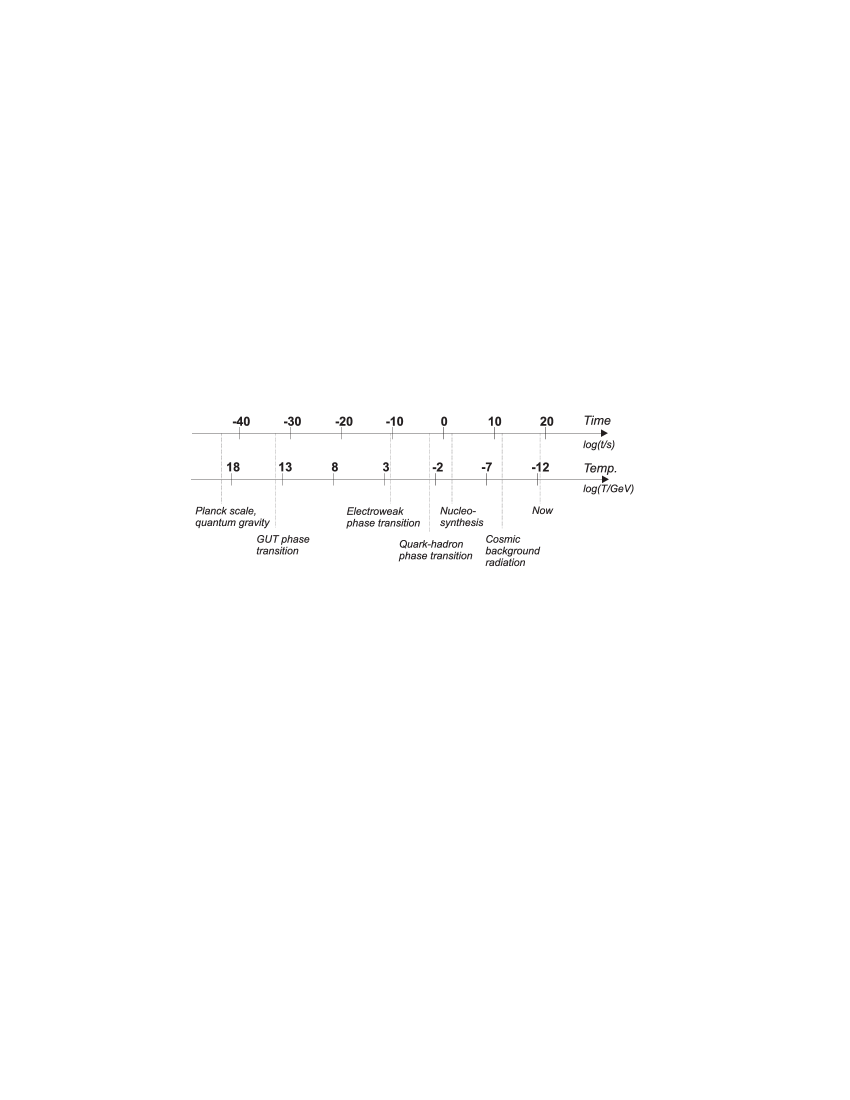
Figure 7.1: Thermal history of the Universe.

At $t\sim 10^{-43}$ s when the temperature was $T\sim 10^{19}$ GeV, (the ”Planck” temperature), quantum gravity effects were still important. At this time, the cosmic horizon was about the size of one particle, and since all mass/energy in the Universe was contained in this small volume, gravity was important. Hence, a theory of quantum gravity is needed to accurately describe this period. All efforts to construct such a model have, however, failed.

The fact that a quark-hadron transition took place in the early Universe is quite undisputed, although one may dwell about whether or not the quark phase was a QGP according to the standard particle physics description. The main reason for the recent interest in this transition is the implication the exact nature of the transition could have on the abundance of light elements in the Universe  [?]. However, it has also been argued  [?] that the exact QGP behaviour is not so crucial for the nucleosynthesis.

The actual transition is believed to have taken place by hadronic bubble growth inside the QGP. This was suggested by Witten  [?], and although some of his conclusions have been criticized  [?,?], the bubble nucleation mechanism is still in favour.

Witten suggested that at a temperature just below $T_{c}$, bubbles of hadronic matter appear. Since this corresponds to a first-order transition, a difference in energy density between the different phases appeared; a so-called latent heat. As such bubbles expand they expel heat, and a pressure equilibrium between the two phases makes it possible for them to coexist.

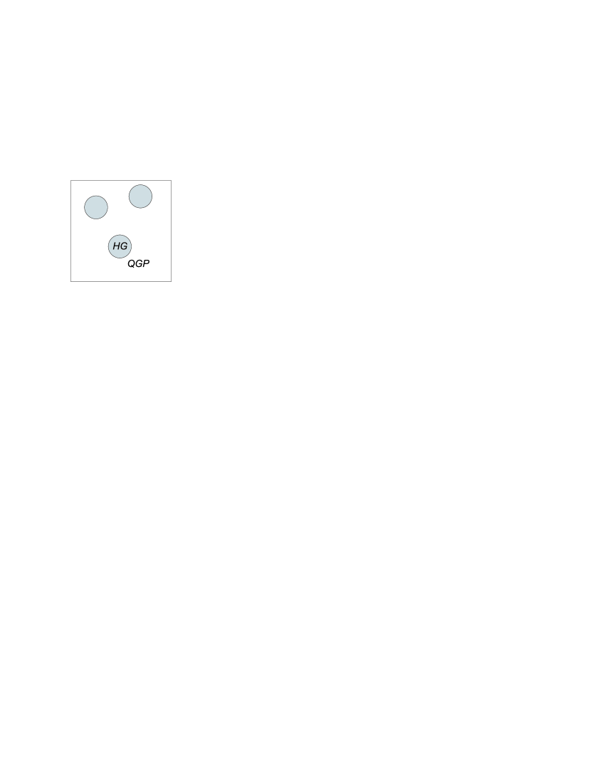
Figure 7.2: Bubbles of hadronic gas (HG) begin to form inside the QGP.

When the Universe expanded the hadronic bubbles also expanded and hence the formation of hadronic matter continued. When about 50% of the total volume had converted into hadronic matter, the QGP phase began to form bubbles inside a hadronic sea.

Figure 7.3: Here more than 50% of the total volume is occupied by hadronic gas, and the QGP shrinks to bubbles.

The further expansion of the Universe resulted in a loss of heat, while the QGP bubbles shrank until they finally disappeared. Thermal equilibrium seems to be a fair assumption for these rather slow processes  [?].

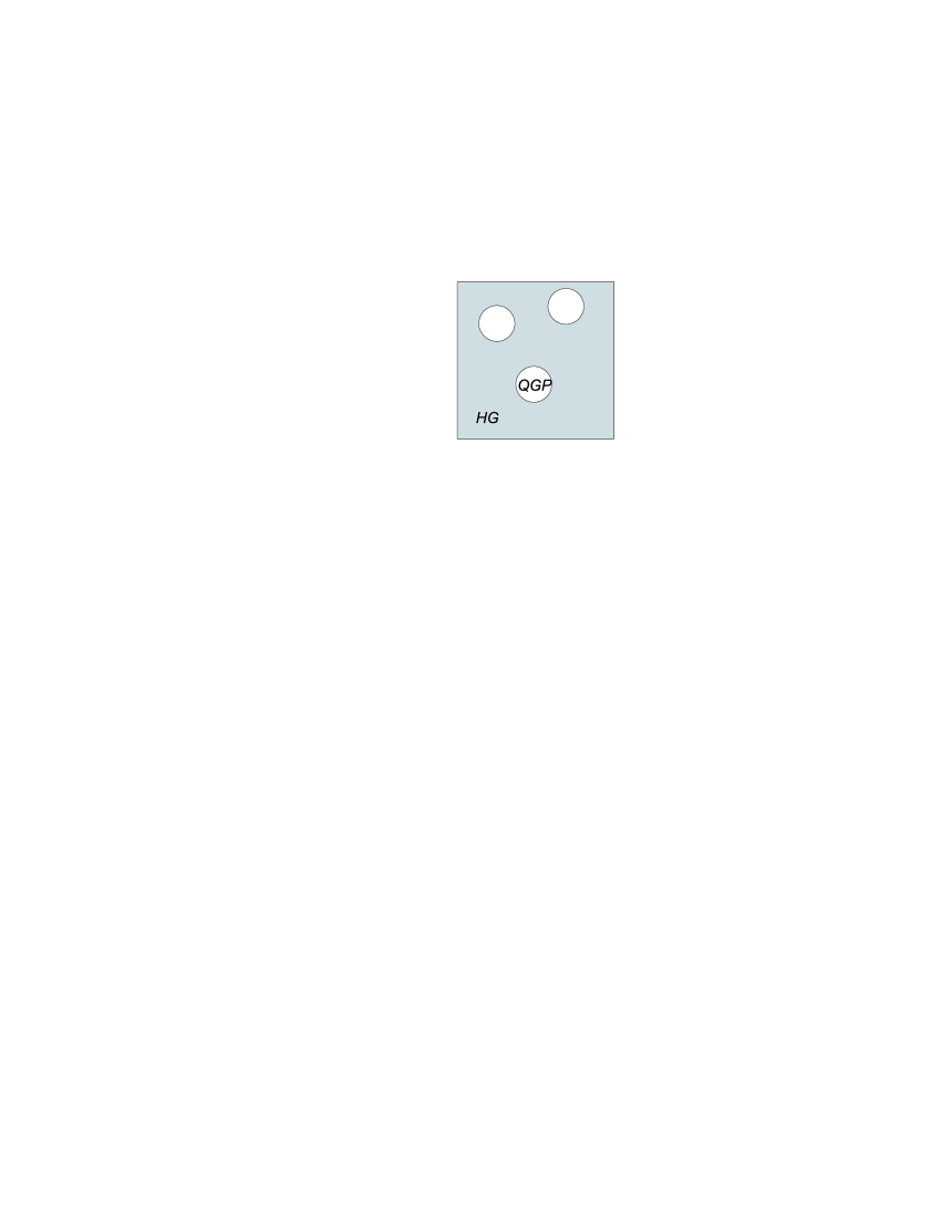
Figure 7.4: The further expansion of the Universe made the QGP bubbles shrink until they disappeared and led only the hadronic gas to participate in the primordial nucleosynthesis.

Witten also suggested the primordial QGP might have survived the quark-hadron transition and constitute some of the dark matter in the present Universe.

For a more thorough description of the present understanding of quark-hadron transition in the early Universe, see  [?].

7.2 QGP and compact stars

This section reviews the possible existence of QGP in compact stars, i.e., neutron stars and so-called quark stars. The material is to a large extent taken from Glendenning’s book ”Compact Stars”  [?].

The birthplace of a star is a cloud of interstellar gas. The cloud consists mostly of molecular hydrogen with varying density. The temperature in the cloud varies from $10$ K to $2000$ K in different spatial regions. When a local cluster of high-density regions experiences a perturbation, e.g. a shock wave, it will collapse gravitationally if the mass of the cloud is near the critical ”Jeans” mass. The compression continues until the internal thermal pressure balances the gravitational contraction energy. The core has then reached a high-enough temperature and density to fuse hydrogen into helium. The contracted cloud has become a main-sequence star.

The thermonuclear fusion continues even after all hydrogen in the core has been used. Now helium burns into carbon, and the fusion process continues until iron has been formed.

These processes do not depend on the mass of the star. The fusion rate is faster for heavy stars, but the processes are the same for all stars.

It is important to remember that fusion will start when and where the temperature and density is high enough in the star. At the beginning, fusion takes place only in the core, but the temperature and density in the outer layers of the star may be high enough for fusion to spread.

When fusion stops in the core of a light star of a few solar masses M_⊙, the thermal pressure decreases and the star starts to contract again. This increases the temperature and density all over the star, making hydrogen burn in the outer layers of the star. Such a star is called a red giant. All this repeats for helium, carbon etc. These processes can occur in an explosive manner, ripping away most of the star to form a planetary nebula. The remaining core of the star is too light to maintain fusion and forms a white dwarf with a surface temperature of around $8000$ K. It radiates energy for about 10¹⁰ years and thereafter becomes a black dwarf.

For a heavier star (m $>8$ M_⊙) the evolution is somewhat different from the period when iron has formed in the core. The burning process then continues in the outer layers of the star, adding to the iron content in the core. Gravity compresses the core until the electrons are captured by the protons; a process called inverse beta decay. The pressure in the core suddenly decreases and an enormous implosion occurs, which raises the central temperature in the core up to several tens of MeV ($\sim 10^{11}$ K). The core neutronizes, i.e., turns electrons and protons into neutrons. It decreases in volume, creating a shockwave that rips the outer regions of the star apart and creates a supernova in the sky. The total energy release is some 10⁴⁶ J. At this point the core has reached its final equilibrium state, composed of neutrons, protons, hyperons and leptons, and at the very centre, maybe a QGP.

If the mass of the star exceeds the so-called Oppenheimer-Volkoff mass limit, where the internal thermal pressure cannot balance the gravitational compression, a black hole is formed. There are other types of collapse suggested for the formation of a black hole. See  [?] for a review.

The density in the core of a neutron star is enormous ($\sim 10^{15}$ g/cm³), which means that the energy density inside a neutron star could be high enough for a QGP to form. Since the core has a higher density than the outer regions, a QGP core should be surrounded by a hadronic crust. Such stars are called hybrid stars. In the extreme case of a so-called quark star there is no hadron crust at all. For further reference, see chapter 8 in Glendenning’s book  [?].

Two possibilities exist concerning the existence of a QGP inside a hybrid star. It could have a pure QGP core with a distinct phase boundary against the hadronic crust. But there could also be a mixed phase with QGP and hadronic matter. Such a mixture could even be in the form of a crystalline lattice of various geometries, with the rarer phase immersed in the dominant one. Fig. 7.5 shows the internal structure of a hybrid star.

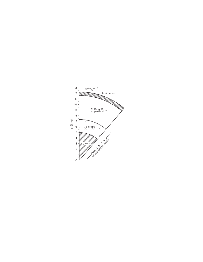
Figure 7.5: A section through a neutron star that contains an inner region of mixed phases including a crystalline lattice of deconfined and confined matter and a surrounding liquid of neutrons and leptons. A thin crust of heavy ions forms the stellar surface  [?].

Is it possible to model the internal structure of a hybrid star? With a bag constant $B^{1/4}=180$ MeV, and the coupling constants lying in the range of accepted values, the population of quarks, baryons and leptons will be as in Fig. 7.6.

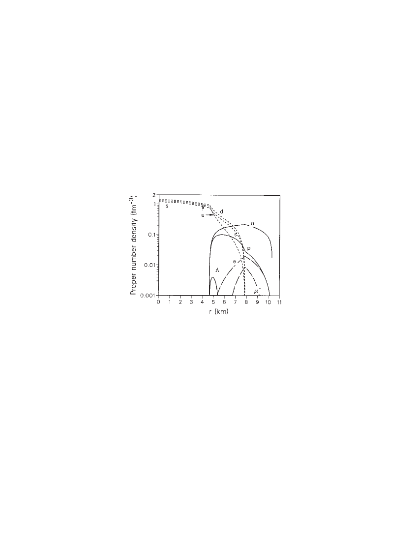
Figure 7.6: Population densities per unit volume in a hybrid star with mass 1.42 M_⊙ versus distance from the star centre  [?].

A neutron star is normally too cold to be directly observed, with one exception though; so-called pulsars. A pulsar is a highly magnetized neutron star that rotates very quickly and thus emits radiation along its axis of rotation, creating a pulsed signal with a very stable period. This was actually discovered in 1968 by Bell  [?], and the total number of discovered pulsars is now around 700. They are observed under various circumstances, usually as isolated sources, but sometimes in binary orbit with another white dwarf or neutron star.

Pulsars lie in the ms to s range with an average period of 0.7 s. They are very stable and the fastest pulsar known, the PSR 1913+16, has a period of $1.55780644887275\pm 0.00000000000003$ ms. The accuracy here is due to terrestrial time standards. The pulsars are therefore the most accurate clocks in the Universe.

As one might guess, there is a physical limit of the rotational velocity for a neutron star. When the centrifugal forces overcome the gravitational contraction, the star will break up and emit matter. For a neutron star of mass $1.44$ M_⊙ this limit corresponds to a period of  $0.3$ ms (assuming that the structure of the star is optimized to achieve maximum rotational frequency).

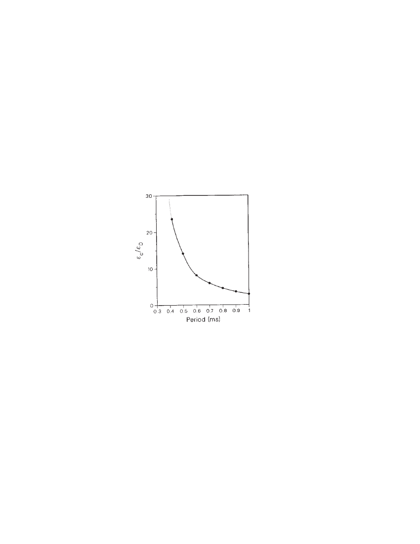
Figure 7.7: The least possible theoretical central density of a star with mass 1.44 M_⊙ required for stable rotation versus the rotational period. The energy density $\epsilon_{c}$ is normalized to $\epsilon_{0}$, the normal nuclear energy density  [?].

As can be seen in Fig. 7.7, the central density required to achieve submillisecond periods grows rapidly with decreasing period. One can thus conclude that matter under normal nuclear density is not able to keep the star together if the rotational period is of the order of $0.1$ ms. A reasonable assumption is therefore that if a submillisecond pulsar is discovered, its core must be denser than neutron matter, i.e., containing QGP in some form.

7.3 QGP and dark matter

The concept of cosmic dark matter is well established today. There are clear signals from different observational sources for discrepancies between the observed mass density and the dynamical behaviour of galaxies. The luminous mass simply cannot account for the observed rotations. This has been known for a long time, and many models have been proposed in terms of non-luminous ”dark” matter, which ultimately could account for 90% of the total mass of the Universe.

One such model was proposed by Witten  [?] in 1984. The dark matter was suggested to be leftover quark objects from the quark-hadron transition in the early Universe. Witten showed that under certain circumstances, QGP bags, or ”quark nuggets” as he called them, could survive to the present and form lumps of quark matter of size $\sim 10$ cm with a density of $\sim 10^{15}$ g/cm³.

There are more recent, and detailed, analyses of Witten’s idea. Madsen argued  [?] that QGP bags with baryon number A$<10^{35}$ cannot be dark-matter candidates. Alan, Raha and Sinha  [?] claimed that QGP bags with baryon number 10${}^{39}\leq A\leq 10^{49}$ are cosmologically stable and could solve the dark matter problem and even close the Universe gravitationally.

Explaining dark matter with QGP objects is appealing in the sense that it relies on the well-established idea that all nuclear matter was once in the form of QGP.

Chapter 8 Stability of cosmic QGP objects

8.1 Introduction

The second part of this thesis is an investigation of the possibility of stable QGP bags. These bags are assumed to be leftovers from the quark-hadron transition in the early Universe, following Witten’s idea  [?]. The basic idea is that if a pressure equilibrium occurs at the edge of the QGP bag, the bags could be stable. The dominant decay mechanism for a QGP is cooling by expansion and then hadronization, but if a pressure equilibrium would be present at the edge of the bag, no expansion would take place and the QGP would be stable. This possibility opens up new ways of explaining astrophysical phenomena such as dark matter and gamma-ray bursts.

This investigation can be divided into two parts:

• To determine the size where the gravitational pressure balances the other pressures occurring at the edge of the bag.

• To determine the corresponding QGP mass and compare the result with the Schwarzschild radius.

The calculations necessary to achieve these goals will be performed in several different configurations, varying the equation of state in different ways.

The question of quark matter stable against gravitational collapse have been investigated before, in the sense of stable quark or hybrid stars, e.g.  [?,?]. Compared to those models, the present work is built on similar equations of state, but with a different formation mechanism, since it assumes that the QGP objects are primordial.

8.2 The model

The model used for the stable QGP bag is simple. Four different pressures exist:

• A gravitational pressure.

• A vacuum pressure, characterized by the bag constant $B$.

• A kinetic pressure, from the motion of the quarks.

• A Fermi pressure of the quarks.

The kinetic pressure is identically zero if the temperature is zero. If a stable solution is to be found some kind of repulsive force must be taken into account. This is the degeneracy pressure of the quarks. The total pressure in the QGP bag will be divided into three parts:

$$p_{t}=p_{dg}+p_{k}-B.$$ (8.1)

$B$ is the negative (inward acting) vacuum pressure and $p_{k}$ is the outward kinetic pressure. $p_{dg}$ stands for the sum of the gravitational and the degenerate (Fermi) pressure. The total pressure $p_{t}$ will start at some value $p_{c}$ at the centre of the bag and decline to zero at the edge of the bag.

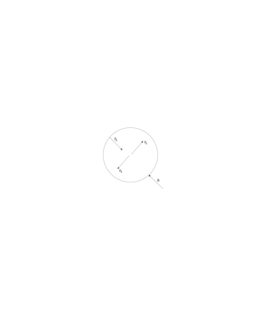
Figure 8.1: Phenomenological picture of the pressures acting on the QGP bag.

The actual calculations rest upon certain approximations and assumptions:

• The quarks in the QGP bag are $u$, $d$ and $s$ quarks, all taken to be massless.

• The plasma is taken to be a perfect fluid, i.e., the pressure is isotropic in the rest frame of each fluid element so that shear stress and heat transport can be neglected.

• The plasma is assumed to behave like a mixture of relativistic boson and fermion gases (gluons and quarks).

• The quark-hadron transition in the early Universe was a first-order transition.

• The metric used to describe a static spherical star can also be used to describe a QGP bag, i.e., the so-called Tolman-Oppenheimer-Volkoff eq. (9.1) is valid for a QGP bag.

• One of the parameters needed to be set at each calculation is the central pressure, $p_{c}$. The interesting range of this parameter is assumed to begin at the pressure equivalent to normal nuclear energy density, $\varepsilon_{nuc}\sim 170$ MeV/fm³ (corresponding to $\sim 3\cdot 10^{14}$ g/cm³).

• No decay process other than cooling by expansion and later hadronization is taken into account.

Chapter 9 The crucial equations

9.1 The Tolman-Oppenheimer-Volkoff equation

The standard equation describing the interior of a compact star is the Tolman-Oppenheimer-Volkoff (TOV) equation  [?]. It is derived from the Einstein field equations with a static, spherically symmetric metric governing the gravitational field for a static spherical star. In addition, the mass-energy tensor for the system is taken to represent a static perfect fluid. In the original calculations, the energy density and the pressure were taken to be zero outside the star. This leads to a boundary matching where the mass, integrated from the centre of the star to the edge, is set to be equal to the mass term in the external Schwarzschild metric.

However, when applying this formalism to an MIT bag, with its external vacuum pressure $B$, the energy density outside the bag will be $4B$. This seemingly strange assumption, inherent to the MIT bag model, does not significantly influence the metric.

The TOV equation is derived from the assumption of a static spherical star taken as a perfect fluid. It is derived in many textbooks in general relativity, e.g. in  [?]. It results in the following set of equations:

$$\frac{dp}{dr}=-\frac{[\epsilon(r)+p(r)][m(r)+4\pi r^{3}p(r)]}{r[r-2m(r)]},$$ (9.1)

$$\frac{dm(r)}{dr}=4\pi r^{2}\epsilon(r),\hskip 28.45274ptm(r)=4\pi\int_{0}^{r}\epsilon(r^{\prime})r^{\prime}{}^{2}dr^{\prime},$$ (9.2)

$$p(r=0)=p_{c},$$ (9.3)

$$p(r=R)=0.$$ (9.4)

These equations are expressed in gravitational and natural units, $c=\hbar=G=1$. $p$ is the total pressure, $\epsilon$ is the energy density, $m$ is the mass and $r$ is the radial coordinate.

The TOV equation requires just a static spherical mass-energy distribution and a perfect fluid. It does not depend on a certain equation of state that relates energy density and pressure.

9.2 The equation of state

The equation of state for a non-interacting QGP consisting solely by $u$ and $d$ quarks along with gluons was discussed in section 5.1. Allowing also $s$ quarks changes the equation of state somewhat. The pressure is, as previously stated, divided into four parts, where the kinetic part is derived for a mix between three fermion gases and one boson gas. These circumstances change the equation of state to

$$\epsilon(r)=3p_{t}(r)+4B.$$ (9.5)

The kinetic pressure is now with three quark flavours $(f)$:

$$p_{k}=\frac{8\pi^{2}}{45}T^{4}+\sum_{f}\left(\frac{7}{60}\pi^{2}T^{4}+\frac{1}{2}T^{2}\mu_{f}^{2}+\frac{1}{4\pi^{2}}\mu_{f}^{4}\right),$$ (9.6)

and the chemical potential $\mu_{f}$ is given for each quark flavour. When taking the lowest-order gluon interaction into account, the kinetic pressure changes into

$$p_{k}=\frac{8\pi^{2}}{45}T^{4}\left(1-\frac{15\alpha_{s}}{4\pi}\right)+\sum_{f}\left[\frac{7}{60}\pi^{2}T^{4}\left(1-\frac{50\alpha_{s}}{21\pi}\right)+\right.$$ (9.7)

$$\left.+\left(\frac{1}{2}T^{2}\mu_{f}^{2}+\frac{1}{4\pi^{2}}\mu_{f}^{4}\right)\left(1-\frac{2\alpha_{s}}{\pi}\right)\right].$$

This expression has been derived in  [?,?,?]. Here one can obviously study also the case when quarks do not interact, by setting $\alpha_{s}=0$.

After introducing $p_{t}$ into the TOV equation one gets

$$\frac{dp_{t}}{dr}=-\frac{\left(4p_{t}+4B\right)\left[4\pi\int_{0}^{r}\left(3p_{t}+4B\right)r^{\prime}{}^{2}dr^{\prime}+4\pi r^{3}p_{t}\right]}{r\left[r-2\cdot 4\pi\int_{0}^{r}\left(3p_{t}+4B\right)r^{\prime}{}^{2}dr^{\prime}\right]}$$ (9.8)

This integro-differential equation cannot be solved analytically, and basic numerical methods will be used in the following calculations.

Chapter 10 The method

10.1 The algorithm

Equation (9.8) is solved with two simple numerical algorithms. The derivative is changed according to

$$\frac{dp}{dr}\rightarrow\frac{p_{i+1}-p_{i}}{h},$$ (10.1)

and the integral is changed into

$$4\pi\int_{0}^{r}\left(3p_{t}+4B\right)r^{\prime}{}^{2}dr^{\prime}\rightarrow 4\pi\frac{h}{2}\cdot\left\{[p_{t}(0)+4B]\cdot 0^{2}+2[p_{t}(h)+\right.$$ (10.2)

$$\left.+4B]\cdot h^{2}+2[p_{t}(2h)+4B]\cdot(2h)^{2}+...+[p_{t}(nh=r)+4B]\cdot r^{2}\right\},$$

where $h$ is the constant step length. rThese discretizations change the TOV equation into

$$\frac{p_{i+1}-p_{i}}{h}=-\frac{\left(4p_{i}+4B\right)\left(\sum_{int}+4\pi r_{i}^{3}p_{i}\right)}{r_{i}\left(r_{i}-2\sum_{int}\right)},$$ (10.3)

where the integral approximation is denoted $\sum_{int}$.

As can be seen, there is a singularity at $r_{i}=0$. This makes it impossible to calculate $p(r=h)$ from eq. (9.8). This problem is not new, and methods have been developed to cope with it. A polynomial expansion will be used for the first step, i.e., in calculating $p(r=h)$, so that $p(r)=\sum_{j}p_{j}r^{j}$. Hence near $r=0$,

$$p=p(\epsilon_{c})+\left(p_{c}\Gamma_{c}/\epsilon_{c}\right)\left(\epsilon-\epsilon_{c}\right)+...\hskip 5.69046pt.$$ (10.4)

$\Gamma_{c}$ is the ”adiabatic index” $d[ln(p)]/d[ln(\epsilon)]$ evaluated at $\epsilon=\epsilon_{c}$, which also can be put on the form $dp/d\epsilon$ taken at the same energy density $\epsilon_{c}$. This expansion can now be written as

$$p(r)\approx p_{c}-2\pi\left(\epsilon_{c}+p_{c}\right)\left(p_{c}+\frac{1}{3}\epsilon_{c}\right)r^{2}+...,$$ (10.5)

so that $p(0)=p_{c}$, and $p(h)$ can be calculated. The resulting formula

$$p_{i+1}=p_{i}-\frac{h\left(4p_{i}+4B\right)\left(\sum_{int}+4\pi r^{3}p_{i}\right)}{r_{i}\left(r_{i}-2\sum_{int}\right)}$$ (10.6)

is to be iterated until the pressure $p_{t}=0$ is reached at some radius $r$, containing the full mass $(\sum_{int})$.

A scaling procedure has been used. All involved quantities are in km. This is possible by using gravitational and natural units:

$$\begin{array}[]{ccc}\left[p\right]&=&1/\mbox{km}^{2},\\ \left[\epsilon\right]&=&1/\mbox{km}^{2},\\ \left[T\right]&=&1/\sqrt{\mbox{km}},\\ \left[\mu_{f}\right]&=&1/\sqrt{\mbox{km}},\\ \left[r\right]&=&\mbox{km},\\ \left[B\right]&=&1/\mbox{km}^{2},\\ \left[m\right]&=&\mbox{km}.\end{array}$$

The following relationships hold:

$$B^{1/4},T,\mu_{f}:1\mbox{ MeV}=1\cdot\left(\frac{2.6115\cdot 10^{-4}}{(197.33)^{4}}\right)^{1/4}=6.4421\cdot 10^{-4}\,1/\sqrt{\mbox{km}},$$ (10.7)

$$\epsilon,p:1\mbox{ MeV/fm}^{3}=1\cdot\frac{2.6115\cdot 10^{-4}}{197.33}=1.3234\cdot 10^{-6}\,1/\mbox{km}^{2},$$ (10.8)

$$m:1\mbox{ kg}=1\cdot\frac{1.4766}{1.989\cdot 10^{30}}=7.4238\cdot 10^{-31}\mbox{ km}.$$ (10.9)

When using the scaling expressed above, the normal nuclear density $\varepsilon_{nuc}=3\cdot 10^{14}$ g/cm³ $\approx 170$ MeV/fm³ becomes $\epsilon_{nuc}\approx 2.2\cdot 10^{-4}$ 1/km² and bag constant $B=(150)^{4}$ (MeV)⁴ becomes $B\approx 8,7\cdot 10^{-5}$ 1/km².

10.2 Numerical stability and errors

The difference formula (10.1) for the derivative has an error of order $O(h)$, while that of the integral approximation has an error of order $O(h^{2})$. It is in principle possible to reduce the step size $h$, but it is then possible that one has to use the series solution, eq. (10.5), to determine the pressure close to the singularity, i.e., more than one step out of $r=0$.

When it comes to the stability criterion of the iteration procedure no theoretical examination has been made. The approach here has been to reduce the step size by 50% as long as significant differences, ($>1$%), remained between two iterations in the mass/radius relationship for the QGP bag. The final step size was $10$ m, i.e., $h=0.01$, which proved to be a suitable compromise between accuracy and CPU time.

10.3 Parameter variations

In the calculations there are seven variable parameters; $B,\alpha_{s}$, $T$, $\mu_{u}$, $\mu_{d}$, $\mu_{s}$ and $p_{c}$. The central pressure has been varied between $1.7-1.3\cdot 10^{5}$ times the corresponding normal nuclear density. The temperature has been varied between 0 and 2000 MeV, ($10^{12}$ K). No significant change in the bag size was caused by this variation of temperature. The same is true for the chemical potentials $\mu_{u}$, $\mu_{d}$ and $\mu_{s}$. The strength of the QCD interaction, $\alpha_{s}$ has been varied between 0 and $2.5$, which did not alter the bag size significantly. The only important variation that did alter the bag size (apart from that of the central pressure) was in the bag constant. The value of $B^{1/4}$ was varied between 120 and 180 MeV.

Chapter 11 Results and discussion

11.1 Results

When calculating the stable configurations for these QGP objects, a stability criterion built into the TOV equation must be considered. This is known as Le Chatelier’s principle and can be formulated as  [?]

$$\frac{\partial M(\epsilon_{c})}{\partial\epsilon_{c}}>0.$$ (11.1)

When applying this condition to the results presented here, the number of stable configurations is limited. As shown in Fig. 11.1, three regions in the range of the applied central energy density $\epsilon_{c}$ allow stable configurations.

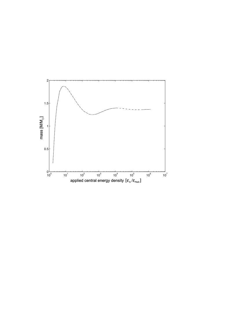
Figure 11.1: Mass vs. applied central energy density. Stable configurations occur only in the density intervals with the full-drawn line. The parameter values are $B^{1/4}=150$ MeV, $T=0$ MeV, $\mu_{u},\mu_{d},\mu_{s}=0$ and $\alpha_{s}=0$.

The first region is only interesting in the upper part, since at lower $\epsilon_{c}$, a QGP will not form. In the second region, $\epsilon_{c}$ is far above the QGP transition allowing stable configurations to occur. One should notice that at these $\epsilon_{c}$ values, the chemical potential for the $c$ quark is the same order of magnitude as its mass and therefore, the $c$ quark could be present in the centre of the QGP. This implication is not included in the calculations. The small third region, represents central densities about a thousand times higher than those in the Universe at the time of the quark-hadron transition.

Presenting the integration of the TOV equation in a mass-radius diagram normally results in a spiral-like curve. This is true also for the formalism presented here, as shown in Fig. 11.2.

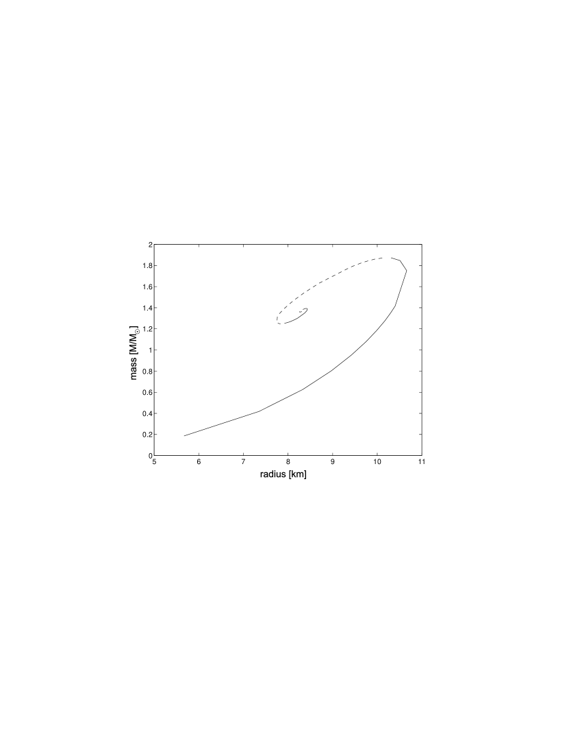
Figure 11.2: This plot shows stable (full line), and unstable (hatched line) configurations of the QGP bag. The parameter values are $B^{1/4}=150$ MeV, $T=200$ MeV, $\mu_{u},\mu_{d},\mu_{s}=0$ and $\alpha_{s}=0$. The central pressure is varied from $10^{-5}$ to $100$ km^-2, corresponding to a central energy density of $1.7$ to $1.3\cdot 10^{6}$ times $\varepsilon_{nuc}$.

If a QGP bag is to be stable, i.e., to be able to exist under a cosmological period of time, the temperature should be zero so that no thermal photons are emitted. If the temperature is set to zero in the calculations no visible change in the mass-radius relationship occurs within the accuracy of the iterative procedure, i.e., with a step in $r$ of 10 m.

The eq. (9.7) for the kinetic pressure $p_{k}$ does not depend much on the strong coupling constant $\alpha_{s}$, even for $\alpha_{s}$ values up to 2. Consequently, the mass-radius relationship is, in practice, independent of $\alpha_{s}$. The same result is achieved when varying the chemical potentials of the quarks. The only parameter variation that influences the mass-radius relationship substantially is the bag constant as can be seen in Fig. 11.3.

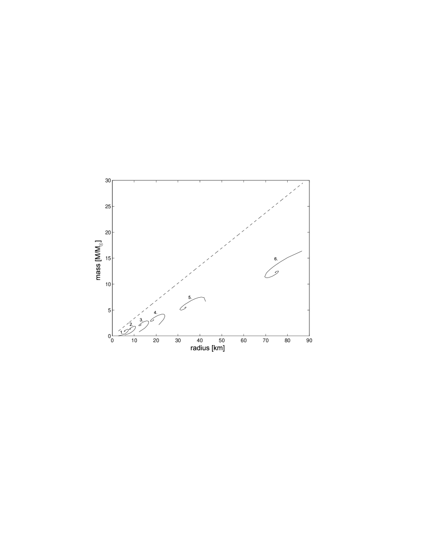
Figure 11.3: The mass-radius relation for varying bag pressure B (full line): B^1/4=180 MeV (curve 1.), 150 MeV (2.), 120 MeV (3.), 100 MeV (4.), 75 MeV (5.) and 50 MeV (6.). The hatched line corresponds to the Schwarzschild limit. All other parameter values are the same as in Fig. 11.2.

With the choice of parameter values in Fig. 11.2, it is obvious that one has two possible maxima regarding the mass of the bag. One lies around $10.5$ km with a mass about 1.9 M_⊙. This is achieved when the applied central energy density is about 10 $\epsilon_{nuc}$. The other lies at $8.5$ km with a mass about 1.4 M_⊙. Here, the applied central energy density is roughly 10⁴ $\epsilon_{nuc}$.

Using the basic formula for the Schwarzschild mass-radius relationship, $r_{s}=2Gm/c^{2}$, it is improbable with a gravitational collapse into a black hole, even at maximum mass configurations.

Figure 11.4: The same results as in Fig. 11.2 complemented with the mass-radius relation corresponding to the Schwarzschild radius (upper hatched line).

One might ask if there is any internal part that has a mass-radius relationship near that given by the Schwarzschild relation. One then needs to look at the energy density profile of the bag and compare the integrated mass with the Schwarzschild mass. No such situation appears with reasonable parameter values.

When varying the bag pressure $B$, as done in Fig. 11.3, the regions in $\epsilon_{c}$ resulting in stable mass-radius configurations is slightly shifted. One can also see, that significant changes in $B$ affect the mass-radius configurations, but not in a way that makes gravitational collapse more probable. The value of $B$ is traditionally taken from quantum-mechanical calculations involving the MIT bag model, where $B$ has been adjusted to make the calculated hadron masses agree with experimental data. In this thesis, the same values are used in a vast extrapolation to macroscopic objects, which is customary in astrophysical applications of the MIT bag model. However, one cannot be certain that the value of $B$ is the same regardless of external circumstances. In the calculations presented here, it is assumed that $B$ does not alter with the outside metric. The possibility that non-Euclidian geometry change the value of $B$ is not examined.

11.2 Discussion

Based on these calculations, one can conclude that a QGP bag obeying the chosen equation of state has a radius of either 7.5 - 8.5 km with mass 1.2 - 1.4 M_⊙ or 9 - 10 km with mass 1.6 - 1.8 M_⊙, while still being stable against evaporation and gravitational collapse. This result agrees with other quark matter stability calculations  [?,?]. The size and mass of these bags make them interesting as dark matter candidates as well as possible sources for gamma-ray bursts  [?].

The calculations also show that the connection between $\epsilon_{c}$ and the average energy density is rather weak, at least when $\epsilon_{c}>100\,\epsilon_{nuc}$. At high $\epsilon_{c}$, the energy density drops very fast with increasing radius close to the centre and assumes a behaviour rather similar to other, lower $\epsilon_{c}$ configurations, further out. This fact could be due to numerical errors close to the centre and remains to be investigated.

One circumstance that seriously could affect the possibility for QGP bags to survive the quark-hadron transition is the cosmic horizon size at the time of the transition, i.e., $10^{-5}$ s after Big Bang. At this time,  [?] states that the radius of the Universe was about $10^{-11}$ times the present size, i.e., about $10^{12}$ km.

The standard model in cosmology states that the average density in the Universe at the transition was about $10^{20}$ kg/m³. It is possible that local density fluctuations could have created regions that contained QGP at a considerably higher density than the average at the time of the transition. These regions later expanded with the Universe and possibly split up into smaller regions of QGP when fluctuations inside the region started local hadronization processes. Gravity retarded the expansion of these regions and the size necessary for a stable QGP bag could have been achieved. This process, when gravity counteracts the spatial expansion is a dynamical process that would be very interesting to look further into. Also, it would be of crucial importance to know if a QGP can exist in the intermediate density region between $\epsilon_{nuc}$ and a few times $\epsilon_{nuc}$. This region is considered to lie below the density needed to create a QGP out of compressed nuclei. However, such investigations lie beyond the scope of the present thesis.

Acknowledgements

I wish to thank my supervisor, Professor Sverker Fredriksson at the Division of Physics, Luleå University of Technology for encouragement, guiding and support, and Claes Uggla, Associate Professor at the same division for introducing me to some of the tools used in my calculations, especially in general relativity.

Appendix A Chiral symmetry

This Appendix on chirality and chiral symmetry follows roughly Donoghue, Golowich and Holstein  [?].

If one lets $\psi(x)$ be a solution to the Dirac equation for a massless particle:

$$i\not{\!\partial}\psi=0$$ (A.1)

and multiply this equation from the left by $\gamma_{5}$, one can use the anticommutativity with $\gamma^{\mu}$ to obtain

$$i\not{\!\partial}\gamma_{5}\psi=0.$$ (A.2)

The following combinations can be formed:

$$\psi_{L}=\frac{1}{2}(1+\gamma_{5})\psi,\hskip 42.67912pt\psi_{R}=\frac{1}{2}(1-\gamma_{5})\psi.$$ (A.3)

The quantities $\psi_{L}$ and $\psi_{R}$ are solutions of fixed chirality, in this case also called handedness. For a massive particle moving with precise momentum, these solutions correspond to the spin of the particle being, respectively, antialigned (left-handed) and aligned (right-handed) relative to the momentum.

The matrices $\Gamma_{LR}=(1\pm\gamma_{5})/2$ are chirality projection operators, fulfilling

$$\Gamma_{L}+\Gamma_{R}=1$$

.

(A.4)

Chirality is a natural label to use when referring to massless fermions thanks to its Lorentz invariance. A left-handed particle is left-handed to all observers. A physical example of this is the neutrino in the standard model. Neutrinos are left-handed chiral particles, i.e., if they are massless. There is no evidence for right-handed neutrinos.

Chirality is easy to add to the Lagrangian formalism. The Lagrangian for a non-interacting massless fermion is

$$L=i\overline{\psi}\not{\!\partial}\psi$$ (A.5)

or

$$L=L_{R}+L_{L}=i\overline{\psi}_{L}\not{\!\partial}\psi_{L}+i\overline{\psi}_{R}\not{\!\partial}\psi_{R}.$$ (A.6)

These Lagrangian densities are invariant under the global chiral phase transformation

$$\psi_{L,R}(x)\rightarrow\exp(i\alpha_{L,R})\psi_{L,R}(x),$$ (A.7)

where the phases $\alpha_{L,R}$ are constant and real-valued. Hence the Lagrangian density for massless particles has a chiral symmetry. If we use the famous Noether’s theorem we can associate conserved particle number current densities

$$J_{L,R}^{\mu}=\overline{\psi}_{L,R}\gamma^{\mu}\psi_{L,R}\hskip 28.45274pt(\partial_{\mu}J_{L,R}^{\mu}=0)$$ (A.8)

with this invariance. These chiral current densities form the basis for the vector current $V^{\mu}(x)$:

$$V^{\mu}=J_{L}^{\mu}+J_{R}^{\mu}$$ (A.9)

and the axial vector current $A^{\mu}(x)$:

$$A^{\mu}=J_{L}^{\mu}-J_{R}^{\mu}.$$ (A.10)

It is now possible to construct conserved chiral charges:

$$Q_{L,R}(t)=\int d^{3}xJ_{L,R}^{0}(x),$$ (A.11)

and these represent the number operators for the chiral fields $\psi_{L,R}$.

The vector charge $Q=Q_{L}+Q_{R}$ is the total number operator; whereas the axial vector charge, $Q_{5}=Q_{L}-Q_{R}$, is the number operator of the difference above. These charges simply count the sum and the difference of the left-handed and the right-handed particles.

The $u$ and the $d$ quark have masses far below the QCD scale parameter $\Lambda\simeq 0.2$ GeV which makes the assumption that $m_{u}\approx m_{d}\approx 0$ quite reasonable. It is even a fairly good approximation to treat the $s$ quark as massless, at least if the temperature (in energy units) is comparable to the mass of the $s$ quark. Due to the connection between mass and chiral symmetry shown in eqs. (A.1-A.3), chiral symmetry is not present as long as the fermions have mass.

When referring to QGP, I have previously stated that chiral symmetry is restored in the phase transition to QGP. This is only approximately so because the quarks inside the plasma are not massless. However, since the temperature and the scale parameter $\Lambda$ is roughly $200$ MeV, the assumption that $m_{u}\approx m_{d}\approx m_{s}\approx 0$ is fairly reasonable. The true chiral symmetry restoration also depends on the fact that the quark condensate expectation value vanishes at the phase transition. With these approximations, chiral symmetry is said to be restored in the QGP phase.

Appendix B The physics of phase transitions

This description of the role of symmetry-breaking in phase transitions is inspired by the book ”Cosmology” by Coles and Lucchin  [?].

The transition from some disordered phase to an ordered phase is labelled by a lowering of the symmetry in the system, which can be characterized by an order parameter $\Phi$. $\Phi$ is zero in the most disordered phase and rises when more ordered phases appear.

It is illustrative to take the solid/liquid phase transition as an example. The ordered phase has a low degree of (discrete) rotational symmetry, while the liquid gets an almost perfect rotational symmetry when the atoms move around at random. The order parameter $\Phi$ in this case represents the deviation of the spatial distribution of ions from the homogeneous distribution they have at $T>T_{C}$, the melting point. If $T>T_{C},\,\Phi=0$ and if $T<T_{C},\,\Phi>0$.

When $\Phi$ grows significantly, a symmetry-breaking transition has occurred. Such a transition can be caused either by an external influence, such as heating, or by a change of the system itself. Transitions due to external influences are called ”induced”, while those due to internal phenomena are ”spontaneous”. For the spontaneous symmetry-breaking processes it is convenient to consider the free energy of the system, $F=U-TS$, where $U$ is the internal energy, $T$ is the temperature and $S$ is the entropy. A condition for the system to be in an equilibrium state is that $F$ is at a minimum. At $T=0$ the free energy coincides with the internal energy. At $T>0$, whatever the form of $U$, an increase in $S$ leads to a decrease in $F$, and is therefore energetically favoured.

Phase transitions can be of two kinds; first- or second-order. If $\Phi$ rises continuously from zero when $T<T_{C}$ (the transition temperature), the transition is said to be of second-order, or continuous. If $\Phi$ jumps discontinuously to a non-zero value just below $T_{C}$ then the transition is of first order. Here, the entropy also exhibits a discontinuity at $T_{C}$. In a first-order transition, heat is adsorbed by the system in going from the low-temperature to the high-temperature phase. This heat is the latent heat, $Q_{L}=T_{C}\Delta S$, of the transition, where $\Delta S$ is the entropy change.

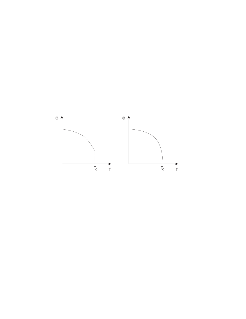
Figure B.1: Order parameter vs. temperature for a first-order (left) and a second-order (right) transition.

The QGP phase transition involves a spontaneous breaking of the chiral symmetry, i.e., chiral symmetry is broken in hadronic matter, but restored in the QGP. The order of the QGP phase transition has not been uniquely determined. Two massless flavours would generate a second-order transition  [?,?], while three massless flavours would give a first-order transition. In astrophysical calculations that involve a QGP phase transition, one often assumes that the transition is of first order.

Bibliography

- [1] F. Abe et al., Phys. Rev. Lett. 73, 225 (1994).
- [2] H. Fritzsch and M. Gell-Mann, Proc. XV Int. Conf. on High Energy Physics, Chicago-Batavia (1973).
- [3] Particle Data Group, Phys. Lett. 111B (1982).
- [4] B. Müller, The Physics of Quark-Gluon Plasma, Springer-Verlag (1985).
- [5] M. Gell-Mann, Phys. Rev. 125, 1067 (1962).
- [6] C.N. Yang and R.L. Mills, Phys. Rev. 96, 191 (1954).
- [7] K. Gottfried and V.F. Weisskopf, Concepts of Particle Physics, Oxford (1984).
- [8] P.N. Bogolioubov, Ann. Inst. Henri Poincaré 8, 163 (1967).
- [9] A. Chodos, R.L. Jaffe, K. Johnson, C.B. Thorn and V.F. Weisskopf, Phys. Rev. D 9, 3471 (1974).
- [10] K. Johnson, Acta Phys. Polon. B 6, 865 (1975).
- [11] P. Hasenfratz and J. Kuti, Phys. Rep. 40, 75 (1978).
- [12] G.E. Brown and M. Rho, Phys. Lett. 82B, 177 (1979).
- [13] S. Théberge, A.W. Thomas and G.A. Miller, Phys. Rev. D 22, 2838 (1980).
- [14] A.W. Thomas, S. Théberge and G.A. Miller, Phys. Rev. D 24, 216 (1981).
- [15] G. Kälbermann and J.M. Eisenberg, Phys. Rev. C 28, 1318 (1983).
- [16] R. Hagedorn, Nuovo Cim. Suppl. 3, 147 (1965).
- [17] S.I. Azakov, Research report Chalmers University of Technology 1986:39 (1986).
- [18] J.C. Collins and M. Perry, Phys. Lett. 34, 1353 (1975).
- [19] A.M. Polyakov, Phys. Lett. 72B, 224 (1977).
- [20] R.D. Pisarski and F. Wilczek, Phys. Rev. D 29, 338 (1984).
- [21] K. Rajagopal and F. Wilczek, Nucl. Phys. B 399, 395 (1993).
- [22] T. Blum, L. Kärkkäinen, D.Toussaint, S. Gottlieb, Phys. Rev. D 51, 5153 (1993).
- [23] M. Anselmino, E. Predazzi, S. Ekelin, S. Fredriksson and D.B. Lichtenberg, Rev. Mod. Phys. 65, 1199 (1993)
- [24] K. Geiger and B. Müller, Nucl. Phys. B 369, 600 (1992).
- [25] B. Andersson, G. Gustafson, G. Ingelman and T. Sjöstrand, Phys. Rep. 97, 91 (1983).
- [26] B. Müller, Rep. Prog. Phys. 58, 611 (1995).
- [27] K. Geiger, Phys. Rev. D 46, 4965 (1992).
- [28] A.H. Sørensen, Z. Phys. C 53, 95 (1992).
- [29] K.J. Eskola and X.N. Wang, Phys. Rev. D 49, 1284 (1994).
- [30] J. Letessier, A. Tounsi, U. Heinz, J. Sollfrank and J. Rafelski, Phys. Rev. Lett. 70, 3530 (1993).
- [31] F.R. Brown et al., Phys. Rev. Lett. 65, 2491 (1990).
- [32] K. Geiger and J.I. Kapusta, Phys. Rev. Lett. 70, 1920 (1993).
- [33] E.L. Shuryak and L. Xiong, Phys. Rev. D 70, 2241 (1993).
- [34] B. Kämpfer and O.P. Pavlenko, Phys. Lett. 289B, 127 (1992); Nucl. Phys. A 556, 351c (1994).
- [35] I. Kawrakov and J. Ranft, University of Leipzig report UL-HEP-92-08, (1992); K.J. Eskola and X.N. Wang, Phys. Rev. D 49, 4532 (1994).
- [36] M.T. Strickland, Phys. Lett. 331B, 245 (1994).
- [37] J. Kapusta, P. Lichard and D. Seibert, Phys. Rev. D 44, 2744 (1991); Nucl. Phys. A 544, 485C (1992); Phys. Rev. D 47, 4171(E) (1993).
- [38] D.K. Srivastava, B. Sinha, M. Gyulassy and X.N. Wang, Phys. Lett. 276B, 285 (1992).
- [39] S. Chakrabarty, J. Alam, D.K. Srivastava, B. Sinha and S. Raha, Phys. Rev. D 46, 3802 (1992).
- [40] J.P. Bailly et al., Phys. Lett. 195B, 609 (1987).
- [41] J. Rafelski and B. Müller, Phys. Rev. Lett. 48, 1066 (1982) [Erratum: ibid. 56, 2334 (1986)].
- [42] J. Rafelski, Phys. Rep. 88, 331 (1982).
- [43] P. Koch, B. Müller and J. Rafelski, Phys. Rep. 142, 167 (1986).
- [44] M. Gaździcki and S. Mrówczyński, Z. Phys. C 49, 546 (1991).
- [45] R. Lietava, Z. Phys. C 50, 107 (1991).
- [46] J.D. Bjorken, Acta Phys. Polon. B 23, 637 (1992).
- [47] C.M.G. Lattes, Y. Fujimoto and S. Hasegawa, Phys. Rep. 65, 151 (1980); G. Arnison et al., Phys. Lett. 122B, 189 (1983); G.J. Alner et al., Phys. Lett. 180B, 415 (1986); Phys. Rep. 154, 247 (1987); J.R. Ren et al., Phys. Rev. D 38, 1417 (1988); L.T. Baradzei et al., Nucl. Phys. B 370, 365 (1992).
- [48] T. Matsui and H. Satz, Phys. Lett. 178B, 416 (1986).
- [49] J.P. Blaizot and J.Y. Ollitraut, Phys. Lett. 199B, 499 (1987).
- [50] F. Karsch and R. Petronzio, Phys. Lett. 212B, 255 (1988).
- [51] P.V. Ruuskanen and H. Satz, Z. Phys. C 37, 623 (1988).
- [52] M.C. Chu and T. Matsui, Phys. Rev. D 37, 1851 (1988).
- [53] H. Satz, Nucl. Phys. A 488, 511 (1988).
- [54] T. Matsui, Z. Phys. C 38, 245 (1988).
- [55] J. Ftacnik, P. Lichard, N. Pišutova and J. Pišuit, Z. Phys. C 42, 139 (1989).
- [56] G. Röpke, D. Blaschke and H. Schultz, Phys. Rev. D 38, 3589 (1988).
- [57] S. Raha and B. Sinha, Phys. Lett. 218B, 413 (1989).
- [58] C. Baglin et al. (NA38 collaboration), Phys. Lett. 220B, 471 (1989); Phys. Lett. 251B, 465 (1990); Phys. Lett. 262B, 362 (1991); Phys. Lett. 268B, 453 (1991); Phys. Lett. 270B, 105 (1991).
- [59] S. Gavin, H. Satz, R.L. Thews and R. Vogt, Z. Phys. C 61, 351 (1994); S. Gavin, Nucl. Phys. A 566, 383c (1994).
- [60] H. Satz, preprint hep-ph/9706342 (1997).
- [61] T. Abbott et al., Phys. Rev. C 50, 1024 (1994).
- [62] T. Alber et al., Z. Phys. C 64, 195 (1994).
- [63] E. Anderson et al., Phys. Lett. 294B, 127 (1992); Phys. Lett. 327B, 433 (1994).
- [64] S. Abatzis et al., Nucl. Phys. A 566, 499c (1994); 566, 491c (1994); 566, 225c (1994); Phys. Lett. 316B, 615 (1993); D. Dibari et al., Nucl. Phys. A 590, 307c (1995).
- [65] J.B. Kinson et al., Nucl. Phys. A 590, 317c (1995).
- [66] M. Gaździcki et al., Nucl. Phys. A 590, 197c (1995).
- [67] J. Letessier, A. Tounsi and J. Rafelski, Phys. Lett. 292B, 417 (1992).
- [68] J. Letessier et al., Phys. Rev. Lett. 70, 3530 (1992).
- [69] J. Letessier, A. Tounsi, U. Heinz, J. Sollfrank and J. Rafelski, Phys. Rev. Lett. 70, 3530 (1993); Phys. Rev. D 51, 3408 (1995); J. Sollfrank, M. Gaździcki, U. Heinz and J. Rafelski, Z. Phys. C 61, 659 (1994).
- [70] J.W. Harris and B. Müller, review to be published in Ann. Rev. of Nucl. and Part. Sci. (1996), preprint available at hep-ph/9602235.
- [71] J. Applegate, C. Hogan and R. Scherrer, Astrophys. J. 329, 572 (1988).
- [72] D.N. Schramm, The Big Bang and other Explosions in Nuclear and Particle Astrophysics, p. 349 World Scientific (1996).
- [73] E. Witten, Phys. Rev. D 30, 272 (1984).
- [74] C. Alcock and E. Farhi, Phys. Rev. D 32, 1273 (1985).
- [75] C. Alcock and A.V. Olinto, Ann. Rev. Nucl. Part. Sci. 38, 1273 (1988).
- [76] J. Ignatius, University of Helsinki PhD thesis (1993).
- [77] N.K. Glendenning, Compact Stars, Springer (1997).
- [78] A. Hewish, S.J. Bell, J.D.H. Pilkington, P.F. Scott and R.A. Collins, Nature 217, 709 (1968).
- [79] J. Madsen, Phys. Rev. Lett. 26, 2909 (1988).
- [80] J. Alam, S. Raha and B. Sinha, preprint astro-ph/9704226 (1997).
- [81] J.F. Donoghue, E. Golowich and B. R. Holstein, Dynamics of the Standard Model, Cambridge University Press (1994).
- [82] P. Coles and F. Lucchin, Cosmology: the Origin and Evolution of Cosmic Structure, John Wiley (1995).
- [83] Y. Iwasaki et al., Phys. Rev. D 54, 7010 (1996).
- [84] J.E. Horvath and J.A. de Freitas Pacheo, preprint astro-ph/9611167 (1996).
- [85] S.B. Khadkikar, A. Mishra and H. Mishra, Mod. Phys. Lett. A, to appear.
- [86] J.R. Oppenheimer and G. Volkoff, Phys. Rev. 55, 377 (1939).
- [87] B. Schutz, A First Course in General Relativity, Cambridge University Press (1990).
- [88] S.A. Chin, Phys. Lett. 78B, 552 (1978).
- [89] J.I. Kapusta, Nucl. Phys. B 148, 461 (1979).
- [90] O.K. Kalashnikov and V.V. Klimov, Phys. Lett. 88B, 328 (1979).
- [91] S.B. Khadkikar, A. Mishra and H. Mishra, Mod. Phys. Lett. A 10, 2651 (1995).
- [92] B. Anoushirvani, D. Enström, S. Fredriksson, J. Hansson, P. Ökvist, A. Nicolaidis and S. Ekelin, to be published in the Proc. of the Joint Meeting of the Networks ”The Fundamental Structure of Matter” and ”Tests of the Electroweak Symmetry Breaking”, Ouranoupolis, Greece, May 1997, preprint available at astro-ph/9711346 (1997).
- [93] E.W. Kolb and M.S. Turner, The Early Universe, Addison Wesley (1990).