Analytic Perturbation Theory and
Renormalization Scheme Dependence
in $\tau$-decay

Abstract

We apply analytic perturbation theory in next-to-next-to-leading order to inclusive semileptonic $\tau$-decay and study the renormalization scheme dependence. We argue that the renormalization scheme ambiguity is considerably reduced in the analytic perturbation theory framework and we obtain a rather stable theoretical prediction.

I Introduction

The $\tau$-lepton is the only known lepton massive enough to decay into hadrons. Its semileptonic decays are very convenient for studying strong interactions at low energies, because nonperturbative contributions are rather small and one can apply the standard methods of quantum field theory. The measurement of the quantity $R_{\tau}$ allows one to extract the value of the strong coupling constant at a low energy scale. The comparison of this value with ones obtained at higher energies is an important test of the applicability of QCD perturbation theory at low energies.

The method usually used to calculate perturbative QCD contributions to quantities such as $R_{\tau}$ consists in rewriting the original expression, which involves integration over small values of momentum, by means of Cauchy’s theorem and thereby convert it into a contour integral in a region of relatively large momentum. But the occurrence of incorrect analytic properties of the perturbative approximation, such as the appearance of a ghost pole and an unphysical cut, make it impossible to exploit Cauchy’s theorem in this manner.

In this paper we will use analytic perturbation theory [1, 2], which provides a correlator $\Pi(q^{2})$  with the correct analytic properties. For example, the one-loop analytic running coupling constant $a_{\rm an}(q^{2})$ in this approach is given by

$$a_{\rm an}(q^{2})=\frac{2}{b}\left[\frac{1}{\ln{(-q^{2}/\Lambda^{2})}}+\frac{\Lambda^{2}}{\Lambda^{2}+q^{2}}\right],$$ (1)

where $a=\alpha_{s}/\pi$ and $b/2$ is the first $\beta$-function coefficient. It is clear that, unlike the standard perturbative expression, this one has no unphysical ghost pole and, therefore, possesses the correct analytic properties, arising from the Källen-Lehmann analyticity that reflects the principle of causality. The nonperturbative term which appears in the running coupling constant does not change the ultraviolet limit of theory. A distinguishing feature of this approach is the presence of a universal limit at $q^{2}=0$, independent of both the scale parameter $\Lambda$ and choice of renormalization scheme. This quantity turns out to be stable with respect to higher loop corrections.

In order to compare theoretical results with experimental measurements one has to estimate the uncertainty connected to the renormalization scheme dependence of the perturbative approximation. It is well known that at low energies this ambiguity becomes considerable (see, e.g., Ref. [3]). Analytic perturbation theory improves the situation and gives very stable results over a wide range of renormalization schemes, as has been demonstrated for the $e^{+}e^{-}$ annihilation ratio in Ref. [4].

We will perform the calculation of $R_{\tau}$ at the two- and three-loop levels and study the renormalization scheme dependence within analytic perturbation theory. All results will be compared with standard perturbative ones. This investigation is a continuation of the program initiated in Ref. [5].

II Problem of QCD parametrization of $R_{\tau}$

The ratio of hadronic to leptonic $\tau$-decay widths

$$R_{\tau}\equiv\frac{\Gamma(\tau^{-}\to\nu_{\tau}{\rm hadrons})}{\Gamma(\tau^{-}\to\nu_{\tau}l^{-}{\bar{\nu}}_{l})}$$ (2)

has the following theoretical representation

$$R_{\tau}=3\,S_{\rm EW}(|V_{ud}|^{2}+|V_{us}|^{2})(1+\delta_{\rm QCD}),$$ (3)

where $V_{ud}$ and $V_{us}$ are the CKM matrix elements, $S_{\rm EW}$ is the electroweak factor, and $\delta_{\rm QCD}$ is the pure QCD correction [6], which we will calculate perturbatively. It is convenient to introduce some definitions: ${\rm Im}\ \Pi\sim 1+r$ for the perturbative part of correlator $\Pi(q^{2})$ and $D\sim 1+d$ for the perturbative part of Adler function $D(q^{2})$. Then one can write $\delta_{\rm QCD}$  as an integral over timelike momentum $s$:

$$\delta_{\rm QCD}=2\int_{0}^{M_{\tau}^{2}}\frac{ds}{M_{\tau}^{2}}{\left(1-\frac{s}{M_{\tau}^{2}}\right)}^{2}\left(1+2\frac{s}{M_{\tau}^{2}}\right)r(s).$$ (4)

If one uses the standard perturbative approximation this integral is ill-defined because of unphysical singularities within the range of integration; standard perturbation theory (PT) fails. The most useful trick to rescue the situation is to appeal to analytic properties of the hadronic correlator $\Pi(q^{2})$ [6]. This opens up the possibility of exploiting Cauchy’s theorem by rewriting the integral in the form of a contour integral in the complex $q^{2}$-plane with the contour being a circle of radius $M_{\tau}^{2}$:

$$\delta_{\rm QCD}=\frac{1}{2\pi i}\oint_{|z|=M_{\tau}^{2}}\frac{dz}{z}{\left(1-\frac{z}{M_{\tau}^{2}}\right)}^{3}\left(1+\frac{z}{M_{\tau}^{2}}\right)d(z).$$ (5)

However, as noted, the transition to the contour representation (5) requires certain analytic properties of the correlator, namely, that it must be an analytic function in the complex $q^{2}$-plane with a cut along the positive real axis. The correlator parametrized by the running coupling constant in standard perturbation theory does not have this virtue [7, 5]. Moreover, a renormalization group analysis gives a running coupling constant determined in the spacelike region, whereas the initial expression (4) for $R_{\tau}$ contains an integration over timelike momentum. Thus, we are in need of some method of continuing the running coupling constant from the spacelike to the timelike region that takes into account the proper analytic properties of the running coupling constant. Because of this failure of analyticity Eqs. (4) and (5) are not equivalent in PT.

Nevertheless, if one uses Eq. (5) with the PT approximation for $d(z)$, thus calculating the contour integral in a naive way, a new problem will emerge. It is known that the lower the energy scale we consider, the greater the uncertainty there is related to the choice of renormalization scheme (RS). If one turns to the $D(q^{2})$-function, which can be extracted from the ratio $R_{e^{+}e^{-}}$ for $e^{+}e^{-}$ annihilation, one finds that the RS dependence of theoretical predictions is considerable [3]. At the energy scale around $M_{\tau}$ this uncertainty increases drastically. The transition to the contour integral softens this ambiguity, but it remains large. Moreover, as we noted, within PT this transition to the contour integral representation cannot be performed self-consistently. Therefore, there is no consistent method of calculating the inclusive decay of the $\tau$-lepton into hadrons in the framework of standard perturbation theory.

Recently, a new approach that eliminates the two problems described above has been proposed [1, 2]. This is the so-called analytic perturbation theory (APT), in which the hadronic correlator $\Pi(q^{2})$ has the correct analytic properties. In this approach, the $d_{\rm an}(q^{2})$ function, which is analytic in the cut $q^{2}$-plane, can be expressed in terms of the spectral density $\rho(\sigma)$, the basic quantity in APT (to distinguish APT and PT we have introduced subscripts “an” and “pt” instead of QCD)

$$d_{\rm an}(q^{2})=\frac{1}{\pi}\int^{\infty}_{0}\frac{d\sigma}{\sigma-q^{2}}\rho(\sigma).$$ (6)

We can write down some useful dispersion relations, which are consequences of the analytic properties of the correlator. The first one is

$$d(q^{2})=-q^{2}\int^{\infty}_{0}\frac{ds}{{(s-q^{2})}^{2}}r(s),$$ (7)

which is inverted by the following formula,

$$r(s)=-\frac{1}{2\pi i}\int^{s+i\epsilon}_{s-i\epsilon}\frac{dz}{z}d(z).$$ (8)

Here, the contour lies in the region of analyticity of the $D(q^{2})$-function. Then let us rewrite the last expression in terms of the spectral density $\rho(\sigma)$ [8]:

$$r_{\rm an}(s)=\frac{1}{\pi}\int^{\infty}_{s}\frac{d\sigma}{\sigma}\rho(\sigma).$$ (9)

If we substitute the last formula into integral (4), we can easily verify that the contour representation (5) holds [5]. Using the spectral representation (6), we can rewrite $\delta_{\rm an}$ in terms of $\rho(\sigma)$:

$$\delta_{\rm an}=\frac{1}{\pi}\int_{0}^{\infty}\frac{d\sigma}{\sigma}\rho(\sigma)-\frac{1}{\pi}\int^{M_{\tau}^{2}}_{0}\frac{d\sigma}{\sigma}{\left(1-\frac{\sigma}{M_{\tau}^{2}}\right)}^{3}\left(1+\frac{\sigma}{M_{\tau}^{2}}\right)\rho(\sigma).$$ (10)

The first term in this formula is simply the value $d_{\rm an}(0)$. Once an expression for $\rho(\sigma)$ is given, we can calculate the integral (10).

Consider $\delta_{\rm an}$ at the three-loop level. The running coupling constant $a=\alpha_{s}/\pi$ satisfies the NNLO renormalization group equation:

$$\mu^{2}\frac{da}{d\mu^{2}}=-\frac{b}{2}a^{2}(1+c_{1}a+c_{2}a^{2}).$$ (11)

In the modified minimal subtraction scheme, $\overline{\rm{MS}}$, for three active flavors, we have $b=9/2$, $c_{1}=16/9$ and $c_{2}^{\overline{\rm{MS}}}=3863/864$. The renormalization-group improved perturbation expansion for $d_{\rm pt}(q^{2})$ is given by

$$d_{\rm pt}(q^{2})=a(q^{2})[1+{d_{1}}a(q^{2})+d_{2}a^{2}(q^{2})].$$ (12)

In the following, values of ${d_{1}}$ and $d_{2}$ will be needed; in the $\overline{\rm{MS}}$-scheme they are $d_{1}^{\overline{\rm{MS}}}=1.6398$ and $d_{2}^{\overline{\rm{MS}}}=6.3710$ [9].

In the APT approach, the spectral density is defined as the imaginary part of the perturbative approximation to $d_{\rm pt}(q^{2})$ on the physical cut:

$$\rho(\sigma)=\varrho_{0}(\sigma)+d_{1}\varrho_{1}(\sigma)+d_{2}\varrho_{2}(\sigma),$$ (13)

where

$$\varrho_{n}(\sigma)={\rm Im}[a^{n+1}(\sigma+i\epsilon)].$$ (14)

The first of these spectral densities gives an analytic expression for the running coupling constant $a_{\rm an}(q^{2})$:

$$a_{\rm an}(q^{2})=\frac{1}{\pi}\int_{0}^{\infty}\frac{d\sigma}{\sigma-q^{2}}\varrho_{0}(\sigma).$$ (15)

This is what was called the spacelike running coupling constant in Ref. [5]. In the one-loop approximation it leads to Eq. (1).

For the following considerations, it is important that $d_{\rm an}(q^{2})$ and $a_{\rm an}(q^{2})$  have a universal limit at the point $q^{2}=0$. This limiting value, generally, is independent of both the scale parameter $\Lambda$ and the order of the loop expansion being considered. Because $d_{\rm an}(0)$ and $a_{\rm an}(0)$  are equal to the reciprocal of the first coefficient of the QCD $\beta$-function, they are also RS invariant (we consider only gauge- and mass-independent RSs). The existence of this fixed point will play a decisive role in the very weak RS dependence of our results.

The next point we should like to note is that the two approaches, APT and PT, coincide with each other in the asymptotic region of high energies. The procedure of implementing analyticity described above does not change the ultraviolet limit of the theory, i.e., $d_{\rm an}(q^{2})$  has the same asymptotic behavior as $q^{2}\rightarrow-\infty$ as the standard PT Adler function.

Therefore, the above gives a self-consistent framework in which we can estimate the $R_{\tau}$-ratio and extract from the measured value of $R_{\tau}$ the QCD scale parameter $\Lambda$.

III Renormalization scheme dependence

In this section we will investigate the RS dependence of the APT approach. The Adler function $d_{\rm an}$, as in PT, is parametrized by a set of RS parameters, but only two of them are independent. There is a RS invariant combination $\omega_{2}$ [11] of RS parameters that binds them:

$$\omega_{2}=c_{2}+d_{2}-c_{1}{d_{1}}-{d_{1}}^{2},$$ (16)

which in our case equals 5.2378. Here, $c_{1}$ is RS invariant in the class of schemes mentioned above. Thus, we can choose ${d_{1}}$ and $c_{2}$ as independent variables, which define the RS, and parametrize the QCD correction in terms of them.

To find $d_{\rm an}(q^{2})$ we use Eqs. (13), (14), and (6) and solve the transcendental equation for the running coupling constant on the physical cut lying along the positive real axis:

$$\frac{b}{2}\ln\left(\frac{-q^{2}}{\Lambda_{\overline{\rm{MS}}}^{2}}\right)-i\pi\frac{b}{2}=d_{1}^{\overline{\rm{MS}}}-{d_{1}}+\frac{1}{a}+c_{1}\ln\left(\frac{b}{2c_{1}}\right)+F^{(l)}(a),$$ (17)

where at the two-loop order

$$F^{(2)}(a)=c_{1}\ln\left(\frac{c_{1}a}{1+c_{1}a}\right),$$ (18)

and at the three-loop order

$$F^{(3)}(a)=F^{(2)}(a)+c_{2}\int^{a}_{0}\frac{dx}{(1+c_{1}x)(1+c_{1}x+c_{2}x^{2})}.$$ (19)

These expressions hold in any renormalization scheme.

It is necessary to extract $\Lambda_{\overline{\rm{MS}}}$ from the fit in the $\overline{\rm{MS}}$-scheme and after this procedure to pass on to other renormalization schemes with the RS-invariant parameter $\Lambda_{\overline{\rm{MS}}}$. To do the fit we took the values $V_{ud}=0.9752$, $V_{us}=0.2205$, $S_{\rm EW}=1.0194$ and $M_{\tau}=1.777$ GeV [12, 13]. For numerical estimations, we used the world average value $R_{\tau}=3.633\pm 0.031$ [14], which leads to the following value of the QCD scale parameter in three-loops: $\Lambda_{\overline{\rm MS}}^{\rm an}=871\pm 155$ MeV. The corresponding value of $d_{\rm an}(M_{\tau}^{2})$ is $0.1446\pm 0.0088$ and of $\alpha_{\rm an}(M_{\tau}^{2})$ is $0.3962\pm 0.0298$. To compare this result with the PT prediction we did the same fit using the contour integral representation (5) and got $\Lambda_{\overline{\rm MS}}^{\rm pt}=385\pm 27$ MeV, $d_{\rm pt}(M_{\tau}^{2})=0.1339\pm 0.0069$, and $\alpha_{\rm pt}(M_{\tau}^{2})=0.3371\pm 0.0141$. Thus, the values of the $D$-function are close to each other, but the value of $\Lambda_{\overline{\rm MS}}^{\rm an}$ in the APT approach is much larger than the one obtained in PT. As in Ref. [5], we found that this value is very sensitive to the value of $R_{\tau}$. In other words, $\delta_{\rm an}$ depends so slightly on $\Lambda_{\overline{\rm{MS}}}$ that a $0.9\%$ error in $R_{\tau}$ gives $18\%$ error in the value of $\Lambda_{\overline{\rm{MS}}}$. We illustrate this feature in Table 1. According to the table, when we change $M_{\tau}^{2}/\Lambda^{2}$ from 2.0 to 6.5 (corresponding to a variation of $\Lambda$ from 1.256 GeV to 0.697 GeV), $\delta_{\rm an}$ is only altered by about $20\%$. The sensitivity to $\Lambda_{\overline{\rm{MS}}}$ increases as $M_{\tau}^{2}/\Lambda^{2}$ gets smaller.

For comparison, we also include the two-loop result: $\Lambda_{\overline{\rm MS}}^{\rm an}=918\pm 151$ MeV, $d_{\rm an}(M_{\tau}^{2})=0.1431\pm 0.0084$, and the running coupling constant $\alpha_{\rm an}(M_{\tau}^{2})=0.3983\pm 0.0236$. The perturbative result is $\Lambda_{\overline{\rm MS}}^{\rm pt}=458\pm 31$ MeV, $d_{\rm pt}(M_{\tau}^{2})=0.140\pm 0.0067$, and $\alpha_{\rm pt}(M_{\tau}^{2})=0.3544\pm 0.0157$.

The reader should further note that the convergence properties of the APT series are much better than those of the PT case; in the improved scheme, the main contribution comes from the diagrams of lowest order. For example, the value of the three-loop APT correction to $d_{\rm an}(M_{\tau}^{2})$ is smaller than the corresponding PT contribution to $d_{\rm pt}(M_{\tau}^{2})$ by about a factor of four.

Having found $\Lambda_{\overline{\rm{MS}}}$, we will now study how $\delta_{\rm an}$ varies with a change of renormalization scheme. A natural way to do so is to supplement results in a certain scheme with an estimate of variability of predictions over a whole range of a priori acceptable schemes. To restrict this uncertainty one has to impose some requirement eliminating schemes with unnaturally large coefficients that would introduce large cancellations. It was proposed to calculate theoretical predictions over the set of schemes satisfying the condition [15]

$$|c_{2}|+|d_{2}|+c_{1}|{d_{1}}|+{d_{1}}^{2}\leq 2|\omega_{2}|,$$ (20)

which allows schemes with a degree of cancellation the same or smaller than what occurs in the scheme obeying the so-called principle of minimal sensitivity (PMS).

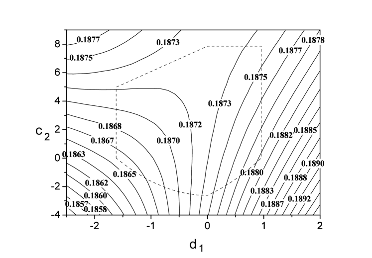
In the $\overline{\rm{MS}}$-scheme we adopt $\delta_{\rm an,pt}=0.1881$. Let us consider some points belonging to the domain described above and compare corresponding values of $\delta_{\rm pt}$. For example, suppose we choose the points $A=\left(-1.6183,0\right)$ and $B=\left(0.9575,0\right)$, where the first coordinate is ${d_{1}}$ and the second is $c_{2}$. Both points lie on the boundary of the domain, i.e., they have the same degree of cancellation as does the PMS scheme. But $\delta_{\rm pt}(A)=0.1999$, while $\delta_{\rm pt}(B)=0.1886$. Therefore, even with such a restriction imposed on RSs we have about a $5\%$ deviation of PT results from each other. The difference between APT results is much smaller: $\delta_{\rm an}(A)=0.1866$ and $\delta_{\rm an}(B)=0.1881$, so we have only $0.8\%$ deviation. For clarity we display our three-loop results in the form of a contour plot, in Fig. 1. Two-loop results are $\delta_{\rm pt}(A)=0.2182$ and $\delta_{\rm pt}(B)=0.2070$. So we have again about a $5\%$ variation in the PT results. In APT one has $\delta_{\rm an}(A)=0.1899$ and $\delta_{\rm an}(B)=0.1890$, which corresponds to only a $0.4\%$ variation.

Note that the $\overline{\rm{MS}}$-scheme itself does not belong the domain (20). Therefore, it is worthwhile to consider some schemes lying outside the domain. In Ref. [10] it was shown that the so-called $V$-scheme [16] lies very far from the domain described above and gives so a large value of $\delta_{\rm pt}$ that it cannot be used at this low energy. For the $V$-scheme we have ${d_{1}}=-0.109$ and $c_{2}=26.200$. The three-loop PT result is $\delta_{\rm pt}=0.3115$, corresponding to about a $66\%$ deviation from the $\overline{\rm{MS}}$-scheme. On the other hand, if we turn to APT we have $\delta_{\rm an}=0.1878$, i.e., only about a $0.2\%$ deviation from the $\overline{\rm{MS}}$-scheme. So the $V$-scheme is still useful at this energy in APT.

This stability of the APT method is a consequence of the existence of the RS-invariant fixed point, $d_{\rm an}(0)$. In PT at high energies the weak RS dependence is a consequence of the small value of the coupling constant. At lower energies uncertainty increases. In APT, at high energies, the situation is the same, but at low energies the theory has a universal limit, which restricts the RS ambiguity over a very wide range of momentum.

Another way to illustrate the remarkable stability of APT is to calculate the spectral functions $\varrho_{n}(\sigma)$ given by Eq. (14); one sees that $\varrho_{1}(\sigma)$ is much smaller than $\varrho_{0}(\sigma)$ over the whole spectral region. The same statement is true for the relationship between $\varrho_{1}(\sigma)$ and $\varrho_{2}(\sigma)$. This monotonically decreasing behavior reduces the RS dependence strongly, since the perturbative coefficients $d_{1}$ and $d_{2}$ in expression (13) for $\rho(\sigma)$ are multiplied by these functions.

IV Conclusion

We have considered inclusive $\tau$-decay in three-loop order within analytic perturbation theory, which, in contrast to standard perturbation theory, is a self-consistent procedure. We summarize the following important features of this method.

First, the method maintains the correct analytic properties and leads to a self-consistent definition of the procedure of analytic continuation.

Second, it gives an unusually large value of the QCD scale parameter $\Lambda$, connected to the presence of nonperturbative contributions that appear in the APT method. The value of $\Lambda$ is very sensitive to the precise value of $R_{\tau}$.

Third, the three-loop correction is smaller than the one found in standard perturbation theory. Hence, the APT approach is stable with respect to higher loop corrections.

Fourth, the RS dependence of the results obtained is reduced drastically. For example, the $V$-scheme, which gives a very large discrepancy in standard perturbation theory, can be used in analytic perturbation theory without any difficulty. Thus, the APT predictions are practically RS independent over a wide region of RS parameters.

Therefore, we have a self-consistent method within analytic perturbation theory of calculating semileptonic $\tau$-decay.

In this paper, we have not considered the standard nonperturbative power corrections. The process of enforcing analyticity changes the perturbative contributions by incorporating some nonperturbative terms; consequently, power corrections should also be changed. The role of power corrections is still not understood within the APT approach, and requires a separate discussion. We hope to accomplish this in our subsequent papers.

REFERENCES

- [1] D. V. Shirkov and I. L. Solovtsov, JINR Rep. Comm. 2[76]-96 5 (1996) , hep-ph/9604363.
- [2] D. V. Shirkov and I. L. Solovtsov, Phys. Rev. Lett. 79, 1209 (1997).
- [3] P. A. Ra̧czka and A. Szymacha, Phys. Rev. D 54, 3073 (1996).
- [4] I. L. Solovtsov and D. V. Shirkov, hep-ph/9711251.
- [5] K. A. Milton, I. L. Solovtsov and O. P. Solovtsova, Phys. Lett. B 415, 104 (1997).
- [6] E. Braaten, Phys. Rev. Lett. 60, 1606 (1988); E. Braaten, S. Narison and A. Pich, Nucl. Phys. B 373, 581 (1992).
- [7] H. F. Jones and I. L. Solovtsov, Phys. Lett. B 349, 519 (1995); H. F. Jones, I. L. Solovtsov and O. P. Solovtsova, Phys. Lett. B 357, 441 (1995).
- [8] K. A. Milton and I. L. Solovtsov, Phys. Rev. D 55, 5295 (1997).
- [9] S. G. Gorishny, A. L Kataev and S. A Larin, Phys. Lett. B 259, 144 (1991).
- [10] P. A. Ra̧czka, hep-ph/9707366.
- [11] P. M. Stevenson, Phys. Lett. B 100, 61 (1981); Phys. Rev. D 23, 2916 (1981).
- [12] E. Braaten and Chong Sheng Li, Phys. Rev. D 42, 3888 (1990).
- [13] W. J. Marciano and Sirlin, Phys. Rev. Lett. 61, 1815 (1988).
- [14] Particle Data Group, Phys. Rev. D 54, 77 (1996).
- [15] P. A. Ra̧czka, Z. Phys. C 65, 481 (1995).
- [16] W. Fischler, Nucl. Phys. B 129, 157 (1977); T. Appelquist, M. Dine and I. J. Muzinich, Phys. Lett. B 69, 231 (1977).