SAGA–HE–132

February 9, 1998

Spontaneous $CP$ Violation at Finite Temperature in the MSSM

Koichi Funakubo^a,, Akira Kakuto^b,,
Shoichiro Otsuki^b, and Fumihiko Toyoda^b,

^a)Department of Physics, Saga University, Saga 8408502 Japan ^b)Department of Liberal Arts, Kinki University in Kyushu, Iizuka 8208255 Japan

Abstract

By studying the effective potential of the MSSM at finite temperature, we find that $CP$ can be spontaneously broken in the intermediate region between the symmetric and broken phases separated by the bubble wall created at the phase transition. This type of $CP$ violation is necessary to have a bubble wall profile connecting $CP$ conserving vacua, while violating $CP$ halfway and generating sufficient baryon number without contradiction to the experimantal bounds on $CP$ violations. Several conditions on the parameters in the MSSM are found for $CP$ to be broken in this manner.

1 Introduction

The idea of the electroweak baryogenesis[1] is attractive in that it could solve the problem of matter-antimatter asymmetry in the universe by the knowledge of accessible experiments on the earth. In particular, the nature of $CP$ violation, which is one of the requirements to generate the baryon asymmetry of the universe (BAU) starting from the baryon-symmetric universe, will be revealed in the near-future experiments. The viable mechanisms of the electroweak baryogenesis, however, require some extension of the standard model with other sources of $CP$ violation than the phase in the Kobayashi-Maskawa matrix.

Among the extensions, the minimal supersymmetric standard model (MSSM) may not only admit various $CP$ violations but also cause first-order electroweak phase transition (EWPT) with the small soft-supersymmetry-breaking parameter in the stop mass-squared matrix[2, 3]. It is also pointed out that the chargino and stop may play important roles in transporting the hypercharge into the symmetric phase, where it biases the sphaleron process to generate the BAU[4]. The $CP$-violating phases in the mass matrices are essential in these scenarios, while they are constrained by various observations such as the neutron electric dipole moment (EDM). Another source of $CP$ violation, which was originally considered in the baryogenesis mechanism[5],  is that in the Higgs sector, that is, the relative phase of the expectation values of the two Higgs doublets. The Higgs VEVs including the phases, which characterize the expanding bubble wall created at the first-order EWPT, vary spatially. This spatially varying $CP$ violation makes, through the Yukawa coupling, the quarks and leptons to carry the hypercharge into the symmetric phase[6]. This scenario will work even if the superpartners are so heavy that they are not excited in the hot plasma. Of course, since this $CP$-violating phase also enters the mass matrices of the charginos, neutralinos, squarks and sleptons, this might enhance the generated baryon number when they are thermally excited to act as the charge carriers.

In a previous paper[7]  we attempted to determine the profile of the bubble wall by solving the equations of motion for the effective potential at the transition temperature ($>T_{C}\simeq 100\mbox{GeV}$) in the two-Higgs-doublet model. For some set of parameters, we presented a solution such that $CP$-violating phase spontaneously generated becomes as large as $O(1)$ around the wall while it completely vanishes in the broken and symmetric phase limits. We shall refer to this mechanism as ‘transitional $CP$ violation’. This solution gives a significant hypercharge flux, by the quark or lepton transport[8]. We also showed that a tiny explicit $CP$ violation, which is consistent with the present bound on the neutron EDM, does nonperturbatively resolve the degeneracy between the $CP$-conjugate pair of the bubbles to leave a sufficient BAU after the EWPT[9].

In this paper, we examine the possibility of the transitional $CP$ violation at finite temperature in the MSSM by calculating the effective parameters, which are defined as the derivatives of the effective potential. Similar analyses were executed by use of the high-temperature expansion of the finite-temperature corrections, one of which concerned the problem of the order of the EWPT[12]  and another focused on the spontaneous $CP$ violation in the broken phase[11]. It should be noted that the high-temperature expansion is not always a good approximation, especially when the masses of the particles running through the loops are larger than the transition temperature. We apply it only to the light stop loop, while the contributions from the other particles are treated numerically. Although a tiny explicit $CP$ violation is needed to have nonzero BAU[9], we shall concentrate on the possibility of spontaneous $CP$ violation. In § 2, we briefly review the mechanism of the transitional $CP$ violation. We derive the formulas for the effective parameters, which include both zero- and finite-temperature corrections, in § 3. We show the numerical results and analyze the possibility for the spontaneous $CP$ violation in § 4. Discussions are given in § 5. The calculations of the loop corrections and the relevant integral formulas are summarized in Appendix.

2 Transitional $CP$ violation

Consider a model with two Higgs doublets whose VEVs are parameterized as

$$\langle\Phi_{i}\rangle=\left(\begin{array}[]{c}0\\ {1\over{\sqrt{2}}}\rho_{i}e^{i\theta_{i}}\end{array}\right),\qquad(i=1,2)$$ (2.1)

and $\theta\equiv\theta_{1}-\theta_{2}$. We assume that the gauge-invariant effective potential near the transition temperature has the form of

$$V_{\rm eff}(\rho_{i},\theta_{i}) = {1\over 2}m_{1}^{2}\rho_{1}^{2}+{1\over 2}m_{2}^{2}\rho_{2}^{2}-m_{3}^{2}\rho_{1}\rho_{2}\cos\theta+{{\lambda_{1}}\over 8}\rho_{1}^{4}+{{\lambda_{2}}\over 8}\rho_{2}^{4}$$ (2.2)

$$+ {{\lambda_{3}+\lambda_{4}}\over 4}\rho_{1}^{2}\rho_{2}^{2}+{{\lambda_{5}}\over 4}\rho_{1}^{2}\rho_{2}^{2}\cos 2\theta-{1\over 2}(\lambda_{6}\rho_{1}^{2}+\lambda_{7}\rho_{2}^{2})\rho_{1}\rho_{2}\cos\theta$$

$$- [A\rho_{1}^{3}+\rho_{1}^{2}\rho_{2}(B_{0}+B_{1}\cos\theta+B_{2}\cos 2\theta)$$

$$\qquad+\rho_{1}\rho_{2}^{2}(C_{0}+C_{1}\cos\theta+C_{2}\cos 2\theta)+D\rho_{2}^{3}],$$

$$= \left[{\lambda_{5}\over 2}\rho_{1}^{2}\rho_{2}^{2}-2(B_{2}\rho_{1}^{2}\rho_{2}+C_{2}\rho_{1}\rho_{2}^{2})\right]$$

$$\qquad\times\left[\cos\theta-{{2m_{3}^{2}+\lambda_{6}\rho_{1}^{2}+\lambda_{7}\rho_{2}^{2}+2(B_{1}\rho_{1}+C_{1}\rho_{2})}\over{2\lambda_{5}\rho_{1}\rho_{2}-8(B_{2}\rho_{1}+C_{2}\rho_{2})}}\right]^{2}$$

$$+\theta\mbox{-independent terms}.$$

The $\rho^{3}$-terms are expected to be induced at finite temperature in a model whose EWPT is of first order. Since we do not consider any explicit $CP$ violation, all the parameters are assumed to be real. For a given $(\rho_{1},\rho_{2})$, the spontaneous $CP$ violation occurs if

$$F(\rho_{1},\rho_{2}) \equiv \displaystyle{{\lambda_{5}\over 2}\rho_{1}^{2}\rho_{2}^{2}-2(B_{2}\rho_{1}^{2}\rho_{2}+C_{2}\rho_{1}\rho_{2}^{2})}>0,$$ (2.3)

$$-1<G(\rho_{1},\rho_{2}) \equiv \displaystyle{{{2m_{3}^{2}+\lambda_{6}\rho_{1}^{2}+\lambda_{7}\rho_{2}^{2}+2(B_{1}\rho_{1}+C_{1}\rho_{2})}\over{2\lambda_{5}\rho_{1}\rho_{2}-8(B_{2}\rho_{1}+C_{2}\rho_{2})}}}<1.$$ (2.4)

In the MSSM at the tree level, $\lambda_{5}=\lambda_{6}=\lambda_{7}=0$ and $A=B_{k}=C_{k}=D=0$ ($k=0,1,2$), so that no spontaneous $CP$ violation occurs. At zero temperature ($A=B_{k}=C_{k}=D=0$), it is argued that $\lambda_{5,6,7}$ are induced radiatively and (2.3) is satisfied if the contributions from the chargino and neutralino are large enough. For (2.4) to be satisfied, $m_{3}^{2}$ should be as small as $\lambda_{6}\rho_{1}^{2}+\lambda_{7}\rho_{2}^{2}$ so that the pseudoscalar becomes too light[13],

At $T\simeq T_{C}$, the values of $(\rho_{1},\rho_{2})$ vary from $(0,0)$ to $(v_{C}\sin\beta_{C},v_{C}\cos\beta_{C})$ between the symmetric and broken phase regions, where the subscript $C$ denotes the quantities at the transition temperature. Then the effective parameters in (2.2) include the temperature corrections as well. Hence there arises large possibility to satisfy both (2.3) and (2.4) in the intermediate region at the transition temperature, without accompanying too light scalar. If this is the case, a local minimum or a valley of $V_{\rm eff}$ appears for intermediate $(\rho_{1},\rho_{2})$ with a nontrivial $\theta$. It should be noted that such a local minimum need not to be the global minimum of the effective potential. For such a $V_{\rm eff}$ with appropriate effective parameters, the equations of motion for the Higgs fields predict that some class of solutions exist, which have $\theta$ of $O(1)$ in the intermediate region even if it vanishes in the broken phase[6].

In the following sections, we calculate the effective parameters in (2.2) to examine whether the conditions (2.3) and (2.4) are satisfied for some intermediate $(\rho_{1},\rho_{2})$.

3 Effective parameters of the MSSM

Since we are concerned with the possibility of the spontaneous $CP$ violation, all the parameters in the lagrangian are assumed to be real. The tree-level Higgs potential of the MSSM is

$$V_{0} = m_{1}^{2}\varphi_{d}^{\dagger}\varphi_{d}+m_{2}^{2}\varphi_{u}^{\dagger}\varphi_{u}+(m_{3}^{2}\varphi_{u}\varphi_{d}+\mbox{h.c})$$ (3.1)

$$+{{\lambda_{1}}\over 2}(\varphi_{d}^{\dagger}\varphi_{d})^{2}+{{\lambda_{2}}\over 2}(\varphi_{u}^{\dagger}\varphi_{u})^{2}+\lambda_{3}(\varphi_{u}^{\dagger}\varphi_{u})(\varphi_{d}^{\dagger}\varphi_{d})+\lambda_{4}(\varphi_{u}\varphi_{d})(\varphi_{u}\varphi_{d})^{*}$$

$$+\left[{{\lambda_{5}}\over 2}(\varphi_{u}\varphi_{d})^{2}+(\lambda_{6}\varphi_{d}^{\dagger}\varphi_{d}+\lambda_{7}\varphi_{u}^{\dagger}\varphi_{u})\varphi_{u}\varphi_{d}+\mbox{h.c}\right],$$

where

$$m_{1}^{2} = \tilde{m}_{d}^{2}+\left|\mu\right|^{2},\qquad m_{1}^{2}=\tilde{m}_{u}^{2}+\left|\mu\right|^{2},\qquad m_{3}^{2}=\mu B,$$

$$\lambda_{1} = \lambda_{2}={1\over 4}(g_{2}^{2}+g_{1}^{2}),\qquad\lambda_{3}={1\over 4}(g_{2}^{2}-g_{1}^{2}),\qquad\lambda_{4}=-{1\over 2}g_{2}^{2},$$ (3.2)

$$\lambda_{5} = \lambda_{6}=\lambda_{7}=0,$$ (3.3)

Here $g_{2(1)}$ is the $SU(2)$($U(1)$) gauge coupling, $\mu$ is the coefficient of the Higgs quadratic interaction in the superpotential. The mass squared parameters $\tilde{m}_{u,d}^{2}$ and $\mu B$ come from the soft-supersymmetry-breaking terms so that they are arbitrary at this level. $m_{3}^{2}$ could be complex but its phase can be eliminated by the redefinition of the fields when $\lambda_{5}=\lambda_{6}=\lambda_{7}=0$. We adopt the convention in which this $m_{3}^{2}$ is real and positive.

Let us parameterize the VEVs of the Higgs doublets as

$$\varphi_{d}={1\over{\sqrt{2}}}\pmatrix{\rho_{1}\cr 0}={1\over{\sqrt{2}}}\pmatrix{v_{1}\cr 0},\qquad\varphi_{u}={1\over{\sqrt{2}}}\pmatrix{0\cr\rho_{2}e^{i\theta}}={1\over{\sqrt{2}}}\pmatrix{0\cr v_{2}+iv_{3}}.$$ (3.4)

The effective potential at the one-loop level is

$$V_{\rm eff}=V_{0}+V_{1}(\rho_{i},\theta)+{\bar{V}}_{1}(\rho_{i},\theta;T),$$ (3.5)

where $V_{1}(\rho_{i},\theta)$ is the zero-temperature correction given by

$$V_{1}(\rho_{i},\theta)=\sum_{j}\,n_{j}{{m_{j}^{4}}\over{64\pi^{2}}}\left[\log\left({{m_{j}^{2}}\over{M_{\rm ren}^{2}}}\right)-{3\over 2}\right],$$ (3.6)

and ${\bar{V}}_{1}(\rho_{i},\theta;T)$ is the finite temperature correction;

$${\bar{V}}_{1}(\rho_{i},\theta;T)={T^{4}\over 2\pi^{2}}\sum_{j}\,n_{j}\int_{0}^{\infty}dx\,x^{2}\log\left[1-{\rm sgn}(n_{j})\exp\left(-\sqrt{x^{2}+m_{j}^{2}/T^{2}}\right)\right].$$ (3.7)

Here we used the $\overline{\rm DR}$-scheme to renormalize $V_{\rm eff}$ with the renormalization scale $M_{\rm ren}$. $n_{j}$ counts the degrees of freedom of each species including its statistics, that is, $n_{j}>0$ ($n_{j}<0$) for bosons (fermions). $m_{j}$, which is a function of the Higgs background $(\rho_{i},\theta)$, is the mass eigenvalue of each species.

At the one-loop level, $\left(m_{3}^{2}\right)_{\rm eff}$ receives corrections only from the Higgs bosons, squarks, sleptons, and charginos and neutralinos. $\lambda_{5,6,7}$, which are zero at the tree level, are generated only through the loops of these particles. Among them, we consider the contributions of charginos($\chi^{\pm}$), neutralinos($\chi^{0}$), stops(${\tilde{t}}$) and Higgs($\phi^{\pm}$). The effective parameters are defined as the derivatives of $V_{\rm eff}$ at the origin of the order-parameter space:

$$\left(m_{3}^{2}\right)_{\rm eff} = -\left.{{\partial^{2}V_{\rm eff}}\over{\partial v_{1}\partial v_{2}}}\right|_{0}=m_{3}^{2}+\Delta_{\chi}m_{3}^{2}+\Delta_{\tilde{t}}m_{3}^{2}+\Delta_{\phi^{\pm}}m_{3}^{2},$$ (3.8)

$$\lambda_{5} = {1\over 2}\left(\left.{{\partial^{4}V_{\rm eff}}\over{\partial v_{1}^{2}\partial v_{2}^{2}}}\right|_{0}-\left.{{\partial^{4}V_{\rm eff}}\over{\partial v_{1}^{2}\partial v_{3}^{2}}}\right|_{0}\right)=\Delta_{\chi}\lambda_{5}+\Delta_{\tilde{t}}\lambda_{5}+\Delta_{\phi^{\pm}}\lambda_{5},$$ (3.9)

$$\lambda_{6} = -{1\over 3}\left.{{\partial^{4}V_{\rm eff}}\over{\partial v_{1}^{3}\partial v_{2}}}\right|_{0}=\Delta_{\chi}\lambda_{6}+\Delta_{\tilde{t}}\lambda_{6}+\Delta_{\phi^{\pm}}\lambda_{6},$$ (3.10)

$$\lambda_{7} = -{1\over 3}\left.{{\partial^{4}V_{\rm eff}}\over{\partial v_{1}\partial v_{2}^{3}}}\right|_{0}=\Delta_{\chi}\lambda_{7}+\Delta_{\tilde{t}}\lambda_{7}+\Delta_{\phi^{\pm}}\lambda_{7}.$$ (3.11)

The explicit forms of the corrections in term of the Feynman integrals are summarized in Appendix. In the following, we present the formulas for these corrections from each species.

(i) chargino and neutralino
The mass matrices of the charginos and neutralinos are given by

$$M_{\chi^{\pm}} = \pmatrix{M_{2}&-{{ig_{2}}\over{\sqrt{2}}}\rho_{2}e^{-i\theta}\cr-{{ig_{2}}\over{\sqrt{2}}}\rho_{1}&-\mu},$$ (3.12)

$$M_{\chi^{0}} = \pmatrix{M_{2}&0&-{i\over 2}g_{2}\rho_{1}&{i\over 2}g_{2}\rho_{2}e^{-i\theta}\cr 0&M_{1}&{i\over 2}g_{1}\rho_{1}&-{i\over 2}g_{1}\rho_{2}e^{-i\theta}\cr-{i\over 2}g_{2}\rho_{1}&{i\over 2}g_{1}\rho_{1}&0&\mu\cr{i\over 2}g_{2}\rho_{2}e^{-i\theta}&-{i\over 2}g_{1}\rho_{2}e^{-i\theta}&\mu&0},$$ (3.13)

respectively. As noted in Appendix, all the contributions from the neutralinos are proportional to those from the charginos, when the gaugino mass parameters satisfy $M_{2}=M_{1}$. We assume this for simplicity. Then the corrections from the charginos and neutralinos are summarized as follows:

$$\Delta_{\chi}m_{3}^{2} = -2g_{2}^{2}\left(1+{1\over{\cos^{2}\theta_{W}}}\right)\mu M_{2}\,L(M_{2},\mu)+{{g_{2}^{2}}\over{\pi^{2}}}\left(1+{1\over{\cos^{2}\theta_{W}}}\right)\mu M_{2}f_{2}^{(+)}\!\left({{M_{2}}\over T},{\mu\over T}\right),$$

$$\Delta_{\chi}\lambda_{5} = {{g_{2}^{4}}\over{8\pi^{2}}}\left(1+{2\over{\cos^{4}\theta_{W}}}\right)K\!\left({{M_{2}^{2}}\over{\mu^{2}}}\right)-{{g_{2}^{4}}\over{\pi^{2}T^{4}}}\left(1+{2\over{\cos^{4}\theta_{W}}}\right)\mu^{2}M_{2}^{2}f_{4}^{(+)}\!\left({{M_{2}}\over T},{\mu\over T}\right),$$

$$\Delta_{\chi}\lambda_{6} = -{{g_{2}^{4}}\over{8\pi^{2}}}\left(1+{2\over{\cos^{4}\theta_{W}}}\right){\mu\over{M_{2}}}\left[-H\!\left({{M_{2}^{2}}\over{\mu^{2}}}\right)+K\!\left({{M_{2}^{2}}\over{\mu^{2}}}\right)\right]$$ (3.16)

$$\qquad+{{g_{2}^{4}}\over{\pi^{2}}}\left(1+{2\over{\cos^{4}\theta_{W}}}\right)\left[{{\mu M_{2}}\over{T^{2}}}f_{3}^{(+)}\!\left({{M_{2}}\over T},{\mu\over T}\right)+{{\mu^{3}M_{2}}\over{T^{4}}}f_{4}^{(+)}\!\left({{M_{2}}\over T},{\mu\over T}\right)\right]$$

$$= \Delta_{\chi}\lambda_{7},$$

where $L(M_{2},\mu)$, $K(\alpha)$, $H(\alpha)$ and $f_{2,3,4}^{(+)}(a,b)$ are defined in Appendix.

(ii) charged Higgs bosons
The mass-squared matrix of the charged Higgs bosons is

$$M^{2}_{\phi^{\pm}}=\pmatrix{m_{1}^{2}+{{g_{2}^{2}-g_{1}^{2}}\over 8}\rho_{1}^{2}+{{g_{2}^{2}+g_{1}^{2}}\over 8}\rho_{2}^{2}&m_{3}^{2}+{1\over 4}g_{2}^{2}\rho_{1}\rho_{2}e^{i\theta}\cr m_{3}^{2}+{1\over 4}g_{2}^{2}\rho_{1}\rho_{2}e^{-i\theta}&m_{2}^{2}+{{g_{2}^{2}+g_{1}^{2}}\over 8}\rho_{1}^{2}+{{g_{2}^{2}-g_{1}^{2}}\over 8}\rho_{2}^{2}}.$$ (3.17)

The low-energy parameters in this matrix are arranged to break the gauge symmetry, so that one of the mass-squared eigenvalues evaluated at $\rho_{i}=0$ should be negative; $m_{1}^{2}m_{2}^{2}-m_{3}^{4}<0$. This negative mass squared makes the finite-temperature corrections to the effective potential complex for small $\rho_{i}$. (Suppose negative $m_{j}^{2}$ in (3.7).) This pathology will be cured by taking the higher-order corrections into account[14]. Among the corrections, the so-called ‘daisy diagrams’ are the most dominant ones at high temperature since they grow as $T^{2}$. Hence we replace $m_{1}^{2}$ and $m_{2}^{2}$ in the Higgs loops with the ‘daisy-corrected’ ones given by

$${\bar{m}}_{1}^{2}=m_{1}^{2}+k_{1}T^{2},\qquad{\bar{m}}_{2}^{2}=m_{2}^{2}+k_{2}T^{2},$$ (3.18)

where

$$k_{1} = {1\over{16\pi^{2}}}(3g_{2}^{2}+g_{1}^{2}),$$

$$k_{2} = {1\over{16\pi^{2}}}(3g_{2}^{2}+g_{1}^{2}+4y_{t}^{2}).$$ (3.19)

This determines the limiting temperature $T_{\rm low}$, under which the origin of the effective potential is not a local minimum, that is, ${\bar{m}}_{1}^{2}{\bar{m}}_{2}^{2}<(m_{3}^{2})^{2}$:

$$T_{\rm low}^{2}={{\sqrt{(k_{1}m_{2}^{2}-k_{2}m_{1}^{2})^{2}+4k_{1}k_{2}(m_{3}^{2})^{2}}-(k_{1}m_{2}^{2}+k_{2}m_{1}^{2})}\over{2k_{1}k_{2}}}.$$ (3.20)

This limiting temperature is rather large for $\tan\beta_{0}>2$. It will be shown numerically that the Higgs contributions to the effective parameters are smaller by order four or five than the others as long as they are well defined. Hence we simply neglect the Higgs contributions when $T<T_{\rm low}$ in the following calculations. Even if the approximation by simply substituting ${\bar{m}}_{1,2}^{2}$ for $m_{1,2}^{2}$ in the Higgs loops is not justified, the origin of $V_{\rm eff}$ should be a local minimum at $T\simeq T_{C}$ as long as the EWPT is of first order. Then the effective $m_{1}^{2}m_{2}^{2}$ would be large enough so that the contributions from the Higgs would become small, as is clear from the following formulas.

$$\Delta_{\phi^{\pm}}m_{3}^{2} = {1\over 2}g_{2}^{2}m_{3}^{2}\,L(\mu_{1},\mu_{2})+{1\over{4\pi^{2}}}g_{2}^{2}m_{3}^{2}f_{2}^{(-)}\!\left({{\mu_{1}}\over T},{{\mu_{2}}\over T}\right),$$ (3.21)

$$\Delta_{\phi^{\pm}}\lambda_{5} = -{{g_{2}^{4}}\over{64\pi^{2}}}{{m_{3}^{4}}\over{\mu_{1}^{2}\mu_{2}^{2}}}K\!\left({{\mu_{1}^{2}}\over{\mu_{2}^{2}}}\right)-{1\over{8\pi^{2}T^{4}}}g_{2}^{4}m_{3}^{4}f_{4}^{(-)}\!\left({{\mu_{1}}\over T},{{\mu_{2}}\over T}\right),$$ (3.22)

$$\Delta_{\phi^{\pm}}\lambda_{6} = {{g_{2}^{4}}\over{64\pi^{2}}}{{m_{3}^{2}}\over{\mu_{1}^{2}}}\Biggl{\{}-H\!\left({{\mu_{1}^{2}}\over{\mu_{2}^{2}}}\right)+\Bigl{[}1-{{m_{1}^{2}}\over{2\mu^{2}\cos^{2}\theta_{W}}}-\left(1-{1\over{2\cos^{2}\theta_{W}}}\right){{m_{2}^{2}}\over{\mu_{2}^{2}}}\Bigr{]}K\!\left({{\mu_{1}^{2}}\over{\mu_{2}^{2}}}\right)\Biggr{\}}$$ (3.23)

$$+{{g_{2}^{4}m_{3}^{2}}\over{8\pi^{2}T^{2}}}\Biggl{[}f_{3}^{(-)}\!\left({{\mu_{1}}\over T},{{\mu_{2}}\over T}\right)\!+\Bigl{(}{{\mu_{2}^{2}}\over{T^{2}}}-{{m_{1}^{2}}\over{2T^{2}\cos^{2}\theta_{W}}}$$

$$\qquad\qquad\qquad-\left(1-{1\over{2\cos^{2}\theta_{W}}}\right)\!{{m_{2}^{2}}\over{T^{2}}}\Bigr{)}\!f_{4}^{(-)}\!\left({{\mu_{1}}\over T},{{\mu_{2}}\over T}\right)\Biggr{]},$$

$$\Delta_{\phi^{\pm}}\lambda_{7} = {{g_{2}^{4}}\over{64\pi^{2}}}{{m_{3}^{2}}\over{\mu_{1}^{2}}}\Biggl{\{}-H\!\left({{\mu_{1}^{2}}\over{\mu_{2}^{2}}}\right)+\Bigl{[}1-\left(1-{1\over{2\cos^{2}\theta_{W}}}\right){{m_{1}^{2}}\over{\mu_{2}^{2}}}-{{m_{2}^{2}}\over{2\mu_{2}^{2}\cos^{2}\theta_{W}}}\Bigr{]}K\!\left({{\mu_{1}^{2}}\over{\mu_{2}^{2}}}\right)\Biggr{\}}$$ (3.24)

$$+{{g_{2}^{4}m_{3}^{2}}\over{8\pi^{2}T^{2}}}\Biggl{[}f_{3}^{(-)}\!\left({{\mu_{1}}\over T},{{\mu_{2}}\over T}\right)+\Bigl{(}{{\mu_{2}^{2}}\over{T^{2}}}-\left(1-{1\over{2\cos^{2}\theta_{W}}}\right)\!{{m_{1}^{2}}\over{T^{2}}}$$

$$\qquad\qquad\qquad-{{m_{2}^{2}}\over{2T^{2}\cos^{2}\theta_{W}}}\Bigr{)}\!f_{4}^{(-)}\!\left({{\mu_{1}}\over T},{{\mu_{2}}\over T}\right)\Biggr{]},$$

where

$$\mu_{1,2}^{2}={{{\bar{m}}_{1}^{2}+{\bar{m}}_{2}^{2}\pm\sqrt{({\bar{m}}_{1}^{2}-{\bar{m}}_{2}^{2})^{2}+4m_{3}^{4}}}\over 2}.$$ (3.25)

The definitions of the various functions used in the above formulas are given in Appendix.

(iii) light stop and $\rho^{3}$-term
When $m_{j}^{2}$ in (3.7) vanishes as $\rho_{i}\rightarrow 0$, the second and higher derivatives of it for the bosonic loops are ill-defined at $\rho_{i}=0$. This singularity originates from the zero mode in the summation over the Matsubara modes. Upon approximated by the high-temperature expansion[14], (3.7) receives $\rho^{3}$-terms with positive coefficients from the bosonic particles whose masses behave as $O(\rho^{2})$ for $\rho_{i}\simeq 0$. This $\rho^{3}$-terms are supposed to make the EWPT first order. In the MSSM, the candidates generating such terms are the weak gauge bosons, the Higgs bosons and the scalar partner of the quarks and leptons with appropriate mass parameters. Among them the Higgs bosons and the squarks and sleptons could yield $\theta$-dependent $\rho^{3}$-terms, that is, $B_{1,2}$ and/or $C_{1,2}$ in (2.2), which will affect the conditions (2.3) and (2.4), if their mass eigenvalues vanishes as $\rho_{i}\rightarrow 0$. When one of the soft-supersymmetry-breaking mass parameters in the squark mass matrix vanishes, this situation is realized. Here we consider only the top squark (stop) because of its large Yukawa coupling.

The mass-squared matrix of the stop is

$$M_{\tilde{t}}^{2}=\pmatrix{m_{11}^{2}&m_{12}^{2}\cr m_{12}^{2*}&m_{22}^{2}\cr},$$ (3.26)

where

$$m_{11}^{2} = m_{\tilde{q}}^{2}-{1\over 8}\left({{g_{1}^{2}}\over 3}-g_{2}^{2}\right)(\rho_{1}^{2}-\rho_{2}^{2})+{1\over 2}y_{t}^{2}\rho_{2}^{2},$$ (3.27)

$$m_{22}^{2} = m_{\tilde{t}}^{2}+{1\over 6}g_{1}^{2}(\rho_{1}^{2}-\rho_{2}^{2})+{1\over 2}y_{t}^{2}\rho_{2}^{2},$$ (3.28)

$$m_{12}^{2} = {{y_{t}}\over{\sqrt{2}}}\left[(\mu\rho_{1}+A_{t}\rho_{2}\cos\theta)-iA_{t}\rho_{2}\sin\theta\right].$$ (3.29)

Here $m_{\tilde{q}}^{2}$, $m_{\tilde{t}}^{2}$ and $A_{t}$ come from the soft-supersymmetry-breaking terms and $y_{t}$ is the top Yukawa coupling. Although the relative phase between $\mu$ and $A_{t}$ yields an explicit $CP$ violation, we assume they are real.

The temperature-dependent part of the stop contribution to the effective potential is

$${\bar{V}}_{\tilde{t}}(\rho_{i},\theta;T)=3{{T^{4}}\over{2\pi^{2}}}\left[2I_{B}(a_{+}^{2})+2I_{B}(a_{-}^{2})\right],$$ (3.30)

where $I_{B}(a^{2})$ is defined by

$$I_{B}(a^{2})=\int_{0}^{\infty}dx\,x^{2}\log\left(1-e^{-\sqrt{x^{2}+a^{2}}}\right),$$ (3.31)

and the factor 2 counts the degrees of freedom of complex scalars and $a_{\pm}^{2}\equiv m_{\pm}^{2}/T^{2}$ with

$$m_{\pm}^{2}\equiv{1\over 2}\left[m_{11}^{2}+m_{22}^{2}\pm\sqrt{(m_{11}^{2}-m_{22}^{2})^{2}+4{\left|{m_{12}^{2}}\right|}^{2}}\right]$$ (3.32)

being the eigenvalues of $M_{\tilde{t}}^{2}$. Since $\mu$ and $A_{t}$ are real, $\mu A_{t}\not=0$ is required to give $\theta$-dependence in $m_{\pm}^{2}$. If $m_{\tilde{q}}$ and/or $m_{\tilde{t}}$ vanishes, $m_{+}^{2}$ and/or $m_{-}^{2}$ behave as $O(\rho^{2})$ for $\rho\simeq 0$. We assume $m_{\tilde{t}}\simeq 0$ and $m_{{\tilde{q}}}\gg T$, since too light left-handed stop, which couples to the $SU(2)$ gauge bosons, would lead to a large correction to the $\rho$-parameter. Then $m_{\pm}$ is given approximately as

$$m_{+}^{2} \simeq m_{{\tilde{q}}}^{2}+{1\over 8}\left(-{{g_{1}^{2}}\over 3}+g_{2}^{2}\right)(\rho_{1}^{2}-\rho_{2}^{2})+{1\over 2}y_{t}^{2}\rho_{2}^{2}+\left({Y\over{4m_{{\tilde{q}}}^{2}}}-{XY\over{4m_{{\tilde{q}}}^{4}}}-{Y^{2}\over{8m_{{\tilde{q}}}^{6}}}\right)$$ (3.33)

$$\equiv m_{{\tilde{q}}}^{2}+m_{\rho_{+}}^{2},$$

$$m_{-}^{2} \simeq {1\over 6}g_{1}^{2}(\rho_{1}^{2}-\rho_{2}^{2})+{1\over 2}y_{t}^{2}\rho_{2}^{2}-\left({Y\over{4m_{{\tilde{q}}}^{2}}}-{XY\over{4m_{{\tilde{q}}}^{4}}}-{Y^{2}\over{8m_{{\tilde{q}}}^{6}}}\right)$$ (3.34)

$$\equiv m_{\rho_{-}}^{2},$$

where

$$X = {1\over 8}\left(-{5\over 3}g_{1}^{2}+g_{2}^{2}\right)(\rho_{1}^{2}-\rho_{2}^{2}),$$ (3.35)

$$Y = 2y_{t}^{2}(\mu^{2}\rho_{1}^{2}+2\mu A_{t}\rho_{1}\rho_{2}\cos\theta+A_{t}^{2}\rho_{2}^{2}).$$ (3.36)

To evaluate the stop contributions to the effective parameters defined in (3.8) – (3.11), we need the behavior of $V_{\tilde{t}}(\rho_{i},\theta;T)$ at $\rho_{i}\simeq 0$. For this purpose, we employ the Taylor expansion around $a_{\tilde{q}}^{2}=m_{\tilde{q}}^{2}/T^{2}$ to evaluate $I_{B}(a_{+}^{2})$:

$$I_{B}(a_{+}^{2})=I_{B}(a_{{\tilde{q}}}^{2})+I_{B}^{\prime}(a_{{\tilde{q}}}^{2})a_{\rho_{+}}^{2}+{I_{B}^{\prime\prime}(a_{{\tilde{q}}}^{2})\over 2}(a_{\rho_{+}}^{2})^{2}+\ldots,$$ (3.37)

where $a_{\rho_{+}}^{2}=m_{\rho_{+}}^{2}/T^{2}$. On the other hand, we use the high-temperature expansion for $I_{B}(a_{-}^{2})$:

$$I_{B}(a_{-}^{2})=-{\pi^{4}\over 45}+{\pi^{2}\over 12}a_{\rho_{-}}^{2}-{\pi\over 6}a_{\rho_{-}}^{3}+\lambda_{-}a_{\rho_{-}}^{4}+\ldots,$$ (3.38)

where up to $O(a^{3})$ the coefficients are obtained from the well-known formula[14],  which includes $a^{4}\log a$-term in addition to $a^{4}$-term. In exchange for dropping the $a^{4}\log a$-term, we have decided $\lambda_{-}=0.1764974$ by numerical fitting for $0<a_{-}<1$.

We obtain the stop corrections to the effective parameters:

$$\Delta_{{\tilde{t}}}m_{3}^{2} = N_{c}y_{t}^{2}\mu A_{t}\,L(m_{\tilde{q}},0)+{{3T^{2}}\over{\pi^{2}}}{{y_{t}^{2}\mu A_{t}}\over{m_{\tilde{q}}^{2}}}\left[I_{B}^{\prime}(a_{\tilde{q}}^{2})-{{\pi^{2}}\over 12}\right],$$ (3.39)

$$\Delta_{{\tilde{t}}}\lambda_{5} = -{{N_{c}y_{t}^{4}}\over{16\pi^{2}}}{{\mu^{2}A_{t}^{2}}\over{m_{\tilde{q}}^{2}M_{IR}^{2}}}K\left({{m_{\tilde{q}}^{2}}\over{M_{IR}^{2}}}\right)$$ (3.40)

$${}+{{N_{c}y_{t}^{4}\mu^{2}A_{t}^{2}}\over{\pi^{2}({m_{\tilde{q}}^{2}})^{2}}}\left[{{2T^{2}}\over{m_{\tilde{q}}^{2}}}\left(-I_{B}^{\prime}(a_{\tilde{q}}^{2})+{\pi^{2}\over 12}\right)+I_{B}^{\prime\prime}(a_{\tilde{q}}^{2})+2\lambda_{-}\right],$$

$$\Delta_{{\tilde{t}}}\lambda_{6} = {{N_{c}y_{t}^{2}}\over{16\pi^{2}}}{{\mu A_{t}}\over{m_{\tilde{q}}^{2}}}\left[{1\over 4}\left({{g_{1}^{2}}\over 3}-g_{2}^{2}\right)-{{g_{1}^{2}m_{\tilde{q}}^{2}}\over{3M_{IR}^{2}}}H\left({{M_{IR}^{2}}\over{m_{\tilde{q}}^{2}}}\right)+{{y_{t}^{2}\mu^{2}}\over{M_{IR}^{2}}}K\left({{m_{\tilde{q}}^{2}}\over{M_{IR}^{2}}}\right)\right]$$ (3.41)

$$+{{N_{c}y_{t}^{2}\mu A_{t}}\over{\pi^{2}{m_{\tilde{q}}^{2}}}}\left\{{{2T^{2}}\over{m_{\tilde{q}}^{2}}}\left({{y_{t}^{2}\mu^{2}}\over{m_{\tilde{q}}^{2}}}+(-{5\over 3}g_{1}^{2}+g_{2}^{2})\right)\left[I_{B}^{\prime}(a_{\tilde{q}}^{2})-{\pi^{2}\over 12}\right]\right.$$

$$\qquad\left.-\left({{y_{t}^{2}\mu^{2}}\over{m_{\tilde{q}}^{2}}}+{{3g_{2}^{2}-g_{1}^{2}}\over{12}}\right)I_{B}^{\prime\prime}(a_{\tilde{q}}^{2})+2\left({{g_{1}^{2}}\over 3}-{{y_{t}^{2}\mu^{2}}\over{m_{\tilde{q}}^{2}}}\right)\lambda_{-}\right\},$$

$$\Delta_{{\tilde{t}}}\lambda_{7} = {{N_{c}y_{t}^{2}}\over{16\pi^{2}}}{{\mu A_{t}}\over{m_{\tilde{q}}^{2}}}\Biggl{[}-\left(y_{t}^{2}+{1\over 4}\left({{g_{1}^{2}}\over 3}-g_{2}^{2}\right)\right)$$ (3.42)

$${}-\left(y_{t}^{2}-{{g_{1}^{2}}\over 3}\right){{m_{\tilde{q}}^{2}}\over{M_{IR}^{2}}}H\left({{M_{IR}^{2}}\over{m_{\tilde{q}}^{2}}}\right)+{{y_{t}^{2}A_{t}^{2}}\over{M_{IR}^{2}}}K\left({{m_{\tilde{q}}^{2}}\over{M_{IR}^{2}}}\right)\Biggr{]}$$

$${}+{{N_{c}y_{t}^{2}\mu A_{t}}\over{\pi^{2}{m_{\tilde{q}}^{2}}}}\Biggl{\{}{{2T^{2}}\over{m_{\tilde{q}}^{2}}}\left({{y_{t}^{2}\mu^{2}}\over{m_{\tilde{q}}^{2}}}-(-{5\over 3}g_{1}^{2}+g_{2}^{2})\right)\!\!\left[I_{B}^{\prime}(a_{\tilde{q}}^{2})-{\pi^{2}\over 12}\right]$$

$$\qquad-\left(y_{t}^{2}+{{y_{t}^{2}\mu^{2}}\over{m_{\tilde{q}}^{2}}}-{{3g_{2}^{2}-g_{1}^{2}}\over{12}}\right)\!I_{B}^{\prime\prime}(a_{\tilde{q}}^{2})+2\left(y_{t}^{2}-{{g_{1}^{2}}\over 3}-{{y_{t}^{2}\mu^{2}}\over{m_{\tilde{q}}^{2}}}\right)\lambda_{-}\Biggr{\}},$$

where $N_{c}=3$ and $M_{IR}$ is the infrared cutoff parameter, which will be taken to be the order of the transition temperature This is needed because of the infrared singularity encountered in the presence of a massless particle through the loops, as is well known[15]. This is cured by calculating the fourth derivatives away from the origin. Then, by minimizing the effective potential, the mass scale in the logarithm is replaced by the VEV, that is, the dimensional transmutation occurs. We have checked that as long as $M_{IR}\mathrel{\hbox{\raise 0.86108pt\hbox{$>$}\kern-7.5pt\raise-3.87495pt\hbox{$\sim$}}}100\mbox{GeV}$, $M_{IR}$-dependence is not so significant that we simply use $M_{IR}$ instead of minimizing the $V_{\rm eff}$.

Now we are ready to extract $\rho^{3}$-term in the stop contribution, which is given by.

$$\left.{\bar{V}}_{\tilde{t}}(\rho_{i},\theta;T)\right|_{O(\rho^{3})}=3{{T^{4}}\over{\pi^{2}}}\,\left.I_{B}(a_{-}^{2})\right|_{O(a^{3})}\simeq-{{T^{4}}\over{2\pi}}\left(a_{\rho_{-}}^{2}\right)^{3/2}.$$ (3.43)

When $A_{t}/m_{\tilde{q}},\mu/m_{\tilde{q}},(g_{1}/y_{t})^{2}\ll 1$, we pick up higher-order terms to obtain

$$\left.{\bar{V}}_{\tilde{t}}(\rho_{i},\theta;T)\right|_{O(\rho^{3})} \simeq -{T\over{4\sqrt{2}\pi}}{\left|{y_{t}}\right|}^{3}\left\{\left[1-{{g_{1}^{2}}\over{2y_{t}^{2}}}-{3\over 2}\left({A_{t}\over{m_{{\tilde{q}}}}}\right)^{2}+{3\over 8}\left({{A_{t}}\over{m_{{\tilde{q}}}}}\right)^{4}\right]\rho_{2}^{3}\right.$$ (3.44)

$$\quad+\left({{g_{1}^{2}}\over{2y_{t}^{2}}}-{{3\mu^{2}}\over{2m_{{\tilde{q}}}^{2}}}\right)\rho_{1}^{2}\rho_{2}+{3\over 2}\left({{\mu A_{t}}\over{m_{\tilde{q}}^{2}}}\right)^{2}\rho_{1}^{2}\rho_{2}\cos^{2}\theta$$

$$\quad\left.+{{3\mu A_{t}}\over{m_{\tilde{q}}^{2}}}\left[-1+{1\over 2}\left({A_{t}\over{m_{{\tilde{q}}}}}\right)^{2}+{1\over 6}\left(g_{1}\over{y_{t}}\right)^{2}\right]\rho_{1}\rho_{2}^{2}\cos\theta+\cdots\right\}.$$

From this expansion, we extract

$$C_{1} \simeq {T\over{4\sqrt{2}\pi}}{\left|y_{t}\right|}^{3}{{3\mu A_{t}}\over{m_{\tilde{q}}^{2}}}\left[-1+{1\over 2}\left({A_{t}\over m_{\tilde{q}}}\right)^{2}+{1\over 6}\left({g_{1}\over y_{t}}\right)^{2}\right],$$ (3.45)

$$B_{2} \simeq {T\over{4\sqrt{2}\pi}}{\left|y_{t}\right|}^{3}{3\over 2}\left({{\mu A_{t}}\over{m_{\tilde{q}}}^{2}}\right)^{2}.$$ (3.46)

Because $\left|\mu A_{t}/m_{\tilde{q}}^{2}\right|\ll 1$, it is expected that $B_{2}$ is much smaller than $C_{1}$. We can neglect $B_{1}$ and $C_{2}$, which will be induced from the sbottom loops, compared with $C_{1}$ and $B_{2}$, because the bottom Yukawa coupling $\left|y_{b}\right|$ is much smaller than $\left|y_{t}\right|$.

4 Numerical Results

We examine whether the conditions $G(\rho_{1},\rho_{2})<1$ and $\left|G(\rho_{1},\rho_{2})\right|<1$ are satisfied or not by evaluating the effective parameters included in $F$ and $G$. As note above, we numerically calculates the integrals in the finite-temperature corrections. Before showing the numerical results, we comment on some general properties of the behavior of the parameters.

If only the light stop contributes to the $\theta$-dependent $\rho^{3}$-terms, $C_{2}=0$ so that $F(\rho_{1},\rho_{2})>0$ holds for $\rho_{2}$ satisfying

$$(\lambda_{5}\rho_{2}-4B_{2})\rho_{1}>0.$$ (4.1)

As long as we take $\rho_{1}$ to be positive, this implies

$$\rho_{2}>{{4B_{2}}\over{\lambda_{5}}},\qquad\mbox{for }\lambda_{5}>0$$ (4.2)

$${{4B_{2}}\over{\lambda_{5}}}<\rho_{2}<0,\qquad\mbox{for }\lambda_{5}<0.$$ (4.3)

The latter case corresponds to a negative $\tan\beta$ at finite temperature. Since we adopt $\tan\beta_{0}>0$ at the tree level in the following examples and we found several $CP$-violating bubble wall solutions for $\lambda_{5}>0$[6],  we concentrate on the former case here. Note that positive corrections to $\lambda_{5}$ come from the charginos and neutralinos at zero temperature and the light stop at finite temperature. All the other contributions are always negative. For the expansion (3.44) to be valid, $\left|\mu A_{t}/m_{\tilde{q}}^{2}\right|\ll 1$ so that we expect that the stop contribution is much smaller than those from the charginos and neutralinos. The maximum is realized around $\mu^{2}=M_{2}^{2}$, which corresponds to the maximum of $K(M_{2}^{2}/\mu^{2})$. Since $K(\alpha)$ slowly varies around the peak, $\Delta_{\chi}\lambda_{5}(T=0)$ is positive for a rather wide range of $M_{2}^{2}/\mu^{2}$. We have checked that even if the finite-temperature corrections are taken into account, $\lambda_{5}$ is positive for $1/2\mathrel{\hbox{\raise 0.86108pt\hbox{$<$}\kern-7.5pt\raise-3.87495pt\hbox{$\sim$}}}M_{2}^{2}/\mu^{2}\mathrel{\hbox{\raise 0.86108pt\hbox{$<$}\kern-7.5pt\raise-3.87495pt\hbox{$\sim$}}}3$ for $T\mathrel{\hbox{\raise 0.86108pt\hbox{$<$}\kern-7.5pt\raise-3.87495pt\hbox{$\sim$}}}100\mbox{GeV}$. In fact, $\lambda_{5}\mathrel{\hbox{\raise 0.86108pt\hbox{$>$}\kern-7.5pt\raise-3.87495pt\hbox{$\sim$}}}10^{-4}$ at $T\simeq 100\mbox{GeV}$ and $B_{2}=O(10^{-5})T\simeq 10^{-3}\mbox{GeV}$ in our examples, so that the condition $F(\rho_{1},\rho_{2})>0$ is satisfied for $\rho_{2}\mathrel{\hbox{\raise 0.86108pt\hbox{$>$}\kern-7.5pt\raise-3.87495pt\hbox{$\sim$}}}10\mbox{GeV}$. This will not impose a strong constraint as long as $\tan\beta_{C}$ is not so small. On the other hand, for $\left|G(\rho_{1},\rho_{2})\right|<1$ to be satisfied, the value of the tree-level $m_{3}^{2}$ must be tuned since the magnitude of $\left(m_{3}^{2}\right)_{\rm eff}$ must be the same order as $\lambda_{6}\rho_{1}^{2}+\lambda_{7}\rho_{2}^{2}$ and $C_{1}\rho_{2}$, which are radiatively induced at finite temperature.

Now we examine the condition $\left|G(\rho_{1},\rho_{2})\right|<1$ for several sets of the tree-level parameters, which are $m_{1}^{2}$, $m_{2}^{2}$, $m_{3}^{2}$, $A_{t}$, $M_{2}$, $\mu$, $m_{\tilde{q}}$ and $m_{\tilde{t}}=0$, at temperatures of $O(100\mbox{GeV})$. Instead of giving $m_{1}^{2}$ and $m_{2}^{2}$, we input the values of the tree-level $\tan\beta_{0}$ and the absolute value of the Higgs VEV $v_{0}$, which are related to the masses-squared parameters by the relations defining the minimum of $V_{0}$:

$$m_{1}^{2} = m_{3}^{2}\tan\beta_{0}-{1\over 2}m_{Z}^{2}\cos(2\beta_{0}),$$

$$m_{2}^{2} = m_{3}^{2}\cot\beta_{0}+{1\over 2}m_{Z}^{2}\cos(2\beta_{0}).$$ (4.4)

As seen from the formulas for the effective parameters, the signs of the corrections depend on those of $\mu M_{2}$ and $\mu A_{t}$. For example, the sign of $\Delta_{\chi}m_{3}^{2}(T=0)$ is the same as that of $\mu M_{2}$, while the temperature corrections to it have the opposite sign. If we take $\left|A_{t}\right|\ll\left|M_{2}\right|\sim m_{\tilde{q}}$, the chargino and neutralino contributions dominate over those from the stops. As long as we adopt a positive $m_{3}^{2}$ at the tree-level, negative $\mu M_{2}$ is needed to have a nearly zero $\left(m_{3}^{2}\right)_{\rm eff}$ at $T\simeq T_{C}$. Since $f_{2}^{(\mp)}(m_{1}/T,m_{2}/T)$ is a positive and increasing function of $T$, the finite-temperature part of $\Delta_{\chi}m_{3}^{2}(T)$ works to reduce $\left(m_{3}^{2}\right)_{\rm eff}$ to almost zero from its positive zero-temperature value.

Hence we take two parameter sets with $\mu A_{t}>0$ and $\mu A_{t}<0$, respectively. For each case, the $T$-dependences of the effective parameters are studied and $\left|G(\rho_{1},\rho_{2})\right|$ is plotted in $(\rho_{1},\rho_{2})$-plane at several temperatures with $\tan\beta_{0}=1.2$ and $\tan\beta_{0}=5$. All the numerical values having mass dimension should be understood to be in the unit of GeV. We use $v_{0}=246$, $m_{t}=177$ and $M_{\rm ren}=M_{IR}=100$ in these examples.

(i) $\mu A_{t}>0$
The parameters in the first example is given in Table 1.

lh

Table 1: The parameters used in the numerical analysis in the case of $\mu A_{t}>0$.

$m_{3}^{2}$	$A_{t}$	$M_{2}$	$\mu$	$m_{\tilde{q}}$
$3300$	$10$	$-400$	$200$	$400$

(1) $\tan\beta_{0}=1.2$
For these parameters, $T_{\rm low}=71.411$, below which we neglect the contributions of the charged Higgs bosons. As shown in Figs. 1 and 2, their values are much smaller compared to the others so that we expect them not to alter the results significantly.

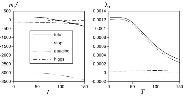
Figure 1: $\left(m_{3}^{2}\right)_{\rm eff}$ and $\lambda_{5}$ as functions of temperature $T$. The total values are given by the solid curves, the corrections from the stop, chargino-neutralino and the charged Higgs bosons are depicted by the dashed, dotted and dotted-dashed curves, respectively. For $T<T_{\rm low}=71.4$ the Higgs contributions are ignored.

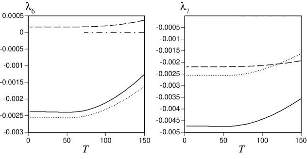
Figure 2: $\lambda_{6}$ and $\lambda_{7}$ as functions of temperature.

In this case, we have

$$B_{2}/T=1.532346\times 10^{-5},\qquad C_{1}/T=-4.846485\times 10^{-3}.$$ (4.5)

As seen from the curves in Fig. 2, $\lambda_{6,7}=O(10^{-3})$ so that $C_{1}\rho_{2}$ is comparable to $\lambda_{6}\rho_{1}^{2}+\lambda_{7}\rho_{2}^{2}$ for $\rho_{i}\sim 100$ at $T\simeq 100$. Hence, when $\left|G(\rho_{1},\rho_{2})\right|<1$, $\left(m_{3}^{2}\right)_{\rm eff}$ can be larger compared to the case of spontaneous $CP$ violation at $T=0$ if $C_{1}$ has the same sign as it, which is the present case. From (3.45), $C_{1}$ has the opposite sign to $\mu A_{t}$. At $T=100$, $\lambda_{5}=6.11026351\times 10^{-4}$ so that $F(\rho_{1},\rho_{2})>0$ for $\rho_{2}>4B_{2}/\lambda_{5}=10.03$. $\left|G(\rho_{1},\rho_{2})\right|$ is plotted for $T=70$, $75$, $80$ and $85$. There exists a region where the condition $\left|G(\rho_{1},\rho_{2})\right|<1$ is satisfied, as shown in Figs. 3 and 4 at each temperature.

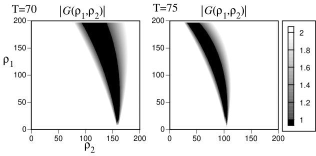
Figure 3: Contour plots of $\left|G(\rho_{1},\rho_{2})\right|$ at $T=70$ and $75$. $\left|G(\rho_{1},\rho_{2})\right|$ is satisfied in the black region.

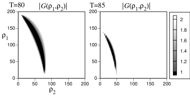
Figure 4: The same as Fig. 3 at $T=80$ and $85$.

(2) $\tan\beta_{0}=5$
Now $T_{\rm low}=312.48$, so that we ignore the charged Higgs contributions. The behaviors of the effective parameters are qualitatively the same as the example above, as depicted in Figs. 5 and 6. Tthe contributions from the charginos and neutralinos are identical to those above as obvious from (LABEL:eq:m32-gaugino) – (3.16).

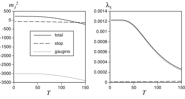
Figure 5: $\left(m_{3}^{2}\right)_{\rm eff}$ and $\lambda_{5}$ as functions of temperature. The total values are given by the solid curves, the corrections from the stop and chargino-neutralino are depicted by the dashed and dotted curves, respectively.

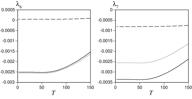
Figure 6: $\lambda_{6}$ and $\lambda_{7}$ as functions of temperature.

The larger $\tan\beta_{0}$ implies the smaller $y_{t}$ for a fixed $m_{t}$, that is, the smaller $\left|\Delta_{\tilde{t}}m_{3}^{2}(0)\right|$, which implies the larger $\left(m_{3}^{2}\right)_{\rm eff}$ for $\mu A_{t}>0$. This lowers the temperature at which $\left|G(\rho_{1},\rho_{2})\right|<1$ is satisfied for some $(\rho_{1},\rho_{2})$. In this case, we have

$$B_{2}/T=7.368276\times 10^{-6},\qquad C_{1}/T=-2.313638\times 10^{-3},$$ (4.6)

which implies $F(\rho_{1},\rho_{2})>0$ for $\rho_{2}>5.104$ at $T=100$, that is, $F(\rho_{1},\rho_{2})>0$ holds in the whole region in which $\left|G(\rho_{1},\rho_{2})\right|<1$ as shown in Figs. 7 and 8.

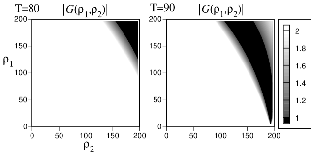
Figure 7: Contour plots of $\left|G(\rho_{1},\rho_{2})\right|$ at $T=80$ and $90$. $\left|G(\rho_{1},\rho_{2})\right|$ is satisfied in the black region.

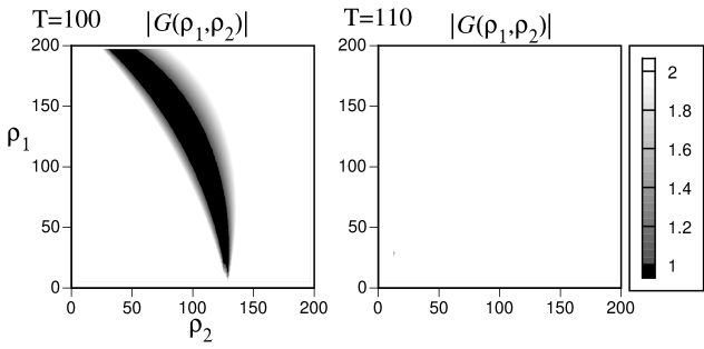
Figure 8: The same as Fig. 7 at $T=100$ and $110$.

(ii) $\mu A_{t}<0$
Although the stop contributions change their signs, those from the charginos and neutralinos are still dominant for the parameters in Table 2. This makes the temperature dependences of all the effective parameters milder than those in the case of $\mu A_{t}>0$. That is, for a wider range of temperature, the conditions for the spontaneous $CP$ violation will be satisfied.

lh

Table 2: The parameters used in the numerical analysis in the case of $\mu A_{t}<0$.

$m_{3}^{2}$	$A_{t}$	$M_{2}$	$\mu$	$m_{\tilde{q}}$
$2200$	$10$	$300$	$-300$	$400$

(1) $\tan\beta_{0}=1.2$
For this, $T_{\rm low}=75.313$, below which the Higgs contributions are neglected. The effective parameters are plotted in Figs. 9 and 10.

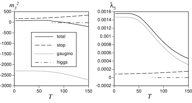
Figure 9: $\left(m_{3}^{2}\right)_{\rm eff}$ and $\lambda_{5}$ as functions of temperature $T$. The total values are given by the solid curves, the corrections from the stop, chargino-neutralino and the charged Higgs bosons are depicted by the dashed, dotted and dotted-dashed curves, respectively. For $T<T_{\rm low}=75.3$ the Higgs contributions are ignored.

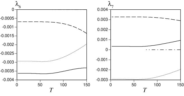
Figure 10: $\lambda_{6}$ and $\lambda_{7}$ as functions of temperature.

Since

$$B_{2}/T=3.447779\times 10^{-5},\qquad C_{1}/T=7.269727\times 10^{-3},$$ (4.7)

$F(\rho_{1},\rho_{2})>0$ for $\rho_{2}>16.05$ at $T=100$. The almost whole region where $\left|G(\rho_{1},\rho_{2})\right|<1$ satisfies this condition as well, as shown in Figs. 11 and 12. The positive $C_{1}$ requires smaller $m_{3}^{2}$ than that for $C_{1}<0$ to make $2\left(m_{3}^{2}\right)_{\rm eff}+2C_{1}\rho_{2}$ nearly equal to $\lambda_{6}\rho_{1}^{2}+\lambda_{7}\rho_{2}^{2}$.

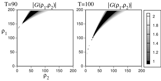
Figure 11: Contour plots of $\left|G(\rho_{1},\rho_{2})\right|$ at $T=90$ and $100$. $\left|G(\rho_{1},\rho_{2})\right|$ is satisfied in the black region.

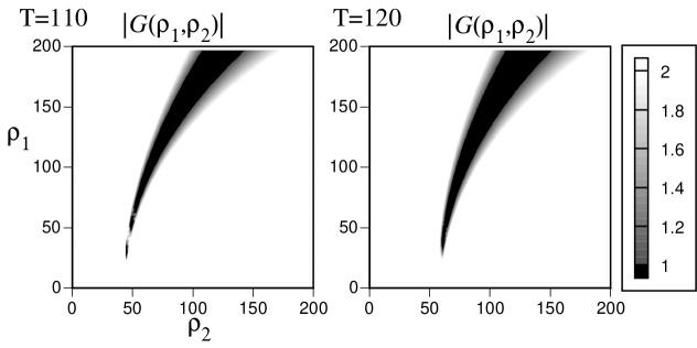
Figure 12: The same as Fig. 11 at $T=110$ and $120$.

(2) $\tan\beta_{0}=5$
Now $T_{\rm low}=313.08$. We completely ignore the Higgs contributions in the plots of the effective parameters in Figs. 13 and 14.

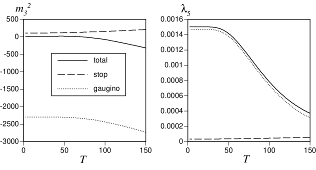
Figure 13: $\left(m_{3}^{2}\right)_{\rm eff}$ and $\lambda_{5}$ as functions of temperature. The total values are given by the solid curves, the corrections from the stop and chargino-neutralino are depicted by the dashed and dotted curves, respectively.

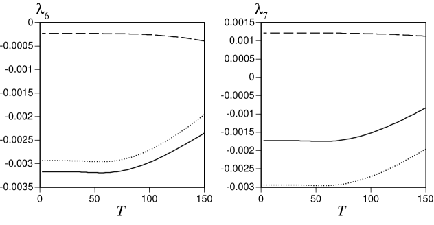
Figure 14: $\lambda_{6}$ and $\lambda_{7}$ as functions of temperature.

By the same reasoning as in the case of $\mu A_{t}>0$, the temperature at which $\left|G(\rho_{1},\rho_{2})\right|<1$ is lowered. At the same time, $\lambda_{5}$ becomes larger at lower temperatures so that the region with $\left|G(\rho_{1},\rho_{2})\right|<1$ grows as seen from Figs. 15 and 16. For this parameter set, we have

$$B_{2}/T=1.657862\times 10^{-5},\qquad C_{1}/T=3.470457\times 10^{-3},$$ (4.8)

which implies $F(\rho_{1},\rho_{2})>0$ for $\rho_{2}>8.463$ at $T=100$.

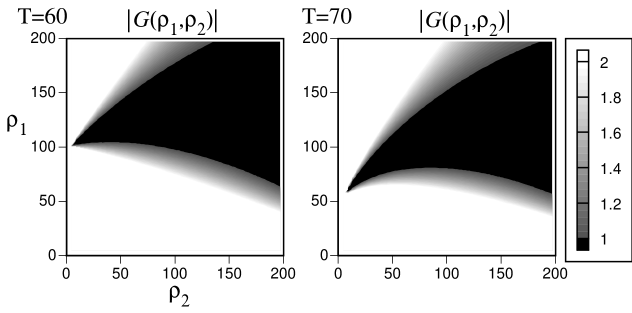
Figure 15: Contour plots of $\left|G(\rho_{1},\rho_{2})\right|$ at $T=60$ and $70$. $\left|G(\rho_{1},\rho_{2})\right|$ is satisfied in the black region.

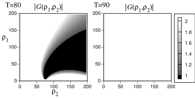
Figure 16: The same as Fig. 15 at $T=80$ and $90$.

5 Discussions

We have investigated the possibility of the new type of spontaneous $CP$ violation, which occurs at finite temperature in the transient region from the symmetric phase to the broken phase separated by the electroweak bubble wall. Since this type of $CP$ violation disappears in the broken phase at zero temperature, it is free from any constraint on $CP$ violation from the experiments. Further it will enhance the generated baryon number by the electroweak baryogenesis mechanism. Although the $CP$-conjugated pair of the bubbles degenerate in their energies as well as their nucleation rates, a tiny explicit $CP$ violation consistent with the observation such as the neutron EDM is sufficient to resolve the degeneracy and to leave the present BAU[9].

For this mechanism to work, some constraints are imposed on the parameters in the MSSM. First of all, $\mu M_{2}<0$ is required to make $\left(m_{3}^{2}\right)_{\rm eff}$ decrease by the chargino and neutralino contributions as noted in the previous section. $\left|\mu\right|\sim\left|M_{2}\right|$ yields a positive correction to $\lambda_{5}$ by these particles up to $T\simeq 100\mbox{GeV}$. For the expansion used for the light stop contributions to be valid, $\mu^{2}<m_{\tilde{q}}^{2}$ and $A_{t}^{2}<m_{\tilde{q}}^{2}$ are required. Together with $\left|\mu\right|\sim\left|M_{2}\right|$, these conditions make the stop contributions smaller than those from the charginos and neutralinos. The $\theta$-dependent $\rho^{3}$-terms are induced only if one of the soft-supersymmetry-breaking masses of the stop almost vanishes; $m_{\tilde{t}}\simeq 0$. Among the coefficients of these terms, $C_{1}$ gives contributions to the numerator of $G(\rho_{1},\rho_{2})$ comparable to those from the charginos and neutralinos. Whether $\left|G(\rho_{1},\rho_{2})\right|<1$ is satisfied is sensitive to $\left(m_{3}^{2}\right)_{\rm eff}$ in its numerator. Since $2C_{1}\rho_{2}$ appears in the numerator with the same sign as $\left(m_{3}^{2}\right)_{\rm eff}$, the effect of positive $C_{1}$ ($\mu A_{t}<0$) is compensated by reducing the tree-level $m_{3}^{2}$ as shown in the two examples in the previous section.

One might wonder how the difficulty encountered in the case of the spontaneous $CP$ violation at zero temperature[13] is avoided. $\lambda_{5}>0$ is satisfied at $T=0$ if the chargino and neutralino contributions dominate over those from the Higgs bosons and stops. This also applies to $F(\rho_{1},\rho_{2})$ in our case, except for the Higgs boson contribution, which is small since the effective $m_{1}^{2}m_{2}^{2}$ is larger than $m_{3}^{4}$ at $T\simeq T_{C}$. The problem was that for $\left|G(\rho_{1},\rho_{2})\right|<1$ to be satisfied at $T=0$, where $B_{1,2}=C_{1,2}=0$, $\left(m_{3}^{2}\right)_{\rm eff}$ must be so small as $(\lambda_{6}\cos^{2}\beta+\lambda_{7}\sin^{2}\beta)v_{0}^{2}$, which implies that the pseudoscalar boson is too light. Its mass $m_{A}$ is related to $m_{3}^{2}$ at the tree level by $m_{A}^{2}=(\tan\beta_{0}+\cot\beta_{0})m_{3}^{2}$. The smallest value of this tree-level $m_{A}$ in our examples is $m_{A}=67\mbox{GeV}$ for $m_{3}^{2}=2200\mbox{GeV}^{2}$ and $\tan\beta_{0}=1.2$. However, $m_{A}$ should be calculated at the minimum of the corrected potential. The value of $m_{A}$ calculated in this way might be sufficiently large for suitable range of the parameters. Further the parameters of the theory are not so constrained in our case compared to the case at $T=0$. This is because, if only the conditions are satisfied at some $(\rho_{1},\rho_{2})$ in the transient region, the $CP$ phase could be large enough to generate the BAU around the bubble wall.

Finally we emphasize that the spontaneously-$CP$-breaking minimum does not have to be the global minimum of $V_{\rm eff}$. The transitional $CP$ violation could take place if the conditions are satisfied for some fixed $(\rho_{1},\rho_{2})$, since such a bubble wall with transitional $CP$ violation would have a lower energy than that without $CP$ violation. Hence we do not need to be afraid that such a local minimum may not be the absolute minimum. For another reason, however, we should understand the global structure of the effective potential, which determines $T_{C}$, to know whether the transitional $CP$ violation occurs or not. In this sense, the conditions we examined here should be regarded as the necessary conditions but not the sufficient ones. With the knowledge of the global structure of $V_{\rm eff}$, one could find the $CP$-violating profile of the bubble wall so that one could estimate the generated baryon number.

Appendix A Loop Corrections

Here we summarize the expressions for the contributions to the effective parameters in terms of the finite-temperature Feynman integrals from the charginos, neutralinos, charged Higgs bosons and stops at finite temperature. We also show various formulas to calculate the Feynman integrals. According to the definitions of the effective parameters (3.8) – (3.11), the contribution of each particle is expressed in terms of the propagators in the symmetric phase ($\rho_{i}=0$) and the vertices which are related to the derivatives of the mass matrices.

The contributions from the charginos whose mass matrix is given by (3.12) to the effective parameters are

$$\Delta_{\chi^{\pm}}m_{3}^{2} = 2g_{2}^{2}\mu M_{2}\,i\int_{k}^{(+)}\Delta_{1}(k)\Delta_{2}(k),$$ (A.1)

$$\Delta_{\chi^{\pm}}\lambda_{5} = -2g_{2}^{4}(\mu M_{2})^{2}\,i\int_{k}^{(+)}\Delta_{1}^{2}(k)\Delta_{2}^{2}(k),$$ (A.2)

$$\Delta_{\chi^{\pm}}\lambda_{6} = \Delta_{\chi^{\pm}}\lambda_{7}=2g_{2}^{4}\mu M_{2}\,i\int_{k}^{(+)}k^{2}\Delta_{1}^{2}(k)\Delta_{2}^{2}(k),$$ (A.3)

where

$$\Delta_{1}(k)={1\over{k^{2}-M_{2}^{2}}},\qquad\Delta_{2}(k)={1\over{k^{2}-\mu^{2}}},$$ (A.4)

and the integral implies

$$\int_{k}^{(\mp)}\equiv iT\sum_{n=-\infty}^{\infty}\int{{d^{3}\mbox{\bf k}}\over{(2\pi)^{3}}}\quad\mbox{with }\left\{\begin{array}[]{ll}k_{0}=i\omega_{n}=2ni\pi/T&\mbox{for bosons}\\ k_{0}=i\omega_{n}=(2n+1)i\pi/T&\mbox{for fermions}.\end{array}\right.$$ (A.5)

The neutralino contributions are rather lengthy because of its mass matrix given by (3.13):

$$\Delta_{\chi^{0}}m_{3}^{2} = 2(g_{2}^{2}+g_{1}^{2})\mu\,i\int_{k}^{(+)}\Delta_{1}(k)\Delta_{2}(k)\Delta_{3}(k)\left[(k^{2}-P^{2})Q^{2}+PR^{2}\right],$$ (A.6)

$$\Delta_{\chi^{0}}\lambda_{5} = -4(g_{2}^{2}+g_{1}^{2})^{2}\mu^{2}\,i\int_{k}^{(+)}\Delta_{1}^{2}(k)\Delta_{2}^{2}(k)\Delta_{3}^{2}(k)(k^{2}-P^{2}-R^{2})$$ (A.7)

$${}\times\left[(k^{2}-P^{2})Q^{2}+PQR^{2}\right],$$

$$\Delta_{\chi^{0}}\lambda_{6} = \Delta_{\chi^{0}}\lambda_{7}=2(g_{2}^{2}+g_{1}^{2})\mu\,i\int_{k}^{(+)}\Delta_{1}^{2}(k)\Delta_{2}^{2}(k)\Delta_{3}^{2}(k)k^{2}(k^{2}-P^{2}-R^{2})$$ (A.8)

$${}\times\left[(2k^{2}-2P^{2}-R^{2})Q+PR^{2}\right],$$

where

$$\Delta_{1}(k) = {1\over{k^{2}-\mu_{1}^{2}}},\quad\Delta_{2}(k)={1\over{k^{2}-\mu_{2}^{2}}},\quad\Delta_{3}(k)={1\over{k^{2}-\mu^{2}}},$$ (A.9)

$$\mu^{2}_{1,2} = {{P^{2}+Q^{2}+2R^{2}\pm\left|P+Q\right|\sqrt{(P-Q)^{2}+4R^{2}}}\over 2},$$ (A.10)

with

$$P = M_{2}\sin^{2}\theta_{W}+M_{1}\cos^{2}\theta_{W},$$ (A.11)

$$Q = M_{2}\cos^{2}\theta_{W}+M_{1}\sin^{2}\theta_{W},$$ (A.12)

$$R = (M_{2}-M_{1})\sin\theta_{W}\cos\theta_{W}.$$ (A.13)

If $M_{1}=M_{2}$, $P=Q=M_{2}$ and $R=0$ so that $\mu_{1}=\mu_{2}=M_{2}$. In this case the neutralino contributions are reduced to

$$\Delta_{\chi^{0}}m_{3}^{2} = {1\over{\cos^{2}\theta_{W}}}\Delta_{\chi^{\pm}}m_{3}^{2},$$ (A.14)

$$\Delta_{\chi^{0}}\lambda_{5} = {2\over{\cos^{4}\theta_{W}}}\Delta_{\chi^{\pm}}\lambda_{5},$$ (A.15)

$$\Delta_{\chi^{0}}\lambda_{6} = \Delta_{\chi^{0}}\lambda_{7}={2\over{\cos^{4}\theta_{W}}}\Delta_{\chi^{\pm}}\lambda_{6}={2\over{\cos^{4}\theta_{W}}}\Delta_{\chi^{\pm}}\lambda_{7}.$$ (A.16)

We consider this special case of $M_{2}=M_{1}$ for simplicity.

The corrections to the effective parameters from the charged Higgs bosons are

$$\Delta_{\phi^{\pm}}m_{3}^{2} = -{1\over 2}g_{2}^{2}m_{3}^{2}\,i\int_{k}^{(-)}\Delta_{1}(k)\Delta_{2}(k),$$ (A.17)

$$\Delta_{\phi^{\pm}}\lambda_{5} = {1\over 4}g_{2}^{4}(m_{3}^{2})^{2}\,i\int_{k}^{(-)}\Delta_{1}^{2}(k)\Delta_{2}^{2}(k),$$ (A.18)

$$\Delta_{\phi^{\pm}}\lambda_{6} = -{1\over 4}g_{2}^{4}m_{3}^{2}\,i\int_{k}^{(-)}\Delta_{1}^{2}(k)\Delta_{2}^{2}(k)$$ (A.19)

$${}\times\left[k^{2}-{{m_{1}^{2}}\over{2\cos^{2}\theta_{W}}}-\left(1-{1\over{2\cos^{2}\theta_{W}}}\right)m_{2}^{2}\right],$$

$$\Delta_{\phi^{\pm}}\lambda_{7} = -{1\over 4}g_{2}^{4}m_{3}^{2}\,i\int_{k}^{(-)}\Delta_{1}^{2}(k)\Delta_{2}^{2}(k)$$ (A.20)

$${}\times\left[k^{2}-\left(1-{1\over{2\cos^{2}\theta_{W}}}\right)m_{1}^{2}-{{m_{2}^{2}}\over{2\cos^{2}\theta_{W}}}\right],$$

where

$$\Delta_{i}(k) = {1\over{k^{2}-\mu_{i}^{2}}},$$ (A.21)

$$\mu_{1,2}^{2} = {{m_{1}^{2}+m_{2}^{2}\pm\sqrt{(m_{1}^{2}-m_{2}^{2})^{2}+4m_{3}^{4}}}\over 2}.$$ (A.22)

In practice, we use the daisy-corrected ${\bar{m}}_{1,2}^{2}$ defined by (3.18) instead of $m_{1,2}^{2}$.

For the stop with $m_{\tilde{t}}=0$, we should treat the finite-temperature corrections from the heavy and light mass eigenstates separately. When $m_{\tilde{t}}\not=0$, the stop contributions are given by the integrals below.

$$\Delta_{\tilde{t}}m_{3}^{2} = -N_{c}y_{t}^{2}\mu A_{t}\,i\int_{k}^{(-)}\Delta_{1}(k)\Delta_{2}(k),$$ (A.23)

$$\Delta_{\tilde{t}}\lambda_{5} = N_{c}y_{t}^{4}(\mu A_{t})^{2}\,i\int_{k}^{(-)}\Delta_{1}^{2}(k)\Delta_{2}^{2}(k),$$ (A.24)

$$\Delta_{\tilde{t}}\lambda_{6} = -N_{c}y_{t}^{2}\mu A_{t}\,i\int_{k}^{(-)}\Bigl{[}-{1\over 4}\left({{g_{1}^{2}}\over 3}-g_{2}^{2}\right)\Delta_{1}^{2}(k)\Delta_{2}(k)$$ (A.25)

$${}+{{g_{1}^{2}}\over 3}\Delta_{1}(k)\Delta_{2}^{2}(k)+y_{t}^{2}\mu^{2}\Delta_{1}^{2}(k)\Delta_{2}^{2}(k)\Bigr{]},$$

$$\Delta_{\tilde{t}}\lambda_{7} = -N_{c}y_{t}^{2}\mu A_{t}\,i\int_{k}^{(-)}\Bigl{[}\left({1\over 4}\left({{g_{1}^{2}}\over 3}-g_{2}^{2}\right)+y_{t}^{2}\right)\Delta_{1}^{2}(k)\Delta_{2}(k)$$ (A.26)

$${}+\left(-{{g_{1}^{2}}\over 3}+y_{t}^{2}\right)\Delta_{1}(k)\Delta_{2}^{2}(k)+y_{t}^{2}A_{t}^{2}\Delta_{1}^{2}(k)\Delta_{2}^{2}(k)\Bigr{]},$$

where

$$\Delta_{1}(k)={1\over{k^{2}-m_{\tilde{q}}^{2}}},\qquad\Delta_{2}(k)={1\over{k^{2}-m_{\tilde{t}}^{2}}}.$$ (A.27)

The zero-temperature corrections can also be extracted from these integrals by use of the formulas given below. For $m_{\tilde{t}}^{2}=0$, we need the infrared cutoff to regularize the zero-temperature integrals to obtain the results (3.39) – (3.42). The finite-temperature Feynman integrals can be divided into the zero-temperature ones and the finite-temperature correction to them, which are usually expressed in terms of one-dimensional integrals. The integral appearing in the corrections to $m_{3}^{2}$ is simplified by the formula

$$-i\int_{k}^{(\mp)}\Delta_{1}(k)\Delta_{2}(k) = \int{{d^{4}k_{E}}\over{(2\pi)^{4}}}{1\over{(k^{2}+m_{1}^{2})(k^{2}+m_{2}^{2})}}\pm{1\over{2\pi^{2}}}f_{2}^{(\mp)}\!\left({m_{1}\over T},{m_{2}\over T}\right)$$ (A.28)

$$= L(m_{1},m_{2})\pm{1\over{2\pi^{2}}}f_{2}^{(\mp)}\!\left({m_{1}\over T},{m_{2}\over T}\right),$$

where the zero-temperature part is explicitly evaluated to yield

$$L(m_{1},m_{2})={1\over{16\pi^{2}}}\left[1-{m_{1}^{2}\over{m_{1}^{2}-m_{2}^{2}}}\log{m_{1}^{2}\over{M_{\rm ren}^{2}}}+{m_{2}^{2}\over{m_{1}^{2}-m_{2}^{2}}}\log{m_{2}^{2}\over{M_{\rm ren}^{2}}}\right]>0,$$ (A.29)

which is renormalized by the $\overline{\rm DR}$-scheme just as (3.6). $f_{2}^{(\mp)}(a,b)$ in the finite-temperature part is given by

$$f_{2}^{(\mp)}(a,b) = -{1\over{a^{2}-b^{2}}}\int_{0}^{\infty}dx\Bigl{(}{{x^{2}}\over\sqrt{x^{2}+a^{2}}}{1\over{e^{\sqrt{x^{2}+a^{2}}}\mp 1}}-{{x^{2}}\over\sqrt{x^{2}+b^{2}}}{1\over{e^{\sqrt{x^{2}+b^{2}}}\mp 1}}\Bigr{)},$$

for $a\not=b$ and

$$f_{2}^{(\mp)}(a,a)={1\over 2}\int_{0}^{\infty}{1\over{\sqrt{x^{2}+a^{2}}}}{1\over{e^{\sqrt{x^{2}+a^{2}}}\mp 1}}.$$ (A.31)

$f_{2}^{(\mp)}(a,b)$ is positive for any $(a,b)$.

The integrals in the corrections to $\lambda_{6,7}$ are calculated by use of the following integral:

$$-i\int_{k}^{(\mp)}\Delta_{1}^{2}(k)\Delta_{2}(k)={1\over{16\pi^{2}m_{1}^{2}}}H\left({{m_{1}^{2}}\over{m_{2}^{2}}}\right)\pm{1\over{2\pi^{2}T^{2}}}f_{3}^{(\mp)}\!\left({m_{1}\over T},{m_{2}\over T}\right),$$ (A.32)

where

$$H(\alpha)={\alpha\over{\alpha-1}}\left({1\over{\alpha-1}}\log\alpha-1\right),$$ (A.33)

with $H(1)=-1/2$ and

$$f_{3}^{(\mp)}(a,b)={1\over{2(a^{2}-b^{2})}}\int_{0}^{\infty}{{dx}\over{\sqrt{x^{2}+a^{2}}}}{1\over{e^{\sqrt{x^{2}+a^{2}}}\mp 1}}-{1\over{a^{2}-b^{2}}}f_{2}^{(\mp)}(a,b),$$ (A.34)

for $a\not=b$ and

$$f_{3}^{(\mp)}(a,a) = -{1\over 8}\int_{0}^{\infty}dx\Biggl{[}{1\over{(x^{2}+a^{2})^{3/2}}}{1\over{e^{\sqrt{x^{2}+a^{2}}}\mp 1}}+{1\over{x^{2}+a^{2}}}{{e^{\sqrt{x^{2}+a^{2}}}}\over{(e^{\sqrt{x^{2}+a^{2}}}\mp 1)^{2}}}\Biggr{]}.$$ (A.35)

$f_{3}^{(\mp)}(a,b)$ is negative for any $(a,b)$.

The integral in the corrections to $\lambda_{5}$ is reduced to

$$-i\int_{k}^{(\mp)}\Delta_{1}^{2}(k)\Delta_{2}^{2}(k)={1\over{16\pi^{2}m_{1}^{4}}}K\left({{m_{1}^{2}}\over{m_{2}^{2}}}\right)\pm{1\over{2\pi^{2}T^{4}}}f_{4}^{(\mp)}\!\left({m_{1}\over T},{m_{2}\over T}\right),$$ (A.36)

where

$$K(\alpha)={\alpha\over{(\alpha-1)^{2}}}\left({{\alpha+1}\over{\alpha-1}}\log\alpha-2\right),$$ (A.37)

with $K(1)=1/6$ and

$$f_{4}^{(\mp)}(a,b) = {1\over{2(a^{2}-b^{2})^{2}}}\int_{0}^{\infty}dx\Bigl{(}{1\over{\sqrt{x^{2}+a^{2}}}}{1\over{e^{\sqrt{x^{2}+a^{2}}}\mp 1}}$$ (A.38)

$$\qquad+{1\over{\sqrt{x^{2}+b^{2}}}}{1\over{e^{\sqrt{x^{2}+b^{2}}}\mp 1}}\Bigr{)}-{2\over{(a^{2}-b^{2})^{2}}}f_{2}^{(\mp)}(a,b),$$

for $a\not=b$ and

$$f_{4}^{(\mp)}(a,a) = {1\over{16}}\int_{0}^{\infty}dx\Biggl{\{}{1\over{(x^{2}+a^{2})^{5/2}}}{1\over{e^{\sqrt{x^{2}+a^{2}}}\mp 1}}+\Bigl{[}{1\over{(x^{2}+a^{2})^{2}}}$$ (A.39)

$$\qquad\qquad-{1\over{3(x^{2}+a^{2})^{3/2}}}\Bigr{]}{{e^{\sqrt{x^{2}+a^{2}}}}\over{(e^{\sqrt{x^{2}+a^{2}}}\mp 1)^{2}}}$$

$$\qquad\qquad+{2\over{3(x^{2}+a^{2})^{3/2}}}{{e^{2\sqrt{x^{2}+a^{2}}}}\over{(e^{\sqrt{x^{2}+a^{2}}}\mp 1)^{3}}}\Biggr{\}}.$$

$f_{4}^{(\mp)}(a,b)$ is positive for any $(a,b)$.

References

[1] For a review see, A. Cohen, D. Kaplan and A. Nelson,
Ann. Rev. Nucl. Part. Sci. 43 (1993) 27.
K. Funakubo,Prog. Theor. Phys. 96 (1996) 475.
[2] M. Carena, M. Quiros, C.E.M. Wagner, Phys. Lett. B380 (1996) 81.
[3] D. Delepine, J.-M. Gerard, R. Gonzalez Felipe, J. Weyers,
Phys. Lett. B386 (1996) 183.
[4] P. Huet and A. Nelson, Phys. Rev. D53 (1996) 4578.
M. Aoki, N .Oshimo and A. Sugamoto, Prog. Theor. Phys. 98 (1997) 1179.
M. P. Worah, Phys. Rev. Lett. 79 (1997) 3810.
[5] A. Nelson, D. Kaplan and A. Cohen, Nucl. Phys. B373 (1992) 453.
[6] K. Funakubo, A. Kakuto, S. Otsuki, K. Takenaga and F. Toyoda,
Phys. Rev. D50 (1994) 1105.
[7] K. Funakubo, A. Kakuto, S. Otsuki, K. Takenaga and F. Toyoda,
Prog. Theor. Phys. 94 (1995) 845.
[8] K. Funakubo, A. Kakuto, S. Otsuki, K. Takenaga and F. Toyoda,
Prog. Theor. Phys. 93 (1995) 1067.
[9] K. Funakubo, A. Kakuto, S. Otsuki and F. Toyoda,
Prog. Theor. Phys. 96 (1996) 771.
[10] K. Funakubo, A. Kakuto, S. Otsuki, F. Toyoda,
Prog. Theor. Phys. 98 (1997) 427.
[11] D. Comelli, M. Pietroni and A. Riotto, Nucl. Phys. B412 (1994) 441.
[12] J.R. Espinosa, J.M. Moreno and M. Quiros, Phys. Lett. B324 (1994) 181.
[13] N. Maekawa, Phys. Lett. B282 (1992) 387;
Nucl. Phys. Suppl. 37A (1994) 191.
[14] L. Dolan and R. Jackiw, Phys. Rev. D9 (1974) 3320.
[15] S. Coleman and E. Weinberg, Phys. Rev. D7 (1973) 1888.