Field Strength Correlators and Dual Effective Dynamics in QCD

Abstract

We establish a relation between the two-point field strength correlator in QCD and the dual field propagator of an effective dual Abelian Higgs model describing the infrared behaviour of QCD. We find an analytic approximation to the dual field propagator without sources and in presence of quark sources. In the latter situation we also obtain an expression for the static $q\bar{q}$ potential. Our derivation sheds some light on the dominance and phenomenological relevance of the two-point field strength correlator.

I INTRODUCTION

The gauge invariant field strength vacuum correlators

$$\langle F_{\mu_{1}\nu_{1}}(x_{1})U(x_{1},x_{2})F_{\mu_{2}\nu_{2}}(x_{2})U(x_{2},x_{3})\cdots F_{\mu_{n}\nu_{n}}(x_{n})U(x_{n},x_{1})\rangle,$$ (1)

where $U(x,y)\equiv{\rm P}\displaystyle\exp ig\int_{y}^{x}dz^{\mu}A_{\mu}(z)$ is the Schwinger color string, play a relevant role in gluodynamics with and without quark sources. We know that in the infrared region these correlators are dominated by their non-perturbative behaviour. In particular the non-perturbative “gluon condensate”

$$\langle{\alpha_{s}\over\pi}F_{\mu\nu}^{a}(0)F^{\mu\nu}_{a}(0)\rangle^{\rm non\,pert}\equiv F_{2},$$ (2)

plays a crucial role in the QCD sum rule method [1].

The non-perturbative part of the gauge invariant two-point field strength correlator $\langle F_{\mu\nu}(x)U(x,0)F_{\rho\sigma}(0)U(0,x)\rangle$ has been calculated on the lattice, with the cooling method in [2] and in presence of sources in [3]. We define (in Euclidean space-time, as in the rest of this work) the gauge invariant correlator [4]

$$\langle g^{2}F_{\mu\nu}(x)U(x,0)F_{\lambda\rho}(0)U(0,x)\rangle \equiv (\delta_{\mu\lambda}\delta_{\nu\rho}-\delta_{\mu\rho}\delta_{\nu\lambda})g^{2}D(x^{2})+{1\over 2}\left[{\partial\over\partial x_{\mu}}\left(x_{\lambda}\delta_{\nu\rho}-x_{\rho}\delta_{\nu\lambda}\right)\right.$$ (3)

$$+ \left.{\partial\over\partial x_{\nu}}\left(x_{\rho}\delta_{\mu\lambda}-x_{\lambda}\delta_{\mu\rho}\right)\right]g^{2}D_{1}(x^{2})\,.$$ (4)

A parameterization of the form

$$D(x^{2})=Ae^{-|x|/T_{g}}+{a\over x^{4}}e^{-|x|/T_{p}}\qquad D_{1}(x^{2})=Be^{-|x|/T_{g}}+{b\over x^{4}}e^{-|x|/T_{p}}$$ (5)

$$A\simeq 128~{}{\rm GeV}^{4},\qquad B\simeq 27~{}{\rm GeV}^{4},\qquad a\simeq 0.69,\qquad b\simeq 0.46,$$ (6)

$$T_{g}\simeq 0.22~{}{\rm fm},\qquad T_{p}\simeq 0.42~{}{\rm fm},$$ (7)

yields a very good fit to the (cooled) lattice data [2] in the range $0.1\,{\rm fm}\leq x\leq 1\,{\rm fm}$. At short distances the $1/x^{4}$ term, which is of perturbative origin, dominates, while at distances $x\geq 0.4\,{\rm fm}$ the non-perturbative term, proportional to $e^{-{x/T_{g}}}$, becomes more important. In an Abelian theory without monopoles the Bianchi identities yields $D=0$.

In the Stochastic Vacuum Model (SVM) [4, 5, 6, 7] it is assumed that for processes which can be reduced to the calculation of Wilson loops with quasi-static sources (such as heavy quark potentials and soft high energy scattering amplitudes in the eikonal approximation) the infrared behaviour of QCD can be approximated by a Gaussian stochastic process in the field strength and is thus determined approximately by the correlator (4). In particular also the Wilson loop average is given only in terms of (4).

We know from the strong coupling expansion and lattice simulations that the Wilson loop is an order parameter for confinement. The confining area law behaviour of the Wilson loop is reproduced by the stochastic vacuum model provided that the form factor $D$ is different from zero and is dominated in the infrared region by a decreasing behaviour with the fall off controlled by a finite correlation length $T_{g}$. These features of $D$ are compatible with lattice data (see (5)). Furthermore this model gives a good description of certain features of high energy scattering (e. g. [8]). We will come back to this point in Sec. 2.

It is the goal of this paper to relate the gluon correlator to the Mandelstam–’t Hooft dual superconductor mechanism of confinement [9]. In this picture the physical essence of the confinement is the formation of color-electric flux tubes between quarks due to a dual Meissner effect. The monopoles condense and lead to a dual superconductor which forces the color-electric field lines in flux tubes which are the dual analogue to the Abrikosov–Olesen strings. The formation of an electric flux tube is also the consequence of the Stochastic Vacuum Model [10].

Furthermore, in an Abelian projection of QCD, monopoles are the degrees of freedom responsible for confinement. Monopoles condensation has been observed on the lattice (for a review see [11]) and when confinement can be derived analytically (compact electrodynamics, Georgi–Glashow model, and some supersymmetric Yang–Mills theories), it is due to the condensation of monopoles. The monopole potential can be measured in the Abelian projection and it turns out that in the confining phase it has the Higgs form [12]. Lattice measurements of the distribution of monopole currents indicate that at large distances gluodynamics is equivalent to a dual Abelian Higgs model, the Higgs particles are Abelian monopoles and these are condensed in the confining phase. In the maximal Abelian gauge the structure of the interquark flux tube was intensively studied and high precision measurements of the colour fields and the monopole currents recently allowed for a detailed check of the dual superconductor scenario with respect to the Ginzburg–Landau equations [13].

Analytic models of the infrared dynamics of dual QCD with monopoles were constructed [14, 15] and their phenomenological consequences intensively investigated. In the effective dual model of Baker, Ball and Zachariasen (dual QCD, DQCD), the complete semirelativistic quark-antiquark potential, the flux tube distribution and the energy density were obtained from the numerical solution of the coupled non-linear equations of motion and compared very favourably with recent lattice data [16, 17, 18]. Although the Lagrangian of this effective dual theory for long distance QCD is based on a non-Abelian gauge group, the results for the $q\bar{q}$ potentials aside from an overall color factor can to a very good approximation be described by a (dual) Abelian Higgs model. Therefore, the results are in this case largely insensitive to the details of the dual gauge group and the quarks select out only Abelian configurations of the dual potential [19].

Since an effective Abelian description of the infrared confining dynamics of QCD (at least for heavy quarks) emerges either from QCD (via Gaussian approximation and bilocal strength tensor correlators) or via an effective Abelian Higgs models it becomes extremely interesting to exploit in which sense the two Abelian descriptions are equivalent and, once we assume an equivalence, what kind of constraints this imposes on the form of the QCD field strength correlators. In the present work we will obtain from the dual Abelian Higgs model information on the form of the gauge invariant two-point field strength correlator (4) and in addition we will obtain an analytic approximation for the static heavy quark potential given by the dual theory.

There are two more arguments which motivate such an investigation. First, as we will discuss briefly in Sec. 2, the existence of a non-vanishing form factor $D$ in the two-point field strength correlator of QCD seems to suggest quite naturally the existence of an effective free dual Abelian theory “behind” the long-range dynamics of QCD. Second, a recent comparison between the complete semirelativistic potentials obtained in DQCD and in the Gaussian stochastic approximation of QCD in the limit of large interquark distances showed up quite striking and surprising similarities (see [20]). The following analysis wants to shed some light on that.

The plan of the paper is the following. In Sec. 2 we recollect some essential features of the gauge invariant two-point correlator in QCD and we establish a relation with the Wilson loop. In Sec. 3 we investigate the analogous quantity in the dual Abelian Higgs model without sources. For a constant Higgs field we reproduce a two-point correlator having the same behaviour as obtained by other authors by studying the London limit of a dual Abelian Higgs model. In Sec. 4 we introduce sources and obtain an analytic expression for the static potential. This suggests a connection between the parameters of the two-point field strength correlator in QCD and those of the dual Abelian Higgs model. Finally, Sec. 5 contains some conclusions.

II GAUGE-INVARIANT TWO-POINT GLUON CORRELATOR AND WILSON LOOP IN QCD

We consider the correlator of two gluon field strengths in QCD at different space-time points, connected by a Schwinger string. This string can either consist of two strings in the fundamental representation or one string in the adjoint one. For definiteness in notation we choose the first possibility and consider the quantity

$$\langle g^{2}F_{\mu\nu}(x)\,U(x,0)F_{\lambda\rho}(0)U(0,x)\rangle.$$

The Lorentz decomposition of this correlator is given by Eq. (4) and the results of the lattice measurements are collected in Eq. (5). The leading (tree level) perturbative contribution is contained in the form factor $D_{1}$. In an Abelian gauge theory without monopoles the Bianchi identity implies that the form factor $D$ vanishes identically [4]. In a non-Abelian theory or in an Abelian theory with monopoles $D$ can be different from zero. Let us briefly review how a non-vanishing $D$ leads to confinement [4].

In the presence of heavy quark sources the relevant object in QCD is the Wilson loop average $W(\Gamma)$, where $\Gamma$ is a closed curve built up by the trajectories of external sources and some Schwinger strings connecting the end-points. By means of the non-Abelian Stokes theorem [21] one can express the Wilson loop average $W(\Gamma)$ in terms of an integral over a surface $S(\Gamma)$ enclosed by the contour $\Gamma$. A way to evaluate analytically this quantity consists in expanding this expression via a cluster expansion and keeping only the bilocal cluster (i. e. in assuming that the vacuum fluctuations are of a Gaussian type):

$$W(\Gamma) \equiv \left\langle{\rm P}\>\exp\left(ig\int_{\Gamma}dz_{\mu}A_{\mu}(z)\right)\right\rangle{\mathop{=}\limits_{{\rm Stokes}}}\left\langle{\rm P}\>\exp\left(ig\int_{S(\Gamma)}dS_{\mu\nu}(u)F_{\mu\nu}(u,x_{0})\right)\right\rangle$$ (8)

$${\mathop{\simeq}\limits_{{\rm SVM}}} \exp\left(-{1\over 2}\int_{S(\Gamma)}dS_{\mu\nu}(u)\int_{S(\Gamma)}dS_{\lambda\rho}(v)\langle g^{2}F_{\mu\nu}(u,x_{0})F_{\lambda\rho}(v,x_{0})\rangle\right),$$ (9)

where ${\rm P\,}F_{\mu\nu}(u,x_{0})\equiv{\rm P\,}U(u,x_{0})F_{\mu\nu}(u)U(x_{0},u)$. Assumption (9) corresponds to the so-called Stochastic Vacuum Model (SVM) [4]. The point $x_{0}$ is an arbitrary reference point on the surface $S(\Gamma)$ needed for surface ordering. Of course the final result in the full theory does not depend on the reference point $x_{0}$. The results obtained in the Gaussian approximation, however, will generally depend on it. This dependence is minimized by choosing $S(\Gamma)$ to be the minimal area surface with contour $\Gamma$ [22]. Under this condition one may neglect the $x_{0}$ dependence on $\langle g^{2}F_{\mu\nu}(u,x_{0})F_{\lambda\rho}(v,x_{0})\rangle$ and recover in this way translational invariance. Then, the decomposition of Eq. (4) can be used (by replacing $x^{2}$ with $(u-v)^{2}$).

All the spin and velocity dependent potentials up to order $1/m^{2}$ in the quark mass can be expressed in terms of the functions $D$ and $D_{1}$ [5, 20, 23]. In particular the static potential is given by

$$V_{0}(R)={g^{2}\over 2}\int_{|x_{1}|<R}d^{2}x~{}(R-|x_{1}|)~{}D(x^{2})+{|x_{1}|\over 2}D_{1}(x^{2}),$$ (10)

with $d^{2}x=dx_{1}dx_{4}$, $x^{2}=x_{1}^{2}+x_{4}^{2}$. The string tension emerges for large $q\bar{q}$ distances $R$ as

$$\sigma={g^{2}\over 2}\int d^{2}x\,D(x^{2}).$$ (11)

Therefore a non-vanishing $D$ function leads to confinement.

While lattice data confirm the existence of a non-vanishing form factor $D$ with exponential fall off, up to now there is no analytic tool which allows to calculate and to interpret the non-perturbative contributions to $D$ in the long-range regime.

We observe, however, that a non-vanishing function $D$ emerges naturally if we assume that there exists an effective “dual” Lagrangian describing an Abelian gauge theory for which the dual two-point field strength correlator coincides in the long-range limit with the bilocal cumulant given by Eq. (4). Let us call $G_{\mu\nu}$ the (Abelian) field strength of the dual theory. Since we assume this theory to observe the Bianchi identities we have in general

$$\langle g^{2}G_{\mu\nu}(x)G_{\lambda\rho}(0)\rangle\equiv{1\over 2}\left[{\partial\over\partial x_{\mu}}\left(x_{\lambda}\delta_{\nu\rho}-x_{\rho}\delta_{\nu\lambda}\right)+{\partial\over\partial x_{\nu}}\left(x_{\rho}\delta_{\mu\lambda}-x_{\lambda}\delta_{\mu\rho}\right)\right]g^{2}\Delta(x^{2}).$$

The expectation value of the dual of the dual fields, $\tilde{G}_{\mu\nu}\equiv\displaystyle{1\over 2}\epsilon_{\mu\nu\alpha\beta}G_{\alpha\beta}$, is

$$\langle g^{2}\tilde{G}_{\mu\nu}(x)\tilde{G}_{\lambda\rho}(0)\rangle = (\delta_{\mu\lambda}\delta_{\nu\rho}-\delta_{\mu\rho}\delta_{\nu\lambda})g^{2}\left(\Delta(x^{2})-x^{2}{d\over dx^{2}}\Delta(x^{2})\right)$$ (12)

$$+ 2\left[{\partial\over\partial x_{\mu}}\left(x_{\lambda}\delta_{\nu\rho}-x_{\rho}\delta_{\nu\lambda}\right)+{\partial\over\partial x_{\nu}}\left(x_{\rho}\delta_{\mu\lambda}-x_{\lambda}\delta_{\mu\rho}\right)\right]g^{2}{d\over dx^{2}}{d\over dx^{2}}\Delta(x^{2}).$$ (13)

It shows a tensor structure like the one multiplying $D$ in equation (4). The existence of such a correlator therefore seems to suggest the existence of a dual Abelian gauge theory for which at big distances the field strength correlator behaves as the corresponding correlator of the dual theory:

$$\langle g^{2}F_{\mu\nu}(x,x_{0})F_{\lambda\rho}(0,x_{0})\rangle\sim\langle g^{2}\tilde{G}_{\mu\nu}(x)\tilde{G}_{\lambda\rho}(0)\rangle.$$ (14)

In the next section we want to explore some consequences of Eq. (14). In Sec. 4 Eq. (14) will be replaced by a better founded assumption on the Wilson loop. Nevertheless the basic idea behind (14) will remain.

III DUAL ABELIAN HIGGS MODEL WITHOUT SOURCES OR VORTICES

The aim of this section is essentially pedagogical. We will reproduce in a clear and economical way some of the results which can be found in the existing literature on the London limit of a dual Abelian Higgs model. We will prove in this way that assumption (14) is reasonable, i. e. compatible with (5). We will also show the drawbacks of this approach and try to justify why we need to take into account external charge sources. This will lead to the results of Sec. 4.

Let us consider a very naive context, i. e. a “dual” vector gauge field $C_{\mu}$ minimally coupled with some external scalar field $\phi$ which we could call a Higgs field. The action is given by

$$S(C_{\mu},\phi)=\int d^{4}x\left[{1\over 4}G_{\mu\nu}(x)G_{\mu\nu}(x)+{1\over 2}(D_{\mu}\phi)^{*}(x)(D_{\mu}\phi)(x)+V(\phi^{*}(x)\phi(x))\right],$$ (15)

where $G_{\mu\nu}(x)=\partial_{\mu}C_{\nu}(x)-\partial_{\nu}C_{\mu}(x)$ and $V(\phi^{*}\phi)=\displaystyle{\lambda\over 4}(\phi^{*}\phi-\phi_{0}^{2})^{2}$ (with $\phi_{0}$ different from zero). The Higgs field is coupled to the gauge field $C_{\mu}$ via the covariant derivative $D_{\mu}\phi=(\partial_{\mu}+ieC_{\mu})\phi$.

We choose a gauge in which the regular part of the phase of $\phi$ vanishes, the so-called unitary gauge. The propagator, ${\cal K}_{\mu\nu}\equiv\langle C_{\mu}C_{\nu}\rangle$, of the field $C_{\mu}$ satisfies the equation:

$$(\partial^{2}\delta_{\nu\mu}-\partial_{\nu}\partial_{\mu}-e^{2}\phi^{2}(x)\delta_{\nu\mu}){\cal K}_{\nu\alpha}(x,y)=-\delta_{\mu\alpha}\delta^{4}(x-y).$$ (16)

The quantity in which we are interested is what we could call the “dual” of the field strength two-point correlator in the theory described by the action (15):

$${\cal G}_{\sigma\gamma\lambda\rho}(x,y)\equiv(\delta_{\lambda\sigma}\delta_{\rho\gamma}-\delta_{\lambda\gamma}\delta_{\rho\sigma})\delta^{4}(x-y)-\epsilon_{\mu\nu\lambda\rho}\epsilon_{\beta\alpha\sigma\gamma}\partial^{y}_{\beta}\partial^{x}_{\mu}{\cal K}_{\nu\alpha}(x,y).$$ (17)

For a matter of convenience we prefer to define ${\cal G}_{\sigma\gamma\lambda\rho}$ with the delta contribution subtracted out explicitly. In this model ${\cal G}_{\sigma\gamma\lambda\rho}$ is the equivalent of the quantity $\langle g^{2}\tilde{G}_{\mu\nu}(x)\tilde{G}_{\lambda\rho}(y)\rangle$ introduced at the end of the last Section. Eqs. (17) and (14) then give the correlator (4) in terms of the propagator of the dual theory.

Let us study, now, the case where the Higgs field has the constant value $\phi_{0}$. Then, Eq. (16) can be written as:

$$(\partial^{2}-e^{2}\phi_{0}^{2}){\cal K}^{\infty}_{\mu\alpha}(x,y)=-\left(\delta_{\mu\alpha}-{\partial_{\mu}\partial_{\alpha}\over e^{2}\phi_{0}^{2}}\right)\delta^{4}(x-y).$$ (18)

This is simply the equation defining the free propagator of a massive vector boson with mass $M\equiv e\phi_{0}$:

$${\cal K}^{\infty}_{\mu\alpha}(x,y) = \left(\delta_{\mu\alpha}-{\partial_{\mu}\partial_{\alpha}\over M^{2}}\right){\cal K}^{\infty}(x-y),$$ (19)

$$\hbox{with}\>{\cal K}^{\infty}(x-y) = \int{d^{4}p\over(2\pi)^{4}}e^{-ip(x-y)}{1\over p^{2}+M^{2}}={M\over(2\pi)^{2}}{K_{1}(Mx)\over x},$$ (20)

where $K_{n}$ ($n=0,1,2,\dots$) are Bessel functions. As a consequence we can write

$${\cal G}_{\sigma\gamma\lambda\rho}(x-y) = (\delta_{\lambda\sigma}\delta_{\rho\gamma}-\delta_{\lambda\gamma}\delta_{\rho\sigma})D^{\infty}((x-y)^{2})+{1\over 2}\left[{\partial\over\partial x_{\lambda}}\left((x-y)_{\sigma}\delta_{\rho\gamma}-(x-y)_{\gamma}\delta_{\rho\sigma}\right)\right.$$ (21)

$$+ \left.{\partial\over\partial x_{\rho}}\left((x-y)_{\gamma}\delta_{\lambda\sigma}-(x-y)_{\sigma}\delta_{\lambda\gamma}\right)\right]D^{\infty}_{1}((x-y)^{2}),$$ (22)

with

$$D^{\infty}(x^{2}) = \delta^{4}(x)+\partial^{2}{\cal K}^{\infty}(x^{2})=M^{2}{\cal K}^{\infty}(x^{2})={M^{3}\over 4\pi^{2}}{K_{1}(Mx)\over x},$$ (23)

$$D^{\infty}_{1}(x^{2}) = -4{d\over dx^{2}}{\cal K}^{\infty}(x^{2})={M\over 2\pi^{2}x^{2}}\left[{K_{1}(Mx)\over x}+{M\over 2}(K_{0}(Mx)+K_{2}(Mx))\right].$$ (24)

Therefore, the assumption that ${\cal G}_{\sigma\gamma\lambda\rho}$ has the same long-range behaviour of the gauge invariant two-point field strength correlator in QCD (see Eq. (14)) is compatible with the parameterization (5) and leads to a correlation length $T_{g}$ equal to the inverse of the dual gluon mass $M$. In particular, the asymptotic behaviours of ${\cal K}^{\infty}$ are:

$${\cal K}^{\infty}(x^{2}) {\mathop{\longrightarrow}\limits_{|x|\to 0}} {1\over(2\pi)^{2}}{1\over x^{2}}+\cdots,$$ (25)

$${\cal K}^{\infty}(x^{2}) {\mathop{\longrightarrow}\limits_{|x|\to\infty}} {1\over 2}{1\over(2\pi)^{3/2}}{1\over\sqrt{M}x^{3/2}}e^{-Mx}+\cdots.$$ (26)

The results shown here coincide with those obtained from the London limit of a dual Abelian Higgs model in [26]. The seeming difference for what concerns the function $D$ is due to the fact that we have subtracted out explicitly in our definition of ${\cal G}_{\sigma\gamma\lambda\rho}$ the delta singularity which in the referred work is taken into account in a regularized form. One may wonder how the result of a topologically trivial model (no singular Higgs phase) agrees with results which take into account properly the internal Abrikosov–Nielsen–Olesen strings. This is due to the fact that ${\cal G}_{\sigma\gamma\lambda\rho}$ is sensitive to the string only via the strength of the Higgs field and this is fixed to a constant here as well as in the London limit of a dual Abelian Higgs model.

The agreement between both approaches reveals a common weakness: the missing treatment of the interaction between the internal strings present in the dual Abelian Higgs model and the string between external quark sources. In Ref. [26] no external sources were introduced and the result (23)-(24) for the correlator was obtained in the following way. The functional integral for the Abelian Higgs model was rewritten in such a form as to exhibit integration over the closed surfaces of the (internal) strings. From the form of the contribution of a single closed surface in the London limit it was deduced that it could be obtained by a correlator like (23)-(24) in the Gaussian approximation. Implicitly this form was assumed to be valid also for external sources. When external quark sources are introduced however, the strings of those sources will interfere with the internal strings. Some aspects of that phenomenon (the linking number) have been treated in [27], but to our knowledge there exists no analytic attempt to evaluate the influence on the phenomenologically relevant parameters.

We notice that, due to the short-range behaviour (25), Eq. (24) reproduces the expected short-range behaviour of the function $D_{1}$ ($\sim 1/x^{4}$, see (5)). Due to the short distance behaviour of the function $D$, like $1/x^{2}$, the string tension we obtained using (14), Eq. (23) and Eq. (11), is logarithmically divergent:

$$\sigma^{\infty}\equiv{g^{2}\over 2}{\mathop{\lim}\limits_{\epsilon\to 0}}\int_{|x|>\epsilon}d^{2}x\,D^{\infty}(x^{2})=\pi\phi_{0}^{2}\,\,{\mathop{\lim}\limits_{\epsilon\to 0}}\,K_{0}(\epsilon)\sim\pi\phi_{0}^{2}\,(\log 2-\log\epsilon-\gamma),$$ (27)

where we have used the Dirac quantization condition $e=2\pi/g$, relating $g$ to the coupling constant $e$ of the dual theory. The divergence is a short-distance effect and appears to be a result of the freezing of the Higgs field to the vacuum value $\phi_{0}$, i. e., in terms of the dual Abelian Higgs model, of the London limit. Assuming a coordinate dependent Higgs mass going to zero like $|x|$ near the origin, would yield a finite short-range behaviour of the function $D^{\infty}$ while preserving the perturbative short-range behaviour of the function $D_{1}^{\infty}$. There is, however, no motivation for such an anisotropic behaviour of the Higgs field unless we introduce some charges into the vacuum. Only in such a context we can expect that near the sources and on the connecting flux tube string the Higgs field vanishes while far away it assumes the vacuum value $\phi_{0}$. This will be precisely the subject of the next section, where we will consider a dual Abelian Higgs model with external charges and where we will also change our intuitive duality assumption (14) to a more physically justified one. Moreover, we recall here that recent lattice data [13] confirm that in the presence of external quark sources the distribution of electric fields and monopoles currents does not fulfill the London limit.

To conclude this section we comment briefly on the translational invariance of the considered correlators. As long as $\phi$ is considered as an external field in Eq. (16), ${\cal G}_{\sigma\gamma\lambda\rho}$ is not translational invariant and therefore in order to take advantage of the decomposition (4) we have to fix our reference frame in such a way that the point $y$ coincides with the origin. This fact is by itself not in contradiction with the duality assumption (14) since also the correlator in the direct theory, $\langle F_{\mu\nu}(x,x_{0})F_{\lambda\rho}(y,x_{0})\rangle$, is in general not translational invariant, and only by choosing the reference point $x_{0}$ on the straight line connecting $x$ with $y$ is invariance recovered. Finally, we notice that ${\cal G}_{\sigma\gamma\lambda\rho}$ is translational invariant in some particular cases: if we assume $\phi$ constant, as we have done in this section, or partially (in the longitudinal coordinates) if we assume that $\phi$ depends only on some (transverse) coordinates. This last situation will be exploited in the next section.

IV DUAL ABELIAN HIGGS MODEL WITH EXTERNAL QUARK SOURCES

In this section, for the reasons stated above, we want to consider a dual Abelian Higgs model with external quark sources. In particular we want to make a duality assumption on the long-range behaviour of the Wilson loop associated with the dynamics of a two heavy quark bound state. This assumption will take the place of our previous statement (14). We will see that some general features will, nevertheless, be preserved.

Following [19] we assume that the long-range behaviour of the Wilson loop average $W(\Gamma)$ associated with a two heavy quark bound state is described by the functional generator of a dual Abelian Higgs model with external quark sources :

$$W(\Gamma)\sim\langle e^{-S(C_{\mu},\phi)}\rangle,$$ (28)

where the bracket $\langle~{}~{}\rangle$ means the average over the gauge fields $C_{\mu}$ and the Higgs field $\phi$. The Abelian Higgs model is dual in the sense that it is weakly coupled. Therefore the right-hand side of Eq. (28) can be evaluated via a classical expansion.

The action $S$ is given by equation (15), but since we want that in the $\lambda=0$ limit $S$ describes the dual of a $U(1)$ Yang–Mills theory with two external point-like charge sources $-g$ (particle) and $g$ (antiparticle), we define the field strength tensor $G_{\mu\nu}$, now, in such a way that it contains not only the dual gauge fields $C_{\mu}$ but also the field of the external sources [28]:

$$G_{\mu\nu}(x)=\partial_{\mu}C_{\nu}(x)-\partial_{\nu}C_{\mu}(x)+G^{\rm S}_{\mu\nu}(x),$$ (29)

where

$$G^{\rm S}_{\mu\nu}(x)=g\epsilon_{\mu\nu\alpha\beta}\int_{0}^{1}d\tau\int_{0}^{1}d\sigma{\partial y_{\alpha}\over\partial\sigma}{\partial y_{\beta}\over\partial\tau}\delta^{4}(x-y(\tau,\sigma)),$$ (30)

and $y_{\mu}(\tau,\sigma)$ is a parameterization of a surface $S(\Gamma)$ swept by the Dirac string connecting the charges $-g$ and $g$. Therefore $S(\Gamma)$ is a surface with a fixed contour given by $\Gamma$ ($y_{\mu}(\tau,1)=z_{1\,\mu}$ and $y_{\mu}(\tau,0)=z_{2\,\mu}$, where $z_{1\,\mu}$ and $z_{2\,\mu}$ are the charge source trajectories). Notice that the divergence of the dual of $G^{\rm S}_{\mu\nu}$ is just the current carried by a charge $g$ moving along the path $\Gamma$: $\partial_{\beta}\tilde{G}_{\alpha\beta}^{\rm S}(x)=-g\displaystyle{\oint_{\Gamma}dz_{\alpha}\delta^{4}(x-z)}$. The charge $g$ is related to $e$ by the usual Dirac quantization condition $e=2\pi/g$.

The leading long distance approximation to the dual theory is the classical approximation

$$\langle e^{-S(C,\phi)}\rangle\sim e^{-S(C_{\mu}^{\rm cl},\phi^{\rm cl})}.$$ (31)

where $C_{\mu}^{\rm cl}$ and $\phi^{\rm cl}$ are solutions of the equations of motion:

$$(\partial^{2}\delta_{\nu\mu}-\partial_{\nu}\partial_{\mu}-e^{2}\phi^{2}(x)\delta_{\nu\mu})C_{\nu}(x) = -\partial_{\nu}G_{\nu\mu}^{\rm S}(x),$$ (32)

$$(\partial_{\mu}+ieC_{\mu}(x))(\partial_{\mu}+ieC_{\mu}(x))\phi(x) = \lambda(\phi^{2}(x)-\phi_{0}^{2})\phi(x).$$ (33)

Using these equations it is possible to write $S(C_{\mu}^{\rm cl},\phi^{\rm cl})$ as:

$$S(C_{\mu}^{\rm cl},\phi^{\rm cl}) = \int d^{4}x\int d^{4}y{1\over 2}G^{\rm S}_{\beta\alpha}(y)\left[{1\over 2}\delta_{\beta\mu}\delta_{\alpha\nu}\delta^{4}(x-y)-\partial^{y}_{\beta}\partial^{x}_{\mu}{\cal K}_{\nu\alpha}(x,y)\right]G^{\rm S}_{\mu\nu}(x)$$ (34)

$$+ \int d^{4}x\,\left[{1\over 2}(\partial\phi(x))^{2}+V(\phi^{2}(x))\right],$$ (35)

where the propagator ${\cal K}_{\nu\alpha}$ was defined by Eq. (16). Finally, integrating by parts, we obtain

$$S(C_{\mu}^{\rm cl},\phi^{\rm cl})={g^{2}\over 2}\int_{S(\Gamma)}dS_{\sigma\gamma}(v)\int_{S(\Gamma)}dS_{\lambda\rho}(u){\cal G}_{\sigma\gamma\lambda\rho}(v,u)+\int d^{4}x\,\left[{1\over 2}(\partial\phi(x))^{2}+V(\phi^{2}(x))\right]$$ (36)

where the tensor ${\cal G}_{\sigma\gamma\lambda\rho}$ is the same as given by Eq. (17). Comparing with Eq. (9) we conclude that ${\cal G}_{\sigma\gamma\lambda\rho}$ plays the same role in the dual theory as the two point correlator in the Stochastic Vacuum Model if we neglect the contribution of the Higgs field to the action in (36) . In the London limit the contribution of the Higgs field to (36) vanishes and the identification is exact.

In the general case we are considering here also the Higgs part gives a contribution to the non-perturbative dynamics. But let us neglect the dependence of the Higgs field, via the equations of motion, on the strings and take into account the contribution coming from the Higgs part as a finite contribution to the string tension. Then, also in the general case, ${\cal G}_{\sigma\gamma\lambda\rho}$ can be considered equivalent to the QCD two-point non-local condensate and in principle gives information on the validity of the decomposition (4) and on the existence and the behaviour of the $D$ and $D_{1}$ functions.

Notice that in the derivation of Eq. (36) we have not considered surface-like contributions which would arise from the functional integral on the right-hand side of Eq. (28) once singular Higgs phase contributions are taken into account (these are also called Abrikosov–Nielsen–Olesen strings). These surface terms would interfere with the surface terms coming from the external quarks loop. We make the assumption that these interference terms are unimportant in order to evaluate the long-range behaviour of the (heavy quark) Wilson loop average after the duality assumption (28). In this way all the contributions coming from the singular Higgs phase factorize in the functional integral to a constant and play no role in the dynamics (see also the discussion on this assumption made in the context of the London limit in Sec. 3).

We now evaluate (36) beyond the London limit.

Let us write a point $x$ in the four dimensional Minkowski space as $x=(x_{\|},x_{\perp})$, where $x_{\|}=(x_{1},x_{4})$ and $x_{\perp}=(x_{2},x_{3})$ are now two-dimensional vectors. Let us indicate with small letters the components of $x$ belonging to $x_{\|}$ (e. g. $x_{a}$,$x_{b}$, …) and with capital letters the components of $x$ belonging to $x_{\perp}$ (e. g. $x_{A}$,$x_{B}$, …). In order to simplify the problem and to allow us to give an analytic evaluation of (36) we choose the surface $S(\Gamma)$ (see Eq. (30)) to belong to the plane $x_{\perp}=0$. It is reasonable in this case to assume, at least far away from the charge sources (i. e. in the middle of the flux tube), that the Higgs field depends only on the transverse coordinate $x_{\perp}$:

$$\phi=\phi(x_{\perp}).$$ (37)

We will make this crucial assumption for the rest of this section.

From Eqs. (37) and (16) we have ${\cal K}_{\mu\alpha}(x,y)={\cal K}_{\mu\alpha}(x_{\|}-y_{\|},x_{\perp},y_{\perp})$.

In this situation we have that Eq. (36) can be written as:

$$S(C_{\mu}^{\rm cl},\phi^{\rm cl}) = {g^{2}\over 2}\int_{S(\Gamma)}dS_{14}(x_{\|})\int_{S(\Gamma)}dS_{14}(y_{\|}){\cal G}_{1414}(x_{\|}-y_{\|})+\hbox{Higgs sector},$$ (38)

$${\cal G}_{1414}(x_{\|}-y_{\|}) = \delta^{4}(x_{\|}-y_{\|})-\epsilon_{14AB}\epsilon_{14CD}\partial^{y}_{C}\partial^{x}_{A}\left.{\cal K}_{BD}(x_{\|}-y_{\|},x_{\perp},y_{\perp})\right|_{x_{\perp}=y_{\perp}=0}.$$ (39)

After some simple manipulations it is possible to obtain from Eq. (16) an equation only for the transverse components of the gauge field propagator:

$$\left[\partial^{2}_{\perp}\delta_{CB}-\partial_{B}\partial_{C}-e^{2}\phi^{2}(x_{\perp})\delta_{CB}\right]{\cal K}_{CA}(x_{\|}-y_{\|},x_{\perp},y_{\perp})$$ (40)

$$+ \partial^{2}_{\|}\left[\delta_{CB}-\partial_{B}(\partial_{\perp}^{2}-e^{2}\phi^{2}(x_{\perp}))^{-1}\partial_{C}\right]{\cal K}_{CA}(x_{\|}-y_{\|},x_{\perp},y_{\perp})=-\delta_{BA}\delta^{4}(x-y),$$ (41)

where $\partial^{2}_{\|}\equiv\partial_{a}\partial_{a}$ and $\partial^{2}_{\perp}\equiv\partial_{A}\partial_{A}$.

We look for a solution of Eq. (41) of the type:

$$\epsilon_{14CD}\partial^{y}_{C}\left.{\cal K}_{BD}(x_{\|}-y_{\|},x_{\perp},y_{\perp})\right|_{y_{\perp}=0}\equiv-\epsilon_{14CB}x_{C}{\cal K}(x_{\|}-y_{\|},x_{\perp}).$$ (42)

This is reasonable since in the transverse plane we have rotational invariance. The function $\cal{K}$ is unknown, but from Eq. (41) we have that it satisfies the equation:

$$(\partial^{2}-e^{2}\phi^{2}(x_{\perp}))x_{A}{\cal K}(x_{\|},x_{\perp})=-\delta^{2}(x_{\|})\partial_{A}\delta^{2}(x_{\perp}).$$ (43)

In the limit for $x_{\perp}\to 0$, we look for a solution $x_{A}{\cal K}$ of the type:

$$x_{A}{\cal K}(x_{\|},x_{\perp})\equiv\partial_{A}{\cal K}^{\rm p}(x)+x_{A}f(x_{\|})g(x_{\perp}),$$ (44)

where ${\cal K}^{\rm p}$ is defined by

$$\partial^{2}{\cal K}^{\rm p} = -\delta^{4}(x)$$ (45)

$${\rm therefore}\,\,{\cal K}^{\rm p} = {1\over(2\pi)^{2}}{1\over x^{2}}$$ (46)

and we normalize $f$ by imposing $\displaystyle\int d^{2}x_{\|}f(x_{\|})=1$. The unknown functions $g$ and $f$ satisfy the equation:

$$\partial_{\|}^{2}f(x_{\|})\left(x_{A}g(x_{\perp})\right)+f(x_{\|})\partial_{\perp}^{2}\left(x_{A}g(x_{\perp})\right)-e^{2}\phi^{2}(x_{\perp})f(x_{\|})\left(x_{A}g(x_{\perp})\right)=$$ (47)

$$\qquad\qquad\qquad e^{2}\phi^{2}(x_{\perp})\partial_{A}{\cal K}^{\rm p}(x).$$ (48)

Integrating over the longitudinal coordinates both side of the equation, we get

$$\left(\partial_{\perp}^{2}-e^{2}\phi^{2}(x_{\perp})\right)\left(x_{A}g(x_{\perp})\right)=-{1\over 2\pi}e^{2}\phi^{2}(x_{\perp}){x_{A}\over x_{\perp}^{2}},$$

where we used $\displaystyle\int d^{2}x_{\|}\partial_{A}{\cal K}^{\rm p}(x)=-\displaystyle{1\over 2\pi}{x_{A}\over x_{\perp}^{2}}$. This is exactly Eq. (65) of the Appendix. Moreover, also the boundary conditions are the same, since

$$C_{\mu}(x)=\int d^{4}y\,{\cal K}_{\mu\alpha}(x,y)\,\partial_{\nu}G_{\nu\alpha}^{\rm S}(y).$$

Therefore, a solution exists (for small $x_{\perp}$) and is given by

$$g(x_{\perp})={e\over 2\pi}{C^{\rm np}(x_{\perp})\over x_{\perp}}.$$ (49)

For the definition of $C^{\rm np}$ see the Appendix. Using the expansion (67), for small $x_{\perp}$ we have:

$$g(x_{\perp}) = {S_{c}\over 2\pi}-{S_{\phi}^{2}\over 16\pi}x_{\perp}^{2}+\cdots,$$ (50)

$$x_{A}g(x_{\perp}) = {S_{c}\over 2\pi}x_{A}+\cdots,$$ (51)

$$\partial_{\perp}^{2}x_{A}g(x_{\perp}) = -{S_{\phi}^{2}\over 2\pi}x_{A}+\cdots,$$ (52)

where $S_{c}$ and $S_{\phi}$ are some constants defined as: $S_{c}\equiv\displaystyle{\mathop{\lim}\limits_{x_{\perp}\to 0}}eC^{\rm np}(x_{\perp})/x_{\perp}$ and $S_{\phi}\equiv\displaystyle{\mathop{\lim}\limits_{x_{\perp}\to 0}}e\phi(x_{\perp})/x_{\perp}$. By solving numerically the static equations of motions (32) and (33) (with quark sources at infinities) these constants can be calculated as a function of the Ginzburg–Landau parameter $\lambda/e^{2}$, see Tab. 1, where for convenience we have introduced the dimensionless quantities $S_{c}^{\prime}\equiv S_{c}/M^{2}$ and $S_{\phi}^{\prime}\equiv S_{\phi}/M^{2}$. The numerical solution of the equations of motion shows that both $S_{c}$ and $S_{\phi}$ exist, are real and positive [29]. Expanding Eq. (48) for small $x_{\perp}$ and keeping only the leading terms, we get an equation for the function $f$:

$$\partial_{\|}^{2}f(x_{\|})={S_{\phi}^{2}\over S_{c}}f(x_{\|})-{S_{\phi}^{2}\over S_{c}}\delta^{2}(x_{\|}).$$ (53)

A solution of this equation is:

$$f(x)={1\over 2\pi\ell^{2}}K_{0}\left({|x|\over\ell}\right),$$ (54)

where $\ell\equiv\displaystyle{\sqrt{S_{c}}\over S_{\phi}}$. We remember that $K_{0}(|x|/\ell)\sim-\gamma+\log 2-\log(|x|/\ell)$ in the short-range region ($|x|\to 0$) and $K_{0}(|x|/\ell)\sim{\displaystyle\sqrt{{\pi\over 2}{\ell\over|x|}}e^{-|x|/\ell}}$ in the long-range region ($|x|\to\infty$).

Since a solution exists our technical assumptions (42) and (44) are self-consistent.

Putting Eq. (42) into Eq. (39) we obtain:

$${\cal G}_{1414}(x_{\|}-y_{\|})=-\partial^{2}_{\|}{\cal K}^{\rm p}(x_{\|}-y_{\|})+{S_{c}\over\pi}f(x_{\|}-y_{\|}).$$ (55)

The long-distance exponential fall off and the weakly singular ($\sim\log(|x|)$) short range behaviour of the non-perturbative contribution to ${\cal G}_{1414}$ in Eq. (55) is compatible with the lattice parameterization (5). This fact provides an extremely interesting consistency check to the validity of the duality assumption (28). Moreover this suggests the identification of the correlation length $T_{g}$, associated with the long-range behaviour of the QCD non-local condensate with the dual quantity $\ell$ (see Eq. (54)). Notice that at variance with respect to the London limit result, here the correlation length is not simply given by the mass $M$ of the dual gluon.

Due to the almost regular short range behaviour of the non-perturbative part of Eq. (55) the static potential can be calculated exactly without the use of an ultraviolet cut-off (at variance with respect to the London limit case, see Eq. (27)), and it is given by

$$V_{0}(R) = {\mathop{\lim}\limits_{T\to\infty}}{1\over T}S(C_{\mu}^{\rm cl},\phi^{\rm cl})$$ (56)

$$= {g^{2}\over 2\pi}S_{c}\int_{0}^{R}dx_{1}2(R-x_{1})\int_{-\infty}^{+\infty}dx_{4}{1\over 2\pi\ell^{2}}K_{0}\left({\sqrt{x_{4}^{2}+x_{1}^{2}}\over\ell}\right)-{g^{2}\over 4\pi}{1\over R}$$ (57)

$$+\,{\rm Higgs}\,{\rm contributions}$$ (58)

$$= R\,{g^{2}\over 2\pi}S_{c}+\left(e^{-R/\ell}-1\right){g^{2}\over 2\pi}S_{c}\,\ell-{g^{2}\over 4\pi}{1\over R}+R\,\sigma_{\rm H}$$ (59)

$${\mathop{\longrightarrow}\limits_{R\to\infty}} R\,{g^{2}\over 2\pi}S_{c}+R\,\sigma_{\rm H}.$$ (60)

For the simple case of $\phi=\phi(x_{\perp})$ the Higgs contribution to the static potential turns out to be given by a linear term with string tension $\sigma_{\rm H}$. Taking explicitly into account this contribution, the total string tension is $\sigma=\displaystyle{g^{2}\over 2\pi}S_{c}+\sigma_{\rm H}=\phi_{0}^{2}(2\pi S_{c}^{\prime}+\sigma_{\rm H}^{\prime})$ where $\sigma_{\rm H}^{\prime}\equiv\sigma_{\rm H}/M^{2}$. For some values of $\sigma_{\rm H}^{\prime}$ see Tab I. In particular, for a superconductor on the border ($\lambda/e^{2}=1/2$) from Tab. I we have $V_{0}(R)=\pi\phi_{0}^{2}\left(R+\ell\left(e^{-R/\ell}-1\right)\right)-\displaystyle{g^{2}\over 4\pi}{1\over R}$. In order to compare this potential with the heavy quark static potential we have to multiply it by the colour factor $4/3$. For a typical value of $\phi_{0}\simeq 210$ MeV we get $\sigma=\displaystyle{4\over 3}\pi\phi_{0}^{2}\simeq(430\,{\rm MeV})^{2}$. In Fig. 1 we compare the static potential of Eq. (59) for a superconductor on the border between type I and type II for some typical values of the parameters with the lattice fit of Ref. [30].

One of the most interesting point is to relate the dimensional parameters $F_{2}$ and $T_{g}$ , the gluon condensate and the correlation length of QCD, to the dimensional parameters $\phi_{0}$ and $\ell$, the Higgs condensate and this characteristic length in the dual Abelian Higgs model. Our derivation identifies $\ell$ with the correlation length $T_{g}$ and eventually explains the existence of a finite correlation length in terms of an underlying dual Meissner effect that gives a mass to the dual field. In the dual theory [28] using trace anomaly it is possible to relate the Higgs condensate to the gluon condensate, $F_{2}\sim\lambda\phi_{0}^{4}$. Using the above value of $\phi_{0}$ and $\lambda/e^{2}=1/2$, one obtains for the gluon condensate the value found by [1] $F_{2}\simeq 0.013\,{\rm Gev}^{4}$. This is how originally it was shown in DQCD that the QCD vacuum is compatible with a dual superconductor on the border between type I and II [14]. Finally, we notice that in pure gluodynamics the lowest dimensional gauge and Lorentz-invariant operator has dimension four its vacuum expectation value is the gluon condensate. In the dual model we have a relevant condensate, the Higgs condensate $\phi_{0}^{2}$, of dimension two. This could yield some interesting consequences in renormalon physics [31].

Via numerical solution of the coupled equations for $C_{\mu}$ and $\phi$ and subsequent numerical interpolation, it is also possible to calculate the form of all semirelativistic $q\bar{q}$ potentials [19, 28]. In principle, we could obtain an analytic solution also for the spin dependent and velocity dependent potentials following the same line of this paper. However, to this aim the calculation of different components of the tensor $\cal{G}_{\sigma\gamma\lambda\rho}$ is necessary and some technical difficulties arise due to the fact that the simple assumption (42) is no longer valid. In the present situation we can try to gain some indications from the London limit result. Although, as we have seen, this is not the right limit in which to calculate the potentials, the qualitative long-range behaviour for the field-strength correlator is reasonable. In fact, in that limiting case it is possible to calculate the whole tensor $\cal{G}_{\sigma\gamma\lambda\rho}$ unambiguously in terms of some functions $D$ and $D_{1}$ (see Eq. (22)). Once we accept that in the presence of the quarks the short range behaviour of the Higgs field would regularize these functions on the flux-tube string, using the formulas of [20] we can express all the heavy-quark potentials in terms of integrals over these functions $D$ and $D_{1}$. Since these functions are reasonably compatible with the lattice fit (5) this would explain the striking similarities in the long-distance behaviour of the potentials obtained in DQCD and in the Gaussian approximation of QCD [20].

As a final remark, we notice that the flux tube structure between two heavy quarks has been obtained in DQCD [17] as well as in the Gaussian approximation of QCD [10] and the result compare very favourably in both cases with the lattice calculation [32]. The profile of the longitudinal electric field, i. e. along the string between the quarks, as a function of the transversal distance from the string is controlled by the penetration length in one case and by the correlation length in the other.

V CONCLUSION

Under the assumption that the infrared behaviour of QCD is described by an effective Abelian Higgs model we have related the non-perturbative behaviour of the gauge invariant two-point field strength correlator $\langle g^{2}F_{\mu\nu}(x)\,U(x,y)F_{\lambda\rho}(y)U(y,x)\rangle$ in QCD with the dual field propagator in the Abelian Higgs model of infrared QCD. In this way the origin of the nonlocal gluon condensate is traced back to an underlying Meissner effect and the phenomenological relevance of the Gaussian approximation on the Wilson loop is understood as following from the classical approximation in the dual theory of long distance QCD. In particular the correlation length $T_{g}$ of QCD, which we know from direct lattice measurements, can be expressed completely in terms of the dual theory parameters ($\ell$). As a further check we have calculated analytically the static potential and the string tension which are quantities directly related to phenomenology. It turns out that the string tension is given by an integral over a function of the correlation length which can be identified with the non-local gluon condensate. There is no cutoff introduced in this calculation since it is not performed in the London limit. We have shown that this limit is quite unphysical in the presence of sources and is valid only in the case of large distance from the chromoelectric string (which is different from large $q\bar{q}$ distances). Finally, these results shed some light also on the fact that the heavy quark potentials turn out to be equivalent in the SVM and in DQCD at large $q\bar{q}$ distances.

In this Appendix we study the equation of motion (32) in the presence of two static sources $g$ and $-g$ evolving from time $-T/2$ to time $T/2$ in the positions $R/2$ and $-R/2$ of the $x_{1}$ axes respectively. Therefore $x_{\perp}=(x_{2},x_{3})$. Under these conditions the Dirac string is given by:

$$G^{\rm S}_{\nu\mu}(x)=g\epsilon_{\nu\mu 14}\delta^{2}(x_{\perp})(\theta(x_{4}+T/2)-\theta(x_{4}-T/2))(\theta(x_{1}+R/2)-\theta(x_{1}-R/2))$$ (61)

Defining $C_{A}(x_{\perp})\equiv\displaystyle{1\over RT}\int d^{2}x_{\|}C_{A}(x)$, Eq. (32) can be written as:

$$(\partial_{\perp}^{2}\delta_{AB}-\partial_{A}\partial_{B}-e^{2}\phi^{2}(x_{\perp})\delta_{AB})C_{B}(x_{\perp})=-g\epsilon_{BA14}\partial_{B}\delta^{2}(x_{\perp}).$$

It is convenient to split the field into the sum of two parts, $C_{A}=C_{A}^{\rm p}+C_{A}^{\rm np}$, satisfying the equations:

$$\partial_{\perp}^{2}C_{A}^{\rm p}(x_{\perp}) = -g\epsilon_{BA14}\partial_{B}\delta^{2}(x_{\perp}),$$ (62)

$$(\partial_{\perp}^{2}\delta_{AB}-\partial_{A}\partial_{B}-e^{2}\phi^{2}(x_{\perp})\delta_{AB})C_{B}^{\rm np}(x_{\perp}) = e^{2}\phi^{2}(x_{\perp})C_{A}^{\rm p}(x_{\perp}).$$ (63)

The solution of Eq. (62) is

$$C_{A}^{\rm p}(x_{\perp})=-{1\over e}{\epsilon_{BA14}x_{B}\over x_{\perp}^{2}}=-{1\over e}{1\over x_{\perp}}\hat{\theta},$$ (64)

where we have used the Dirac quantization condition, $g=2\pi/e$, and $\hat{\theta}\equiv(-x^{3}/x_{\perp},x^{2}/x_{\perp})$ is the angular unit vector in the transverse plane. Substituting (64) in (63) and defining $C_{A}^{\rm np}(x_{\perp})\equiv\epsilon_{BA14}C^{\rm np}(x_{\perp})x_{B}/x_{\perp}$ (or, which is the same, ${\vec{C}}^{\rm np}(x_{\perp})=C^{\rm np}(x_{\perp})\hat{\theta}$, where ${\vec{C}}^{\rm np}$ is a vector in the transverse plane), we obtain

$$\left(\partial_{\perp}^{2}-e^{2}\phi^{2}(x_{\perp})\right)\left({x_{A}\over x_{\perp}}C^{\rm np}(x_{\perp})\right)=-e\phi^{2}(x_{\perp}){x_{A}\over x_{\perp}^{2}},$$ (65)

or

$${d\over dx_{\perp}}\left({1\over x_{\perp}}{d\over dx_{\perp}}\left(x_{\perp}\,C^{\rm np}(x_{\perp})\right)\right)=e^{2}\left(C^{\rm np}(x_{\perp})-{1\over ex_{\perp}}\right)\phi^{2}(x_{\perp}).$$ (66)

We can solve equation (66) for small values of $x_{\perp}$, assuming $\phi(x_{\perp})=\displaystyle{S_{\phi}x_{\perp}\over e}+\cdots$, obtaining:

$$C^{\rm np}(x_{\perp})={S_{c}\over e}x_{\perp}-{S_{\phi}^{2}\over 8e}x_{\perp}^{3}+\cdots,$$ (67)

where $S_{c}$ and $S_{\phi}$ are some constants.

Type of Superconductor	$\lambda/e^{2}$	$S_{c}^{\prime}$	$S_{\phi}^{\prime}$	$\sigma_{\rm H}^{\prime}$
I	$1/32$	0.1125	0.2516	1.142
between I and II	$1/2$	0.25	0.6	$\pi/2$
II	2	0.38	1.017	1.82
II	8	0.568	1.823	2.06
II	16	0.685	2.49	2.16

TABLE I.: Some values of the dimensionless quantities $S_{c}^{\prime}$, $S_{\phi}^{\prime}$ and $\sigma_{\rm H}^{\prime}$ as a function of the Ginzburg–Landau parameter $\lambda/e^{2}$, obtained by solving the static equations of motions with quark sources at infinities.

b

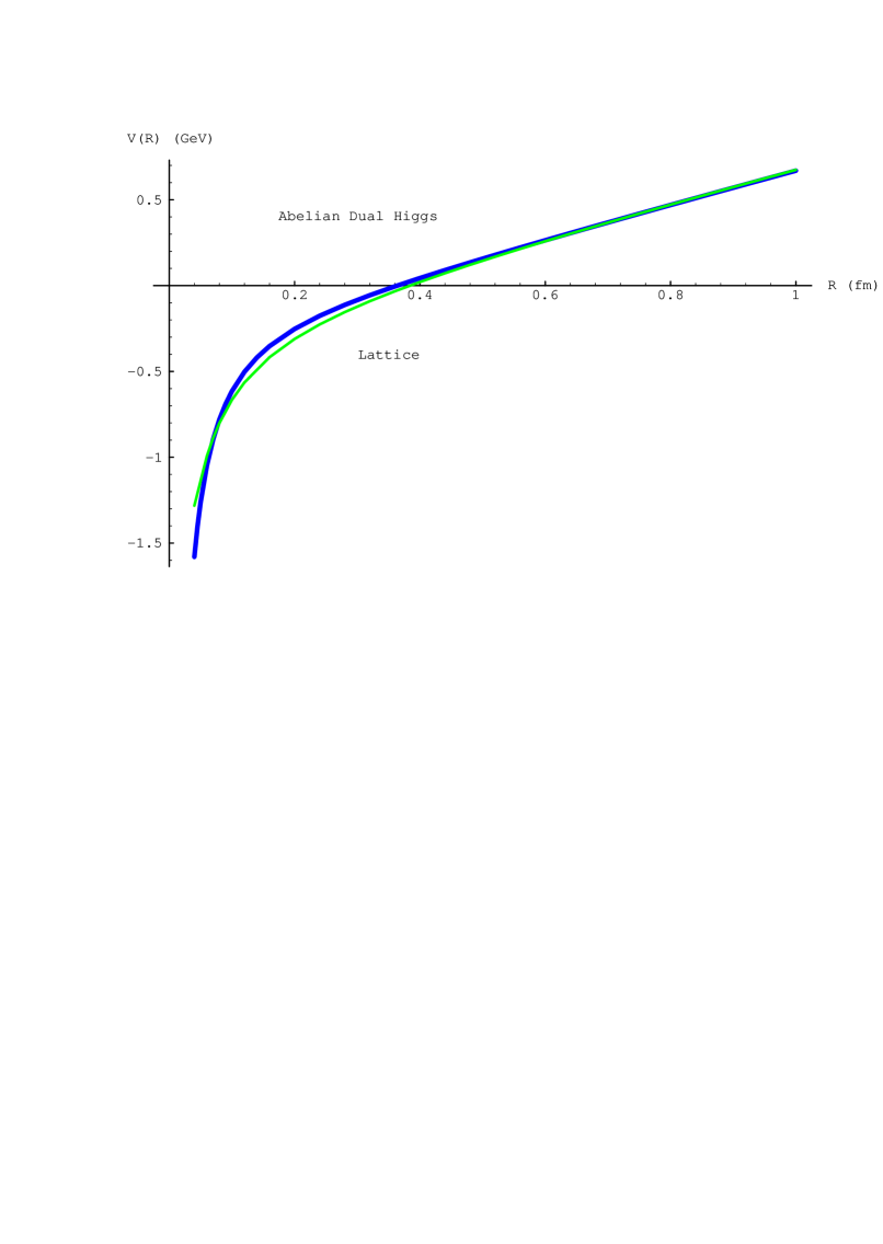
FIG. 1.: The static potential of Eq. (59) for a superconductor on the border between type I and type II with $\phi_{0}=210$ MeV, $\ell=0.22$ fm and $\displaystyle{4\over 3}{g^{2}\over 4\pi}$ = 0.32 in comparison with the lattice fit of Ref. [30].

REFERENCES

- [1] M. Shifman, A. Vainshtein and V. Zakharov, Nucl. Phys. B 147, 385, 448, 519 (1979);
- [2] M. D’Elia, A. Di Giacomo and E. Meggiolaro, Phys. Lett. B 408, 315 (1997); A. Di Giacomo, E. Meggiolaro and H. Panagopoulos, “Field strength correlations in the QCD vacuum at short distances”, IFUP-TH-12-96 (hep-lat/9603017) (1996); A. Di Giacomo and H. Panagopoulos Phys. Lett. B 285, 133 (1992);
- [3] G. S. Bali, N. Brambilla and A. Vairo, “A lattice determination of QCD field strength correlators”, HD-THEP-97-35 (hep-lat/9709079) (1997), Phys. Lett. B in press;
- [4] H. G. Dosch, Phys. Lett. B 190, 177 (1987); H. G. Dosch and Yu. A. Simonov, Phys. Lett. B 205, 339 (1988);
- [5] Yu.A. Simonov, Nucl. Phys. B 324, 67 (1989);
- [6] H. G. Dosch, Prog. Part. Nucl. Phys. 33, 121 (1994); H. G. Dosch in Proceedings of the Int. School E. Fermi, Course CXXX, Varenna 1995, (SIF1996) pag. 279; O. Nachtmann, Lectures given at the International University School of Nuclear and Particle Physics Schladming, Austria, (1996), in Schladming 1996, pag. 49 (hep-ph/9609365);
- [7] Yu. A. Simonov, Phys. Usp. 39, 313 (1996);
- [8] H. G. Dosch, E. Ferreira and A. Krämer, Phys. Rev. D 50 1992 (1994);
- [9] S. Mandelstam, Phys. Rep. 23 C, 245 (1976); G. ’t Hooft, “High Energy Physics”, Zichichi, Editrice Compositori, Bologna, 1976;
- [10] M. Rüter and H. G. Dosch, Z. Phys. C 66, 245 (1995);
- [11] M. N. Chernodub and M. I. Polikarpov, Lectures given at NATO Advanced Study Institute on Confinement, Duality and Nonperturbative Aspects of QCD, Cambridge, England, (1997) (hep-th/9710205); A. Di Giacomo (hep-th/9710080);
- [12] M. N. Chernodub, M. I. Polikarpov and A. I. Veselov, Phys. Lett. B 399, 267 (1997);
- [13] G. S. Bali, C. Schlichter and K. Schilling, “Probing the QCD vacuum with static sources in Maximal Abelian Projection” (hep-lat/9802005) (1998);
- [14] M. Baker, J. S. Ball and F. Zachariasen, Phys. Rev. D 37, 1036, 3785 (1988); Phys. Rep. 209, 73 (1991);
- [15] S. Maedan and T. Suzuki, Prog. Theor. Phys. 81, 229 (1989);
- [16] M. Baker, J. S. Ball and F. Zachariasen, Phys. Rev. D 56, 4400 (1997);
- [17] M. Baker, J. S. Ball and F. Zachariasen, Int. J. Mod. Phys. A 11, 343 (1996);
- [18] P. Pennanen, A.M. Green and C. Michael, Phys. Rev. D 56, 3903 (1997);
- [19] M. Baker, J. S. Ball, N. Brambilla, G. M. Prosperi and F. Zachariasen, Phys. Rev. D 54, 2829 (1996);
- [20] N. Brambilla and A. Vairo, Phys. Rev. D 55, 3974 (1997); M. Baker, J. S. Ball, N. Brambilla and A. Vairo, Phys. Lett. B 389, 577 (1996);
- [21] N. E. Bralic, Phys. Rev. D 22, 3090 (1980); I. Ya. Arefe’eva, Teor. Mat. Fiz. 43, 111 (1980);
- [22] Yu. A. Simonov, Yad. Fiz. 50, 213 (1989);
- [23] M. Schiestl and H. G. Dosch, Phys. Lett. B 209, 85 (1988); Yu. Simonov, Nucl. Phys. B 324, 67 (1989);
- [24] M. Eidemüller and M. Jamin, “QCD field strength correlator at the next-to-leading order”, HD-THEP-97-49 (hep-ph/9709419) (1997);
- [25] Yu. Simonov, private communications;
- [26] D. V. Antonov, “Fluctuating strings in the Universal Confining String theory and gluodynamics” (hep-th/9707245) (1997); “String representation for the ’t Hooft loop average in the Abelian Higgs model” (hep-th/9710144) (1997);
- [27] E. T. Akhmedov, M. N. Chernodub, M. I. Polikarpov and M. A.Zubkov, Phys. Rev. D 53, 2087 (1996);
- [28] M. Baker, J. S. Ball and F. Zachariasen, Phys. Rev. D 51 1968 (1995);
- [29] M. Baker, J. S. Ball and F. Zachariasen, Phys. Rev. D 44 3328 (1991);
- [30] G. S. Bali, K. Schilling and A. Wachter, Phys. Rev. D 56, 2566 (1997);
- [31] R. Akhoury, V. I. Zakharov, “On non-perturbative corrections to the potential for heavy quarks” (hep-ph/9710487) (1997);
- [32] G. S. Bali, K. Schilling and C. Schlichter, Phys.Rev. D 51, 5165 (1995).