hep-ph/9802264 SLAC–PUB–7749

February 1998 CERN–TH/98–39

UCLA/98/TEP/2

MULTI-PARTON LOOP AMPLITUDES AND NEXT-TO-LEADING ORDER JET CROSS-SECTIONS 

We review recent developments in the calculation of QCD loop amplitudes with several external legs, and their application to next-to-leading order jet production cross-sections. When a number of calculational tools are combined together — helicity, color and supersymmetry decompositions, plus unitarity and factorization properties — it becomes possible to compute multi-parton one-loop QCD amplitudes without ever evaluating analytically standard one-loop Feynman diagrams. One-loop helicity amplitudes are now available for processes with five external partons ($ggggg$, $q\bar{q}ggg$ and $q\bar{q}q^{\prime}\bar{q}^{\prime}g$), and for an intermediate vector boson $V\equiv\gamma^{*},Z,W$ plus four external partons ($Vq\bar{q}gg$ and $Vq\bar{q}q^{\prime}\bar{q}^{\prime}$). Using these amplitudes, numerical programs have been constructed for the next-to-leading order corrections to the processes $p\bar{p}\to 3$ jets (ignoring quark contributions so far) and $e^{+}e^{-}\to 4$ jets.

1 Introduction

The title of this symposium, “QCD Corrections and New Physics”, provides the motivation for this talk: Many potential signatures of new physics require a quantitative understanding of Standard Model backgrounds, which often can only be adequately provided after QCD corrections to the lowest order processes have been computed. The more partons there are in the lowest order process, the more important the QCD corrections become. On the other hand, even the first corrections, those that are next-to-leading order (NLO) in $\alpha_{s}$, have until recently only been available for processes with relatively few external partons, such as single-jet and dijet production at hadron colliders,$\!{}^{{\bf?}}$ and three-jet production in $e^{+}e^{-}$ annihilation.$\!{}^{{\bf?}}$

A major reason for this situation has been the dearth of one-loop QCD amplitudes (virtual corrections) for processes with five or more external legs. Such amplitudes are in principle straightforward to compute from Feynman rules; however, the large number of kinematic variables means that a brute-force approach can result in extremely large analytical expressions. Hence until recently one-loop amplitudes formed an ‘analytical bottleneck’ to the computation of more Standard Model processes at next-to-leading order. This talk will review techniques for systematically disentangling these amplitudes into components, primitive amplitudes, which are sufficiently simple that they can be reconstructed essentially entirely from their analytic properties, i.e. without resorting to an analytic evaluation of one-loop Feynman diagrams at all.

Some of the techniques discussed here have been used to compute the one-loop five-parton amplitudes, $ggggg$, $\!{}^{{\bf?}}$ $q\bar{q}q^{\prime}\bar{q}^{\prime}g$, $\!{}^{{\bf?}}$ and $q\bar{q}ggg$, $\!{}^{{\bf?}}$ which enter into NLO studies of the three-jet production rate and the substructure of jets at hadron colliders.$\!{}^{{\bf?},{\bf?}}$ More recently, the full set of techniques has led to the one-loop helicity amplitudes for a vector boson $V$ (which may be a virtual photon, $Z$ or $W$) plus four partons: $Vq\bar{q}q^{\prime}\bar{q}^{\prime}$ $\!{}^{{\bf?}}$ and $Vq\bar{q}gg$. $\!{}^{{\bf?},{\bf?}}$ The helicity-summed versions of the one-loop corrections to $\gamma^{*}q\bar{q}q^{\prime}\bar{q}^{\prime}$ and $\gamma^{*}q\bar{q}gg$ were calculated contemporaneously by conventional techniques,$\!{}^{{\bf?},{\bf?}}$ although the analytic formulae were too large to present. After converting to a common regularization scheme, the two sets of results agree numerically.$\!{}^{{\bf?}}$

The $Vq\bar{q}q^{\prime}\bar{q}^{\prime}$ and $Vq\bar{q}gg$ amplitudes have been used to compute the NLO corrections to $e^{+}e^{-}$ annihilation into four jets.$\!{}^{{\bf?},{\bf?},{\bf?}}$ The QCD prediction for the four-jet rate is almost doubled in going from leading order to NLO, bringing it into much better agreement with experiment, for several different jet algorithms. Besides the total four-jet rate, jet angular distributions and any other infrared-safe event-shape variable whose perturbative expansion begins at order $\alpha_{s}^{2}$ can now be computed at NLO.$\!{}^{{\bf?},{\bf?},{\bf?}}$ The latter results can be used to refine experimental measurements of the QCD color factors $C_{F}$, $C_{A}$ and $N_{f}$. The same amplitudes could also be applied to NLO processes that are related by crossing symmetry and coupling constant conversions, such as the production of a $W$ or $Z$ plus two jets at hadron colliders, or the deep inelastic production of three jets, but this has not yet been carried out.

Many aspects of the analytical techniques covered here have been previously reviewed elsewhere.$\!{}^{{\bf?},{\bf?},{\bf?},{\bf?}}$ In particular, the recent calculation of $e^{+}e^{-}\to V\to q\bar{q}gg$ required a thorough understanding of the spurious as well as physical singularities that can occur in six-point amplitudes at one loop; such details are beyond the scope of this review.

2 Primitive Amplitudes and Analytic Properties

2.1 Traditional Approaches

In the traditional approach to computing a gauge theory amplitude, one begins by drawing all Feynman diagrams. However, individual diagrams are not gauge invariant; only certain sums of diagrams are. Thus each diagram contains unphysical, gauge-variant pieces, which one would like to avoid calculating at all, since such pieces must cancel eventually. Furthermore, the standard Feynman rules for the gauge boson self-interactions induce a complicated tangle of color and Lorentz indices in each diagram. The three-gluon vertex is

$$V^{abc}_{\mu\nu\rho}(k,p,q)=f^{abc}\Bigl{(}\eta_{\nu\rho}(p-q)_{\mu}+\eta_{\rho\mu}(q-k)_{\nu}+\eta_{\mu\nu}(k-p)_{\rho}\Bigr{)}\,,$$

where $f^{abc}$ are the $SU(3)$ structure constants, $k$, $p$ and $q$ the momenta emerging from the vertex, and $\eta_{\mu\nu}$ the Minkowski metric. Each of the three terms in eq. ($(1)$) leads to a different routing of the Lorentz indices, and the composition of several $f^{abc}$s similarly leads to different routings of the color indices.

In a loop amplitude, factors of loop momenta coming from the vertices lead to further complications when one attempts to reduce the various loop integrals to a basic set of integral functions. The pentagon integral appearing in the one-loop five-gluon amplitude includes many terms with five powers of loop momenta in the numerator, arising from five vertices of the form ($(1)$). Each such term can amount to a page or more of algebra after reduction of the integral.

The complications of a diagrammatic approach are in marked contrast to the simplicity of the final results. For example, in the mid-1980s it was found that all QCD tree amplitudes with four or five external partons (and many with six or more external partons) could be written as permutation sums of simple, single-term expressions (see eq. ($(10)$)).$\!{}^{{\bf?}}$ Similarly, the one-loop four- and five-gluon amplitudes can be represented remarkably compactly (see eq. ($(12)$)).$\!{}^{{\bf?},{\bf?},{\bf?}}$

2.2 Outline of Analytic Approach

This contrast suggests that there should be a more direct and manifestly gauge-invariant way to calculate loop amplitudes than via Feynman diagrams. Here we shall advocate exploiting the two principal analytic properties of loop amplitudes, unitarity and factorization on particle poles, in a ‘perturbative bootstrap’ approach. In the old $S$-matrix bootstrap program of the 1960s,$\!{}^{{\bf?}}$ one attempted to construct $S$-matrices for the strong interactions using the constraints of analyticity. However, in the absence of a perturbative expansion, these nonlinear, coupled constraints proved too difficult to solve exactly, without imposing artificial constraints of some kind, for example on the number of states in the physical spectrum. On the other hand, in the context of perturbation theory, the constraints of $S$-matrix analyticity become recursive in the coupling constant $g$, and therefore tractable.

Figure 1: (a) Factorization of a tree amplitude on a particle pole, into the product of an $(m+1)$-point tree amplitude and an $(n-m+1)$-point tree amplitude. (b) The case $m=n-2$ (or $m=2$) corresponds to two external legs, $a$ and $b$, becoming collinear. Gray blobs represent tree amplitudes, while the hatched blob represents a splitting amplitude.

For example, an $n$-point tree amplitude is said to factorize on an intermediate particle pole when the sum of $m$ external momenta satisfies the on-shell condition for an intermediate state. The factorization condition for the massless case is $P^{2}\to 0$, where $P\equiv k_{i_{1}}+k_{i_{1}+1}+\cdots+k_{i_{2}}$. In this limit, depicted in fig. 1(a), the $n$-point amplitude becomes

 

$${{}A^{\rm tree}_{n}(1,2,\ldots,n)}$$

 

where we take all momenta to be outgoing in each amplitude, and there is an implicit sum over intermediate polarization states $\lambda$. (We have suppressed the color indices here, as is appropriate for the color-ordered primitive amplitudes defined below.) The special case $m=n-2$ (or $m=2$), shown in fig. 1(b), occurs when two of the external momenta become collinear, say $k_{a}\parallel k_{b}$:

$$A^{\rm tree}_{n}(\ldots,a,b,\ldots)\ \mathop{\longrightarrow}^{a\parallel b}\ \mathop{\rm Split}\nolimits^{\rm tree}_{-\lambda}(a^{\lambda_{a}},b^{\lambda_{b}})\,A^{\rm tree}_{n-1}(\ldots,P^{\lambda},\ldots)\,.$$

The collinear singularity behaves like the square-root of a pole, which has been absorbed into a universal splitting amplitude that replaces the second amplitude on the right-hand side of eq. ($(2)$).

The universal structure of these tree-level limits is easy to understand heuristically: The spacetime picture of the scattering process reduces to two independent scatterings connected by a single intermediate state. It can also be derived from a string-theoretic representation of the tree amplitudes.$\!{}^{{\bf?}}$ In any case, the ‘boundary values’ (factorization limits) of the $n$-point amplitude contain only lower-point amplitudes or universal functions. Thus the general $n$-point tree amplitude could be constructed recursively in $n$, simply by demanding consistency with all factorization limits, provided only that the solution to the boundary-value problem is unique. (We will discuss the uniqueness issue later.)

In fact, tree amplitudes can be constructed rather efficiently, and without any uniqueness issues, using recursive techniques based on Feynman diagrams.$\!{}^{{\bf?},{\bf?}}$ However, for loop amplitudes this is not generally the case, and so the factorization properties of loop amplitudes $\!{}^{{\bf?},{\bf?}}$ become quite useful. These properties are straightforward generalizations of the corresponding tree properties. For example, the generic form of the collinear limit of a one-loop amplitude is

 

$${A^{\rm 1\!-\!loop}_{n}(\ldots,a,b,\ldots)\ \mathop{\longrightarrow}^{a\parallel b}\ }$$

 

where $\mathop{\rm Split}\nolimits^{\rm 1\!-\!loop}$ is a new universal function.

Even more useful for loop amplitudes are the constraints imposed by unitarity. After expanding the $S$-matrix unitarity relation $S^{\dagger}S=1$ in terms of $g$, one finds that the cut or absorptive part of a one-loop $n$-point amplitude is given by the two-body phase-space integral of a product of two tree amplitudes,

 

$${A^{\rm 1\!-\!loop}_{n}(1,2,\ldots,n)\Bigr{|}_{P^{2}\ \rm cut}\!\!}$$

 

as illustrated in fig. 2. Here the cut channel has momentum squared $P^{2}$, the integration is over $D$-dimensional Lorentz-invariant phase space with with momenta $-\ell_{1}$ and $\ell_{2}$ for the intermediate states, and there is again an implicit sum over their polarizations $\lambda_{1},\lambda_{2}$. For all the one-loop multi-parton amplitudes that one might presently contemplate calculating, the tree amplitudes required to evaluate each of the cuts are readily available in a compact form.

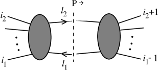
Figure 2: A cut for a one-loop amplitude, with momentum $P$ flowing across the cut. The blobs on either side of the cut represent tree amplitudes.

2.3 Decomposition into Primitive Amplitudes

Although the above factorization and unitarity constraints are powerful, they are somewhat cumbersome to implement on full multi-parton gauge theory amplitudes. It is much simpler to first identify a simpler set of gauge-invariant building blocks, called primitive amplitudes,$\!{}^{{\bf?}}$ from which the full amplitudes can be built, but which individually have simpler analytic properties. The two handles that one can use to pull apart QCD amplitudes are the helicity and color quantum numbers of the external quarks and gluons.

In massless QCD, quark helicity is conserved, and decomposing an amplitude with respect to it just amounts to inserting a helicity projector $\textstyle{1\over 2}(1\pm\gamma_{5})$ next to the external spinor. A definite gluon helicity is simplest to implement via the spinor helicity formalism,$\!{}^{{\bf?}}$ which represents gluon polarization vectors in terms of Weyl spinors $|\,k^{\pm}\rangle$,

$$\varepsilon^{+}_{\mu}(k;q)={\left\langle\smash{q}{\vphantom{1}}^{-}\right|{\gamma_{\mu}}\left|\smash{k}{\vphantom{1}}^{-}\right\rangle\over\sqrt{2}\left\langle q\,k\right\rangle}\,,\hskip 28.45274pt\varepsilon^{-}_{\mu}(k;q)={\left\langle\smash{q}{\vphantom{1}}^{+}\right|{\gamma_{\mu}}\left|\smash{k}{\vphantom{1}}^{+}\right\rangle\over\sqrt{2}\left[k\,q\right]}\,.$$

Here $k$ is the gluon momentum, $q$ is an arbitrary null ‘reference momentum’ which drops out of final gauge-invariant amplitudes, and the spinor inner-products are

$$\left\langle i\,j\right\rangle\equiv\langle k_{i}^{-}|k_{j}^{+}\rangle\,,\hskip 28.45274pt\left[i\,j\right]\equiv\langle k_{i}^{+}|k_{j}^{-}\rangle\,,\hskip 28.45274pt\left\langle i\,j\right\rangle\left[j\,i\right]=s_{ij}=(k_{i}+k_{j})^{2}\,.$$

The color structure of $SU(N_{c})$ gauge theory amplitudes can be sorted into color-ordered components — sums of contributions from Feynman graphs where the external states maintain a definite cyclic ordering with respect to each other, and where the color-ordered vertices have had the color factors removed from them.$\!{}^{{\bf?}}$ The color factors that multiply these components, in the color decomposition of the full amplitude, are ordered traces of generators $T^{a}$ for the fundamental representation of $SU(N_{c})$, ${\rm Tr}(1\ldots n)\equiv{\rm Tr}(T^{a_{1}}\ldots T^{a_{n}})$, or strings of the form $(T^{a_{3}}\cdots T^{a_{n}})_{i_{2}}^{~{}{\bar{\jmath}}_{1}}$ if external quarks are also present. For example, the color decompositions of the tree-level and one-loop five-gluon amplitudes are

$${\cal A}^{\rm tree}_{5}=g^{3}\sum_{\sigma\in S_{5}/Z_{5}}{\rm Tr}(\sigma(1)\ldots\sigma(5))A^{\rm tree}_{5}(\sigma(1),\ldots,\sigma(5))$$

and

 

$${{\cal A}_{5}^{\rm 1\!-\!loop}=}$$

 

where the permutation sums run over all inequivalent traces. $A^{\rm tree}_{5}(1,2,3,4,5)$ and $A_{5;1}(1,2,3,4,5)$ are color-ordered amplitudes, so that when their external states are chosen to be of definite helicity, e.g. $A_{5;1}(1^{\lambda_{1}},2^{\lambda_{2}},3^{\lambda_{3}},4^{\lambda_{4}},5^{\lambda_{5}})$, they qualify as primitive amplitudes. The same is not quite true of the coefficients $A_{5;3}$ of the double-trace terms in eq. ($(9)$); however, they can be expressed $\!{}^{{\bf?}}$ as sums of permutations of the $A_{5;1}$s.

The virtue of these decompositions becomes apparent when the explicit values of $A_{5}^{\rm tree}$ are recorded:

 

$${A_{5}^{\rm tree}(1^{\pm},2^{+},3^{+},4^{+},5^{+})\ }$$

 

the remaining helicity configurations are related by parity and charge conjugation.

The zeros in eq. ($(10)$) are a general consequence of supersymmetric Ward identities (SWI).$\!{}^{{\bf?}}$ At tree level, SWI can be applied directly to a non-supersymmetric theory like QCD, because no fermions can contribute to a tree-level $n$-gluon amplitude; hence the ‘missing’ fermions might as well be considered gluinos instead of quarks.$\!{}^{{\bf?}}$

The simple analytic structure of the nonzero terms is due to the color and helicity decompositions. Color-ordering implies that factorization singularities can only appear in color-adjacent channels. Thus only a subset of the kinematic variables — here, $\{s_{12},s_{23},s_{34},s_{45},s_{51}\}$ — are ‘important’ in the sense that they contain all poles (and in the loop case, all cuts) in the primitive amplitude. The denominator factors in eq. ($(10)$), $\left\langle i\,(i+1)\right\rangle=(\hbox{phase})\times\sqrt{s_{i,i+1}}$, properly capture the square-root behavior of collinear singularities, including a phase dependence as $k_{i}$ and $k_{i+1}$ are rotated around their common collinear axis; both of these factors are related to an angular-momentum mismatch of 1 unit in the collinear limit. (In other cases, $\left[i\,(i+1)\right]$ denominator factors can appear, when the mismatch has the opposite sign.)

One-loop primitive amplitudes benefit in precisely the same way as tree amplitudes from color and helicity decompositions. In addition, it is possible to decompose a one-loop amplitude according to the spins of the particles going around the loop, in a ‘supersymmetric’ way. For example, for a QCD amplitude with all external gluons, the internal gluon loop contribution $g$ (and fermion loop contribution $f$) can be rewritten as a supersymmetric contribution plus a complex scalar loop $s$,

 

$${g\ }$$

 

where $A^{N=4}$ represents the contribution of the $N=4$ super Yang-Mills multiplet, and $A^{N=1}$ an $N=1$ chiral matter supermultiplet. (Related rearrangements are possible for amplitudes with external quarks.$\!{}^{{\bf?},{\bf?}}$) The two supersymmetric contributions, $A^{N=4}$ and $A^{N=1}$, automatically obey SWI, and have other simplifications arising from loop-momentum cancellations. The scalar contribution is generally the most algebraically complicated of the three, but it is also simpler in some aspects.

We illustrate this decomposition for $A_{5;1}(1^{-},2^{-},3^{+},4^{+},5^{+})$, which is one of the two one-loop primitive amplitudes required to calculate the ‘gluonic’ NLO corrections to $p\bar{p}\to 3$ jets. Its components according to ($(11)$) are $\!{}^{{\bf?}}$

 

$${A^{N=4}}$$

 

 

$${A^{\rm scalar}}$$

 

where $c_{\Gamma}=\Gamma(1+\epsilon)\Gamma^{2}(1-\epsilon)/((4\pi)^{2-\epsilon}\Gamma(1-2\epsilon))$. Since the three components have quite different analytic structure, the rearrangement ($(11)$) is a natural one. As expected, the $A^{N=4}$ is the simplest component, followed by $A^{N=1}$. While $A^{\rm scalar}$ is the most complicated piece, it has (for example) no $s_{34}$ cut, while the full gluon loop does.

Although we do not have space to demonstrate it explicitly here, evaluation of the unitarity cuts, eq. ($(5)$), for an amplitude such as eq. ($(12)$) is quite simple. The principle reasons are:

(1) The tree amplitudes are fully ‘processed’, in terms of gauge cancellations, etc., before they are fed into the cut.

(2) SWI generally apply to the tree amplitudes, simplifying their form, even if they do not directly apply to the one-loop amplitudes.

(3) On-shell conditions for the intermediate legs, $\ell_{1}^{2}=\ell_{2}^{2}=0$, can be used repeatedly to simplify the evaluation.

The only catch to a unitarity-based approach is that loop amplitudes can have rational-function terms, containing no logarithms or dilogarithms, which are not detectable in any cut (when the cut is evaluated in four-dimensions). In eq. ($(12)$), such terms appear only in the non-supersymmetric component $A^{\rm scalar}$. (The rational-function terms in the supersymmetric components can be shown quite generally to be linked to the logarithms.$\!{}^{{\bf?}}$) Fortunately these terms can be determined using the factorization properties of loop amplitudes, such as eq. ($(4)$). One can construct an ansatz for the rational-function terms, and then proceed channel by channel to add terms to the ansatz so that it correctly reproduces the desired singular behavior in each channel, using factorization information provided by lower-point amplitudes. This procedure could fail if the factorization properties did not uniquely fix the amplitude. Although we have no formal uniqueness proof, empirically the procedure always works for six-point amplitudes. We can verify that it has worked by numerical evaluating conventional Feynman diagrams at one or more random kinematic points. (At the five-point level, there is a special term that provides a counter-example to uniqueness,$\!{}^{{\bf?}}$ although in practice its coefficient could also be fixed numerically.)

The above strategy of calculating primitive amplitudes via their unitarity cuts, with the rational-function terms fixed via factorization, has been successfully applied to the one-loop $e^{+}e^{-}\to\gamma,Z\to 4$ parton amplitudes. Most of the previously calculated one-loop four- and five-parton amplitudes reappear in this calculation as the boundary-value information for the rational-function terms, thus emphasizing the bootstrap nature of the approach.

3 Phenomenological Applications

3.1 $p\bar{p}\to 3$ jets

To date there have been two phenomenological applications of the one-loop helicity amplitudes whose calculation was outlined above. First, two groups have undertaken to compute NLO corrections to three-jet production in $p\bar{p}$ collisions.$\!{}^{{\bf?},{\bf?}}$ Production of three jets is one of the dominant processes at large transverse momentum at the Tevatron, after the one-jet inclusive and two-jet rates which have already been computed at NLO.$\!{}^{{\bf?}}$ By measuring the three-jet to two-jet ratio, once the former has been computed at NLO, one should be able to extract a relatively precise value for $\alpha_{s}(Q^{2})$, at the highest experimentally accessible values of $Q^{2}$.

Although all the matrix elements required for the full NLO $p\bar{p}\to 3$ jets calculation are available, the extreme computational demands of the numerical integrals encountered in the calculation have led both groups to perform a ‘gluonic approximation’ to the true result, in which the quark distribution functions for the proton are dropped, as well as final-state quarks. Thus only the one-loop five-gluon matrix elements $\!{}^{{\bf?}}$ and tree-level six-gluon matrix elements $\!{}^{{\bf?},{\bf?},{\bf?}}$ have to be evaluated. Although this ‘approximation’ is not expected to be particularly good quantitatively, it provides some useful qualitative lessons.

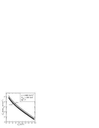
Figure 3: Dependence of the gluonic $p\bar{p}\to 3$ jet cross-section on the jet resolution parameter $d_{\rm cut}$ for the $k_{T}$ clustering algorithm.$\!{}^{{\bf?}}$ The gray and black bands result from varying the renormalization/factorization scale $\mu$ over the range $d_{\rm cut}/2<\mu<2d_{\rm cut}$ for the Born and NLO results, respectively.

Trócsányi $\!{}^{{\bf?}}$ used an iterative $k_{T}$ clustering algorithm $\!{}^{{\bf?}}$ adapted from $e^{+}e^{-}$ annihilation, with a variable jet resolution parameter $d_{\rm cut}$ which controls the overall hardness of the three-jet event. The $d_{\rm cut}$-dependence of the leading-order (Born) and NLO results are shown in fig. 3. For this jet algorithm, the Born and NLO cross-section have very similar $d_{\rm cut}$-dependence. However, the NLO result has (as expected) a much reduced dependence on the (unphysical) renormalization scale $\mu$, which bodes well for the accuracy of the full NLO three-jet rate once quark contributions are included.

Kilgore and Giele $\!{}^{{\bf?}}$ studied $p\bar{p}\to 3$ jets for the $k_{T}$ algorithm as well as for three algorithms of the cone type more commonly used at hadron colliders:

1) a ‘fixed cone’ algorithm, used by UA2, $\!{}^{{\bf?}}$

2) an ‘iterative cone’ algorithm, used by CDF and D0, $\!{}^{{\bf?}}$

3) the ‘EKS’ algorithm, used in NLO one- and two-jet inclusive calculations.$\!{}^{{\bf?}}$

Their NLO results for all but the iterative cone algorithm are shown in fig. 4. The dependence of the three-jet cross-section on the transverse energy of the leading jet, $E_{T}^{(1)}$, changes considerably between leading and next-to-leading order; it also varies with the jet algorithm.

Figure 4: The NLO gluonic $p\bar{p}\to 3$ jet cross-section as a function of the transverse energy of the leading jet, $E_{T}^{(1)}$, for three different jet algorithms and $\mu=100$ GeV, from ref. ?. See text for descriptions of the algorithms. The Born (LO) result is also shown for comparison.

There is no plot for the iterative cone algorithm — the one presently used by CDF and D0 — because Kilgore and Giele found it to be infrared unsafe for the three-jet cross-section. (See also ref. ?.) They traced this problem to final states with three hard partons, two of which are separated by slightly more than the cone size $R$. If a soft gluon is added to this configuration somewhere between these two hard partons, its only effect in the other jet algorithms will be to shift one of the three jet axes slightly. But in the iterative cone algorithm this shift will (in a subsequent step) trigger the merging of two of the three jets into one, thus altering the three-jet rate. (In fact, CDF and D0 had already introduced an additional jet separation cut when comparing their multi-jet data to leading order predictions, which effectively removed this problem, at least at NLO.) The full $p\bar{p}\to 3$ jet NLO cross-section still awaits the inclusion of quarks; however, the infrared dangers of the iterative cone algorithm already constitute a useful lesson from the gluon-only study.

3.2 $e^{+}e^{-}\to 4$ jets

A second phenomenological application has been in $e^{+}e^{-}$ annihilation. Here four-jet production, or more generally infrared-safe event-shape variables whose perturbative expansion begins at order $\alpha_{s}^{2}$, can now be studied to NLO accuracy. Such observables are sensitive to the non-Abelian self-coupling of gluons and to the production of hypothetical colored, electrically neutral particles such as light gluinos. Also, at LEP2 energies $e^{+}e^{-}\to\gamma,Z\to 4$ jets forms a significant background to $W$ pair production when both $W$s decay hadronically.

To date, two independent numerical programs for NLO corrections to generic order $\alpha_{s}^{2}$ event shapes have been constructed, MENLO_PARC $\!{}^{{\bf?}}$ and DEBRECEN,$\!{}^{{\bf?}}$ implementing the one-loop matrix elements for $e^{+}e^{-}\to\gamma,Z\to$ 4 partons, and the tree-level matrix elements for $e^{+}e^{-}\to\gamma,Z\to$ 5 partons.$\!{}^{{\bf?},{\bf?}}$ Although the two programs use different generalizations of the subtraction method $\!{}^{{\bf?},{\bf?}}$ for carrying out integrals over the singular five-parton phase-space, their results agree to within statistical errors for the Monte Carlo integration.

Figure 5: The four-jet fraction in $e^{+}e^{-}$ annihilation for the Durham jet algorithm, from ref. ?. (A small numerical error in the resummed curve has been corrected here.)

In fig. 5, QCD predictions $\!{}^{{\bf?}}$ for the four-jet fraction $R_{4}$ using the Durham jet algorithm$\!{}^{{\bf?},{\bf?}}$ are compared with data at the $Z$ pole from ALEPH $\!{}^{{\bf?}}$ and SLD,$\!{}^{{\bf?}}$ as a function of the jet resolution parameter $y_{\rm cut}$. It has long been known that the Born-level QCD prediction for the Durham (and most other $e^{+}e^{-}$ jet) algorithms, when evaluated at a renormalization scale $\mu=\sqrt{s}$, under-predicts the measured four-jet fraction by roughly a factor of two. The figure shows that addition of the NLO correction brings the prediction into much better agreement with the data, within roughly 10%.

For small values of $y_{\rm cut}$, where the four-jet fraction is large, a kinematic singularity develops in the perturbative expansion, and the true expansion parameter becomes $\alpha_{s}L^{2}$, where $L=\ln(1/y_{\rm cut})$. The Durham algorithm has the virtue of being resummable — the leading and next-to-leading logarithms at each order in $\alpha_{s}$ (terms of the form $\alpha_{s}^{n}L^{2n}$ and $\alpha_{s}^{n}L^{2n-1}$) can be calculated. In fig. 5 we also show the result of carrying out this resummation, and ‘matching’ the result to the fixed-order (NLO) calculation, which amounts to subtracting out common terms in the two expansions. This one-loop plus resummed result does improve the agreement with data still further (for $\mu=M_{Z}$) at small $y_{\rm cut}$.

Although it has been suppressed in fig. 5, the NLO prediction for $R_{4}$ still has a reasonably large uncertainty stemming from the truncation of the perturbation series after just two terms, and the large size of the second term. (This uncertainty is perhaps 20-30% if one estimates from the renormalization-scale dependence of the NLO result.) This feature limits the utility of $R_{4}$ in precision tests of QCD. On the other hand, normalized distributions for various angles between the four jets tend to have quite small, and hence reliable, NLO corrections, of order 1-3%.$\!{}^{{\bf?},{\bf?}}$

4 NNLO Predictions for Jet Physics?

Uncertainties from higher-order terms still plague NLO calculations, though not as severely as at Born level. For example, $\alpha_{s}(M_{Z}^{2})$ has been measured in $e^{+}e^{-}$ annihilation at the $Z$ pole by using a dozen or more event-shape observables $O_{i}$ whose perturbative expansion begins at order $\alpha_{s}$ (such as the three-jet fraction $R_{3}$):

 

$${O_{i}\ =\ A_{i}\left({\alpha_{s}(\mu)\over\pi}\right)}$$

 

The extracted values of $\alpha_{s}(M_{Z}^{2})$, obtained by fitting to the ${\cal O}(\alpha_{s}^{2})$ truncation of eq. ($(13)$), depend significantly on the value assumed for $\mu$ (an unphysical parameter), and on the observable used, leading to a theory uncertainty that dominates the overall error,$\!{}^{{\bf?}}$

$$\alpha_{s}(M_{Z}^{2})\ =\ 0.121\pm 0.002(\hbox{exp.})\pm 0.005(\hbox{theory}).$$

Calculation of the next-to-next-to-leading order (NNLO) ${\cal O}(\alpha_{s}^{3})$ terms in eq. ($(13)$) would clearly improve this situation.

To date, NNLO predictions in QCD are available for only a limited number of rather inclusive quantities, such as the total cross-section in $e^{+}e^{-}$ annihilation.$\!{}^{{\bf?}}$ (Because such observables have a perturbative expansion of the form $1+\alpha_{s}/\pi+\cdots$, a competitive $\alpha_{s}$ extraction requires a very high precision measurement of the observable.) NNLO results for jet physics are still a ways off; however, some of the ingredients are starting to be attacked. For the above observables $O_{i}$, three major classes of matrix elements are required:

(1) tree-level $e^{+}e^{-}\to\gamma,Z\to$ 5 partons,

(2) one-loop $e^{+}e^{-}\to\gamma,Z\to$ 4 partons,

(3) two-loop $e^{+}e^{-}\to\gamma,Z\to$ 3 partons.

As we have seen, the first two classes are now available. There will also be a considerable amount of work required in order to reliably integrate the second, and particularly the first, class of contributions over singular corners of phase space. Some steps have recently been taken along these lines.$\!{}^{{\bf?}}$

As for the two-loop matrix elements, an encouraging sign is that a complete two-loop four-gluon scattering amplitude has been computed for the first time, using generalizations of the analytic tools described above, and the result is quite compact.$\!{}^{{\bf?}}$ There are two caveats: the theory is not QCD, but $N=4$ supersymmetric $SU(N_{c})$ Yang-Mills theory; and the answer has been expressed in terms of scalar integrals, but those integrals have not yet been performed in closed form. The result for the leading-color part of the amplitude is simply

$$A_{4}^{N=4,\ {\rm 2\!-\!loop},\ {\rm L.C.}}\ =\ -N_{c}^{2}\,st\,A_{4}^{\rm tree}\left[s\,{\cal I}_{4}(s,t)+t\,{\cal I}_{4}(t,s)\right],$$

where ${\cal I}_{4}(s,t)$ is the two-loop planar double-box scalar integral,

$${\cal I}_{4}(s,t)=\!\int\!{d^{D}p\ d^{D}q\over(2\pi)^{2D}}{1\over p^{2}(p-k_{1})^{2}(p-k_{1}-k_{2})^{2}(p+q)^{2}q^{2}(q-k_{4})^{2}(q-k_{3}-k_{4})^{2}}\,.$$

Whether two-loop results can be obtained in the same way for QCD remains to be seen.

5 Conclusions

In charting the progress of particle theory from the $S$-matrix days of the 1960s, to the triumph of the Standard Model in the 1970s, to the recognition of its probable role as an effective field theory in some grander theory, Weinberg $\!{}^{{\bf?}}$ remarked: The justification of any particular effective field theory is that it is simply the most general possible theory that satisfies the axioms of analyticity, unitarity, and cluster decomposition along with the relevant symmetry principles, so in a way our use today of effective field theories is the ultimate revenge of $S$-matrix theory $\ldots$ Quantum field theory is nothing but $S$-matrix theory made practical. In some sense, the techniques reviewed here represent a further revenge of $S$-matrix theory at the computational level. Although the purely $S$-matrix-based bootstrap program of the 1960s proved intractable, the lesson here is that a perturbative bootstrap program can succeed. Once helicity, color and supersymmetry decompositions are used to break up loop amplitudes into components with simpler analytic structure, this approach becomes a particularly efficient way to compute. As a practical result, improved QCD predictions for various multi-jet processes are now emerging.

References

References

- [1] S.D. Ellis, Z. Kunszt and D.E. Soper, Phys. Rev. D40:2188 (1989); Phys. Rev. Lett. 64:2121 (1990); Phys. Rev. Lett. 69:1496 (1992); F. Aversa, M. Greco, P. Chiappetta and J.P. Guillet, Phys. Rev. Lett. 65:401 (1990); F. Aversa, L. Gonzales, M. Greco, P. Chiappetta and J.P. Guillet, Z. Phys. C49:459 (1991); W.T. Giele, E.W.N. Glover and D.A. Kosower, Phys. Rev. Lett. 73:2019 (1994); Phys. Lett. B339:181 (1994).
- [2] R.K. Ellis, D.A. Ross and A.E. Terrano, Phys. Rev. Lett. 45:1226 (1980); Nucl. Phys. B178:421 (1981); K. Fabricius, I. Schmitt, G. Kramer and G. Schierholz, Phys. Lett. B97:431 (1980); Z. Phys. C11:315 (1981).
- [3] Z. Bern, L. Dixon and D.A. Kosower, Phys. Rev. Lett. 70:2677 (1993).
- [4] Z. Kunszt, A. Signer and Z. Trócsányi, Phys. Lett. B336:529 (1994).
- [5] Z. Bern, L. Dixon and D.A. Kosower, Nucl. Phys. B437:259 (1995).
- [6] Z. Trócsányi, Phys. Rev. Lett. 77:2182 (1996) [hep-ph/9610499].
- [7] W.B. Kilgore and W.T. Giele, Phys. Rev. D55:7183 (1997) [hep-ph/9610433]; W.B. Kilgore, in Proceedings of the 1996 A.P.S. D.P.F Meeting [hep-ph/9609367]; hep-ph/9705384, to appear in proceedings of Moriond: QCD and High-Energy Hadronic Interactions, March 1997.
- [8] Z. Bern, L. Dixon, D.A. Kosower and S. Weinzierl, Nucl. Phys. B489:3 (1997) [hep-ph/9610370].
- [9] Z. Bern, L. Dixon and D.A. Kosower, Nucl. Phys. Proc. Suppl. 51C:243 (1996) [hep-ph/9606378].
- [10] Z. Bern, L. Dixon and D.A. Kosower, hep-ph/9708239, to appear in Nucl. Phys. B.
- [11] E.W.N. Glover and D.J. Miller, Phys. Lett. B396:257 (1997) [hep-ph/9609474].
- [12] J.M. Campbell, E.W.N. Glover and D.J. Miller, Phys.Lett.B409:503 (1997) [hep-ph/9706297].
- [13] J.M. Campbell and E.W.N. Glover, private communication.
- [14] A. Signer and L. Dixon, Phys. Rev. Lett. 78:811 (1997) [hep-ph/9609460].
- [15] A. Signer and L. Dixon, Phys. Rev. D56:4031 (1997) [hep-ph/9706285].
- [16] Z. Nagy and Z. Trócsányi, Phys. Rev. Lett. 79:3604 (1997) [hep-ph/9707309]; hep-ph/9708344, to appear in proceedings of QCD 97, July 1997.
- [17] A. Signer, hep-ph/9705218, to appear in proceedings of Moriond: QCD and High-Energy Hadronic Interactions, March 1997.
- [18] Z. Nagy and Z. Trócsányi, hep-ph/9712385.
- [19] Z. Bern, L. Dixon and D.A. Kosower, Ann. Rev. Nucl. Part. Sci. 46:109 (1996) [hep-ph/9602280].
- [20] L. Dixon, in QCD & Beyond: Proceedings of TASI ’95, ed. D.E. Soper (World Scientific, 1996) [hep-ph/9601359].
- [21] Z. Bern, L. Dixon and D.A. Kosower, Nucl. Phys. Proc. Suppl. 51C:243 (1996) [hep-ph/9606378]; L. Dixon, hep-ph/9507214, in Proceedings of SUSY95, eds I. Antoniadis and H. Videau (Editions Frontieres, 1996); Z. Bern, L. Dixon, D.C. Dunbar and D.A. Kosower, hep-ph/9706447, to appear in proceedings of DIS 97.
- [22] M. Mangano and S.J. Parke, Phys. Rep. 200:301 (1991).
- [23] Z. Bern and D.A. Kosower, Nucl. Phys. 379:451 (1992).
- [24] Z. Kunszt, A. Signer and Z. Trócsányi, Nucl. Phys. B411:397 (1994).
- [25] S. Mandelstam, Phys. Rev. 112:1344 (1958); G.F. Chew and S.C. Frautschi, Phys. Rev. 123:1486 (1961); G.F. Chew and A. Pignotti, Phys. Rev. 176:2112 (1968).
- [26] F.A. Berends and W.T. Giele, Nucl. Phys. B306:759 (1988).
- [27] D.A. Kosower, Nucl. Phys. B335:23 (1990); G. Mahlon and T.-M. Yan, Phys. Rev. D47:1776 (1993), hep-ph/9210213; G. Mahlon, Phys. Rev. D47:1812 (1993), hep-ph/9210214; G. Mahlon, T.-M. Yan and C. Dunn, Phys. Rev. D48:1337 (1993) [hep-ph/9210212].
- [28] Z. Bern, L. Dixon, D.C. Dunbar and D.A. Kosower, Nucl. Phys. B425:217 (1994), hep-ph/9403226.
- [29] Z. Bern and G. Chalmers, Nucl. Phys. B447:465 (1995), hep-ph/9503236; G. Chalmers, hep-ph/9405393, in Proceedings of the XXII ITEP International Winter School of Physics (Gordon and Breach, 1995).
- [30] P. De Causmaecker, R. Gastmans, W. Troost and T.T. Wu, Phys. Lett. 105B:215 (1981), Nucl. Phys. B206:53 (1982); R. Kleiss and W.J. Stirling, Nucl. Phys. B262:235 (1985); R. Gastmans and T.T. Wu, The Ubiquitous Photon: Helicity Method for QED and QCD (Clarendon Press, 1990); Z. Xu, D.-H. Zhang and L. Chang, Nucl. Phys. B291:392 (1987).
- [31] M.T. Grisaru, H.N. Pendleton and P. van Nieuwenhuizen, Phys. Rev. D15:996 (1977); M.T. Grisaru and H.N. Pendleton, Nucl. Phys. B124:81 (1977).
- [32] S.J. Parke and T. Taylor, Phys. Lett. 157B:81 (1985); Z. Kunszt, Nucl. Phys. B271:333 (1986).
- [33] Z. Bern, L. Dixon, D.C. Dunbar and D.A. Kosower, Nucl. Phys. B435:39 (1995) [hep-ph/9409265].
- [34] S. Parke and T. Taylor, Nucl. Phys. B269:410 (1986); Z. Kunszt, Nucl. Phys. B271:333 (1986); J. Gunion and J. Kalinowski, Phys. Rev. D34:2119 (1986); F.A. Berends and W.T. Giele, Nucl. Phys. B294:700 (1987); M. Mangano, S. Parke and Z. Xu, Nucl. Phys. B298:653 (1988).
- [35] S. Catani, Yu.L. Dokshitser and B.R. Webber, Phys. Lett. B285:291 (1992); S. Catani, Yu.L. Dokshitser, M.H. Seymour and B.R. Webber, Nucl. Phys. B406:187 (1993); see also S.D. Ellis and D. Soper, Phys. Rev. D48:3160 (1993) [hep-ph/9305266].
- [36] UA2 Collab., Phys. Lett. B257:232 (1991).
- [37] CDF Collab., Phys. Rev. D45:1448 (1992); D0 Collab., Phys. Rev. D53:6000 (1996) [hep-ex/9509005].
- [38] S.D. Ellis, Z. Kunszt and D.E. Soper, Phys. Rev. Lett. 62:726 (1989).
- [39] M.H. Seymour, hep-ph/9707338.
- [40] A. Signer, Comput. Phys. Commun. 106:125 (1997).
- [41] F.A. Berends, W.T. Giele and H. Kuijf, Nucl. Phys. B321:39 (1989).
- [42] K. Hagiwara and D. Zeppenfeld, Nucl. Phys. B313:560 (1989); N.K. Falck, D. Graudenz and G. Kramer, Nucl. Phys. B328:317 (1989).
- [43] R.K. Ellis, D.A. Ross and A.E. Terrano, Phys. Rev. Lett. 45:1226 (1980); Nucl. Phys. B178:421 (1981).
- [44] Z. Kunszt and D.E. Soper, Phys. Rev. D46:192 (1992); S. Frixione, Z. Kunszt and A. Signer, Nucl. Phys. B467:399 (1996) [hep-ph/9512328]; S. Catani and M.H. Seymour, Phys. Lett. B378:287 (1996) [hep-ph/9602277], Nucl. Phys. B485:291 (1997) [hep-ph/9605323].
- [45] N. Brown and W.J. Stirling, Z. Phys. C53:629 (1992).
- [46] S. Catani, Yu.L. Dokshitser, M. Olsson, G. Turnock and B.R. Webber, Phys. Lett. B269:432 (1991).
- [47] ALEPH Collab., R. Barate et al., preprint CERN-PPE-96-186, to appear in Phys. Rep.
- [48] SLD Collab., K. Abe et al., Phys. Rev. Lett. 71:2528 (1993); P. Burrows (SLD Collab.), private communication.
- [49] For a review, see P. Burrows, Acta Phys. Polon. B28:701 (1997) [hep-ex/9612007].
- [50] S.G. Gorishny, A.L. Kataev and S.A. Larin, Phys. Lett. B259:144 (1991); L.R. Surguladze and M.A. Samuel, Phys. Rev. Lett. 66:560 (1991); erratum ibid. 66:2416 (1991).
- [51] A. Gehrmann-De Ridder and E.W.N. Glover, hep-ph/9707224; J.M. Campbell and E.W.N. Glover, hep-ph/9710255.
- [52] Z. Bern, J.S. Rozowsky and B. Yan, Phys. Lett. B401:273 (1997) [hep-ph/9702424]; hep-ph/9706392, to appear in proceedings of DIS 97.
- [53] S. Weinberg, in The Rise of the Standard Model, eds. L. Hoddeson, L. Brown, M. Riordan and M. Dresden (Cambridge, 1997).