NUC-MINN-97/13-T Multiple Scattering Expansion of the Self-Energy at Finite Temperature

Abstract

An often used rule that the thermal correction to the self-energy is the thermal phase-space times the forward scattering amplitude from target particles is shown to be the leading term in an exact multiple scattering expansion. Starting from imaginary-time finite-temperature field theory, a rigorous expansion for the retarded self-energy is derived. The relationship to the thermodynamic potential is briefly discussed.

I Introduction

At a temperature much lower than the particle mass, it is physically reasonable to expect that the leading order thermal correction to the physical self-energy be given by the forward scattering amplitude integrated over the thermal phase-space of the lighter particle. For instance, in the literature, the thermal self-energy of a particle is often written as [1, 2, 3]

$$\Sigma_{T}(p)=-\int{d^{3}k\over(2\pi)^{3}2E_{\hbox{light}}}\,n(E_{\hbox{light}})\,{\cal T}(k+p\to k+p)\;,$$ (1)

where $E_{\hbox{light}}=\sqrt{{\bf k}^{2}+m_{\hbox{light}}^{2}}$ is the energy of the lighter particle with mass $m_{\hbox{light}}$, $n(E_{\hbox{light}})$ is a Bose or Fermi distribution function, and ${\cal T}(k+p\to k+p)$ is the forward scattering amplitude related to the usual $f$ by

$${\cal T}(k+p\to k+p)=8\pi\sqrt{s}\,f(k,p)\;.$$ (2)

The minus sign on the right hand side of Eq. (1) stems from the fact that the scattering amplitude is defined to be $-i$ times an $N$-point correlation function whereas the self-energy is defined to be $i$ times a 2-point correlation function.

A merit of this method is that one can simply take the scattering amplitudes from experiment. In reactions involving strong couplings, this may be the only reliable way of calculating the thermal correction to the real part of the self-energy [4]. As the density and temperature become higher, Eq. (1) needs higher order corrections. In this paper, we start with the imaginary-time formulation of relativistic finite temperature field theory and obtain an exact expression for the thermal self-energy.

There are a variety of finite temperature field theory methods used in literature. The real-time method was first investigated by Schwinger and Keldysh and later in a slightly different and modern form by many people [5, 6, 7, 8, 9]. The imaginary-time method was introduced by Matsubara [10] and through analytic continuation can be related to the real-time method [11]. Of course any equilibrium Green function can be calculated using any of the methods, given the analytic relations between them.

There are, however, situations where one particular method is more economical. For instance, if one would like to study time-ordered real-time correlation functions, the real-time method is very much the natural choice. If one would like to study a response function (a retarded function), the most economical way would be to compute the imaginary-time correlation function with Matsubara frequencies and then analytically continue the result.

In this paper we are interested in the retarded correlation functions. We would like to use the imaginary-time method. However, since the imaginary time is a fictitious parameter introduced to deal with the temperature, it is not easy to gain physical insight by just looking at the end result of the imaginary time calculation. A way to remedy this difficulty was developed by one of the present authors [12] based on earlier works [13, 14, 15]. There, a diagrammatic method to calculate the spectral density of two-point functions in a scalar theory was presented, starting from the imaginary-time formulation of finite temperature field theory. Subsequently it was used to calculate the leading order hydrodynamic coefficients in a scalar theory [16]. In this paper the above work is extended to the calculation of $N$-point retarded functions.

The analysis in this paper is based on the fact that applying the analytic continuation

$$i\nu\to k^{0}+i\epsilon$$ (3)

to each of the independent external Matsubara frequencies produces the (Fourier transformed) retarded correlation function [9, 17]. When the chemical potentials all vanish, this operation produces the physical retarded function. However, with non-zero chemical potentials one must be more careful.

In the imaginary-time formalism, finite density is dealt with by using an effective Hamiltonian

$$\hat{K}\equiv\hat{H}-\sum_{a}\mu_{a}\hat{Q}_{a}\;,$$ (4)

where $\mu_{a}$ is the chemical potential associated with each conserved charge $\hat{Q}_{a}$. Hence, the retarded function produced by using Eq. (3) corresponds to the retarded correlation function of $\hat{\varphi}_{K}(t)\equiv e^{i\hat{K}t}\hat{\varphi}e^{-i\hat{K}t}$. But the physical retarded function is a correlation function of $\hat{\varphi}_{H}(t)\equiv e^{i\hat{H}t}\hat{\varphi}e^{-i\hat{H}t}$, not $\hat{\varphi}_{K}(t)$. Fortunately, there is a simple relation between the two. In most cases the fields of interest are charge eigenstates. Then

$$\hat{\varphi}_{K}(t)=e^{i\mu_{\varphi}t}\hat{\varphi}_{H}(t)\;,$$ (5)

where

$$\mu_{\varphi}=\sum_{a}\mu_{a}q_{a}$$ (6)

is the total chemical potential associated with the field $\varphi$ carrying conserved charges $q_{a}$. In momentum space, the two retarded functions are related by [18]

$$G_{\varphi_{H}}^{\hbox{Ret}}(\{k\})=G_{\varphi_{K}}^{\hbox{Ret}}(\{k-\mu_{\varphi}\})\;,$$ (7)

where we used a shorthand notation, $k-\mu_{\varphi}\equiv(k^{0}-\mu_{\varphi},{\bf k})$. As is shown in Sec. II B, this shift also has the effect of separating the purely dynamic part of the theory and the purely statistical part.

This paper is organized as follows. In Sec. II a brief derivation is given for the diagrammatic rules to compute an arbitrary retarded function. Section III presents a derivation of the self-energy formula using the results from Sec. II. As an example, the self-energy of an electron at the one-loop level is worked out in Sec. IV. Finally, we conclude in Sec. V. Appendices A and B list some relevant facts about the finite temperature propagators used in this paper. Appendix C deals with derivative couplings. Appendix D amplifies the discussion of the thermodynamic potential in Sec. III.

II $N$-point Retarded Correlation Functions

In this section, as a prelude to the self-energy calculation, diagrammatic rules to calculate an arbitrary $N$-point retarded function are derived starting from imaginary-time finite temperature field theory. The derivation here closely follows Ref. [12]. Details omitted for the sake of brevity and readability can be found in that reference and references therein. The rules derived here coincide with the rules obtained by Evans [9] who used the real-time method and the analytic relations between $N$-point functions. For simplicity, only theories involving no derivative couplings are considered here. However, the argument given here can be straightforwardly generalized to theories with derivative couplings, such as chiral perturbation theory, as indicated in Appendix C.

A Euclidean Correlation Functions

It is known that performing Matsubara frequency sums in an Euclidean Feynman diagram produces terms corresponding to old-fashioned time-ordered perturbation theory [14]. The aim here is therefore to provide conventions and definitions along with a sketch of a proof, but not the details. A detailed derivation for a relativistic case can be found in Ref. [12] and a non-relativistic version can be found in Ref. [13].

The standard Feynman rules use the momentum space Feynman propagator. For our purposes, it is more convenient to use mixed propagators which are functions of time and spatial momentum. As shown in Appendix A, the mixed propagator for both bosons and fermions can be represented by

$$G_{\zeta}(\tau,{\bf k})=\int{d\omega\over 2\pi}\,N_{\zeta}(\omega)\,\left(e^{-\omega\tau}\,\rho^{+}_{\zeta}(k)\,\theta(\tau)\,+e^{\omega\tau}\,\rho^{-}_{\zeta}(k)\,\theta(-\tau)\,\right)\;.$$ (8)

Here $\omega\equiv k^{0}$, and the spectral densities are labeled $\rho^{\pm}_{\zeta}(k)$ or $\rho_{\zeta}^{\pm}(\omega,{\bf k})$, as convenient. The label $\zeta$ distinguishes boson or fermion, $\{\hbox{B, F}\}$. The statistical factor $N_{\zeta}(\omega)$ is

$$N_{\zeta}(\omega)=1+(-1)^{\zeta}n_{\zeta}(\omega)\;,$$ (9)

where $(-1)^{\rm B}\equiv 1$ and $(-1)^{\rm F}\equiv-1$ and

$$n_{\zeta}(\omega)={1\over e^{\omega\beta}-(-1)^{\zeta}}\;.$$ (10)

Explicit forms for the spectral densities are not of interest in this section. What is important for us is that they satisfy

$$\rho^{+}_{\zeta}(\omega,{\bf k})=-\rho^{-}_{\zeta}(-\omega,{\bf k})$$ (11)

due to the periodicity or antiperiodicity of $G_{\zeta}(\tau,{\bf k})$ in $\tau$. A few relevant facts about the spectral densities are given in Appendices A and B.

The Feynman rules in this mixed space of imaginary-time and momentum are almost identical to the standard momentum space Feynman rules. The differences are: An imaginary-time $\tau_{j}$ labels each vertex including the external ones. Each line connecting two vertices labeled by the times $\tau_{a}$ and $\tau_{b}$ represents a propagator $G_{\zeta}(\tau_{a}{-}\tau_{b},|{\bf k}|)$ if the momentum flows from $\tau_{b}$ to $\tau_{a}$. If the momentum flows from $\tau_{a}$ to $\tau_{b}$, the line represents $G_{\zeta}(\tau_{b}{-}\tau_{a},|{\bf k}|)$. The direction of the momentum should follow the direction of charge flow. Instead of the sum over all loop frequencies, there are integrations over all $\tau_{j}$’s from $0$ to $\beta$. At each vertex where an external field operator extracts external frequency $i\nu_{j}$ an additional factor of $\exp\left(i\nu_{j}\tau_{j}\right)$ is present. Hence, the contribution of a connected Feynman diagram $\Gamma$ with a total of $V{+}1$ vertices and $N{+}1$ external operator insertions has the following schematic form:

$$C_{N+1}^{(\Gamma)}(\{{\bf q}_{l},i\nu_{l}\})$$ (12)

$$= \int_{0}^{\beta}\prod_{i=0}^{V}d\tau_{i}\exp\left(i\sum_{l=0}^{N}\nu_{l}\tau_{l}\right)\,\int\prod_{L\in\Gamma}{d^{3}k_{L}\over(2\pi)^{3}}\,A_{V+1}^{N+1}$$ (14)

$${}\times\prod_{\alpha\in\Gamma}\int{d\omega_{\alpha}\over 2\pi}\,N_{\zeta_{\alpha}}(\omega_{\alpha})\,\left(e^{-\omega_{\alpha}(\tau_{a}-\tau_{b})}\,\rho^{+}_{\zeta_{\alpha}}(k_{\alpha})\,\theta(\tau_{a}-\tau_{b})\,+e^{\omega_{\alpha}(\tau_{a}-\tau_{b})}\,\rho^{-}_{\zeta_{\alpha}}(k_{\alpha})\,\theta(\tau_{b}-\tau_{a})\,\right)\;.$$

Here the independent spatial loop momenta are denoted by ${\bf k}_{L}$, and the quantity $A_{V+1}^{N+1}$ includes all the factors from interaction vertices such as coupling constants, $\gamma$ matrices, and symmetry factors. We suppress Lorentz indices, if there are any, since they are not relevant for the moment. A given line in the Feynman diagram running between vertices acting at times $\tau_{a}$ and $\tau_{b}$ is denoted by $\alpha$.

We know that as the temperature goes to zero the result of the time integrations must be that of old-fashioned time-ordered perturbation theory. That is,

$$\lim_{\beta\to\infty}C_{N+1}^{(\Gamma)}(\{{\bf q}_{l},i\nu_{l}\})=\sum_{{\Gamma_{\sigma}}\subset\Gamma}\;\lim_{\beta\to\infty}C_{N+1}^{(\Gamma_{\sigma})}(\{{\bf q}_{l},i\nu_{l}\})\;,$$ (16)

where $\sigma$ represents a given permutation of the vertices and $\Gamma_{\sigma}$ represents a time-ordered diagram for that permutation given by

$$\lim_{\beta\to\infty}C_{N+1}^{(\Gamma_{\sigma})}(\{{\bf q}_{l},i\nu_{l}\})$$ (17)

$$= \int\prod_{L\in\Gamma}{d^{3}k_{L}\over(2\pi)^{3}}\,\prod_{\alpha\in\Gamma}\left(\int{d\omega_{\alpha}\over 2\pi}\,\theta(\omega_{\alpha})\,\rho_{\zeta_{\alpha}}^{s_{\sigma}}(k_{\alpha})\right)\,A_{V+1}^{N+1}\prod_{{\hbox{{\rm intervals}}\atop\hbox{$\scriptstyle{V\geq j\geq 1}$}}}\Bigl{(}\Lambda_{j}^{\sigma}-i\nu_{j}^{\sigma}\Bigr{)}^{-1}\;.$$ (18)

Here we omit the overall frequency-conserving Kronecker-$\delta$. The sign $s_{\sigma}=\{+,-\}$ depends on both the time ordering and the direction of the charge flow. If the charge flows in the same direction as the time a $+$ sign is assigned, otherwise $s_{\sigma}=-$. If there are no conserved charges the distinction is without significance. The prefactor $A_{V+1}^{N+1}$ is the same as before. The time ordering also determines the frequency denominator $(\Lambda_{j}^{\sigma}-i\nu_{j}^{\sigma})$. Given a time ordering $\sigma$, $\Lambda_{j}^{\sigma}$ is given by the sum of frequencies of all lines crossing the $j$-th interval $I_{j}^{\sigma}$

$$\Lambda_{j}^{\sigma}=\sum_{\alpha\in I_{j}^{\sigma}}\omega_{\alpha}\;.$$ (19)

Similarly, $\nu_{j}^{\sigma}$ is the net external frequency flowing out of the diagram above the interval $I_{j}^{\sigma}$

$$\nu_{j}^{\sigma}=\sum_{V\geq l\geq j}\nu_{l}\;.$$ (20)

In this limit the external frequencies $\nu_{l}$ are continuous.

Comparing Eq. (18) and Eq. (14) one sees that one should keep all factors of $N_{\zeta}(\omega_{\alpha})$ since

$$\lim_{\beta\to\infty}N_{\zeta}(\omega_{\alpha})=\theta(\omega_{\alpha})\;.$$ (21)

Then for Eq. (18) to be true, there cannot be any additional factors of $\exp\left\{\pm\beta\sum_{i}\omega_{i}\right\}$ in the finite temperature result since they will make the result diverge due to the fact that frequencies can be both positive and negative. The structure of integrand in Eq. (14) also dictates that vanishing contributions such as $\exp\left\{-\beta|\sum_{i}\omega_{i}|\right\}$ or $1/\beta^{n}$ cannot occur. Then the only feasible non-zero temperature result is Eq. (18) with $\theta(\omega_{\alpha})$ replaced by $N_{\zeta_{\alpha}}(\omega_{\alpha})$. That is,

$${C}_{N{+}1}^{(\Gamma)}(\{{\bf q}_{l},i\nu_{l}\})=\sum_{{\Gamma_{\sigma}}\subset\Gamma}\;C_{N+1}^{(\Gamma_{\sigma})}(\{{\bf q}_{l},i\nu_{l}\})\;,$$ (22)

where

$$C_{N+1}^{(\Gamma_{\sigma})}(\{{\bf q}_{l},i\nu_{l}\})$$ (23)

$$= \int\prod_{L\in\Gamma}{d^{3}k_{L}\over(2\pi)^{3}}\,\prod_{\alpha\in\Gamma}\left(\int{d\omega_{\alpha}\over 2\pi}\,N_{\zeta_{\alpha}}(\omega_{\alpha})\,\rho_{\zeta_{\alpha}}^{s_{\sigma}}(k_{\alpha})\right)\,A_{V+1}^{N+1}\prod_{{\hbox{{\rm intervals}}\atop\hbox{$\scriptstyle{V\geq j\geq 1}$}}}\Bigl{(}\Lambda_{j}^{\sigma}-i\nu_{j}^{\sigma}\Bigr{)}^{-1}\;,$$ (24)

again omitting the overall frequency-conserving Kronecker-$\delta$.

B Retarded Correlation Functions

The $(N{+}1)$-point retarded function is defined by [19]

$$R(x;\{x_{i}\})\equiv$$ (26)

$$\sum_{\sigma}\theta(t{-}t_{\sigma_{1}})\,\prod_{j=1}^{N-1}\theta(t_{\sigma_{j}}{-}t_{\sigma_{j+1}})\,\Big{\langle}[...[[\hat{\varphi}(x),\hat{\varphi}_{\sigma_{1}}(x_{\sigma_{1}})],\hat{\varphi}_{\sigma_{2}}(x_{\sigma_{2}})],...,\hat{\varphi}_{\sigma_{N}}(x_{\sigma_{N}})]\Big{\rangle}\,,$$

where $t=x^{0}$ is the fixed largest time, $i$ runs from 1 to $N$, and $\sum_{\sigma}$ indicates the sum over all possible permutation of $\{t_{1},t_{2},\ldots,t_{N}\}$. The operator $\hat{\varphi}$ can be any field in the theory. When two fermionic quantities are involved, the commutator becomes an anti-commutator. The angular bracket represents the thermal average. From here on, we always denote by $v$ the vertex at fixed time $t$.

Several authors [9, 17] have shown that the following analytic continuation of the $(N{+}1)$-point imaginary-time correlation function leads to the retarded function:

$$i\nu_{l} \to q_{l}^{0}+i\epsilon\ \ \hbox{for}\ \ l\neq v$$ (27)

$$i\nu_{v} \to q_{v}^{0}+iN\epsilon\;,$$ (28)

where at vertices other than the fixed time vertex $v$ the frequencies are injected, and at $v$ the frequency is extracted so that the frequency is conserved including the small imaginary part:

$$q_{v}^{0}+iN\epsilon=\sum_{l\neq v}(q_{l}^{0}+i\epsilon)\;.$$ (29)

The contribution of a Feynman diagram $\Gamma$ to the retarded function ${R}_{N{+}1}^{(\Gamma_{v})}(\{q_{l}\})$ (subscript $v$ signifies that $v$ is the fixed vertex) is then:

$${R}_{N{+}1}^{(\Gamma_{v})}(\{q_{l}\}) = \displaystyle\sum_{{\Gamma_{\sigma}}\subset\Gamma}\;\int\prod_{L\in\Gamma}{d^{3}k_{L}\over(2\pi)^{3}}\,\prod_{\alpha\in\Gamma}\left(\int{d\omega_{\alpha}\over 2\pi}\,N_{\zeta_{\alpha}}(\omega_{\alpha})\,\rho_{\zeta_{\alpha}}^{s_{\sigma}}(k_{\alpha})\right)A_{V+1}^{N+1}$$ (31)

$$\qquad{}\times\prod_{{\hbox{{\rm intervals}}\atop\hbox{$\scriptstyle{V\geq j\geq v+1}$}}}\Bigl{(}\Lambda_{j}^{\sigma}-q^{\sigma}_{j}+i\epsilon\Bigr{)}^{-1}\prod_{{\hbox{{\rm intervals}}\atop\hbox{$\scriptstyle{v\geq j^{\prime}\geq 1}$}}}\Bigl{(}\Lambda_{j^{\prime}}^{\sigma}-q^{\sigma}_{j^{\prime}}-i\epsilon\Bigr{)}^{-1}\;.$$

The $\Lambda_{j}^{\sigma}$ were defined in Eq. (19) and the quantities $q^{\sigma}_{j}$ refer to the net external frequency flowing out of the diagram above the given interval

$$q^{\sigma}_{j}=\sum_{V\geq v_{l}\geq j}q^{0}_{l}\;.$$ (32)

Here we chronologically label the vertices by $\{t_{0},\cdots,t_{V}\}$ and the interval between $t_{j}$ and $t_{j-1}$ is the $j$-th interval. Also, a product without a factor is defined to be 1. Note the change in the sign of the $\epsilon$ term when crossing the $v$-th interval. The sign depends on whether the interval is above or below the vertex $v$ which extracts $iN\epsilon$. Intervals where no external frequencies flow in or out have no $i\epsilon$ to start with, but it is not hard to make the internal frequencies slightly off the real axis to make a consistent assignment of the imaginary parts [12].

We would like to express Eq. (31) in terms of uncut and cut propagators in analogous fashion to the Cutkosky approach at zero temperature. To that end, notice that if all the $+i\epsilon$’s in the frequency denominators were $-i\epsilon$ and all the $N_{\zeta_{\alpha}}(\omega_{\alpha})$ were $\theta(\omega_{\alpha})$, then the expression would be exactly that of old-fashioned real-time perturbation theory. When the time orderings are summed, this expression just reproduces the Feynman diagram expression. Hence when all the small imaginary parts are $-i\epsilon$, all we need to do to sum the time-ordered terms is to change the zero temperature propagator

$$G^{0}_{\zeta}(k)=\int{d\omega\over 2\pi i}\,\theta(\omega)\,\left({\rho_{\zeta}^{+}(\omega,|{\bf k}|)\over\omega-k^{0}-i\epsilon}+{\rho_{\zeta}^{-}(\omega,|{\bf k}|)\over\omega+k^{0}-i\epsilon}\right)\,$$ (33)

to the finite temperature one

$$G_{\zeta}(k)\equiv\int{d\omega\over 2\pi i}\,N_{\zeta}(\omega)\,\left({\rho_{\zeta}^{+}(\omega,|{\bf k}|)\over\omega-k^{0}-i\epsilon}+{\rho_{\zeta}^{-}(\omega,|{\bf k}|)\over\omega+k^{0}-i\epsilon}\right)\,\;,$$ (34)

see Appendix B. Then

$$D_{N{+}1}^{(\Gamma)}(\{q_{l}\}) \equiv \sum_{\Gamma_{\sigma}\subset\Gamma}\int\prod_{L\in\Gamma}{d^{3}k_{L}\over(2\pi)^{3}}\,\prod_{\alpha\in\Gamma}\left(\int{d\omega_{\alpha}\over 2\pi}\,N_{\zeta_{\alpha}}(\omega_{\alpha})\,\rho_{\zeta_{\alpha}}^{s_{\sigma}}(\omega_{\alpha},|{\bf k}_{\alpha}|)\right)A_{V+1}^{N+1}$$ (36)

$$\qquad\qquad{}\times\prod_{{\hbox{{\rm intervals}}\atop\hbox{$\scriptstyle{V\geq j\geq 1}$}}}\Bigl{(}\Lambda_{j}^{\sigma}-q^{\sigma}_{j}-i\epsilon\Bigr{)}^{-1}$$

$$= -i(i)^{V+1}\int\prod_{L\in\Gamma}{d^{4}k_{L}\over(2\pi)^{4}}\,A_{V+1}^{N+1}\prod_{\alpha\in\Gamma}G_{\zeta_{\alpha}}(k_{\alpha})\;.$$ (37)

The factor $-i(i)^{V+1}$ comes from having $V$ integrals with $-i\epsilon$. The phase $i^{V+1}$ can be absorbed into $A_{V+1}^{N+1}$ by adding a factor of $i$ to the coupling constant at each vertex as in the usual diagram rules, e.g. see Peskin and Schroeder [20] whose conventions we follow.

We would like to apply this argument to each of the $\pm i\epsilon$ parts of the product in ${R}_{N{+}1}^{(\Gamma_{v})}(\{q_{l}\})$. In order to do so, the two parts must be separated from each other so that the lines common to both parts can be regarded as external ones. This is achieved by using the identity

$$0=\prod_{j=v+1}^{V}\Bigl{(}U_{j}{-}i\epsilon\Bigr{)}^{-1}-\prod_{j=v+1}^{V}\Bigl{(}U_{j}{+}i\epsilon\Bigr{)}^{-1}-i\sum_{l=v+1}^{V}2\pi\delta(U_{l})\prod_{k=l+1}^{V}\Bigl{(}U_{k}{+}i\epsilon\Bigr{)}^{-1}\prod_{j=v+1}^{l-1}\Bigl{(}U_{j}{-}i\epsilon\Bigr{)}^{-1}\;.$$ (38)

Here all $U_{j}$’s are real, a sum without a summand is 0 and a product without a factor is 1. This identity follows directly from $2\pi i\delta(x)=(x-i\epsilon)^{-1}-(x+i\epsilon)^{-1}$. We refer to the lines corresponding to the interval in $\delta(U_{l})$ as the cut lines.

Using the above identity and performing the relevant resummation of time ordered terms on both sides of the cut, we obtain

$${R}_{N{+}1}^{(\Gamma_{v})}(\{q_{l}\})={D}_{N{+}1}^{(\Gamma)}(\{q_{l}\})+\sum_{{\Gamma\hbox to0.0pt{\hss${\scriptstyle-}$}}_{v}\subset\Gamma}{R}_{N{+}1}^{({\Gamma\hbox to0.0pt{\hss${\scriptstyle-}$}}_{v})}(\{q_{l}\})\;,$$ (39)

where

$$R^{({\Gamma\hbox to0.0pt{\hss${\scriptstyle-}$}}_{v})}_{N+1}(\{q_{l}\}) = -i(-i)^{V_{+}}(i)^{V_{-}}\int\prod_{L\in\Gamma}{d^{4}k_{L}\over(2\pi)^{4}}\,A_{V+1}^{N+1}\prod_{{\hbox{{\rm cut lines}}\atop\hbox{{\it c}}}}\left(N_{\zeta_{c}}(k^{0}_{c})\,\rho_{\zeta_{c}}^{s_{c}}(k_{c})\right)$$ (41)

$$\qquad\qquad\qquad\qquad{}\times\prod_{\alpha\in\Gamma_{+}}G_{\zeta_{\alpha}}(k_{\alpha})^{*}\,\prod_{\alpha^{\prime}\in\Gamma_{-}}G_{\zeta_{\alpha^{\prime}}}(k_{\alpha^{\prime}})\;,$$

and the sum is over the cut diagrams ${\Gamma\hbox to0.0pt{\hss$-$}}_{v}$. The uncut propagator $G_{\zeta}$ corresponds to the lines in the side $\Gamma_{-}$ which contains $v$, and $G_{\zeta}^{*}$ corresponds to the lines in the other side $\Gamma_{+}$. For the cut lines the direction of time flow is from $\Gamma_{-}$ to $\Gamma_{+}$. Here $V_{\pm}$ denotes number of vertices in $\Gamma_{\pm}$. Again, the factors $(-i)^{V_{+}}(i)^{V_{-}}$ can be absorbed into $A_{V+1}^{N+1}$ by including a factor of $i$ in the contribution of each vertex in $\Gamma_{-}$ and a factor of $-i$ in the contribution of each vertex in $\Gamma_{+}$.

So far, nothing has been dependent on the presence of chemical potentials. When chemical potentials are present, Eq. (39) corresponds to the retarded function of fields $\hat{\varphi}_{K}(t)=e^{i\hat{K}t}\hat{\varphi}e^{-i\hat{K}t}$ with $\hat{K}=\hat{H}-\sum_{a}\mu_{a}\hat{Q}_{a}$. As explained in Sec. I, there is a simple relation between $\hat{\varphi}_{K}$ and $\hat{\varphi}_{H}$, $\hat{\varphi}_{K}(t)=e^{i\mu_{\varphi}t}\hat{\varphi}_{H}(t)$. Hence, to convert a retarded function of the $\hat{\varphi}_{K}$ to the corresponding retarded function of the $\hat{\varphi}_{H}$, all one has to do is to shift each external frequency from $q$ to $q-\mu_{\varphi}$ if it corresponds to the particle of the species and to $q+\mu_{\varphi}$ if it corresponds to the anti-particle. These shifts have important simplifying consequences. Due to charge conservation, not only energy-momentum, but also chemical potential has to be conserved at each vertex. Hence, shifting the external frequency $q^{0}\to q^{0}-\mu_{\varphi}$ is equivalent to shifting all internal frequencies $l^{0}\to l^{0}-\mu_{\alpha}$ according to the species $\alpha$.

The significance of these internal frequency shifts is that they remove the chemical potential dependence from the spectral densities. For instance, when the chemical potential is non-zero, the spectral density of the bosonic propagator appearing in Eq. (31) is (see Appendix A)

$$\rho^{+}_{\rm B}(k^{0})={\rm sign}(k^{0}+\mu)\,2\pi\,\delta\left((k^{0}+\mu)^{2}-E_{k}^{2}\right)\;,$$ (42)

where $E_{k}=\sqrt{{\bf k}^{2}+m^{2}}$. By shifting $k^{0}\to k^{0}-\mu$, $\rho^{+}_{\rm B}(k^{0}-\mu)$ becomes independent of $\mu$, while the same change will make the statistical factor become $n_{\rm B}(\omega-\mu)$.

For small chemical potentials such that $m_{\zeta}>|\mu_{\zeta}|$, even more simplification is possible because in that case, $\theta(E\pm\mu)=\theta(E)$ and $\theta(-E\pm\mu)=\theta(-E)$. Then

$$N_{\zeta}(k^{0}-\mu)=\theta(k^{0})+(-1)^{\zeta}{\rm sign}(k^{0})n_{\zeta}(|k^{0}-\mu|)\;,$$ (43)

when $k^{0}=\pm E_{k}$. Consequently, the chemical potential only appears in the statistical factors. In this way we achieve the separation of the statistical part and the purely dynamic part of the particle propagation. (For a slightly different approach, see [21]).

We can now state diagrammatic rules for calculating an arbitrary $N$-point retarded function with small chemical potentials $(|\mu_{\zeta}|<m_{\zeta})$, see Appendix B for further details. For convenience, we denote the thermal phase space factor for scalar bosons by

$$\Gamma_{\rm B}(k)=n_{B}(|k^{0}-\mu|)\,2\pi\,\delta(k^{2}-m^{2})$$ (44)

and for spin-$\frac{1}{2}$ fermions

$$\Gamma_{\rm F}(k)=-n_{\rm F}(|k^{0}-\mu|)\,(k^{\mu}\gamma_{\mu}+m)\,2\pi\,\delta(k^{2}-m^{2})\;.$$ (45)

Define the cut propagators for scalar particles

$$\Delta_{\rm B}^{\pm}(k)=\theta(\pm k^{0})\,2\pi\,\delta(k^{2}-m^{2})+\Gamma_{\rm B}(k)\;,$$ (46)

and for fermions,

$$\Delta_{\rm F}^{\pm}(k)=\theta(\pm k^{0})\,2\pi\,(k^{\mu}\gamma_{\mu}+m)\,\delta(k^{2}-m^{2})+\Gamma_{\rm F}(k)\;.$$ (47)

For scalar particles, the uncut propagators are given by

$$G_{\rm B}(k)={i\over k^{2}-m^{2}+i\epsilon}+\Gamma_{\rm B}(k)\ \ \hbox{and}\ \ G^{*}_{\rm B}(k)={-i\over k^{2}-m^{2}-i\epsilon}+\Gamma_{\rm B}(k)$$ (48)

and for spin-$\frac{1}{2}$ fermions, they are given by

$$G_{\rm F}(k)={i(k^{\mu}\gamma_{\mu}+m)\over k^{2}-m^{2}+i\epsilon}+\Gamma_{\rm F}(k)\ \ \hbox{and}\ \ G^{*}_{\rm F}(k)={-i(k^{\mu}\gamma_{\mu}+m)\over k^{2}-m^{2}-i\epsilon}+\Gamma_{\rm F}(k)\;.$$ (49)

For gauge bosons, set $m=0$ in each of the scalar particle propagator, and multiply by $(-g_{\mu\nu})$ (Feynman gauge). Note that all of the cut and uncut propagators can be written as a zero-temperature, zero-density part plus a common thermal phase space factor. Not surprisingly, the zero temperature parts of the propagators all coincide with the zero-temperature Cutkosky rule propagators [22].

We call the region where the fixed vertex $v$ sits the unshaded region and the other half the shaded region. The rules to calculate the retarded functions of $\hat{\varphi}_{H}$ are:

1. Draw all topologically distinct cut diagrams including totally uncut ones, keeping the largest time always on the unshaded side. Disconnected pieces produced by the cutting are allowed.

2. Assign momenta to the lines according to the flow of the conserved charges, if there are any.

3. Use the usual Feynman rules for the unshaded side assigning $G_{\zeta}(k)$ to the uncut lines.

4. Use the complex conjugate Feynman rules for the shaded side assigning $G_{\zeta}^{*}(k)$ to the uncut lines. The $\gamma$ matrices are not to be complex conjugated.

5. If the momentum $k$ of a cut line crosses from the unshaded region to the shaded region, assign $\Delta_{\zeta}^{+}(k)$.

6. If the momentum $k$ of a cut line crosses from the shaded region to the unshaded region, assign $\Delta_{\zeta}^{-}(k)$.

7. Divide by the symmetry factor if applicable. There is an overall factor of $-i$.

Equation (39) and the above diagrammatic rules are the main results of this section. As shown in Appendix C, this same set of rules also apply when there are derivative couplings.

As an example of applying the rules, consider a scalar theory with a $-g\phi^{3}$ interaction in the Lagrangian. The diagram shown in Fig. 1 yields the expression

$$C^{\hbox{fig.{\ref{fig:example}}}}(k) = (-i)(-ig)^{4}(ig)^{2}\int{d^{4}l\over(2\pi)^{4}}\,{d^{4}p\over(2\pi)^{4}}\,{d^{4}q\over(2\pi)^{4}}\,\Delta_{\rm B}^{+}(l)\,\Delta_{\rm B}^{+}(p)\,\Delta_{\rm B}^{-}(q)\,\Delta_{\rm B}^{-}(l{+}p{-}q)\,$$ (51)

$$\qquad\qquad\qquad\qquad{}\times G_{\rm B}(l{+}p{-}q{-}k)\,G_{\rm B}(l{-}k)\,G_{\rm B}(p{-}q)\,G^{*}_{\rm B}(l{+}p)\;.$$

Note that at $T=0$, the contribution of this diagram is zero because the cut part then represents a process where four physical particles annihilate each other into the vacuum. At non-zero temperature, this diagram gives a non-zero contribution because it can also represent scattering between physical particles in the thermal medium.

FIG. 1.: A typical finite temperature cut diagram in a scalar $g\phi^{3}$ theory. Each cut line contributes $\Delta_{\rm B}^{+}$ or $\Delta_{\rm B}^{-}$ according to its orientation. In the unshaded (shaded) region, an uncut propagator contributes $G_{\rm B}$ ($G_{\rm B}^{*}$), and an interaction vertex contributes a factor of $-ig$ $(ig)$.

III Multiple Scattering Expansion of the Self-Energy

In this section, we present the multiple scattering expansion for the thermal contribution to the self-energy. The retarded self-energy is, of course, a retarded 2-point function. From the previous section (see also Appendix B) we know that as long as $m_{a}>|\mu_{a}|$, all propagators satisfy

$$D_{\zeta}(k)=D_{\zeta}^{0}(k)+\Gamma_{\zeta}(k)$$ (52)

where $\Gamma_{\zeta}(k)$ is the thermal phase space factor common to all four cut and uncut propagators, and $D_{\zeta}^{0}(k)$ is the zero temperature, zero density propagator.

Using Eq. (52) we can now expand the expression (39) for the self-energy in the number of $\Gamma_{\zeta}$’s. The coefficients in this expansion involve only the zero temperature propagators. Hence, the coefficient function is either a zero-temperature Feynman diagram or a zero-temperature Cutkosky diagram. External momenta for this coefficient function are provided by the self-energy momentum, $k$, and the thermal particle momenta from the $\Gamma_{\zeta}$’s.

We would like to relate the coefficients of the expansion to the physical zero-temperature scattering amplitudes. In order to do so, we need to ensure that in the expansion we consider:

1. Symmetry factors are all correctly accounted for.

2. Disconnected parts cancel.

3. Self-energy insertions do not cause divergences.

4. Additional polarization factors needed for the external thermal particles are all correctly provided.

5. When fermions are involved, the overall sign for an individual Feynman diagram is correctly produced.

We present the result of the expansion first and deal with the above points later in Subsecs. III A–III C.

We emphasize that the formal expansion in the number of $\Gamma_{\zeta}$’s can be always made. To be useful, however, the series must be truncated. When the temperature and the density are low so that $T\ll|m_{a}\pm\mu_{a}|$ for all particle species $a$, one may order the expansion with respect to the relative strengths of $e^{-(m_{a}-\mu_{a})/T}$ and $e^{-(m_{a}+\mu_{a})/T}$. The first few terms of such a virial expansion will be a good approximation as long as the densities and the temperature stay low. As the densities and the temperature grow so that the minimum of $|m_{a}\pm\mu_{a}|$ is no longer small compared to the temperature, we lose control of the approximation because, potentially, an infinite number of terms in the expansion become important.

The diagrams that provide the thermal contributions to the retarded self-energy, $\Sigma^{\hbox{Ret}}_{T}$, can be separated into three groups, as depicted in Fig. 2. Group (a) contains no cut, group (b) contains cuts that do not separate the two external vertices and group (c) contains cuts that do separate the two external vertices.

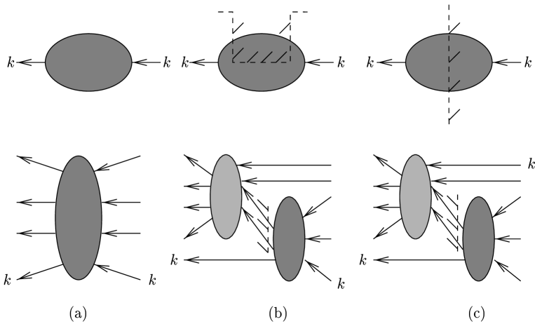
FIG. 2.: Diagrams that contribute to the self-energy. The upper row is illustrated in more detail in the lower row.

Consider first the diagrams depicted in Fig. 2(a). The diagrams in this group are solely made of the uncut propagator $G_{\zeta}(l)=G_{\zeta}^{0}(l)+\Gamma_{\zeta}(l)$, where $G_{\zeta}^{0}(l)$ is the zero temperature Feynman propagator and $\Gamma_{\zeta}(l)$ is the thermal phase space factor. When the expansion in the number of $\Gamma_{\zeta}$ is made, the coefficients are obviously the zero temperature Feynman diagrams whose external momenta are supplied by the self-energy momentum and the thermal particle momenta from the $\Gamma_{\zeta}$’s. That is, the coefficients correspond to matrix elements of the scattering operator ${\cal T}$, with the $S$-matrix given by ${\cal S}=1+i{\cal T}$. Hence, the expansion of the first group of the diagrams can be written as

$$\Sigma^{\hbox{(a)}}_{T}(k) = -\sum_{n\geq 2,\sigma}{1\over S_{\{l_{i}^{\sigma}\}}}\int\prod_{i=1}^{n-1}d\Gamma_{i}^{\sigma}\,\langle k,\{l_{i}^{\sigma}\}|{\cal T}|k,\{l_{i}^{\sigma}\}\rangle_{\hbox{conn}}$$ (54)

$${}+\left(\hbox{disconnected diagrams}\right)\;,$$

where

$$d\Gamma_{i}^{\sigma}\equiv\frac{d^{3}l_{i}}{(2\pi)^{3}2E_{i}}n_{\zeta_{i}}(E_{i}-\sigma\mu_{i})\;,$$ (55)

with $E_{i}=\sqrt{{\bf l}_{i}^{2}+m_{i}^{2}}$ and $\sigma=+1$ for a particle and $-1$ for an antiparticle. In Eq. (54) the symmetry factor is denoted by $S_{\{l_{i}^{\sigma}\}}$; this will be discussed in the following subsection.

Next consider the diagrams of Fig. 2(b) shown schematically in the upper row and in more detail in the lower row. To express these diagrams in terms of the scattering operator, we define an operator ${\cal T}_{k}$ such that

$$\langle k,\{l_{i}^{\sigma}\}|{\cal T}_{k}|\{p_{i}\}\rangle \equiv \langle k,\{l_{i}^{\sigma}\}|{\cal T}|\{p_{i}\}\rangle-(\hbox{disconnected parts involving $\delta(k-p_{i})$})$$ (56)

and

$$\langle\{p_{i}\}|{\cal T}_{k}|k,\{l_{i}^{\sigma}\}\rangle \equiv \langle\{p_{i}\}|{\cal T}|k,\{l_{i}^{\sigma}\}\rangle-(\hbox{disconnected parts involving $\delta(k-p_{i})$})\;.$$ (57)

We also define

$${\Delta}_{k}\equiv{\cal T}-{\cal T}_{k}\;.$$ (58)

The coefficients originating from expanding a cut diagram in this second group must also contain a cut with the same restriction that the two external vertices should always be in the unshaded region. Hence, the coefficient functions are the zero temperature Cutkosky diagrams with the same restriction. We know that the zero temperature Cutkosky diagrams represent matrix element of ${\cal T}^{\dagger}{\cal T}$. Hence, the expansion of this group of diagrams must be

$$\Sigma^{\hbox{(b)}}_{T}(k) = i\sum_{n\geq 2,\sigma}{1\over S_{\{l_{i}^{\sigma}\}}}\int\prod_{i=1}^{n-1}d\Gamma_{i}^{\sigma}\,\sum_{\{p_{j}\}}\langle\{l_{i}^{\sigma}\}|{\cal T}^{\dagger}|\{p_{j}\}\rangle\langle k,\{p_{j}\}|{\cal T}|k,\{l_{i}^{\sigma}\}\rangle|_{\hbox{conn}}$$ (60)

$${}+\left(\hbox{disconnected diagrams}\right)$$

$$= i\sum_{n\geq 2,\sigma}{1\over S_{\{l_{i}^{\sigma}\}}}\int\prod_{i=1}^{n-1}d\Gamma_{i}^{\sigma}\,\langle k,\{l_{i}^{\sigma}\}|{\Delta}_{k}^{\dagger}{\cal T}_{k}|k,\{l_{i}^{\sigma}\}\rangle|_{\hbox{conn}}$$ (62)

$${}+\left(\hbox{disconnected diagrams}\right)\;.$$

The third group of diagrams contain a cut that separates the external vertices as shown in Fig. 2(c). Noting that the external frequency $k$ flows out of the unshaded region and the cut-line frequencies flow into the shaded region, we can write

$$\Sigma^{\hbox{(c)}}_{T}(k) = i\sum_{n\geq 2,\sigma}{1\over S_{\{l_{i}^{\sigma}\}}}\int\prod_{i=1}^{n-1}d\Gamma_{i}^{\sigma}\,\sum_{\{p_{j}\}}\langle\{l_{i}^{\sigma}\}|{\cal T}^{\dagger}|k,\{p_{j}\}\rangle\langle k,\{p_{j}\}|{\cal T}|\{l_{i}^{\sigma}\}\rangle|_{\hbox{conn}}$$ (64)

$${}+\left(\hbox{disconnected diagrams}\right)$$

$$= i\sum_{n\geq 2,\sigma}{1\over S_{\{l_{i}^{\sigma}\}}}\int\prod_{i=1}^{n-1}d\Gamma_{i}^{\sigma}\,\langle k,\{l_{i}^{\sigma}\}|\Delta_{k}^{\dagger}\Delta_{k}|k,\{l_{i}^{\sigma}\}\rangle|_{\hbox{conn}}$$ (66)

$${}+\left(\hbox{disconnected diagrams}\right)\;.$$

Ignoring the disconnected diagrams which will later be shown to cancel, the three contributions yield

$$\Sigma^{\hbox{Ret}}_{T}(k) = \Sigma^{\hbox{(a)}}_{T}(k)+\Sigma^{\hbox{(b)}}_{T}(k)+\Sigma^{\hbox{(c)}}_{T}(k)$$ (67)

$$= -\sum_{n\geq 2,\sigma}{1\over S_{\{l_{i}^{\sigma}\}}}\int\prod_{i=1}^{n-1}d\Gamma_{i}^{\sigma}\,\langle k,\{l_{i}^{\sigma}\}|\left({\cal T}-i{\Delta}_{k}^{\dagger}{\cal T}\right)|k,\{l_{i}^{\sigma}\}\rangle_{\hbox{conn}}$$ (68)

$$= -\sum_{n\geq 2,\sigma}{1\over S_{\{l_{i}^{\sigma}\}}}\int\prod_{i=1}^{n-1}d\Gamma_{i}^{\sigma}\,\langle k,\{l_{i}^{\sigma}\}|{\cal T}_{k}^{\dagger}{\cal S}|k,\{l_{i}^{\sigma}\}\rangle_{\hbox{conn}}\;,$$ (69)

where we used $\langle k,\{l_{i}^{\sigma}\}|{\cal T}_{k}|k,\{l_{i}^{\sigma}\}\rangle_{\hbox{conn}}=\langle k,\{l_{i}^{\sigma}\}|{\cal T}|k,\{l_{i}^{\sigma}\}\rangle_{\hbox{conn}}$, Eq. (58) and the identity ${\cal T}={\cal T}^{\dagger}{\cal S}={\cal T}^{\dagger}(1+i{\cal T})$.

We can now show that Eq. (1) is the lowest order approximation of the expansion (69). Without self-energy insertions, the matrix element $\langle k,l|{\Delta}_{k}^{\dagger}{\cal T}|k,l\rangle_{\hbox{conn}}$ vanishes provided that the momentum $l$ represents a stable particle which cannot decay at $T=0$. The lightest particle in a theory is certainly stable. Hence, Eq. (1) holds at the lowest order in the density expansion.

To check the consistency of Eq. (69), consider the imaginary part,

$${\rm Im}\,\Sigma^{\hbox{Ret}}_{T}(k) = -{1\over 2}\sum_{n\geq 2,\sigma}{1\over S_{\{l_{i}^{\sigma}\}}}\int\prod_{i=1}^{n-1}d\Gamma_{i}^{\sigma}\,\langle k,\{l_{i}^{\sigma}\}|\left({\cal T}^{\dagger}_{k}{\cal T}_{k}-{\Delta}_{k}^{\dagger}\Delta_{k}\right)|k,\{l_{i}^{\sigma}\}\rangle_{\hbox{conn}}\;.$$ (70)

Here we used the unitarity condition ${\rm Im}\,{\cal T}={1\over 2}{\cal T}^{\dagger}{\cal T}$ to get Eq. (70) from the second line of Eq. (69). The cut diagrams leading to expression (70) must contain cuts that separate the two external vertices. Also the diagrams corresponding to ${\cal T}_{k}^{\dagger}{\cal T}_{k}$ must have the external momentum $k$ entering the unshaded region, while those corresponding to $\Delta_{k}^{\dagger}\Delta_{k}$ must have the external momentum $k$ exiting the unshaded region. In Ref. [12] it is shown that these cut diagrams are exactly the diagrams that gives the spectral density of the 2-point correlation function. The retarded self-energy is the negative of a 2-point retarded correlation function with a real spectral density (see Appendix A). This implies that

$${\rm Im}\,\Sigma^{\hbox{Ret}}(k)=-{\textstyle{1\over 2}}\,\chi^{\vphantom{x}}_{\Sigma}(k)\;,$$ (71)

where $\chi^{\vphantom{x}}_{\Sigma}(\omega)$ is the spectral density for the self-energy. This is consistent with Eq. (70).

Eq. (69) can quickly be used to make contact with the thermal ($T>0$) part of the thermodynamic grand potential; for a more rigorous discussion see Appendix D. We need to close off the diagrams of Fig. 2 by including a propagator for the external line $k$. The zero temperature part will give a contribution that can be included in the scattering matrices, while the finite temperature part gives an additional $d\Gamma$ integration and the symmetry factor must be appropriately adjusted. We note that in Eq. (69) ${\cal T}_{k}^{\dagger}{\cal S}={\cal T}_{k}^{\dagger}\sum_{m=0}^{\infty}\left(i{\cal T}^{\dagger}\right)^{m}$. When the propagator for $k$ is included, ${\cal T}_{k}^{\dagger}$ is no longer distinguished from ${\cal T}^{\dagger}$, but we must include a factor of $(m+1)^{-1}$ in the sum in order to avoid multiple counting. Thus we have $-i\sum_{m=0}^{\infty}\left(i{\cal T}^{\dagger}\right)^{m+1}/(m+1)=i\ln\left(1-i{\cal T}^{\dagger}\right)$. Thus the thermal part of the grand potential can be written

$${\Omega_{T}\over V} = -i\sum_{n\geq 2,\sigma}{1\over S_{\{l_{i}^{\sigma}\}}}\int\prod_{i=1}^{n}d\Gamma_{i}^{\sigma}\,\langle\{l_{i}^{\sigma}\}|\ln(1-i{\cal T}^{\dagger})|\{l_{i}^{\sigma}\}\rangle_{\hbox{conn}}$$ (72)

$$= i\sum_{n\geq 2,\sigma}{1\over S_{\{l_{i}^{\sigma}\}}}\int\prod_{i=1}^{n}d\Gamma_{i}^{\sigma}\,\langle\{l_{i}^{\sigma}\}|\ln(1+i{\cal T})|\{l_{i}^{\sigma}\}\rangle_{\hbox{conn}}\;,$$ (73)

where $V$ denotes the volume of the system and in the last step we have used the reality of $\Omega$. We have also assumed that the physical mass of the particles is used in the propagators so that diagrams with a single thermal weighting are superfluous. Equation (73) agrees with Norton’s version [23] of the expression originally given by Dashen, Ma and Bernstein [21].

A Symmetry factors

There are two issues involving the symmetry factor, $S_{\{l_{i}^{\sigma}\}}$, arising in the equations above. One involves the symmetry factor due to the self-interaction. For instance, the two loop diagram in a $\lambda\phi^{4}$ theory shown in Fig. 3 has the symmetry factor of $S_{\hbox{2-loop}}=3!$ since the three internal lines are equivalent to each other. Our density expansion inevitably reduces the symmetry of this diagram. One needs to show that the expansion in the number of $\Gamma_{\zeta}$ automatically generates the symmetry factor associated with the reduced symmetry in such cases. The second issue involves identical particles. When there are $m$ identical particles in the final state, the $m$-body phase-space includes a factor of $1/m!$. Our expansion must also automatically account for this factor.

To see that the symmetry factors are correctly generated, we label each line in a diagram by $l_{\alpha}$ and each vertex by $\tau_{a}$ and regard them as distinguishable. The symmetry group $G$ of a given Feynman diagram then represents the permutations of the internal lines and the vertices that does not change the shape of the diagram [24]. The order $q_{G}$ of this group is the symmetry factor for the diagram. For example, the symmetry group of the two-loop diagram in Fig. 3 is the full permutation group of the three identical lines. Hence, $S_{\hbox{2-loop}}=q_{G}=3!$.

FIG. 3.: A 2-loop diagram in scalar $\lambda\phi^{4}$ theory.

Consider a cut diagram for the self-energy. The density expansion essentially amounts to the sum of all possible ways of mixing the zero-temperature propagators and the thermal phase space factors without totally disconnecting the diagram. In such “divided diagrams” the lines and the vertices in the original diagram are apportioned into the thermal part (which solely consists of $\Gamma_{\zeta}$’s) and the zero-temperature part.

In general this partitioning will reduce the symmetry group of the original group $G$ to a subgroup $S$. The reduced symmetry group $S$ is then a product group consisting of the symmetry groups $S_{\rm z}$ and $S_{\rm t}$ of the two parts. Here the subscript ‘z’ represents the zero-temperature part, and the subscript ‘t’ represents the thermal part. In other words the symmetry group is now,

$$S=S_{\rm z}\otimes S_{\rm t}\;.$$ (74)

The order of this product group is of course $q_{S}=q_{\rm z}\times q_{\rm t}$, where $q_{\rm z}$ and $q_{\rm t}$ are the order of the subgroups $S_{\rm z}$ and $S_{\rm t}$, respectively. We must show that the density expansion automatically generates the symmetry factor $q_{S}=q_{\rm z}\times q_{\rm t}$ associated with the reduced diagram.

It is well known in group theory that the order of a subgroup is a factor of the order of the full group [25]. That is, $q_{G}/q_{S}=r$ is an integer. We would like to show that there are exactly $r$ different partitions of the original lines and vertices that result in the same divided diagram. Then we show that the correct symmetry factor is produced for each individual diagram in our expansion.

To see how it works out, suppose the symmetry group $G$ of the original diagram is of order $q_{G}$, and when divided into zero-temperature and thermal parts, the symmetry group reduces to a subgroup $S$ of order $q_{S}$. Consider the right coset,

$$G/S=\{Sg_{1},Sg_{2},\cdots,Sg_{q_{G}}\}\;,$$ (75)

where each $g_{i}\in G$ is a permutation acting on the internal vertices and the lines that does not change the shape of the original diagram. Since the identity must be an element of $G$ and the $Sg_{i}$’s are either identical or disjoint, we can rewrite

$$G/S=\{S_{1},S_{2},\cdots,S_{r}\}\;,$$ (76)

where $S_{1}=S$, $S_{i}$’s are all disjoint, each $S_{i}$ has $q_{S}$ elements, and $r=q_{G}/q_{S}$ [25].

Operating with $s_{i}\in S_{1}$ on the diagram does not change the partition of the lines and vertices since $S_{1}=S$ is the symmetry group of the divided diagram. However, the other $S_{i}$’s must contain at least one element that corresponds to a different partition. Then there exist $h_{i}$’s such that $h_{i}\in G$ and

$$S_{i}=Sh_{i}=\{h_{i},s_{2}h_{i},s_{3}h_{i},\cdots,s_{q_{S}}h_{i}\}\;.$$ (77)

Here, $s_{i}\in S$, $s_{1}=I$ and $h_{1}=I$. Since $S_{i}$ and $S_{j}$ are disjoint for $i\neq j$, we have $h_{i}\neq h_{j}$. The number of $h_{i}$’s is then equal to $r=q_{G}/q_{S}$. Also each element of $S_{i}$ is related to $h_{i}$ by an element of $S$. This implies that all elements in $S_{i}$ correspond to the same partition of the lines and vertices. Hence the total number of inequivalent partitions of the internal lines and vertices is exactly the same as the number of $h_{i}$’s. Consequently, when our density expansion is made, the coefficient of a divided diagram is $r/q_{G}=1/(q_{\rm z}\times q_{\rm t})$. Thus the symmetry factor associated with the symmetry of the divided diagram is always correctly produced by the density expansion.

As a simple example, consider the 2-loop diagram shown in Fig. 3. If one of the lines is opened out so that it carries a thermal phase space factor as shown in the first of Fig. 4, the symmetry group is reduced to the permutation of the two remaining lines so that the overall factor becomes $1/2!$. Originally, $q_{G}=3!$, and now $q_{S}=2!$. The ratio $q_{G}/q_{S}=3$ of course corresponds to the three choices we can make when selecting a line to replace.

If two lines from the diagram in Fig. 3 are opened out and carry thermal weightings, we produce the second diagram in Fig. 4. The symmetry group of the reduced diagram is the trivial identity. Hence, the symmetry factor associated with the reduced diagram is 1. However, since there are only ${}_{3}C_{2}=3$ choices of picking a pair of lines, the overall factor for the second diagram in Fig. 4 is only $3/3!=1/2!$. This is as it should be because the thermal lines have a reflection symmetry.

FIG. 4.: Density expansion of the 2-loop diagram in Fig. 3. The dot at the end of a line denotes that the line corresponds to a thermal particle.

To make the connection between opened-up self-energy diagrams, such as those in Fig. 4, and the ${\cal T}$-matrices label the latter with 2 $k$’s, $m$ initial momenta $p_{i}$ and $m$ final momenta $q_{i}$. Eventually, we identify $p_{i}=q_{i}$ and integrate over the thermal phase-space of all $p_{i}$’s to make the contribution to the self-energy. Suppose that all $p_{i}$ and $q_{i}$ belong to the same species. Then the matrix elements

$${\cal T}(k,p_{1},\ldots,p_{m};k,q_{1},\ldots,q_{m})$$

and

$${\cal T}(k,p_{\sigma_{1}},\ldots,p_{\sigma_{m}};k,q_{\sigma_{1}},\ldots,q_{\sigma_{m}})\;,$$

where $\sigma$ is one of the $m!$ permutation of $\{1,\ldots,m\}$, correspond to the same self-energy diagram when the $p_{i}$’s are integrated over the thermal phase space.

Even though there are $m!$ such permutations, the number of distinct ${\cal T}(k,\{p\};k,\{q\})$ need not equal $m!$. For some permutations, the above two expressions may not only give the same contribution to the self-energy, but actually be the same even before the integration. If we reconnect the $p_{i}$ vertices with the $q_{i}$ vertices, the resulting diagram is a self-energy diagram. Hence the number of permutations giving rise to the same ${\cal T}$ must be equal to the order $q_{\rm t}$ of the symmetry group $S_{\rm t}$ of the reconnected part of the diagram. Hence, the coefficient of this reconnected diagram is given by $m!/(q_{\rm t}\times q_{\rm z})$ where $q_{\rm z}$ is the symmetry factor associated with the ${\cal T}$.

Comparing this with $1/(q_{\rm t}\times q_{\rm z})$ which we had for the opened-up self-energy diagram, we see that a diagram generated from the self-energy is smaller by a factor of $m!$ than an actual scattering amplitude diagram. The generalization to the many species case is immediate. Thus if each particle species $i$ has $m_{i}$ external thermally-weighted lines, the overall factor for the opened-up self-energy diagram is $1/S_{\{l_{i}^{\sigma}\}}~{}=~{}1/\prod_{i}m_{i}!$.

B Disconnected Parts

Suppose that, when the internal lines are opened out and given thermal weightings $\Gamma_{\zeta}$, we get a disconnected piece containing at least one internal vertex. As long as this disconnected piece does not contain the largest time vertex, all cuts for this diagram, including the case with no cuts at all, are possible with the rest of the original diagram being kept common. For the isolated subdiagram, this situation corresponds to having all the frequency denominators in Eq. (38) and summing over all time orderings. Consequently, the net contribution of such a disconnected part vanishes. In the real-time method this cancellation is referred to as the vanishing of the sum of all circlings [5].

For an elementary example, consider the sum of all cut and uncut propagators depicted in Fig. 5.

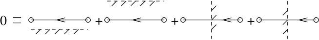
FIG. 5.: Cancelling propagators.

The sum is

$$(-i)^{2}G_{\zeta}(k)+(i)^{2}G^{*}_{\zeta}(k)+(-i)(i)\Delta^{-}_{\zeta}(k)+(i)(-i)\Delta^{+}_{\zeta}(k)=0\;,$$ (78)

where all the propagators are zero-temperature ones. From the structure of the propagators (46) – (49), it is clear that the sum is always zero.

C Self-Energy Insertions

For simplicity we only consider scalar particles without a chemical potential. The argument presented here can be generalized immediately to other cases. Self-energy insertions are potentially hazardous when the propagators have poles at all four $k^{0}=\pm E_{k}\pm i\epsilon$. This is the case for us due to the addition of the thermal phase space factor to the usual zero-temperature propagators (c.f. Eqs. (46) – (49)). The product of any two propagators with the same argument then contains pinching poles.

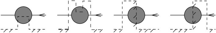
FIG. 6.: Schematic depiction of the possible ways to cut a self-energy insertion diagram.

To show that in fact the pinching pole contributions all cancel, consider the diagrams shown in Fig. 6. They differ only in the manner of cutting. Representing the blobs in the first and third diagrams by $C(k)$ and $L(k)$, respectively, the sum of the four diagrams can be written

$${\cal F}(k) = G_{\rm B}(k)C(k)G_{\rm B}(k)+\Delta_{\rm B}^{-}(k)C^{*}(k)\Delta_{\rm B}^{+}(k)$$ (80)

$${}-\Delta_{\rm B}^{-}(k)L(k)G_{\rm B}(k)-G_{\rm B}(k)L(-k)\Delta_{\rm B}^{+}(k)\;.$$

Extracting the coefficient of the pinching poles $2(k^{2}-m^{2}+i\epsilon)^{-1}(k^{2}-m^{2}-i\epsilon)^{-1}$, we find

$${\cal F}_{\hbox{pinch}}(k) = n_{\rm B}(k^{0})N_{\rm B}(k^{0})\left(C(k)+C^{*}(k)\right)$$ (82)

$${}-n_{\rm B}(k_{0})(1/2+n_{\rm B}(k_{0}))L(k)-N_{\rm B}(k_{0})(1/2+n_{\rm B}(k_{0}))L(-k)\;.$$

If ${\cal F}_{\hbox{pinch}}(k)$ were non-zero, a self-energy insertion would cause an uncontrollable divergence. Fortunately, ${\cal F}_{\hbox{pinch}}(k)$ does vanish due to the following properties of $C(k)$ and $L(k)$ [5, 7, 8, 16]

$$C(k)+C^{*}(k)=L(k)+L(-k)$$ (83)

and (84)

$$L(-k)=e^{-k^{0}\beta}\,L(k)\;.$$

The first identity (83) is the finite temperature version of the optical theorem. The second identity can be easily obtained by using $\Delta_{\rm B}^{+}(k)=e^{k^{0}\beta}\Delta_{\rm B}^{-}(k)$. Therefore, pinching poles do not occur in self-energies insertions.

The absence of pinching poles has two important consequences. First, self-energy insertions do not cause uncontrollable divergences due to the cancellation between cut and uncut self-energies. Second, the propagators connected to a self-energy do not produce thermal phase-space factors. Without this second point it would not be possible to identify the coefficients of the expansion in the $\Gamma_{\zeta}$ factors with the scattering amplitudes.

D Polarization Factors and the Overall Sign

To convert a Feynman diagram to a scattering amplitude, one needs the polarization factors for the external lines. For an external gauge boson line, a polarization vector $\epsilon_{\mu}(p,s)$ orthogonal to the incoming momentum $p$ is needed. This is provided by the substitution

$$g_{\mu\nu}\to-\sum_{s=1,2}\epsilon_{\mu}(p,s)\epsilon_{\nu}^{*}(p,s)$$ (85)

inside a Feynman diagram; this is valid due to the Ward identity. In the Feynman gauge, the gauge boson phase space factor is proportional to the metric $g_{\mu\nu}$ which then provides appropriate $\epsilon_{\mu}$’s.

For fermions, each incoming fermion (anti-fermion) line requires a factor of the Dirac spinor $u_{s}(p)$ ($\bar{v}_{s}(p)$), and each outgoing fermion (anti-fermion) line requires a factor of $\bar{u}_{s}(p)$ ($v_{s}(p)$). For the external line corresponding to the self-energy momentum, one can use the Dirac spinor identity

$${\bf 1}={1\over 2m_{F}}\sum_{s}\left(u_{s}(k)\bar{u}_{s}(k)-v_{s}(k)\bar{v}_{s}(k)\right)\;,$$ (86)

where the spinors are normalized according to Peskin and Schroeder [20]. This yields

$$\Sigma_{\rm F}(k) = {\bf 1}\Sigma_{\rm F}(k){\bf 1}$$ (87)

$$= {1\over 4m_{F}^{2}}\sum_{s}\left\{u_{s}(k)\Big{[}\bar{u}_{s}(k)\Sigma_{\rm F}(k)u_{s}(k)\Big{]}\bar{u}_{s}(k)+v_{s}(k)\Big{[}\bar{v}_{s}(k)\Sigma_{\rm F}(k)v_{s}(k)\Big{]}\bar{v}_{s}(k)\right\}\;.$$ (88)

The factor $\bar{u}_{s}(k)\Sigma_{\rm F}(k)u_{s}(k)/(2m_{F})$ then has a multiple scattering expansion in terms of spin up-up and down-down scattering amplitudes involving the particles, while the factor $\bar{v}_{s}(k)\Sigma_{\rm F}(k)v_{s}(k)/(2m_{F})$ has a multiple scattering expansion in terms of spin up-up and down-down scattering amplitudes involving the anti-particles. The mixed term vanishes since $\bar{u}(k)\gamma^{0}v(k)=\bar{v}(k)\gamma^{0}u(k)=\bar{u}(k)k^{\mu}\gamma_{\mu}v(k)=\bar{v}(k)k^{\mu}\gamma_{\mu}u(k)=0$, and the self-energy, as well as the spectral density, must have the structure

$$\Sigma_{\rm F}(k)=A(T,k)\gamma^{\mu}k_{\mu}-B(T,k)m_{F}+C(T,k)\gamma^{0}\;$$ (89)

at finite temperature.

As an example, consider the nucleon self-energy in a thermal pion medium. Considering only the strong interaction, we can regard both the pions and the nucleons as stable. The up-up component of the lowest order nucleon self-energy can then be expressed as

$$\Sigma_{T}^{++}(k) \equiv {\bar{u}_{+}(k)\Sigma_{T}(k)u_{+}(k)\over 2m_{N}}$$ (90)

$$= -{1\over 2m_{N}}\sum_{a}\int{d^{3}l_{\pi}\over(2\pi)^{3}2E_{\pi}}\,n_{B}(E_{\pi})\,{\cal T}^{++}_{N\pi_{a}\to N\pi_{a}}(k+l_{\pi}\to k+l_{\pi})$$ (91)

$$= -2\pi\sum_{a}\int{d^{3}l_{\pi}\over(2\pi)^{3}E_{\pi}}\,n_{B}(E_{\pi})\,\left({\sqrt{s}\over m_{N}}\right)f^{++}_{N\pi_{a}}(k,l_{\pi})\;,$$ (92)

where ${\cal T}^{++}_{N\pi_{a}\to N\pi_{a}}(k+l_{\pi}\to k+l_{\pi})$ is the sum of all scattering amplitudes including the cross terms. In the last line we used ${\cal T}=8\pi\sqrt{s}\,f$. This expression differs by a factor of $\sqrt{s}/m_{N}$ from that given by Eletskii and Ioffe [26]. At low temperature ($T\ll m_{N}$) and in the nucleon rest frame, their expression may be justified because the pion thermal energy is insignificant compared to the nucleon rest mass.

For internal fermion lines which are opened up and given thermal weightings we use the relation

$${}(k^{\mu}\gamma_{\mu}+m_{F})\,2\pi\,\delta(k_{0}^{2}-E_{k}^{2})=(k_{+}^{\mu}\gamma_{\mu}+m_{F})\,{2\pi\over 2E_{k}}\,\delta(k_{0}-E_{k})-(k_{-}^{\mu}\gamma_{\mu}-m_{F})\,{2\pi\over 2E_{k}}\,\delta(k_{0}+E_{k})$$ (93)

$${\hskip 56.9055pt}=\sum_{s}u_{s}(k_{+})\bar{u}_{s}(k_{+})\,{2\pi\over 2E_{k}}\,\delta(k_{0}-E_{k})-\sum_{s}v_{s}(k_{-})\bar{v}_{s}(k_{-})\,{2\pi\over 2E_{k}}\,\delta(k_{0}+E_{k})\;,$$ (94)

where $k_{\pm}=(E_{k},\pm{\bf k})$. Hence for both spin-1 gauge bosons and spin-$\frac{1}{2}$ fermions the polarization factors are all correctly accounted for.

When fermions are involved, our expansion must generate the correct overall sign of a diagram. The presence of a fermion loop in a diagram carries an additional overall factor of $(-1)$. When the fermion loop is broken this sign is carried by the thermal phase space factor, $\Gamma_{F}$ rather than the scattering amplitude. The $v\bar{v}$ part of Eq. (94) carries an additional $(-1)$ due to the exchange of the fermion legs. When a fermion line which is not a part of a fermion loop carries a thermal phase space factor, the $u\bar{u}$ term corresponds to a crossed diagram and the required factor of $(-1)$ is provided by $\Gamma_{F}$. Hence, the overall signs are also correctly accounted for in our expansion.

IV Electron Self-Energy

FIG. 7.: The one-loop electron self-energy. The curly line represents the photon.

As an example of applying the method developed here, consider the electron self-energy at temperatures $T\ll m_{e}$ obtained from the diagram of Fig. 7. At these low temperatures, we can neglect the electron thermal correction because it is suppressed by a factor of $e^{-\beta m_{e}}$. The self-energy written down for the nucleon (92) is valid for the electron if the pion is changed to a photon with the summation referring to the photon polarization:

$$\Sigma_{T}^{++}(p) = -{1\over 2m_{e}}\sum_{s=1,2}\int{d^{3}k\over(2\pi)^{3}2|{\bf k}|}\,n_{B}(|{\bf k}|)\,{\cal T}^{++}_{e\gamma\to e\gamma}(p+k\to p+k)\;.$$ (95)

After the photon polarization summation, the spin up-up component of the tree-level Compton scattering amplitude is given by (e.g. Ref. [20])

$${\cal T}^{++}_{e\gamma\to e\gamma}(p+k\to p+k) = e^{2}\bar{u}_{+}(p)\left[{\gamma^{\mu}\hbox to0.0pt{/\hss}k\gamma_{\mu}+2\hbox to0.0pt{/\hss}p\over 2p{\cdot}k+i\epsilon}+{-\gamma^{\mu}\hbox to0.0pt{/\hss}k\gamma_{\mu}+2\hbox to0.0pt{/\hss}p\over-2p{\cdot}k+i\epsilon}\right]u_{+}(p)\;.$$ (96)

In the electron rest frame, this reduces to

$${\cal T}^{++}_{e\gamma\to e\gamma}(p+k\to p+k)=-4e^{2}\left[1+\frac{2m_{e}^{2}\epsilon i}{4m_{e}^{2}|{\bf k}|^{2}+\epsilon^{2}}\right]\;.$$ (97)

The real part in the rest frame is then,

$${\rm Re}\,\Sigma_{T}^{++}(m_{e}) = {2e^{2}\over m_{e}}\int{d^{3}k\over(2\pi)^{3}2|{\bf k}|}\,n_{B}(|{\bf k}|)\,$$ (98)

$$= {e^{2}T^{2}\over 12m_{e}}={\pi\alpha T^{2}\over 3m_{e}}\;.$$ (99)

The result, of course, coincides with a previous calculation [27]. The imaginary part is

$${\rm Im}\,\Sigma_{T}^{++}(m_{e}) = \lim_{\epsilon\to 0}4e^{2}m_{e}\epsilon\int{d^{3}k\over(2\pi)^{3}2|{\bf k}|}\,\frac{n_{B}(|{\bf k}|)}{(4m_{e}^{2}|{\bf k}|^{2}+\epsilon^{2})}$$ (100)

$$= {e^{2}T\over 4\pi}=\alpha T\;.$$ (101)

This agrees with the leading term given by Henning et al. [28].

V Conclusion

In this paper, the multiple scattering expansion of the thermal correction to the retarded self-energy is presented starting from the imaginary-time formalism. The leading order term of this expansion corresponds to the often used rule that the thermal correction to the self-energy is the thermal phase-space times the scattering amplitude. Although the formal expansion can be always made, we have argued that the expansion is useful only if the minimum of $|m_{a}\pm\mu_{a}|$ is large compared to the temperature. We have also demonstrated the connection between the self-energy and the thermal part of the grand potential.

The result presented here may be used in two ways. One is to use existing calculations of scattering amplitudes to calculate the self-energy. In this way, the considerable effort usually needed to evaluate thermal correlation functions can be much reduced. The other way is simply to use experimental scattering amplitudes to calculate the self-energy. For interactions involving large coupling constants, this may be the only reliable way to calculate the thermal correction to the self-energy.

The reliable calculation of medium effects is important in analyzing data from heavy-ion collision experiments. For instance, how the $\rho$-meson behaves in-medium can greatly influence the dilepton spectrum in heavy ion collisions [1, 29]. The in-medium effect becomes even more important in future RHIC (Relativistic Heavy Ion Collider) experiments. The main goal of RHIC is to find the quark-gluon plasma. Hence, it is crucial to understand the hadronic part of the in-medium finite-temperature effect so as to separate this signal from that of the long-sought quark-gluon plasma. Even though a full theory of hadron scattering is lacking, there is a considerable amount of data on scattering cross-sections accumulated in the past decades. Utilizing those data we may at least phenomenologically separate a truly hadronic effect from the effect of a new state of matter.

A Euclidean Propagators

1 Bosonic Propagator With Chemical Potential

When the chemical potential is non-zero, we must at least deal with a complex field. The effective Hamiltonian is

$$\hat{K}\equiv\hat{H}-\sum_{a}\mu_{a}\hat{Q}_{a}\;.$$ (A1)

For notational convenience we suppress spatial indices in this section.

The spectral density for the propagator is defined to be [11]

$$\rho_{\rm B}(\omega) = \int dt\,e^{i\omega t}\,\langle[\phi(t),\phi^{\dagger}]\rangle$$ (A2)

$$= \sum_{m,n}\int dt\,e^{i\omega t}\,\left(e^{-\beta K_{m}}e^{it(K_{m}-K_{n})}\phi_{mn}\phi^{\dagger}_{nm}-e^{-\beta K_{n}}\phi^{\dagger}_{nm}e^{it(K_{m}-K_{n})}\phi_{mn}\right)$$ (A3)

$$= \sum_{m,n}2\pi\delta(\omega+K_{m}-K_{n})\,\left(e^{-\beta K_{m}}-e^{-\beta K_{n}}\right)\phi_{mn}\phi^{\dagger}_{nm}$$ (A4)

$$= \left(1-e^{-\beta\omega}\right)\sum_{m,n}2\pi\delta(\omega+K_{m}-K_{n})\,\phi_{mn}\phi^{\dagger}_{nm}e^{-\beta K_{m}}\;.$$ (A5)

The Euclidean propagator is given by

$$G_{\rm B}(\tau) = \langle{\cal T}\phi(\tau)\phi^{\dagger}(0)\rangle$$ (A6)

$$= \theta(\tau){\rm Tr}\left(e^{-\beta\hat{K}}e^{\tau\hat{K}}\phi e^{-\tau\hat{K}}\phi^{\dagger}\right)+\theta(-\tau){\rm Tr}\left(e^{-\beta\hat{K}}\phi^{\dagger}e^{\tau\hat{K}}\phi e^{-\tau\hat{K}}\right)$$ (A7)

$$= \int{d\omega\over 2\pi}\,\left(e^{-\omega\tau}[1+n_{\rm B}(\omega)]\,\rho_{B}(\omega)\theta(\tau)+e^{-\omega\tau}n_{\rm B}(\omega)\,\rho_{B}(\omega)\theta(-\tau)\right)$$ (A8)

$$= \int{d\omega\over 2\pi}\,[1+n_{\rm B}(\omega)]\left(e^{-\omega\tau}\,\rho_{\rm B}^{+}(\omega)\,\theta(\tau)+e^{\omega\tau}\,\rho_{\rm B}^{-}(\omega)\,\theta(-\tau)\right)\;,$$ (A9)

where we used

$$n_{\rm B}(-\omega)=-[1+n_{\rm B}(\omega)]\;,$$ (A10)

and defined

$$\rho_{\rm B}^{+}(\omega)\equiv\rho_{\rm B}(\omega)\quad;\quad\rho_{\rm B}^{-}(\omega)\equiv-\rho_{\rm B}(-\omega)\;.$$ (A11)

To find $\rho^{+}_{\rm B}(\omega)$, use [11]

$$G_{\rm B}(i\nu_{B},{\bf k})={1\over E_{k}^{2}-(i\nu_{B}+\mu)^{2}}=\int{d\omega\over 2\pi}\,{\rho^{+}_{\rm B}(\omega,{\bf k})\over\omega-i\nu_{B}}\;,$$ (A12)

with $E_{k}=\sqrt{{\bf k}^{2}+m^{2}}$, and take the discontinuity across the real axis to get

$$\rho^{+}_{\rm B}(\omega,{\bf k}) = {\rm sign}(\omega+\mu)\,2\pi\,\delta\left((\omega+\mu)^{2}-E_{k}^{2}\right)$$ (A13)

and

$$\rho^{-}_{\rm B}(\omega,{\bf k}) = -\rho^{+}_{\rm B}(-\omega,{\bf k})={\rm sign}(\omega-\mu)\,2\pi\,\delta\left((\omega-\mu)^{2}-E_{k}^{2}\right)\;.$$ (A14)

2 Fermionic Propagators with Chemical Potential

The spectral density for the fermion propagator is defined to be

$$\rho_{\rm F}(\omega) = \int dt\,e^{i\omega t}\,\langle\{\psi(t),\bar{\psi}\}\rangle$$ (A15)

$$= \sum_{m,n}2\pi\delta(\omega+K_{m}-K_{n})\,\left(e^{-\beta K_{m}}+e^{-\beta K_{n}}\right)\psi_{mn}\bar{\psi}_{nm}$$ (A16)

$$= \left(1+e^{-\beta\omega}\right)\sum_{m,n}2\pi\delta(\omega+K_{m}-K_{n})\,\psi_{mn}\bar{\psi}_{nm}e^{-\beta K_{m}}\;,$$ (A17)

where the brace denotes an anticommutator and we used the fact that matrix elements such as $\psi_{mn}$ are c-numbers.

The Euclidean propagator is given by

$$G_{\rm F}(\tau) = \langle{\cal T}\psi(\tau)\bar{\psi}(0)\rangle$$ (A18)

$$= \theta(\tau){\rm Tr}\left(e^{-\beta\hat{K}}e^{\tau\hat{K}}\psi e^{-\tau\hat{K}}\bar{\psi}\right)-\theta(-\tau){\rm Tr}\left(e^{-\beta\hat{K}}\bar{\psi}e^{\tau\hat{K}}\psi e^{-\tau\hat{K}}\right)$$ (A19)

$$= \int{d\omega\over 2\pi}\,\left(e^{-\omega\tau}[1-n_{\rm F}(\omega)]\,\rho^{+}_{\rm F}(\omega)\theta(\tau)-e^{-\omega\tau}n_{\rm F}(\omega)\,\rho^{+}_{\rm F}(\omega)\theta(-\tau)\right)$$ (A20)

$$= \int{d\omega\over 2\pi}\,[1-n_{\rm F}(\omega)]\left(e^{-\omega\tau}\,\rho_{\rm F}^{+}(\omega)\theta(\tau)+e^{\omega\tau}\,\rho_{\rm F}^{-}(\omega)\theta(-\tau)\right)\;,$$ (A21)

where the change of variable $\omega\to-\omega$ was made for the second term and we used

$$n_{\rm F}(-\omega)={1\over e^{-\omega\beta}+1}=1-n_{\rm F}(\omega)\;.$$ (A22)

Also, we defined

$$\rho_{\rm F}^{+}(\omega)\equiv\rho_{\rm F}(\omega)\quad;\quad\rho_{\rm F}^{-}(\omega)\equiv-\rho_{\rm F}(-\omega)\;.$$ (A23)

Hence, for both bosons and fermions we have

$$G_{\zeta}(\tau)=\int{d\omega\over 2\pi}\,N_{\zeta}(\omega)\left(e^{-\omega\tau}\,\rho_{\zeta}^{+}(\omega)\theta(\tau)+e^{\omega\tau}\,\rho_{\zeta}^{-}(\omega)\theta(-\tau)\right)\;,$$ (A24)

with

$$\rho_{\zeta}^{+}(\omega) = -\rho_{\zeta}^{-}(-\omega)\;,$$ (A25)

and

$$N_{\zeta}(\omega) = 1+(-1)^{\zeta}n_{\zeta}(\omega)=\theta(\omega)+(-1)^{\zeta}{\rm sign}(\omega)n_{\zeta}(|\omega|)\;,$$ (A26)

where

$$(-1)^{\rm B}\equiv 1\ \ \hbox{and}\ \ (-1)^{\rm F}\equiv-1\;.$$ (A27)

To find $\rho^{+}_{\rm F}(\omega)$, start from the Euclidean propagator

$$G_{\rm F}(\nu_{\rm F},{\bf p})={i\left(\nu_{\rm F}-i\mu\right)\gamma^{0}-{\bf p}{\cdot}\hbox{\boldmath{$\gamma$}}+m\over(\nu_{\rm F}-i\mu)^{2}+E_{p}^{2}}=\int{d\omega\over 2\pi}\,{\rho^{+}_{\rm F}(\omega,{\bf k})\over\omega-i\nu_{F}}\;,$$ (A28)

with $E_{p}=\sqrt{{\bf p}^{2}+m^{2}}$, and take the discontinuity across the real axis to get

$$\rho_{\rm F}^{+}(\omega,{\bf p})=\left((\omega+\mu)\gamma^{0}-{\bf p}{\cdot}\hbox{\boldmath{$\gamma$}}+m\right){\rm sign}(\omega+\mu)\,2\pi\delta((\omega+\mu)^{2}-E_{p}^{2})\;.$$ (A29)

B Real Time Propagators

For both bosons and fermions the real time version of Eq. (A24) is

$$G_{\zeta}(t) = \int{d\omega\over 2\pi}\,N_{\zeta}(\omega)\left(e^{-i\omega t}\,\rho_{\zeta}^{+}(\omega)\,\theta(t)+e^{i\omega t}\,\rho_{\zeta}^{-}(\omega)\,\theta(-t)\right)\;.$$ (B1)

The Fourier transform yields the momentum space propagator

$$G_{\zeta}(k) = \int{d\omega\over 2\pi}\,N_{\zeta}(\omega)\left(\int_{0}^{\infty}dt\,e^{ik^{0}t-\epsilon t}e^{-i\omega t}\,\rho_{\zeta}^{+}(\omega)+\int_{-\infty}^{0}dt\,e^{ik^{0}t+\epsilon t}e^{i\omega t}\,\rho_{\zeta}^{-}(\omega)\right)$$ (B2)

$$= \int{d\omega\over 2\pi}\,[\theta(\omega)+(-1)^{\zeta}{\rm sign}(\omega)n_{\zeta}(|\omega|)]\left({\rho_{\zeta}^{+}(\omega)\over\epsilon+i(\omega-k^{0})}+{\rho_{\zeta}^{-}(\omega)\over\epsilon+i(\omega+k^{0})}\right)\;,$$ (B3)

using Eq. (A26). The propagator has two terms. The first corresponds to the zero temperature case

$$G_{\zeta}^{0}(k)=\int{d\omega\over 2\pi}\,\theta(\omega)\left({\rho_{\zeta}^{+}(\omega)\over\epsilon+i(\omega-k^{0})}+{\rho_{\zeta}^{-}(\omega)\over\epsilon+i(\omega+k^{0})}\right)\;,$$ (B4)

which yields the standard Minkowski propagators given in the text. The second term corresponds to the finite temperature phase space factor

$$\Gamma_{\zeta}(k) = (-1)^{\zeta}\int{d\omega\over 2\pi}\,{\rm sign}(\omega)n_{\zeta}(|\omega|)\left({\rho_{\zeta}^{+}(\omega)\over\epsilon+i(\omega-k^{0})}+{\rho_{\zeta}^{-}(\omega)\over\epsilon+i(\omega+k^{0})}\right)$$ (B5)

$$= (-1)^{\zeta}{\rm sign}(k^{0})n_{\zeta}(|k^{0}|)\rho_{\zeta}^{+}(k)\;,$$ (B6)

where we used $\rho_{\zeta}^{-}(\omega)=-\rho_{\zeta}^{+}(-\omega)$.

Cut propagators can also be decomposed into zero and non-zero temperature parts. The cut propagator for a particle is

$$\Delta_{\zeta}^{+}(k)\equiv N_{\zeta}(k^{0})\rho_{\zeta}^{+}(k)=\theta(k^{0})\rho_{\zeta}^{+}(k)+(-1)^{\zeta}{\rm sign}(k^{0})n_{\zeta}(|k^{0}|)\,\rho_{\zeta}^{+}(k)\;.$$ (B7)

Letting the momentum and frequency follow the charge, we get the cut propagator for an anti-particle $N_{\zeta}(k^{0})\rho_{\zeta}^{-}(k)\to N_{\zeta}(-k^{0})\rho_{\zeta}^{-}(-k)$ which is

$$\Delta_{\zeta}^{-}(k)\equiv N_{\zeta}(-k^{0})\rho_{\zeta}^{-}(-k) = (-1)^{\zeta}\,n_{\zeta}(k^{0})\,\rho_{\zeta}^{+}(k)$$ (B8)

$$= -\theta(-k^{0})\rho_{\zeta}^{+}(k)+(-1)^{\zeta}\,{\rm sign}(k^{0})\,n_{\zeta}(|k^{0}|)\,\rho_{\zeta}^{+}(k)\;,$$ (B9)

using

$$n_{\zeta}(k^{0})=-(-1)^{\zeta}\theta(-k^{0})+{\rm sign}(k^{0})n_{\zeta}(|k^{0}|)\;.$$ (B10)

We also note that $\Delta_{\zeta}^{+}(k)=(-1)^{\zeta}e^{\beta k_{0}}\Delta_{\zeta}^{-}(k)$.

C Derivative Couplings

For the time derivative of the propagator in Eq. (A24) we have

$${\partial\over\partial\tau}G_{\zeta}(\tau,{\bf k}) = \int{d\omega\over 2\pi}\,N_{\zeta}(\omega)\,\left(-\omega\rho_{\zeta}^{+}(\omega,{\bf k})\,e^{-\omega\tau}\,\theta(\tau)\,+\omega\rho_{\zeta}^{-}(\omega,{\bf k})\,e^{\omega\tau}\,\theta(-\tau)\,\right)$$ (C2)

$${}+\int{d\omega\over 2\pi}\,N_{\zeta}(\omega)\,\left(\rho_{\zeta}^{+}(\omega,{\bf k})-\rho_{\zeta}^{-}(\omega,{\bf k})\right)\delta(\tau)$$

$$= \int{d\omega\over 2\pi}\,N_{\zeta}(\omega)\,\left(-\omega\rho_{\zeta}^{+}(\omega,{\bf k})\,e^{-\omega\tau}\,\theta(\tau)\,+\omega\rho_{\zeta}^{-}(\omega,{\bf k})\,e^{\omega\tau}\,\theta(-\tau)\,\right)$$ (C4)

$${}+\int{d\omega\over 2\pi}\,\rho_{\zeta}^{+}(\omega,{\bf k})\delta(\tau)\;.$$

Thus the spectral density for the time derivative of the propagator is $-\omega\rho_{\zeta}^{+}(\omega,{\bf k})$ and there is also a $\delta(\tau)$ term. The latter vanishes for bosons since $\int d\omega\,\rho_{\rm B}^{+}(\omega,{\bf k})=0$. In general, we can say

$$\partial_{\tau}^{r}G_{\zeta}(\tau,{\bf k})=\tilde{G}_{\xi}(\tau,{\bf k})+\sum_{l=0}^{r-1}\delta^{(l)}(\tau)F_{l}({\bf k})\;,$$ (C5)

where the label $\xi$ includes both $\zeta$ and the number of derivatives $r$ so that $\tilde{G}_{\xi}$ has the spectral density $(-\omega)^{r}\rho_{\zeta}^{+}$. In the second term of (C5) $\delta^{(l)}(\tau)=\partial_{\tau}^{l}\delta(\tau)$ and the sum does not contribute for $r=0$. Then, after all the $\delta$-functions in Eq. (C5) are integrated over, we have

$$C_{N+1}^{(\Gamma)}(\{{\bf q}_{l},i\nu_{l}\})$$ (C6)

$$= \int_{0}^{\beta}\prod_{i=0}^{V}d\tau_{i}\exp\left(i\sum_{l=0}^{N}\nu_{l}\tau_{l}\right)\,\int\prod_{L\in\Gamma}{d^{3}k_{L}\over(2\pi)^{3}}\,A_{0}\left(\{{\bf k}_{\alpha}\}\right)\,\prod_{\alpha\in\Gamma}{}\tilde{G}_{\xi_{\alpha}}(\tau^{\alpha}_{a}-\tau^{\alpha}_{b})$$ (C10)

$${}+\sum_{r}\int_{0}^{\beta}\prod_{i\neq r}^{V}d\tau_{i}\exp\left(i\sum_{l\neq r}^{N}\bar{\nu}_{l}\tau_{l}\right)\,\int\prod_{L\in\Gamma}{d^{3}k_{L}\over(2\pi)^{3}}\,A_{1}\left(\{{\bf k}_{\alpha},i\nu_{r}\}\right)\,\prod_{\alpha\in\Gamma^{\prime}}{}\tilde{G}_{\xi_{\alpha}}(\tau^{\alpha}_{a}-\tau^{\alpha}_{b})$$

$${}+\sum_{q,r}\int_{0}^{\beta}\prod_{i\neq r,q}^{V}d\tau_{i}\exp\left(i\sum_{l\neq r,q}^{N}\bar{\bar{\nu}}_{l}\tau_{l}\right)\,\int\prod_{L\in\Gamma}{d^{3}k_{L}\over(2\pi)^{3}}\,A_{2}\left(\{{\bf k}_{\alpha},i\nu_{r},i\nu_{q}\}\right)\,\prod_{\alpha\in\Gamma^{\prime\prime}}{}\tilde{G}_{\xi_{\alpha}}(\tau^{\alpha}_{a}-\tau^{\alpha}_{b})$$

$${}+\cdots\;,$$

where in $\Gamma^{\prime}$ a pair of vertices refer to the same time, in $\Gamma^{\prime\prime}$ two pairs of vertices refer to the same times, and so on. The bars over the $\nu_{l}$ indicates that some of them are now combinations of the original $\nu_{l}$’s.

If a total of $n$ derivatives is contained in the expression for the diagram $\Gamma$, then performing the time integrals we have

$${C}_{N{+}1}^{(\Gamma)}(\{{\bf q}_{l},i\nu_{l}\})=\sum_{r=0}^{n}\sum_{{\Gamma_{\sigma}^{r}}\subset\Gamma_{r}}\;C_{N+1}^{(\Gamma_{\sigma}^{r})}(\{{\bf q}_{l},i\nu_{l}\})$$ (C11)

where

$$C_{N+1}^{(\Gamma_{\sigma}^{r})}(\{{\bf q}_{l},i\nu_{l}\})$$ (C12)

$$= \int\prod_{L\in\Gamma}{d^{3}k_{L}\over(2\pi)^{3}}\,\prod_{\alpha\in\Gamma_{r}}\left(\int{d\omega_{\alpha}\over 2\pi}\,N_{\zeta_{\alpha}}(\omega_{\alpha})\,\rho_{\xi_{\alpha}}^{s_{\sigma}}(k_{\alpha})\right)\,A_{r}\left(\{{\bf k}_{\alpha}\},\{i\nu_{l}\}\right)\,\prod_{{\hbox{{\rm intervals}}\atop\hbox{$\scriptstyle{V-r\geq j\geq 1}$}}}\Bigl{(}\Lambda_{j}^{\sigma}-i\nu_{j}^{\sigma}\Bigr{)}^{-1}\;.$$ (C13)

(C14)

We know that in the $\beta\to\infty$ limit, the frequency denominators we get from Eq. (C14) must add up to make the Wick rotated $\partial_{t}^{r}G_{\zeta}(t)$. That is, the coefficients $A_{r}$ must be such that if we change $N\to\theta$, $i\nu_{l}\to q_{l}^{0}$ and add $-i\epsilon$ to $\Lambda_{j}^{\sigma}$ in Eq. (C14), we get the zero temperature $N+1$-point function:

$${C}_{N{+}1}^{(\Gamma)}(\{{\bf q}_{l},i\nu_{l}\})\rightarrow{D}_{N{+}1}^{(\Gamma)}(\{q_{l}\})=i^{V}\int\prod_{L\in\Gamma}{d^{4}k_{L}\over(2\pi)^{4}}\,A(\{k_{L}\})\prod_{\alpha\in\Gamma}G_{\zeta_{\alpha}}(k_{\alpha})\;,$$ (C15)

as in Eq. (37). Arguments similar to those in Subsec. II B can be applied to cut diagrams so that summing the time-ordered diagrams on the unshaded side leads to the usual Feynman rules, while for the shaded side complex conjugate Feynman rules apply. Thus the multiple scattering expansion of the self-energy in Sec. 3 is also applicable when derivative couplings are present.

D The Thermodynamic Potential

Here we consider the multiple scattering expansion of the thermodynamic grand potential defined by

$${\Omega\over V}\equiv-{1\over\beta V}\,\ln Z$$ (D1)

where $Z$ is the partition function and $V$ is the volume. In the imaginary-time formalism, the thermodynamic potential is the sum of all connected “vacuum” graphs. Analytic continuation of such a result may at first appear to be a poorly defined concept since there are no external frequencies to start with. Nevertheless, it is possible to consider the vacuum graphs as the zero frequency limit of the $N$-point functions [30] and, further, it is sufficient to consider retarded correlation functions due to the reality of the thermodynamic potential.

To calculate $\Omega$, we regard the $\hat{\varphi}$ in Eq. (26) as “external” interaction vertices which will contain several fields. The retarded functions then consist entirely of all possible interaction vertices and there are zero external frequencies and momenta entering or leaving the diagram. Eq. (31) can then be written

$${R}_{N{+}1}^{(\Gamma_{v})}(0) = \displaystyle\sum_{{\Gamma_{\sigma}}\subset\Gamma}\;\int\prod_{L\in\Gamma}{d^{3}k_{L}\over(2\pi)^{3}}\,\prod_{\alpha\in\Gamma}\left(\int{d\omega_{\alpha}\over 2\pi}\,N_{\zeta_{\alpha}}(\omega_{\alpha})\,\rho_{\zeta_{\alpha}}^{s_{\sigma}}(k_{\alpha})\right)A_{V+1}^{N+1}$$ (D3)

$$\qquad{}\times\prod_{{\hbox{{\rm intervals}}\atop\hbox{$\scriptstyle{V\geq j\geq v+1}$}}}\Bigl{(}\Lambda_{j}^{\sigma}+i\epsilon\Bigr{)}^{-1}\prod_{{\hbox{{\rm intervals}}\atop\hbox{$\scriptstyle{v\geq j^{\prime}\geq 1}$}}}\Bigl{(}\Lambda_{j^{\prime}}^{\sigma}-i\epsilon\Bigr{)}^{-1}\;.$$

Here the fixed vertex $v$ is arbitrarily chosen for each diagram. Instead of the identity (38), we use

$${1\over\Lambda_{j}^{\sigma}+i\epsilon}={1\over\Lambda_{j}^{\sigma}-i\epsilon}-2\pi i\delta(\Lambda_{j}^{\sigma})\;,$$ (D4)

to get

$${R}_{N{+}1}^{(\Gamma_{v})}(0) = \displaystyle\sum_{{\Gamma_{\sigma}}\subset\Gamma}\;\int\prod_{L\in\Gamma}{d^{3}k_{L}\over(2\pi)^{3}}\,\prod_{\alpha\in\Gamma}\left(\int{d\omega_{\alpha}\over 2\pi}\,N_{\zeta_{\alpha}}(\omega_{\alpha})\,\rho_{\zeta_{\alpha}}^{s_{\sigma}}(k_{\alpha})\right)A_{V+1}^{N+1}$$ (D9)

$$\qquad{}\times\Bigg{[}\prod_{{\hbox{{\rm intervals}}\atop\hbox{$\scriptstyle{V\geq j^{\prime}\geq 1}$}}}\Bigl{(}\Lambda_{j^{\prime}}^{\sigma}-i\epsilon\Bigr{)}^{-1}$$

$$\qquad\quad{}+(-i)\sum_{j=v+1}^{V}\,2\pi\delta(\Lambda_{j}^{\sigma})\prod_{{\hbox{$\scriptstyle{V\geq k\geq 1}$}\atop\hbox{$\scriptstyle{k\neq j}$}}}\Bigl{(}\Lambda_{k}^{\sigma}-i\epsilon\Bigr{)}^{-1}$$

$$\qquad\quad{}+(-i)^{2}\sum_{j,k=v+1}^{V}\,2\pi\delta(\Lambda_{j}^{\sigma})2\pi\delta(\Lambda_{k}^{\sigma})\prod_{{\hbox{$\scriptstyle{V\geq l\geq 1}$}\atop\hbox{$\scriptstyle{l\neq j,k}$}}}\Bigl{(}\Lambda_{k}^{\sigma}-i\epsilon\Bigr{)}^{-1}$$

$$\qquad\quad{}+\ldots+(-i)^{V-v}\prod_{{\hbox{{\rm intervals}}\atop\hbox{$\scriptstyle{V\geq j\geq v+1}$}}}2\pi\delta(\Lambda_{j}^{\sigma})\prod_{{\hbox{$\scriptstyle{v\geq k\geq 1}$}}}\Bigl{(}\Lambda_{k}^{\sigma}-i\epsilon\Bigr{)}^{-1}\Bigg{]}\;.$$

In this way the denominators contain only $-i\epsilon$ and consequently, after summing over all time orderings $\sigma$, the result can be expressed entirely in terms of $G_{\zeta}(k)$ and $\Delta_{\zeta}^{\pm}(k)$, i.e. the complex conjugate propagator $G_{\zeta}^{*}(k)$ does not occur. The price paid is the appearance of multiple cuts since each of the $\delta$-functions in Eq. (D9) represents a cut. So the result of the time ordering summation will yield uncut diagrams plus those with a sequence of cuts illustrated in Fig. 8.

FIG. 8.: Diagrams for the thermodynamic potential. The dashed line indicates a cut.

The blobs in these diagrams involve the propagators $G_{\zeta}(k)$, while the cut lines require $\Delta_{\zeta}^{\pm}$ according to the direction of the momentum, as before.

Following the same procedure as before, we can now expand the diagrams in the number of thermal phase space factors $\Gamma_{\zeta}$. The contribution of the first term in Eq. (D9) to the thermal part of $\Omega$ is

$${\Omega_{T}^{(1)}\over V}=-\sum_{n\geq 2,\sigma}{1\over S_{\{l_{i}^{\sigma}\}}}\int\prod_{i=1}^{n}d\Gamma_{i}^{\sigma}\,\langle\{l_{i}^{\sigma}\}|{\cal T}|\{l_{i}^{\sigma}\}\rangle_{\hbox{conn}}\;,$$ (D10)

where we have excluded diagrams with a single thermal weighting since we assume that the physical masses of the particles are used in the propagators. The contribution of diagrams with $(m-1)$ cuts is

$${\Omega_{T}^{(m)}\over V}=-\sum_{n\geq 2,\sigma}{1\over S_{\{l_{i}^{\sigma}\}}}\int\prod_{i=1}^{n}d\Gamma_{i}^{\sigma}\,\langle\{l_{i}^{\sigma}\}|{\cal T}_{v}(-i{\cal T})^{m-1}|\{l_{i}^{\sigma}\}\rangle_{\hbox{conn}}\;.$$ (D11)

Here ${\cal T}_{v}$ contains the arbitarily-chosen fixed vertex, $v$. If, however, we remove this restriction and allow $v$ to lie in any of the ${\cal T}$ matrices, while compensating for the multiple counting, we obtain

$${\Omega_{T}^{(m)}\over V}=-i\sum_{n\geq 2,\sigma}{1\over S_{\{l_{i}^{\sigma}\}}}\int\prod_{i=1}^{n}d\Gamma_{i}^{\sigma}\,{1\over m}\langle\{l_{i}^{\sigma}\}|(-i{\cal T})^{m}|\{l_{i}^{\sigma}\}\rangle_{\hbox{conn}}\;.$$ (D12)

Summing over the number of cuts, we then have

$${\Omega_{T}\over V}=\sum_{m=1}^{\infty}{\Omega_{T}^{(m)}\over V}=i\sum_{n\geq 2,\sigma}{1\over S_{\{l_{i}^{\sigma}\}}}\int\prod_{i=1}^{n-1}d\Gamma_{i}^{\sigma}\,\langle\{l_{i}^{\sigma}\}|\ln(1+i{\cal T})|\{l_{i}^{\sigma}\}\rangle_{\hbox{conn}}\;.$$ (D13)

This is the expression given in Eq. (73) and, as we remarked, it agrees with the result Norton [23] obtained using a different approach. This in turn is equivalent to the expression obtained long ago by Dashen, Ma and Bernstein [21] from a non-relativistic analysis.

REFERENCES

• [1] E.V. Shuryak, Collective Interaction of Mesons in Hot Hadronic Matter, Nucl. Phys. A. 533, 761 (1991).
• [2] N. Ashida, H. Nakkagawa, A. Niegawa, and H. Yokota, Evaluating Finite-Temperature Reaction Rate, Ann. Phys. (NY) 215, 315 (1992).
• [3] M. Kacir and I. Zahed, Nucleons at Finite Temperature, Phys. Rev. D 54, 5536 (1996).
• [4] H. Leutwyler and A.V. Smilga, Nucleons at Finite Temperature, Nucl. Phys. B 342, 302 (1990).
• [5] R.L. Kobes and G.W. Semenoff, Discontinuity of Green Functions in Field Theory at Finite Temperature and Density (I), (II) Nucl. Phys. B 260, 714 (1985); B 272, 329 (1986).
• [6] A.J. Niemi and G.W. Semenoff, Finite Temperature Quantum Field Theory in Minkowski Space, Ann. of Phys. (NY) 152, 105 (1984).
• [7] R. Kobes, Retarded Functions, Dispersion Relations, and Cutkosky Rules at Zero and Finite Temperature, Phys. Rev. D 43, 1269 (1991).
• [8] R. Kobes, Correspondence between Imaginary-Time and Real-Time Finite-Temperature Field Theory, Phys. Rev. D 42, 562 (1990).
• [9] T.S. Evans, N-Point Finite Temperature Expectation Values at Real Times, Nucl. Phys. B 374, 340 (1992).
• [10] For example, see J.I. Kapusta, Finite Temperature Field Theory (Cambridge University Press, Cambridge, England, 1989) and references therein.
• [11] For example, see A.L. Fetter and J.D. Walecka, Quantum Theory of Many Particle Systems (McGraw Hill, New York, 1971).
• [12] S. Jeon, Computing Spectral Densities in Finite Temperature Field Theories, Phys. Rev. D 47, 4568 (1993).
• [13] R. Mills, Propagators for Many-Particle Systems (Gordon and Breach, New York, 1969).
• [14] G. Baym and A.M. Sessler, Perturbation-Theory Rules for Computing the Self-Energy Operator in Quantum Statistical Mechanics, Phys. Rev. 131, 2345 (1963).
• [15] H.A. Weldon, Simple Rules for Discontinuities in Finite-Temperature Field Theory, Phys. Rev. D 28, 2007 (1983).
• [16] S. Jeon, Hydrodynamic Transport Coefficients in Relativistic Scalar Field Theory, Phys. Rev. D 52, 3591 (1995).
• [17] R. Baier and A. Niegawa, Analytic Continuation of Thermal N-Point Functions from Imaginary- to Real-Energies, Phys. Rev. D 49, 4107 (1994).
• [18] N. P. Landsman and Ch. G. van Weert, Real- and Imaginary-Time Field Theory at Finite Temperature and Density, Phys. Rep. 145, 141 (1987).
• [19] H. Lehmann, K. Symanzik and W. Zimmermann, On the Formulation of Quantized Field Theories - II, Nuovo Cimento VI, 319 (1957).
• [20] M.E. Peskin and D.V. Schroeder, An Introduction to Quantum Field Theory (Addision-Wesley, Reading, Massachusetts, 1995).
• [21] R. Dashen, S. Ma and H.J. Bernstein, S-Matrix Formulation of Statistical Mechanics, Phys. Rev. 187, 345 (1969).
• [22] G. t’Hooft and M. Veltman, Diagrammar, CERN Yellow Report 73-9 (1973), unpublished.
• [23] R.E. Norton, Elementary Particle Scattering and Statistical Quasi-particles in Quantum Statistical Mechanics, Ann. Phys. 170, 18 (1986).
• [24] For example, see C. Itzykson and J-B. Zuber, Quantum Field Theory (McGraw-Hill, New York, 1980).
• [25] For example, see J. Mathews and R.L. Walker, Mathematical Methods of Physics (Addison-Wesley, Redwood City, California, 1964).
• [26] V.L. Eletskii and B.L. Ioffe, On the Thermal Mass Shift Of Nucleons, Phys. Lett. B 401, 327 (1997).
• [27] J.F. Donoghue and B.R. Holstein, Renormalization and Radiative Corrections at Finite Temperature, Phys. Rev. D 28, 340 (1983); 29, 3004(E) (1983).
• [28] P.A. Henning, R. Sollacher and H. Weigert, Fermion Damping Rate in a Hot Medium, hep-ph/9409280, unpublished.
• [29] W. Cassing, W. Ehehalt and C.M. Ko, Dilepton Production at SPS Energies, Phys. Lett. B 363, 35 (1995).
• [30] T.S. Evans, Thermal Bosonic Green Functions Near Zero Energy, Can. J. Phys. 71, 241 (1993).