1 Expansion of three-point functions in terms of external momenta squared

Taylor series expansions in terms of one external momentum squared, $q^{2}$ say, were considered in [1], Padé approximants were introduced in [2] and in Ref. [3] it was demonstrated that this approach can be used to calculate Feynman diagrams on their cut by analytic continuation. The Taylor coefficients are expressed in terms of “bubble diagrams”, i.e. diagrams with external momenta equal zero, which makes their evaluation relatively easy. In the case under consideration we have two independent external momenta in $d=4-2\varepsilon$ dimensions. The general expansion of (any loop) scalar 3-point function with its momentum space representation $C(p_{1},p_{2})$ can be written as

$$C(p_{1},p_{2})=\sum^{\infty}_{l,m,n=0}a_{lmn}(p^{2}_{1})^{l}(p^{2}_{2})^{m}(p_{1}p_{2})^{n}$$ (1)

where the coefficients $a_{lmn}$ are to be determined from the given diagram.

For many applications it suffices to confine to the case $p^{2}_{1}=p^{2}_{2}=0$, which is e.g. physically realized in the case of the Higgs decay into two photons ($H\to\gamma\gamma$) with $p_{1}$ and $p_{2}$ the momenta of the photons. In this case only the coefficients $a_{00n}$ are needed.

In the two-loop case we consider the scalar integral ($k_{3}=k_{1}-k_{2}$, see also Fig. 1)

$$\begin{array}[]{l}C(m_{1},\cdots,m_{6};p_{1},p_{2})=\\ \\ \frac{1}{(i\pi^{2})^{2}}\int\frac{d^{4}k_{1}d^{4}k_{2}}{((k_{1}+p_{1})^{2}-m^{2}_{1})((k_{1}+p_{2})^{2}-m^{2}_{2})((k_{2}+p_{1})^{2}-m^{2}_{3})((k_{t}+p_{2})^{2}-m^{2}_{4})(k^{2}_{2}-m^{2}_{5})(k^{2}_{3}-m^{2}_{6})}.\end{array}$$ (5)

$k_{t}$ in line 4 (with mass $m_{4}$) depends on the topology: for the planar diagram we have $k_{t}=k_{2}$ while for the non-planar we have $k_{t}=k_{3}$.

Figure 1: Planar and non-planar scalar vertex diagrams and their kinematics

With obvious abbreviations for the scalar propagators: $c_{i}$ the $i^{th}$ scalar propagator of (5) with $p_{1}=p_{2}=0$, we can quite generally write for the $n^{th}$ Taylor coefficient [4]:

$$(i\pi^{2})^{2}a_{00n}=\frac{2^{n}}{n+1}\int d^{4}k_{1}d^{4}k_{2}F_{n}\cdot\frac{1}{c_{1}~{}c_{2}~{}c_{3}~{}c_{4}~{}c_{5}~{}c_{6}}.$$ (6)

The numerator $F_{n}$ can be written as

$$F_{n}=\sum^{n}_{\nu=0}c_{1}^{-(n-\nu)}c_{3}^{-\nu}\sum^{n}_{\nu^{\prime}=0}c_{2}^{-(n-\nu^{\prime})}c_{4}^{-\nu^{\prime}}\cdot A^{n}_{\nu\nu^{\prime}}(k_{1},k_{2},k_{t})\ .$$ (7)

For the planar diagram ($k_{t}=k_{2}$) we have

$$A^{n}_{\nu\nu^{\prime}}(k_{1},k_{2})=\sum_{\mu=\max(0,\nu+\nu^{\prime}-n)}^{\left[\frac{\nu+\nu^{\prime}}{2}\right]}a^{n\mu}_{\nu\nu^{\prime}}(k^{2}_{1})^{n-(\nu+\nu^{\prime})+\mu}(k^{2}_{2})^{\mu}(k_{1}~{}k_{2})^{\nu+\nu^{\prime}-2\mu}.$$ (8)

The coefficients $a^{n\mu}_{\nu\nu^{\prime}}$ are mass independent and have been calculated with FORM up to order ${\varepsilon}^{2}$ ($d=4-2\varepsilon$) and stored for the first 30 Taylor coefficients, i.e. they are given in terms of rational numbers.

Finally all remaining integrals can be reduced by recursion [5] to bubble-integrals of the type

$$V_{\alpha\beta\gamma}(\{m\})=\int\frac{d^{d}k_{1}d^{d}k_{2}}{(k_{1}^{2}-m_{1}^{2})^{\alpha}(k_{2}^{2}-m_{2}^{2})^{\beta}((k_{1}-k_{2})^{2}-m_{3}^{2})^{\gamma}},$$ (9)

or to factorizing one-loop integrals.The genuine two-loop bubble integrals are reduced by means of recurrence relations to $V_{111}(\{m\})$. This can be done numerically for the arbitrary mass case or also analytically for special cases like e.g. only one non-zero mass. For details see [4],[5]. To perform the recursion numerically, it is important to use the multiple precision FORTRAN by D.Bailey ([6]) since tremendeous cancellations occur in this case.

We have presented one approach for the calculation of the Taylor expansion of Feynman diagrams in some detail, others were worked out in Refs. [7],[8]. The latter one is particularly suited for programming in terms of a formulae manipulating language like FORM.

2 The method of analytic continuation

We assume the Taylor expansion of a scalar diagram to be given in the form $C(p_{1},p_{2},\dots)=\sum^{\infty}_{m=0}a_{m}y^{m}\equiv f(y)$ and the function on the r.h.s. has a cut for $y\geq y_{0}$. If the diagram has a threshold at $4m^{2}$ it is suggestive to introduce $y=q^{2}/4m^{2}$ with $q^{2}=(p_{1}-p_{2})^{2}$ as adequate variable with $y_{0}=1$.

The method of evaluation of the original series consists in a first step in a conformal mapping of the cut plane into the unit circle and secondly the reexpansion of the function under consideration into a power series w.r.t. the new conformal variable. A variable often used is

$$\omega=\frac{1-\sqrt{1-y/y_{0}}}{1+\sqrt{1-y/y_{0}}}.$$ (10)

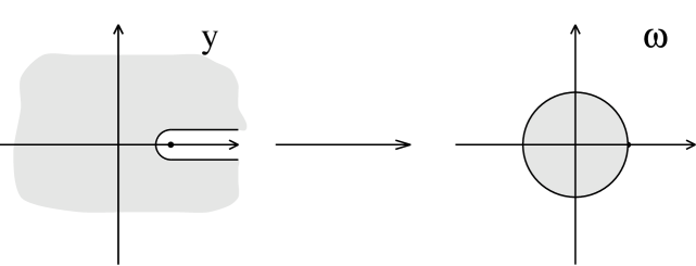
Figure 2: Conformal mapping of the $y=q^{2}/4m_{\rm t}^{2}$-complex plane into the $\omega$-plane.

By this conformal transformation, the $y$-plane, cut from $y_{0}$ to $+\infty$, is mapped into the unit circle (see Fig.2) and the cut itself is mapped on its boundary, the upper semicircle corresponding to the upper side of the cut. The origin goes into the point $\omega=0$.

After conformal transformation it is suggestive to improve the convergence of the new series w.r.t. $\omega$ by applying the Padé method [9],[10]. A convenient technique for the evaluation of Padé approximations is the $\varepsilon$-algorithm of [9] which allows one to evaluate the Padé approximants recursively.

Many interesting examples for the efficiency of this method have been worked out in the meantime and we refer to the literatur for massive diagrams to [3], [12], [13] e.g.

3 Two-loop vertex diagrams with zero thresholds

Concerning the vertex diagrams, there are many different topologies contributing to a 3-point function in the SM. For our purpose of demonstrating the method, we confine ourselves to the planar case shown in Fig. 3a. Fig. 3c,d presents infrared divergent diagrams.

Figure 3: Planar diagrams with zero thresholds. a)—generic; b)—IR finite diagram; c),d)—IR divergent diagrams.

As a typical (and very complicated case) we consider here Fig. 3b with equal non-zero masses [14]. There are two massless cuts so that we shall have the double logarithm in the expansion. After summing up four contributions we see that the double and single poles in $\varepsilon$ cancel as well as the scale parameter $\mu$, with the result $(x=q^{2}/M^{2})$

$$F(q^{2},M^{2})=\frac{1}{M^{4}}\sum_{n=0}^{\infty}\sum_{j=0}^{2}f_{jn}\ln^{j}(-x)x^{n}$$

$$\equiv\frac{1}{M^{4}}\left\{f_{0}(x)+f_{1}(x)\ln(-x)+f_{2}(x)\ln^{2}(-x)\right\},$$ (11)

where the $f_{jn}$ are now given in terms of rational numbers and $\zeta(2)$. $f_{2}(x)$ can be summed analytically, yielding

$$f_{2}(x)=\bigl{(}\ln|1+x|-i\pi\theta(1+x)\bigr{)}^{2}/x^{2}\,.$$ (12)

Thus, we have to Padé approximate $f_{0}$ and $f_{1}$ only. Close to the second threshold at $q^{2}=M^{2}$ the convergence is indeed excellent (see Table 1) [14]. It should be noted that for the physical application we have in mind, i.e. $Z\to b\bar{b}$, this is just the case of interest. It is worthwhile to note the sharp increase for low $q^{2}$ due to $\ln^{2}(-q^{2}/M^{2})$.

The infrared divergent diagrams (Fig. 3c,d) have been successfully considered in [15].

Table 1: Results for timelike $q^{2}$ for diagram 3b.

$q^{2}/M^{2}$	[12/12]		[15/15]
	Re	Im	Re	Im
00.05	$+$2.948516245	20.938528	$+$2.948516245	20.938528
00.10	$-$1.108116127	16.04132127	$-$1.108116127	16.04132127
00.50	$-$4.820692281	05.066080015	$-$4.820692281	05.066080015
01.00	$-$3.890154	01.67549787	$-$3.890156	01.67549788
01.50	$-$2.904588	00.42979	$-$2.904581	00.429778
02.00	$-$2.18294	$-$0.06976	$-$2.182981	$-$0.069728
10.00	$-$0.191	$-$0.208	$-$0.194	$-$0.215

4 The Differential Equation Method

We saw that to obtain the expansion of a diagram one has to go through a rather combersome machinery. The more coefficients are asked for, the more efforts and machine resourses are required. Thus it is very desirable to have analytic expressions for expansion coefficients whenever possible. This can be done with the aid of the Differential Equation Method (DEM) [16] if only one non-zero mass occurs. The DEM allows one to get results for massive diagrams by reducing the problem to diagrams with simpler structure.

Let us introduce a graphical notation for the scalar propagators (in euclidean space-time)

$\frac{\displaystyle 1}{\displaystyle(q^{2})^{\alpha}}\,=\;\;$ $,\qquad\frac{\displaystyle 1}{\displaystyle(q^{2}+m^{2})^{\alpha}}\,=\;\;$
$\alpha$ and $m$ refer to the index and mass of a line. Then one can derive the following recurrence relation for a massive triangle [16]

$(D-2\alpha_{1}-\alpha_{2}-\alpha_{3})\,=\,-2m_{1}^{2}\alpha_{1}\,\,\,$

          $+\alpha_{2}\Biggl{(}\;\;$ $-\;\;\;\;\;$ $\,-(m_{1}^{2}+m_{2}^{2})\;\;\;\;$ $\Biggr{)}+(\alpha_{2}\leftrightarrow\alpha_{3})$
along with some other graphical relations (see details in [16]).

Using this technique we analysed in [17] the class of 3-point two-loop massive graphs. As an example for the diagram of Fig.3c we get

$(D-4)J_{\rm 5c}\,=\,2\!\!$ $\!\!-\,2\;$ $-\,4m^{2}$ $-\,2m^{2}$ (10)

In the r.h.s. of (10) the last two terms can be combined, resulting in ${\rm d}J/{\rm d}m^{2}$ while for the second term we proceed in turn as

$(D-4)$ $=$ $+$ $-$ (11)

Thus we are left with simple diagrams (these can be done completely by Feynman parameters) and the derivative of the initial diagram w.r.t. $m^{2}$. The solution of the corresponding differential equation in terms of a series obtained from an integral representation reads

$$J_{\rm 5c} = -\frac{\Gamma^{2}(1+\varepsilon)}{{(q^{2})}^{2}{(m^{2})}^{2\varepsilon}}\sum^{\infty}_{n=1}\frac{(-x)^{n}\Gamma^{2}(n)}{\Gamma(2n+1)}\Biggl{[}\frac{1}{\varepsilon^{2}}~{}-~{}\frac{1}{\varepsilon}\biggl{(}\ln(x)+S_{1}(n-1)\biggr{)}-\frac{3}{2}S_{2}(n-1)$$

$$- \frac{15}{2}S^{2}_{1}(n-1)+4S_{1}(n-1)S_{1}(2n)-\zeta(2)-\ln(x)S_{1}(n-1)+\frac{1}{2}\ln^{2}(x)\Biggr{]},$$

where

$$S_{l}(n)=\sum^{n}_{1}\frac{1}{k^{l}}$$

A similar formula was obtained for the diagram of Fig.3d (see [17]).

5 Large mass expansion versus small momentum expansion

If there are two or more different masses involved the coefficients $a_{lmn}$ in (1) are not just numbers any more but complicated functions of mass ratios. If one of the masses is large, e.g. if the diagram contains a top, one can try to perform a large mass (LM, see [18]) expansion rather than a small momentum expansion.

Let us consider the diagram with $m_{1}=m_{2}=m_{top},m_{1}=m_{2}=m_{5}=0$ and $m_{6}=m_{W}$ (see e.g. [19]). There are again three subgraphs to be expanded. By direct evaluation we find that there are induced poles of the order $1/\epsilon^{3}$ in subgraphs while in the sum they cancel which serves as a good check. For this particular diagram the result of the LM expansion looks like

$${\rm~{}~{}~{}~{}~{}~{}~{}~{}~{}~{}~{}~{}~{}~{}~{}~{}dia} = \sum_{n=-1}^{\infty}A_{n}=\left(b^{(0)}_{n}+b^{(1)}_{n}L+b^{(2)}_{n}L^{2}+b^{(3)}_{n}L^{3}\right)\left(\frac{1}{m_{\rm top}^{2}}\right)^{n}\,~{}~{}~{}~{}~{}~{}~{}~{}~{}~{}~{}~{}~{}~{}~{}~{}~{}~{}~{}~{}~{}~{}~{}~{}~{}~{}~{}~{}~{}~{}~{}~{}~{}(12)$$

with $L=\log(m_{\rm top}^{2}/\mu^{2})$ and $b^{(i)}_{n}$’s being known functions of $q^{2},\,m_{W}^{2}$ and $\mu^{2}$.

The considered diagram is evaluated numerically at $\mu=m_{\rm top}=180\,,m_{W}=80\,,q^{2}=90^{2}$. It turns out that also here again it is extremely useful to improve the convergence of the LM expansions by applying Padé approximants. Up to a normalization factor $\frac{1}{16\pi^{2}}\frac{1}{m_{top}^{4}}$ we obtain for the diagram (-9.996,17.9527), taking into account terms up to n=10 in (12). The Taylor expansion with 8 coefficients yields a precision of appr. 10 decimals the reason for which is that $q^{2}$ is far below the threshold. The advantage of the LM expansion, however, is that it is easier to program and for many purposes the achieved precision is high enough.

6 Conclusion

Any involved calculation in field theory nessesarily consists of two parts: 1)automatic generation of Feynman diagrams and source codes and 2)techniques of evaluating scalar Feynman diagrams. In our contributions we presented both and the methods have a standard that soon important applications can be considered.

References

- [1] A.I. Davydychev and J.B. Tausk, Nucl. Phys., B397 (1993) 123.
- [2] D.J. Broadhurst, J. Fleischer and O.V. Tarasov, Z.Phys., C 60 (1993) 287.
- [3] J. Fleischer and O.V. Tarasov, Z.Phys., C 64 (1994) 413.
- [4] J. Fleischer and O.V. Tarasov, in proceedings of the ZiF conference on Computer Algebra in Science and Engineering, Bielefeld, 28-31 August 1994, World Scientific 1995, J. Fleischer, J. Grabmeier, F.W.Hehl and W.Küchlin editors.
- [5] K.G. Chetyrkin and F.V. Tkachov, Nucl. Phys. B192 (1981) 159; F.V. Tkachov, Phys. Lett. 100B (1981) 65.
- [6] D.H. Bailey, ACM Transactions on Mathematical Software, 19 (1993) 288.
- [7] A.I. Davydychev and J.B. Tausk, Nucl. Phys., B465 (1996) 507.
- [8] O.V. Tarasov, Nucl. Phys., B480 (1996) 397.
- [9] D. Shanks, J. Math. and Phys. (Cambridge, Mass.) 34 (1955) 1; P. Wynn, Math. Comp. 15 (1961) 151; G.A. Baker, P. Graves-Morris, Padé approximants, in Encyl.of math.and its appl., Vol. 13, 14, pp Addison-Wesley (1981).
- [10] G.A. Baker, Jr., J.L. Gammel and J.G. Wills, J.Math.Anal.Appl., 2 (1961) 405; G.A. Baker, Jr., Essentials of Padé Approximants, pp Academic Press (1975).
- [11] A. Djouadi, M. Spira and P.M. Zerwas, Phys. Lett., B311 (1993) 255.
- [12] J.Fleischer, Proceedings of Fourth International Workshop on Software Engineering, Artificial Intelligence and Expert System for High Energy and Nuclear Physics (Pisa, Italy, April 3-8, 1995), p 103.
- [13] J. Fleischer and O.V. Tarasov, Proceedings of the 1996 Zeuthen Workshop on Elementary Particle Theory : QCD and QED in higher Orders (Rheinsberg, Germany, April 21 - 26, 1996).
- [14] J. Fleischer, V. Smirnov and O.V. Tarasov, Z. Phys. C74 (1997) 379.
- [15] J. Fleischer et al., hep-ph/9704353, to be published in Z. Phys. C.
- [16] A.V. Kotikov, Phys.Lett. B254 (1991) 185; ibid. B259 (1991) 314; ibid. B267 (1991) 123.
- [17] J. Fleischer, A.V. Kotikov and O.L. Veretin, Bielefeld preprint BI-TP-97/26, Phys.Lett. in print; (hep-ph/9707492).
- [18] F.V. Tkachov, Preprint INR P-0332, Moscow (1983); P-0358, Moscow (1984); K.G. Chetyrkin, Teor. Math. Phys. 75 (1988), 26; ibid 76 (1988), 207; Preprint, MPI-PAE/PTh-13/91, Munich (1991); V.A. Smirnov, Comm. Math. Phys. 134 (1990), 109; Renormalization and asymptotic expansions (Birkhäuser, Basel, 1991).
- [19] J. Fleischer, M. Kalmykov and O. Veretin, Large Mass Expansion versus Small Momentum Expansion of Feynman Diagrams, Bielefeld preprint BI-TP-97/43, in preparation.