FERMILAB-Pub-98/021–A
CERN-TH/98-37
OUTP-98-02-P
hep-ph/9802238

Superheavy dark matter

Daniel J. H. Chung,^a,b, Edward W. Kolb,^b,c, Antonio Riotto^d,,
aDepartment of Physics and Enrico Fermi Institute
The University of Chicago, Chicago, Illinois 60637-1433
^bNASA/Fermilab Astrophysics Center
Fermilab National Accelerator Laboratory, Batavia, Illinois  60510-0500
^cDepartment of Astronomy and Astrophysics and Enrico Fermi Institute
The University of Chicago, Chicago, Illinois  60637-1433
^dTheory Division, CERN, CH-1211 Geneva 23, Switzerland

We show that in large-field inflationary scenarios, superheavy (many orders of magnitude larger than the weak scale) dark matter will be produced in cosmologically interesting quantities if superheavy stable particles exist in the mass spectrum. We show that these particles may be produced naturally during the transition from the inflationary phase to either a matter-dominated or radiation-dominated phase as a result of the expansion of the background spacetime acting on vacuum quantum fluctuations of the dark matter field. We find that as long as there are stable particles whose mass is of the order of the inflaton mass (presumably around $10^{13}$GeV), they will be produced in sufficient abundance to give $\Omega_{0}=1$ quite independently of any details of the non-gravitational interactions of the dark-matter field.

PACS: 98.80.Cq, 95.35.+d, 4.62.+v

I. INTRODUCTION

It is now commonly accepted that most of the mass in galactic halos as well as in the Universe as a whole is composed of dark matter (DM). There are many indications that the DM consists of some new, and yet undiscovered, weakly interacting massive particles (WIMPs).

Despite the fact that the nature of the DM is still unknown, it is usually thought that DM particles cannot be too heavy. If the WIMP is a thermal relic, then it was once in local thermodynamic equilibrium (LTE) in the early universe, and its present abundance is determined by its self-annihilation cross section. From unitarity arguments [1], one expects the mass of a thermal relic to be less than about 500 TeV. The present abundance of non-thermal relics is not determined by their self-annihilation cross section since they needn’t have been ever in LTE in the early universe. An example of a non-thermal relic is the axion, and the present axion abundance is determined by the dynamics of the phase transition associated with symmetry breaking. Non-thermal relics are typically very light, e.g., the axion mass is expected to be in the range $10^{-5}$ to $10^{-2}$eV [2].

Because the assumption of relatively low-mass DM seems quite natural, it is rarely questioned. The goal of this paper is to show that the Universe might be made of superheavy WIMPs (we will refer to them as $X$ particles), with mass larger than the weak scale by several (perhaps many) orders of magnitude. Two conditions are necessary for this to happen: a) the $X$ particles must be cosmologically stable and b) their interaction rate must be sufficiently weak such that thermal equilibrium with the primordial plasma was never obtained. This second condition is easy to satisfy as long as the particle is extremely massive (of the order of the Hubble parameter at the end of inflation).

We point out that superheavy dark matter may be created during the evolution of the Universe in a number of ways. If it is produced during the process of reheating after inflation, then the upper bound on its mass $M_{X}$ can be as large as the reheating temperature $T_{RH}$. The latter should be less than about $10^{9}$GeV in order to avoid overproducing dangerous relics such as quasistable gravitinos in supergravity inspired scenarios. The mass upper bound can be pushed higher than the reheating temperature if one allows the DM to be produced directly through the decay of the inflaton field. In that case, the mass upper bound is the inflaton field mass, which is presumably less than about $10^{13}$GeV. On the other hand, if reheating after inflation is preceded by a preheating stage [6] it is certainly possible to produce by resonance effects copious amounts of dark matter particles with masses much larger than the inflaton mass [7].

In this paper, we consider yet another mechanism of generating heavy DM. We study the possibility that DM is produced in the transition between an inflationary and a matter-dominated (or radiation-dominated) universe due to the “nonadiabatic” expansion of the background spacetime during the transition acting on the vacuum quantum fluctuations.

The distinguishing feature of this mechanism is the capability of generating particles with mass of the order of the inflaton mass (usually much larger than the reheating temperature) even when the particles only interact extremely weakly (or not at all) with other particles and do not couple to the inflaton(s). We find that they may still be produced in sufficient abundance to achieve critical density today due to the classical gravitational effect on the vacuum state at the end of inflation. More specifically, we will show that in the range $0.04\mathrel{\mathchoice{\lower 3.6pt\vbox{\halign{$\mathsurround=0pt\displaystyle\hfill#\hfil$\cr<\crcr\sim\crcr}}}{\lower 3.6pt\vbox{\halign{$\mathsurround=0pt\textstyle\hfill#\hfil$\cr<\crcr\sim\crcr}}}{\lower 3.6pt\vbox{\halign{$\mathsurround=0pt\scriptstyle\hfill#\hfil$\cr<\crcr\sim\crcr}}}{\lower 3.6pt\vbox{\halign{$\mathsurround=0pt\scriptscriptstyle\hfill#\hfil$\cr<\crcr\sim\crcr}}}}M_{X}/H\mathrel{\mathchoice{\lower 3.6pt\vbox{\halign{$\mathsurround=0pt\displaystyle\hfill#\hfil$\cr<\crcr\sim\crcr}}}{\lower 3.6pt\vbox{\halign{$\mathsurround=0pt\textstyle\hfill#\hfil$\cr<\crcr\sim\crcr}}}{\lower 3.6pt\vbox{\halign{$\mathsurround=0pt\scriptstyle\hfill#\hfil$\cr<\crcr\sim\crcr}}}{\lower 3.6pt\vbox{\halign{$\mathsurround=0pt\scriptscriptstyle\hfill#\hfil$\cr<\crcr\sim\crcr}}}}2$, where $H\sim m_{\phi}\sim 10^{13}$GeV is the Hubble constant at the end of inflation ($m_{\phi}$ being the mass of the inflaton), the DM produced gravitationally can have a density today of the order of the critical density. This result is quite robust with respect to the “fine” details of the transition between the inflationary phase and the matter-dominated phase, and independent of the coupling of the DM to any other particle. This result is reasonably robust also with respect to the ambiguity associated with the choice of the vacua as we have tried to minimize the number of particles produced by choosing an infinite adiabatic order in-out vacua. The only “non-trivial” requirements, other than that large field inflation occurs, are that the WIMPs posses a mass close to the inflaton mass and that they are stable.

Mechanically, the DM particle creation scenario is similar to the inflationary generation of gravitational perturbations that seed the formation of large scale structures (see for example the review given in Ref. [8]). In the usual scenarios of this form, however, the quantum generation of energy density fluctuations from inflation is associated with the inflaton field which dominated the mass density of the universe, and not a generic, sub-dominant scalar field.

Because it is usually assumed that DM forms from the decays or interactions of the reheating products, it usually has a stage of LTE in its early history. In our scenario the large mass of the dark-matter particle will prevent it from thermalizing, and its abundance will depend only on its mass and the behavior of the spacetime, not on its weak coupling to other nongravitational fields.

Others have considered gravitational particle production at the end of inflation. For example, Ford [9] and Yajnik [10] both consider particle production as a result of the nonadiabaticity of the transition from an inflationary phase to a matter or radiation dominated phase (although with a different cosmological implication in mind). Ford treats only massless, non-conformally coupled fields using a well known perturbation technique (see references within [9]). Yajnik considers minimally coupled scalar field theory in the limit of small masses, with an abrupt transition from an inflationary phase to a radiation dominated phase. In our work, we consider extremely massive, conformally coupled fields and calculate the particle production exactly by numerically solving the mode equation. We treat the conformally coupled case because conformal coupling generally minimizes the number of particles produced, particularly in the small mass ranges. Unlike Yajnik, we also consider the case where the metric is an analytic function of the conformal time and show that this leads to qualitatively different behavior of the density of particles produced for large masses. The analyticity implies a conservative estimate since fewer particles are produced in that case than in the abrupt transition case.

Some of the ideas present in our scenario are also contained in the work of Linde and Kofman [11], [12], and [13]. However, the purpose of their work was to point out that isocurvature cosmological (large scale) perturbations can be produced during inflation. They did not consider the importance of the nonadiabaticity of the transition at the end of inflation which is responsible for the production of our superheavy dark matter. Instead, they mainly relied upon estimates of the particle production during the de Sitter phase or the classical (long wavelength) component of the particle field energy density left over after inflation.

This paper is organized as follows. In the next section, we elaborate on the dark matter scenario and the calculational method. In Section III, we discuss the numerical results. We then summarize our work in Section IV. In the appendix, we derive the asymptotic mass dependence of the dark matter density presented in Section II.

II. SCENARIO AND CALCULATIONAL METHOD

In this section we discuss the dark matter abundance calculation in our scenario. First, we give an expression for the dark matter density today in terms of the number density when it was produced. We then consider the mass range of the dark matter necessary if it is never to thermalize. Finally, we discuss the mechanics of the gravitational production of particles. In particular, we discuss the number density definition and present the asymptotic dependence of the number density on the particle mass.

Suppose the dark matter never attains LTE and is nonrelativistic at the time of production. The usual quantity $\Omega_{X}h^{2}$ associated with the dark matter density today can be related to the dark matter density when it was produced. To develop the relation, we begin by writing

$$\frac{\rho_{X}(t_{0})}{\rho_{R}(t_{0})}=\frac{\rho_{X}(t_{RH})}{\rho_{R}(t_{RH})}\>\left(\frac{T_{RH}}{T_{0}}\right),$$ (1)

where $\rho_{R}$ denotes the energy density stored in radiation, $\rho_{X}$ denotes the energy density residing in the dark matter, $T_{RH}$ is the reheating temperature, $T_{0}$ is the temperature today, $t_{0}$ denotes the time today, and $t_{RH}$ denotes the approximate time of reheating completion. To obtain $\rho_{X}(t_{RH})/\rho_{R}(t_{RH})$, we must determine when $X$ particles are produced with respect to the completion of reheating and the effective equation of state operative between $X$ production and the completion of reheating.

At the end of inflation the universe may have a brief period of matter domination resulting either from the coherent oscillations phase of the inflaton condensate or from the preheating phase [6]. If the $X$ particles are produced at time $t=t_{e}$ when the de Sitter phase ends and the coherent oscillation period just begins, then both the $X$ particle energy density and the inflaton energy density will redshift at approximately the same rate until reheating is completed and radiation domination begins. Hence, the ratio of energy densities preserved in this way until the time of radiation domination is

$$\frac{\rho_{X}(t_{RH})}{\rho_{R}(t_{RH})}\approx\frac{8\pi}{3}\>\frac{\rho_{X}(t_{e})}{{{M_{{\rm Pl}}}}^{2}H^{2}(t_{e})},$$ (2)

where ${{M_{{\rm Pl}}}}\approx 10^{19}$ GeV is the Planck mass and most of the energy density in the universe just before time $t_{RH}$ is presumed to turn into radiation. Thus, using Eq. (1), we may get an expression for the quantity $\Omega_{X}\equiv\rho_{X}(t_{0})/\rho_{C}(t_{0})$, where $\rho_{C}(t_{0})=3H_{0}^{2}{{M_{{\rm Pl}}}}^{2}/8\pi$ and $H_{0}=100\>h$ km sec^-1 Mpc^-1:

$$\Omega_{X}h^{2}\approx\Omega_{R}h^{2}\>\left(\frac{T_{RH}}{T_{0}}\right)\>\frac{8\pi}{3}\left(\frac{M_{X}}{{{M_{{\rm Pl}}}}}\right)\>\frac{n_{X}(t_{e})}{{{M_{{\rm Pl}}}}H^{2}(t_{e})}.$$ (3)

Here $\Omega_{R}h^{2}\approx 4.31\times 10^{-5}$ is the fraction of critical energy density that is in radiation today and $n_{X}$ is the density of $X$ particles at the time when they were produced.

Note that because the reheating temperature must be much greater than the temperature today ($T_{RH}/T_{0}\mathrel{\mathchoice{\lower 3.6pt\vbox{\halign{$\mathsurround=0pt\displaystyle\hfill#\hfil$\cr>\crcr\sim\crcr}}}{\lower 3.6pt\vbox{\halign{$\mathsurround=0pt\textstyle\hfill#\hfil$\cr>\crcr\sim\crcr}}}{\lower 3.6pt\vbox{\halign{$\mathsurround=0pt\scriptstyle\hfill#\hfil$\cr>\crcr\sim\crcr}}}{\lower 3.6pt\vbox{\halign{$\mathsurround=0pt\scriptscriptstyle\hfill#\hfil$\cr>\crcr\sim\crcr}}}}4.2\times 10^{14}$), in order to satisfy the cosmological bound $\Omega_{X}h^{2}\mathrel{\mathchoice{\lower 3.6pt\vbox{\halign{$\mathsurround=0pt\displaystyle\hfill#\hfil$\cr<\crcr\sim\crcr}}}{\lower 3.6pt\vbox{\halign{$\mathsurround=0pt\textstyle\hfill#\hfil$\cr<\crcr\sim\crcr}}}{\lower 3.6pt\vbox{\halign{$\mathsurround=0pt\scriptstyle\hfill#\hfil$\cr<\crcr\sim\crcr}}}{\lower 3.6pt\vbox{\halign{$\mathsurround=0pt\scriptscriptstyle\hfill#\hfil$\cr<\crcr\sim\crcr}}}}1$, the fraction of total energy density in the dark matter at the time when they were produced must be extremely small. To illustrate this, take $H^{2}(t_{e})\sim m_{\phi}^{2}$ and $\rho(t_{e})\sim m_{\phi}^{2}{{M_{{\rm Pl}}}}^{2}$. Then $\Omega_{X}h^{2}\sim 10^{17}(T_{RH}/10^{9}\mbox{GeV})(\rho_{X}(t_{e})/\rho(t_{e}))$. It is indeed a very small fraction of the total energy density we wish to extract in the form of massive $X$ particles.

This means that if the dark matter particle is extremely massive, the challenge lies in creating very few of them naturally. We will see that the gravitational production naturally gives the needed suppression. Note that if reheating occurs abruptly at the end of inflation, then the matter domination phase may be negligibly short and the radiation domination phase may follow immediately after the end of inflation. However, this does not change Eq. (3).

For the superheavy $X$ particles to be good candidates for DM, they have to be stable or at least have a lifetime greater than the age of the universe. This may occur in supersymmetric theories where the breaking of supersymmetry is communicated to the ordinary sparticles via the usual gauge forces [14]. In gauge-mediated supersymmetric models there are two sectors with possible stable particles which might act as superheavy dark matter candidates:

1) The secluded sector, which is strongly interacting: Supersymmetry is broken dynamically and some $F$-term gets a nonvanishing expectation value, where the scale of supersymmetry breaking, as usual, is denoted by $\sqrt{F}$.

2) The messenger sector: This sector contains the fields charged under the $SU(3)_{C}\otimes SU(2)_{L}\otimes U(1)_{Y}$ gauge interactions, and communicate supersymmetry breaking to the sparticles in the observable sector. The mass of the messenger fields is usually denoted by $M$.

After the messengers have been integrated out, sfermions receive a mass squared $\widetilde{m}^{2}\sim\alpha^{2}\Lambda^{2}$, where $\alpha$ is the appropriate gauge coupling and $\Lambda\simeq F/M$. Notice, in particular, that the spectrum of the superparticles depends on the ratio $\Lambda=F/M$ which is fixed to be relatively small and in the range $10$ to $10^{3}$ TeV. However, this does not necessarily mean that $\sqrt{F}$ and $M$ are of the same order of magnitude as $\Lambda$ [15] since it is only their ratio which is fixed around $10^{3}$ TeV: the hierarchy $\sqrt{F},M\gg\Lambda$ is certainly allowed [16].

The secluded sector often has accidental symmetries analogous to the baryon number. This means that the lightest particle in the secluded sector might be stable and a good candidate for dark matter with a mass of the order of $\sqrt{F}$, much larger than the weak scale. The lightest messenger field might also be a good candidate for superheavy DM. Indeed, if the supersymmetry breaking sector contains only singlets under the $SU(3)_{C}\otimes SU(2)_{L}\otimes U(1)_{Y}$ gauge interactions and if there are no direct couplings between the ordinary and messenger sectors, then the theory is characterized by a conserved global quantum number carried only by the messenger fields. The typical mass $M$ of the DM component in the messenger sector may be much larger than the weak scale.

Another framework in which we might expect the presence of superheavy stable particles is a Kaluza-Klein theory (a unified theory which requires space-time dimensions higher than four). A popular example is provided by M-theory [17] where the number of dimensions is $D=11$. These theories are characterized by the presence of a tower of Kaluza-Klein modes which are left after the compactification of the extra $D-4$ dimensions. For instance, if $D=5$, the existence of a compact fifth dimension implies an infinite tower of four-dimensional particles corresponding to quantized excitations of the extra dimension. These massive particles have been called “pyrgons” [18]. If any of the pyrgon states are stable or have a lifetime greater than the age of the universe, they might act as DM with a mass of the order of the inverse of the physical size of the compact dimensions $R_{D}^{-1}$, which is likely to be larger than the weak scale by many orders of magnitude.

For the gravitational production scenario to be distinguishable from other scenarios, $X$ must never thermalize. The condition for the dark matter particles to be out of equilibrium and their comoving number density to be constant is

$$n_{X}\langle\sigma_{A}|v|\rangle\mathrel{\mathchoice{\lower 3.6pt\vbox{\halign{$\mathsurround=0pt\displaystyle\hfill#\hfil$\cr<\crcr\sim\crcr}}}{\lower 3.6pt\vbox{\halign{$\mathsurround=0pt\textstyle\hfill#\hfil$\cr<\crcr\sim\crcr}}}{\lower 3.6pt\vbox{\halign{$\mathsurround=0pt\scriptstyle\hfill#\hfil$\cr<\crcr\sim\crcr}}}{\lower 3.6pt\vbox{\halign{$\mathsurround=0pt\scriptscriptstyle\hfill#\hfil$\cr<\crcr\sim\crcr}}}}H,$$ (4)

where $H$ is the Hubble parameter, $\langle\sigma_{A}|v|\rangle$ is the thermal averaged self-annihilation cross section times the Møller speed for the dark matter particles $X$. Since the cross section $\sigma_{A}$ is expected to be at most about $M_{X}^{-2}$ (usually smaller; sometimes much smaller) and $n_{X}$ is bounded by the condition that $\Omega_{X}h^{2}<1$, we obtain from Eq. (3)

$$\frac{n_{X}\langle\sigma_{A}|v|\rangle}{H}\approx\frac{7\times 10^{-19}}{(T_{RH}/10^{9}\mbox{GeV})}\ \frac{(H/{{M_{{\rm Pl}}}})}{(M_{X}/{{M_{{\rm Pl}}}})^{3}}$$ (5)

as the quantity which must be less than one at $t=t_{e}$ to avoid thermalization. For a low reheating temperature of $10^{2}$ GeV and a typical value of $H=10^{-6}{{M_{{\rm Pl}}}}$ for inflationary scenarios, we find a conservative condition $M_{X}/H\mathrel{\mathchoice{\lower 3.6pt\vbox{\halign{$\mathsurround=0pt\displaystyle\hfill#\hfil$\cr>\crcr\sim\crcr}}}{\lower 3.6pt\vbox{\halign{$\mathsurround=0pt\textstyle\hfill#\hfil$\cr>\crcr\sim\crcr}}}{\lower 3.6pt\vbox{\halign{$\mathsurround=0pt\scriptstyle\hfill#\hfil$\cr>\crcr\sim\crcr}}}{\lower 3.6pt\vbox{\halign{$\mathsurround=0pt\scriptscriptstyle\hfill#\hfil$\cr>\crcr\sim\crcr}}}}1$ for the particles never to reach chemical thermal equilibrium. Note that this is a rather conservative estimate since the reheating temperature is likely to be larger and the cross section is likely to be smaller. We also remark that because the reheating temperature is likely to be much smaller than the $X$ mass, the thermal production of the $X$ particles is negligible.

Now let us describe the basic physics underlying our mechanism of gravitational production of DM.

In this paper we take space-time both in and out of inflationary era to be spatially flat, homogeneous, and isotropic, with the line element of the form

$$ds^{2}=a^{2}(\eta)(d\eta^{2}-d{\bf x}^{2}).$$ (6)

For simplicity (and without much loss of generality), we restrict ourselves to a massive scalar field coupled to classical gravity and nothing else. The other couplings are assumed to play an insignificant role in the gravitational production.

There are various inequivalent ways of calculating the particle production due to interaction of a classical gravitational field with the vacuum (see for example [19], [20], and [21]). In our work, we use the method of finding the Bogoliubov coefficient for the transformation between positive frequency modes defined at two different times. We will show below that the large mass dependence of the DM number density is determined by either the differentiability (or the smoothness) of the scale factor or the choice of the vacuum. On the other hand, for $M_{X}/H\mathrel{\mathchoice{\lower 3.6pt\vbox{\halign{$\mathsurround=0pt\displaystyle\hfill#\hfil$\cr<\crcr\sim\crcr}}}{\lower 3.6pt\vbox{\halign{$\mathsurround=0pt\textstyle\hfill#\hfil$\cr<\crcr\sim\crcr}}}{\lower 3.6pt\vbox{\halign{$\mathsurround=0pt\scriptstyle\hfill#\hfil$\cr<\crcr\sim\crcr}}}{\lower 3.6pt\vbox{\halign{$\mathsurround=0pt\scriptscriptstyle\hfill#\hfil$\cr<\crcr\sim\crcr}}}}1$ where $H$ is the value at the end of inflation, the results are quite insensitive to the differentiability or the fine details of the scale factor’s time dependence. For $0.04\mathrel{\mathchoice{\lower 3.6pt\vbox{\halign{$\mathsurround=0pt\displaystyle\hfill#\hfil$\cr<\crcr\sim\crcr}}}{\lower 3.6pt\vbox{\halign{$\mathsurround=0pt\textstyle\hfill#\hfil$\cr<\crcr\sim\crcr}}}{\lower 3.6pt\vbox{\halign{$\mathsurround=0pt\scriptstyle\hfill#\hfil$\cr<\crcr\sim\crcr}}}{\lower 3.6pt\vbox{\halign{$\mathsurround=0pt\scriptscriptstyle\hfill#\hfil$\cr<\crcr\sim\crcr}}}}M_{X}/H\mathrel{\mathchoice{\lower 3.6pt\vbox{\halign{$\mathsurround=0pt\displaystyle\hfill#\hfil$\cr<\crcr\sim\crcr}}}{\lower 3.6pt\vbox{\halign{$\mathsurround=0pt\textstyle\hfill#\hfil$\cr<\crcr\sim\crcr}}}{\lower 3.6pt\vbox{\halign{$\mathsurround=0pt\scriptstyle\hfill#\hfil$\cr<\crcr\sim\crcr}}}{\lower 3.6pt\vbox{\halign{$\mathsurround=0pt\scriptscriptstyle\hfill#\hfil$\cr<\crcr\sim\crcr}}}}2$, we find that all the dark matter needed for closure of the universe can be made gravitationally, quite independently of the details of the transition between the inflationary phase and the matter dominated phase.

To see the effects of vacuum choice and the scale factor differentiability on the large $X$ mass behavior of the $X$ density produced, we start with the canonical quantization of the $X$ field in an action of the form (in the coordinate $ds^{2}=dt^{2}-a^{2}(t)d\bf{x}^{2}$)

$$S=\int dt\int d^{3}\!x\,\frac{a^{3}}{2}\left(\dot{X}^{2}-\frac{(\nabla X)^{2}}{a^{2}}-M_{X}^{2}X^{2}-\xi RX^{2}\right)$$ (7)

where $R$ is the Ricci scalar. After transforming to conformal time coordinate, we use the mode expansion

$$X({\bf x})=\int\frac{d^{3}\!k}{(2\pi)^{3/2}a(\eta)}\left[a_{k}h_{k}(\eta)e^{i{\bf{k\cdot x}}}+a_{k}^{\dagger}h_{k}^{*}(\eta)e^{-i{\bf{k\cdot x}}}\right],$$ (8)

where because the creation and annihilation operators obey the commutator $[a_{k_{1}},a_{k_{2}}^{\dagger}]=\delta^{(3)}({\bf k}_{1}-{\bf k}_{2})$, the $h_{k}$s obey a normalization condition $h_{k}h_{k}^{{}^{\prime}*}-h_{k}^{\prime}h_{k}^{*}=i$ to satisfy the canonical field commutators (henceforth, all primes on functions of $\eta$ refer to derivatives with respect to $\eta$). The resulting mode equation is

$$h_{k}^{\prime\prime}(\eta)+w_{k}^{2}(\eta)h_{k}(\eta)=0,$$ (9)

where

$$w_{k}^{2}=k^{2}+M_{X}^{2}a^{2}+(6\xi-1)a^{\prime\prime}/a\ .$$ (10)

The parameter $\xi$ is 1/6 for conformal coupling and 0 for minimal coupling. From now on, we will set $\xi=1/6$ for simplicity but without much loss of generality. By a change in variable $\eta\rightarrow k/a$, one can rewrite the differential equation such that it depends only on $H(\eta)$, $H^{\prime}(\eta)/k$, $k/a(\eta)$, and $M_{X}$. Hence, we introduce the parameter $H_{i}$ and $a_{i}$ corresponding to the Hubble parameter and the scale factor evaluated at an arbitrary conformal time $\eta_{i}$, which we take to be the approximate time at which $X$ are produced (i.e., $\eta_{i}=\eta(t_{e})$). We then rewrite Eq. (9) as

$$h_{{\tilde{k}}}^{\prime\prime}({{\tilde{\eta}}})+({{\tilde{k}}}^{2}+b^{2}\tilde{a}^{2})h_{{\tilde{k}}}({{\tilde{\eta}}})=0\qquad[b\equiv M_{X}/H_{i}]$$ (11)

where ${{\tilde{\eta}}}=\eta a_{i}H_{i}$, $\tilde{a}=a/a_{i}$, and ${{\tilde{k}}}=k/(a_{i}H_{i})$. For simplicity of notation, we shall drop all the tildes from now on. This differential equation can be solved once the boundary conditions are supplied. Since the annihilation operator is just a coefficient of an expansion in a particular basis, fixing the boundary conditions is equivalent to fixing the vacuum.

To obtain the number density of the particles produced, we will perform a Bogoliubov transformation from the vacuum mode solution with the boundary condition at $\eta=\eta_{0}$ (the initial time at which the vacuum of the universe is determined) into the one with the boundary condition at $\eta=\eta_{1}$ (any later time at which the particles are no longer being created). In the examples given in the next section, $\eta_{0}$ will be taken to be $-\infty$ while $\eta_{1}$ will be taken to be at $+\infty$ in order to define vacua of infinite adiabatic order (explained below) which results in a smaller particle production than for any finite adiabatic order vacua. The exact values of $\eta_{0}$ and $\eta_{1}$ are not important for those examples as long as they are in a region in which $a^{\prime}/a^{2}\ll 1$ or $ba/k\ll 1$. Defining the Bogoliubov transformation as $h_{k}^{\eta_{1}}(\eta)=\alpha_{k}h_{k}^{\eta_{0}}(\eta)+\beta_{k}h_{k}^{*\eta_{0}}(\eta)$ (the superscripts denote where the boundary condition is set), we have the following energy density in the particles produced:

$$\rho_{X}(\eta_{1})=M_{X}n_{X}(\eta_{1})=M_{X}H_{i}^{3}\left(\frac{1}{\tilde{a}(\eta_{1})}\right)^{3}\int_{0}^{\infty}\frac{d\tilde{k}}{2\pi^{2}}\tilde{k}^{2}|\beta_{\tilde{k}}|^{2},$$ (12)

where one should note that the number operator is defined at $\eta_{1}$ while the quantum state (approximated to be the vacuum state) defined at $\eta_{0}$ does not change in time in the Heisenberg representation.

As usual, there is an ambiguity in the definition of the vacuum, which is equivalent to an ambiguity in the boundary conditions of Eq. (9). One method of systematically classifying the various inequivalent vacuum states is through the adiabatic vacuum [22] definition. The adiabatic vacuum definition allows one to construct and classify a set of mode equation solutions which reduce to the usual plane waves when $a^{\prime}(\eta)=0$ for all $\eta$. The classification is based on a type of WKB asymptotic expansion in powers of conformal time derivatives of $w_{k}$. In particular, the classification allows one to quantify how two solutions with different boundary conditions (hence two vacua) will differ in terms of derivatives of $w_{k}$. Each derivative with respect to the conformal time is assigned a bookkeeping small parameter, and this small parameter’s power in an expansion is referred to as the adiabatic order. We define $A$th adiabatic (order) vacuum at time $\eta^{*}$ by using the boundary condition

$$h_{k}(\eta^{*})=h_{k}^{(A)}(\eta^{*}),\qquad h_{k}^{\prime}(\eta^{*})=h_{k}^{{}^{\prime}(A)}(\eta^{*}),$$ (13)

where $h_{k}^{(A)}(\eta)$ is a systematically chosen approximate solution to the mode equation that satisfies the mode equation up to $A$th adiabatic order in the asymptotic limit that the adiabatic parameter goes to zero. Roughly speaking, the larger the adiabatic order of the vacuum, the closer it is to the Minkowski vacuum in the sense that it is less (in the adiabatic limit) dependent on the time at which it is defined. We refer the reader to the appendix (or Ref. [20]) for a more precise definition.

As shown in the appendix, the asymptotic behavior of the number density as $b\rightarrow\infty$ can be obtained by the following rule: If the vacuum at $\eta_{0}$ corresponds to an $n$th adiabatic vacuum, and the vacuum at $\eta_{1}$ corresponds to a $p$th adiabatic vacuum, then as $b\rightarrow\infty$ the number density will behave like

$$n_{X}\sim b^{-(2r+1)}$$ (14)

where $r=\mbox{Min}(p,n)$ provided that $(d^{\nu}a/d\eta^{\nu})/a^{\nu+1}<\infty$ for all $\eta\in[\eta_{0},\eta_{1}]$ and all natural numbers $\nu$. It is important to note that for a fixed time, the asymptotic expansion generated by Eq. (A2) (in the Appendix) generally only converges up to a finite order. Hence, except under special circumstances an adiabatic vacuum of only a finite order can be generated. This means that in general, the number density will fall off with a finite power of $1/b$ for large $b$. Only when an adiabatic vacuum of infinite adiabatic order can be generated, which usually means that the domain of $a(\eta)$ can be extended to $\pm\infty$ with the property given above, does the number of particles produced fall off faster than any finite power of $1/b$ (e.g., exponential suppression). In practice, we find that a spacetime which admits an infinite adiabatic order vacuum has the “advantage” of all the vacua defined in a sufficiently adiabatic region being numerically equivalent regardless of the vacua’s adiabatic order and the exact time at which the vacua are defined.

If within the domain there is one discontinuity of the first kind in $(d^{q}a/d\eta^{q})/a^{q+1}$ for $q=s$ where $-2<s-2\leq r=\mbox{Min}(p,n)$ and there are no discontinuities for $q<s$,

$$n_{X}\sim b^{-(2s-3)}.$$ (15)

This is true provided that $(d^{\nu}a/d\eta^{\nu})/a^{\nu+1}<\infty$ for all $\eta$ in each of the continuous domain and all natural numbers $\nu$. Note that fractional power dependence on $1/b$ will be possible if the discontinuity is not of the first kind (e.g., $a(\eta)=\eta^{2}$ at $\eta=0$).

III. NUMERICAL RESULTS

We shall employ the method elaborated in the previous section to calculate the gravitational production of particles in a couple of toy models of inflation which reflect some extreme ranges of differentiability. We will consider the case when the scale factor has a discontinuity of the first kind in one of its derivatives and when it is a $C^{\infty}$ function. We will see that enough dark matter may be produced through this mechanism as to give critical density of dark matter today.

Our example of a discontinuous model has the scale factor of the de Sitter space for $\eta<\eta_{i}$ and the matter or radiation dominated universe for $\eta>\eta_{i}$:

$$a(\eta)=\left\{\begin{array}[]{ll}a_{i}/(2-\eta/\eta_{i})&\qquad\mbox{if $\eta\leq\eta_{i}$},\\ a_{i}(\eta/\eta_{i})^{p}&\qquad\mbox{if $\eta>\eta_{i}$},\end{array}\right.$$ (16)

where $p=2$ for the matter dominated case and $p=1$ for the radiation dominated case. If we define our vacuum states at $\eta_{0}=-\infty$ and $\eta_{1}=\infty$, then in this space time, adiabatic vacua of any order will be equivalent to infinite-order adiabatic vacua. For the transition into matter domination, the smallest derivative order in which there is a discontinuity (of the first kind) comes from $a^{\prime}(\eta)$ at $\eta=\eta_{i}$ while for the transition into the radiation domination, the analogous contribution comes from $a^{\prime\prime}(\eta)$ which has a discontinuity of the first kind at $\eta=\eta_{i}$. Hence, our analysis would predict that for large $b$, $n_{X}$ will increase like $b$ in the case of matter domination whereas it will fall off like $1/b$ in the case of radiation domination.

Figure 1: The scale factor (normalized to its value at $\eta=\eta_{i}$) is plotted as a function of the scaled conformal time $\eta/\eta_{i}$. The curves labeled “smooth” and “discontinuous” correspond to the toy models for the evolution of the scale factor without and with discontinuous derivatives, respectively. As $\eta/\eta_{i}\rightarrow-\infty$, the scale factor behaves as $1/(\eta/\eta_{i})^{2}$ corresponding to a de Sitter space, and as $\eta/\eta_{i}\rightarrow+\infty$, the scale factor behaves as $(\eta/\eta_{i})^{2}$ corresponding to a matter dominated Universe. The solid curve shows an analogous numerical solution of the scale factor for a $(1/2)m_{\phi}^{2}\phi^{2}$ inflaton potential.

Our second toy model looks at the other extreme limit of having a $C^{\infty}$ function for $a(\eta)$ which behaves in the asymptotic limits of $\eta/\eta_{i}\rightarrow\pm\infty$ identically as the discontinuous model:

$$a(\eta) = a_{i}\left\{\frac{1-\exp[-(\eta/\eta_{i})^{2}]}{(\eta/\eta_{i})^{2}}\left(\frac{1-\tanh(\eta/\eta_{i}/2+1)}{2}\right)+\frac{(\eta/\eta_{i})^{2p}}{(1+3\exp(-\eta/\eta_{i}))^{2}}\right.$$ (17)

$$\left.\phantom{\frac{A}{B}}+\tanh(\eta/\eta_{i}-\lambda)-\tanh(\eta/\eta_{i}-2\lambda)\right\}^{1/2}$$

where $\lambda=1.07$ is needed for proper normalization. The functional form was chosen rather arbitrarily except for the requirements of monotonicity, $(d^{\nu}a/d\eta^{\nu})/a^{\nu+1}<\infty$ for all $\eta$ and natural numbers $\nu$, and appropriate power law asymptotic behavior. As before, this spacetime admits a vacuum of infinite adiabatic order at $\eta=\pm\infty$. In Fig. 1 we show how these models compare with the numerical result obtained by solving the $(1/2)m_{\phi}^{2}\phi^{2}$ inflationary model’s equations of motion. Note that they differ mainly in the transition region (or the “nonadiabatic” region near $\eta/\eta_{i}=1$) where most of the particle production “occurs.”

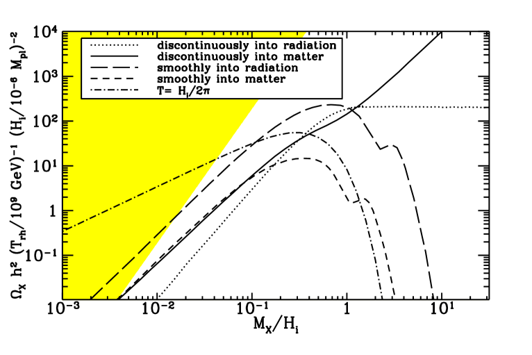
Figure 2: The dark matter abundance today is shown as a function of the particle mass for various models. The mass is given in terms of $H_{i}\approx 10^{-6}{{M_{{\rm Pl}}}}$ (the Hubble parameter at $\eta=\eta_{i}$, the beginning of the coherent oscillation period). In the “discontinuously into radiation” case, $a^{\prime\prime}(\eta)$ has a discontinuity at $\eta=\eta_{i}$, while in the “discontinuously into matter” case, $a^{\prime}(\eta)$ has a discontinuity at $\eta=\eta_{i}$. The curves labeled “smoothly into” is for $a(\eta)$ that satisfies $(d^{\nu}a/d\eta^{\nu})/a^{\nu+1}<\infty$ for all $\eta$ and natural numbers $\nu$. The curve labeled $T=H_{i}/(2\pi)$ shows a thermal density with this temperature. The unshaded region satisfies the conservative nonthermalization condition obtained by setting $\langle\sigma_{A}{|}v{|}\rangle=1/M_{X}^{2}$ in Eq. (4).

In Fig. 2, we show the number density obtained numerically in these toy models. The peak at $M_{X}/H_{i}\sim 1$ for the $C^{\infty}$ model is similar to the case presented in Ref. [23]. As we expect, the large $b$ behavior is exactly determined by the choice of the vacuum and the differentiability of the potential. Specifically, just as our asymptotic analysis showed, for large $b$, $n_{X}$ varies as $b$ and $1/b$ for the matter and radiation domination case respectively in the discontinuous model, while $n_{X}$ is exponentially suppressed in the $C^{\infty}$ model. Note that independently of the differentiability of the scale factor, if $M_{X}\approx H_{i}\approx m_{\phi}$ for $T_{RH}\approx 10^{9}$ GeV, $X$ will have critical energy density today. On the other hand, unless there is some discontinuity in the scale factor for some $n$th derivative where $n$ is not too large, this gravitational production mechanism will not generate enough dark matter in the Universe to give critical density for much larger masses ($M_{X}\gg m_{\phi}$) even if such stable heavy particles exist. Furthermore, even in the mass range in which the density of particles produced peaks, if the reheating temperature is below about $10^{7}$ GeV, this mechanism will most likely not generate significant amount of dark matter. In the case that this mechanism cannot produces these heavy particles, however, if these heavy particles couple to the inflaton and if preheating occurs, enough of them may be produced through the broad resonance mechanism to have critical density of superheavy dark matter today.

IV. SUMMARY

To conclude, we have investigated the scenario of creating nonthermalizing dark matter gravitationally at the end of inflation (or the beginning of the coherent oscillation phase). There is a significant mass range ( $0.1m_{\phi}$ to $m_{\phi}$, where $m_{\phi}\approx 10^{13}$GeV) for which the $X$ particles will have critical density today regardless of the fine details of the inflation-matter/radiation transition. Because this production mechanism is inherent in the dynamics between the classical gravitational field and a quantum field, it needs no fine tuning of field couplings or any coupling to the inflaton field. However, only if the particles are stable (or sufficiently long lived) will these particles give contribution of the order of critical density. For even larger dark matter masses, the broad resonance mechanism of preheating (if it occurs) will produce these particles in sufficient abundance as to achieve $\Omega_{0}=1$.

ACKNOWLEDGMENTS

We would like to thank Robert Wald, Ewan Stewart, Andrei Linde, Lev Kofman, Norbert Schörghofer, Alvaro de Rujula, and Christoph Schmid for discussions. We would like to also thank the referee for some helpful suggestions. DJHC and EWK were supported by the DOE and NASA under Grant NAG5-2788.

APPENDIX

In this appendix, we derive Eq. (14) and Eq. (15), the asymptotic dependence of the dark matter density on the mass parameter $b=M_{X}/H_{i}$ as $b\rightarrow\infty$. This asymptotic behavior is, in general, dependent upon the choice of the vacuum state and the differentiability of the scale factor in an FRW type spacetime. We employ the adiabatic vacua ansatz [22] to classify the various possible (restricted) choices of vacua. Strictly speaking, our conditions for the various asymptotic behaviors are only sufficient conditions, but they have wide applicability as we demonstrate in this paper.

Let us first review the concept of an adiabatic vacuum (see for example pg. 66 of Ref. [20]). We first define the concept of an adiabatic order as the power of $1/T$ that results for any term in a $1/T$ expansion after one makes the transformation $\eta\rightarrow\eta$ and $d/d\eta\rightarrow T^{-1}d/d\eta$. Note that if $T^{-1}\rightarrow 0$, then this is equivalent to an expansion in “smallness” of conformal time derivatives. The basic idea is that if the derivatives of the mode frequency $w_{k}$ are indeed small, then the degree to which the field theory breaks time translational symmetry can be characterized by the adiabatic order. This breaking of the time translational symmetry is what is responsible for particle creation in our isotropic expanding Universe.

To define the adiabatic vacuum, we first make a change in variables from $h_{k}$ to $W_{k}$ by writing

$$h_{k}=\frac{1}{\sqrt{2W_{k}}}\exp\left(-i\int^{\eta}W_{k}(\eta^{\prime})d\eta^{\prime}\right)$$ (A1)

and obtain a new differential equation

$$W_{k}^{2}=w_{k}^{2}-1/2\left[W_{k}^{\prime\prime}/W_{k}-(3/2)(W_{k}^{\prime}/W_{k})^{2}\right],$$ (A2)

where we have used Eq. (11) and defined $w_{k}^{2}$ to be the coefficient of $h_{{\tilde{k}}}$ in Eq. (11). Hence, let us define a map

$$A[W_{k}^{(n)}]=\sqrt{w_{k}^{2}-\frac{1}{2}\left[\frac{W_{k}^{{}^{\prime\prime}(n)}}{W_{k}^{(n)}}-\frac{3}{2}\left(\frac{W_{k}^{{}^{\prime}(n)}}{W_{k}^{(n)}}\right)^{2}\right]}$$ (A3)

which is a map that raises the adiabatic order by two and also define

$$W_{k}^{(n+2)}=A[W_{k}^{(n)}],$$ (A4)

where the superscript denotes the adiabatic order and $W_{k}^{(0)}=w_{k}$. We can now write an approximate mode equation solution good to $A$th adiabatic order as

$$h_{k}^{(A)}=\frac{1}{\sqrt{2W_{k}^{(A)}}}\exp\left(-i\int^{\eta}W_{k}^{(A)}(\eta^{\prime})d\eta^{\prime}\right)\ .$$ (A5)

Finally, we define the adiabatic vacuum of $A$th order at some value of $\eta$ which we call $\eta^{*}$ by using the boundary condition

$$h_{k}(\eta^{*})=h_{k}^{(A)}(\eta^{*}),\qquad h_{k}^{\prime}(\eta^{*})=h_{k}^{{}^{\prime}(A)}(\eta^{*}),$$ (A6)

where $h_{k}$ on the left hand side solves the mode equation Eq. (11) exactly. Since for a generic finite $\eta^{*}$ and fixed $b$, the recursion generated by Eq. (A4) eventually increases without bound in general, the recursion relation generates at best an asymptotic expansion in the limit that the higher than zeroth adiabatic order terms go to zero. In particular, an infinite adiabatic order vacuum usually cannot be generated at a “nonsingular” $\eta^{*}$.

Now, we examine how different boundary conditions (different adiabatic order vacua) give rise to different asymptotic behaviors as $b\rightarrow\infty$. First let us restrict our attention to the case where $a(\eta)$ is $C^{\infty}$ in the domain of interest. Since $b^{2}$ is the coefficient of $a^{2}$ term inside $w_{k}^{2}$, we see that a sufficient condition for the higher than zeroth adiabatic order terms to go to zero for large $b$ is $(d^{\nu}a/d\eta^{\nu})/a^{\nu+1}<\infty$ for all $\eta$ in the domain and any finite natural number $\nu$. Hence, we will assume this to be true and use the adiabatic expansion to determine the asymptotic power dependence of $n_{X}$ as $1/b\rightarrow 0$.

The key is that the recursion Eq. (A4) can be used as a generator of an asymptotic expansion of the exact solution in the limit that the higher than 0th adiabatic order terms tend to zero. One can easily show that this map has the property if $A[W_{k}^{(n)}]/W_{k}^{(n)}\sim 1+{\cal O}(1/b^{\alpha})+{\cal O}(1/b^{\alpha+\mu})$ with $\mu\geq 1$, then $A[A[W_{k}^{(n)}]]/A[W_{k}^{(n)}]\sim 1+{\cal O}(1/b^{\alpha+2})+{\cal O}(1/b^{\alpha+2+\mu})$ where $\sim$ represents the asymptotic limit that $b\rightarrow\infty$. Since $W_{k}^{(2)}=w_{k}+{\cal O}(1/b)$, we arrive at an useful property

$$W_{k}^{(n)}=W_{k}^{(n-2)}+{\cal O}(1/b^{n-1}),$$ (A7)

which shows how each successive approximation generates corrections of only increasingly higher order in $1/b$. Thus,

$$W_{k}(\eta)\sim w_{k}(\eta)+\sum_{n=0}^{A/2-1}(W_{k}^{(2n+2)}-W_{k}^{(2n)})+{\cal O}(1/b^{A+1})$$ (A8)

is an asymptotic expansion of the solution to Eq. (A2) with the boundary condition

$$W_{k}(\eta^{*})=W_{k}^{(A)}(\eta^{*})+h(\eta^{*}),\qquad W_{k}^{\prime}(\eta^{*})=W_{k}^{{}^{\prime}(A)}(\eta^{*})+h^{\prime}(\eta^{*})$$ (A9)

where $h(\eta)\sim{\cal O}(1/b^{A+1})$. Let us call this solution $f_{k}$. Note that $f_{k}$ satisfies a boundary condition that differs from one implied by Eq. (A6) by ${\cal O}(1/b^{A+1})$.

To check this is the asymptotic expansion for the solution satisfying a different boundary condition (i.e. the one specified by Eq. (A6)), one can now perturb about $f_{k}$ by writing $W_{k}^{\eta^{*}}(\eta)=f_{k}(\eta)+u_{k}(\eta)$ where the superscript on $W_{k}^{\eta^{*}}$ corresponds to the time at which the boundary condition Eq. (A6) is imposed and by using this in Eq. (A2) to obtain a differential equation linear in $u_{k}$. One then finds that the sourced solution contributes only ${\cal O}(1/b^{A+1})$ to $u_{k}(\eta)$. Hence, if the initial data on $u_{k}(\eta)$ is of the order of ${\cal O}(1/b^{A+1})$, then the behavior of $u_{k}(\eta)$ as $b\rightarrow\infty$ is ${\cal O}(1/b^{A+1})$. In particular, if we have the boundary condition Eq. (A6) instead of Eq. (A9), then we find $u_{k}(\eta^{*})\sim{\cal O}(1/b^{A+1})$ and

$$W_{k}^{\eta^{*}}(\eta)\sim W_{k}^{(A)}(\eta)+{\cal O}(1/b^{A+1})$$ (A10)

where the ${\cal O}(1/b^{A+1})$ vanishes at $\eta=\eta^{*}$. This is of course what we would naively expect.

We can now see how $n_{X}$ will depend asymptotically on $b$. Suppose the vacuum in the past is defined at $\eta=\eta_{0}$ with $n$th adiabatic order boundary condition and the vacuum today is defined at $\eta=\eta_{1}$ with $p$th adiabatic order boundary condition. Carrying out the Bogoliubov transformation with the solution written in the form Eq. (A1), we find

$$|\beta_{k}(\eta_{1},\eta_{0})|^{2}=\frac{1}{4W_{k}^{\eta_{0}}W_{k}^{\eta_{1}}}\left\{\frac{1}{4}\left(\frac{W_{k}^{{}^{\prime}\eta_{0}}}{W_{k}^{\eta_{0}}}-\frac{W_{k}^{{}^{\prime}\eta_{1}}}{W_{k}^{\eta_{1}}}\right)^{2}+(W_{k}^{\eta_{0}}-W_{k}^{\eta_{1}})^{2}\right\},$$ (A11)

where the right hand side can be evaluated at any $\eta$. In light of Eq. (A10), if we substitute $W_{k}^{\eta_{0}}=W_{k}^{(n)}+{\cal O}(1/b^{n+1})$ and $W_{k}^{\eta_{1}}=W_{k}^{(p)}+{\cal O}(1/b^{p+1})$, then $W_{k}^{\eta_{0}}-W_{k}^{\eta_{1}}={\cal O}(1/b^{r+1})$ where $r=\mbox{Min}(n,p)$ and $W_{k}^{{}^{\prime}\eta_{0}}/W_{k}^{\eta_{0}}-W_{k}^{{}^{\prime}\eta_{1}}/W_{k}^{\eta_{1}}={\cal O}(1/b^{r+2})$. Now, since

$$n_{X}\propto\int_{0}^{\infty}|\beta_{k}|^{2}k^{2}dk,$$ (A12)

after making a change of variable from $k$ to $y$ through $k=yb$, we obtain the result in Eq. (14).

If within the domain of interest there is one discontinuity of the first kind (left and right hand limits exist but are unequal) in $(d^{q}a/d\eta^{q})/a^{q+1}$ at $\eta=\eta_{d}$ for $q=s$ where $-2<s-2\leq r=\mbox{Min}(p,n)$, and there are no discontinuities for $q<s$, then Eq. (A11) will receive leading contributions at the discontinuity. Note that the asymptotic expansion is valid in each “continuous” region because the discontinuity is of the first kind. Hence, with similar considerations as with the smooth case above, we can obtain Eq. (15). However, unlike in the continuous case, the asymptotic expansion can be used to evaluate Eq. (A11) only at $\eta=\eta_{d}$ because the asymptotic expansion cannot be extended beyond each of the continuous regions. If $s$ is even, then $W_{k}^{\eta_{0}}(\eta_{d})-W_{k}^{\eta_{1}}(\eta_{d})\sim{\cal O}(1/b^{s-1})$ will give the leading contribution in Eq. (A11) because $W^{{}^{\prime\prime}(s-2)}/W^{(s-2)}$ is discontinuous. If $s$ is odd, then the leading contribution to Eq. (A11) will come from the difference $W_{k}^{{}^{\prime}\eta_{0}}(\eta_{d})/W_{k}^{\eta_{0}}(\eta_{d})-W_{k}^{{}^{\prime}\eta_{1}}(\eta_{d})/W_{k}^{\eta_{1}}(\eta_{d})\sim{\cal O}(1/b^{s-1})$ because $(W^{{}^{\prime\prime}(s-3)}/W^{(s-3)})^{\prime}$ is discontinuous.

References

- [1] K. Griest and M. Kamionkowski, Phys. Rev. Lett. 64, 615 (1990).
- [2] G.G. Raffelt, Contribution to the Proceedings of Beyond the Desert, Ringberg Castle, Tegernsee, Germany June 8-14, 1997 (Preprint astro-ph/9707268).
- [3] J. Ellis, G. B. Gelmini, J. L. Lopez, D.V. Nanopoulos, and S. Sarkar, Nucl. Phys. B373, 399 (1992).
- [4] S. Sarkar, Rep. Prog. Phys. 59, 1493 (1996).
- [5] A. De Rujula, S. Glashow, and U. Sarid, Nucl. Phys. B333, 173 (1990).
- [6] L. A. Kofman, A. D. Linde and A. A. Starobinsky, Phys. Rev. Lett. 73, 3195 (1994); S. Yu. Khlebnikov and I. I. Tkachev, Phys. Rev. Lett. 77, 219 (1996); Phys. Lett. B390, 80 (1997); Phys. Rev. Lett. 79, 1607 (1997); Phys. Rev. D56, 653 (1997); G. W. Anderson, A. Linde and A. Riotto, Phys. Rev. Lett. 77, 3716 (1996); see L. Kofman, The origin of matter in the Universe: reheating after inflation, astro-ph/9605155, UH-IFA-96-28 preprint, 16pp., to appear in Relativistic Astrophysics: A Conference in Honor of Igor Novikov’s 60th Birthday, eds. B. Jones and D. Markovic for a more recent review and a collection of references; see also L. Kofman, A. D. Linde and A. A. Starobinsky, Phys. Rev. D56, 3258 (1997).
- [7] E. W. Kolb, A. D. Linde and A. Riotto, Phys. Rev. Lett. 77, 4290 (1996);B. R. Greene, T. Prokopec and T. G. Roos, Phys. Rev. D56, 6484 (1997); E. W. Kolb, A. Riotto and I. I. Tkachev, hep-ph/9801306.
- [8] V. F. Mukhanov, H. A. Feldman, and R. H. Brandenberger, Phys. Reports 215, 203 (1992).
- [9] L. H. Ford, Phys. Rev. D 35, 2955 (1987).
- [10] Urjit A. Yajnik, Phys. Lett. 234B, 271 (1990).
- [11] A. L. Linde, Phys. Lett. 158B, 375 (1985).
- [12] L. A. Kofman, Phys. Lett. 173B, 400 (1986).
- [13] L. A. Kofman and A. D. Linde, Nucl. Phys. B282, 555 (1987).
- [14] For a review, see M. Dine, Supersymmetry phenomenology, hep-ph/9612389 and refs. therein; G.F. Giudice and R. Rattazzi, Theories with gauge mediated supersymmetry breaking, hep-ph/9801271.
- [15] A. Riotto, hep-ph/9707330, to appear in Nucl. Phys. B.
- [16] S. Raby, Phys. Rev. D56, (1997).
- [17] E. Witten, Nucl. Phys. B471, 135 (1996).
- [18] E. W. Kolb and R. Slansky, Phys. Lett. B135, 378 (1984).
- [19] S. Fulling, Gen. Rel. and Grav. 10, 807 (1979).
- [20] N. D. Birrell and P. C. W. Davies, Quantum Fields in Curved Space (Cambridge University Press, Cambridge, 1982).
- [21] D. M. Chitre and J. B. Hartle, Phys. Rev.D16, 251 (1977); D. J. Raine and C. P. Winlove, Phys. Rev. D12, 946 (1975); G. Schaefer and H. Dehnen, Astron. Astrophys. 54, 823 (1977).
- [22] T. S. Bunch, J. Phys. A 13, 1297 (1980); L. Parker and S. A. Fulling, Phys. Rev. D 9, 341 (1974); L. Parker, Phys. Rev. 183, 1057 (1969).
- [23] N. D. Birrell and P. C. W. Davies, J. Phys. A:Math. Gen. 13, 2109 (1980).
- [24] F. W. J. Olver, Proc. Camb. Philos. Soc. 57, 790 (1961).