TAUP-2472-98

Relations between Observables and the Infrared Fixed-Point in QCD

Einan Gardi     and     Marek Karliner
School of Physics and Astronomy
Raymond and Beverly Sackler Faculty of Exact Sciences
Tel-Aviv University, 69978 Tel-Aviv, Israel
e-mail: gardi@post.tau.ac.il, marek@proton.tau.ac.il

Abstract
We investigate the possibility that $\alpha_{s}$ freezes as function of $N_{f}$ within perturbation theory. We use two approaches – direct search for a zero in the effective-charge (ECH) $\beta$ function, and the Banks-Zaks (BZ) expansion. We emphasize the fundamental difference between quantities with space-like vs. those with time-like momentum. We show that within the ECH approach several space-like quantities exhibit similar behavior. In general the 3-loop ECH $\beta$ functions can lead to freezing for $N_{f}\mathrel{\mathchoice{\vbox{\offinterlineskip\halign{$\m@th\displaystyle\hfil#\hfil$\cr>\crcr\sim\crcr} }}{\vbox{\offinterlineskip\halign{$\m@th\textstyle\hfil#\hfil$\cr>\crcr\sim\crcr} }}{\vbox{\offinterlineskip\halign{$\m@th\scriptstyle\hfil#\hfil$\cr>\crcr\sim\crcr} }}{\vbox{\offinterlineskip\halign{$\m@th\scriptscriptstyle\hfil#\hfil$\cr>\crcr\sim\crcr} }}}5$, but higher-order calculations are essential for a conclusive answer. The BZ expansion behaves differently for different observables. Assuming that the existence of a fixed point requires convergence of the BZ expansion for any observable, we can be pretty sure that there is no fixed point for $N_{f}\mathrel{\mathchoice{\vbox{\offinterlineskip\halign{$\m@th\displaystyle\hfil#\hfil$\cr<\crcr\sim\crcr} }}{\vbox{\offinterlineskip\halign{$\m@th\textstyle\hfil#\hfil$\cr<\crcr\sim\crcr} }}{\vbox{\offinterlineskip\halign{$\m@th\scriptstyle\hfil#\hfil$\cr<\crcr\sim\crcr} }}{\vbox{\offinterlineskip\halign{$\m@th\scriptscriptstyle\hfil#\hfil$\cr<\crcr\sim\crcr} }}}12$. The consequences of the Crewther relation concerning perturbative freezing are analyzed. We also emphasize that time-like quantities have a consistent infrared limit only when the corresponding space-like effective charge has one. We show that perturbative freezing can lead to an analyticity structure in the complex momentum-squared plane that is consistent with causality.

1 Introduction

The running of the strong coupling constant $x(Q^{2})=\alpha_{s}(Q^{2})/\pi$ at large momentum transfers $Q^{2}$ is well determined by the 1-loop perturbation theory result:

$$x(Q^{2})\sim\frac{\beta_{0}}{\ln\left(Q^{2}/\Lambda^{2}\right)}$$ (1)

where

$$\beta_{0}=\frac{1}{4}\left(11-\frac{2}{3}N_{f}\right)$$ (2)

and $\Lambda$ is the QCD scale. Naively this leads to a divergent coupling at $Q^{2}$ close to $\Lambda$ (a “Landau pole”). However, higher-order terms, as well as non-perturbative effects are expected to alter the infrared behavior and remove the divergence from any physical quantity.

It was suggested in the past, in various contexts [1]-[7], that infrared effects in QCD can be partially described using a coupling constant that remains finite at low-energies. A finite coupling in the infrared limit can be achieved in many ways without altering too much the ultraviolet behavior, which is well described by perturbation theory. In the dispersive approach [4, 5], for instance, the “Landau-pole” is removed by power corrections, and therefore the infrared coupling is essentially non-perturbative. On the other hand, it is possible [8] that the coupling constant freezes already within perturbation theory, due to a zero in the $\beta$ function induced by the 2-loop or higher-order corrections. Such a perturbative infrared fixed point clearly occurs if the number of light fermions is just below $N_{f}=16\frac{1}{2}$ [8].

Phenomenological studies, such as [1] and references therein, show that a coupling-constant that freezes at low energies may be useful to describe experimental data. But there is no general theoretical argument why QCD should lead to freezing. On the contrary, the general belief, which is supported by lattice simulations [9] and other approaches [10], is that for small $N_{f}$ (and for pure Yang-Mills in particular) there is no infrared fixed point. One appears only for large enough number of fermions. Thus there is some critical $N_{f}^{crit}$ ($0<N_{f}^{crit}<16\frac{1}{2}$) such that a fixed point exists only for $N_{f}>N_{f}^{crit}$. The common lore is that below $N_{f}^{crit}$ the theory is in a confining phase, with spontaneously broken chiral symmetry [11] and that the existence of an infrared fixed point is related to the restoration of chiral symmetry [10].

The question of the infrared behavior of the coupling constant immediately brings up the question of scheme dependence. The coupling constant is in general not a physical quantity, and only the first two coefficients of the $\beta$ function are scheme-independent. It is clear, therefore, that the infrared stability of the coupling is scheme-dependent, and so is its infrared limit value, when it exists. Observable quantities can be used to define effective charges. These are useful, because contrary to arbitrary renormalization schemes, perturbative freezing of the coupling constant in physical schemes can provide some indication of the existence of a fixed point in the full theory. Clearly, the perturbative analysis can be trusted only if it leads to freezing at small enough coupling constant values.

There are, in general, two techniques that have been used to study the infrared limit of a generic observable within perturbative QCD. The first is a direct search for a zero in the $\beta$ function, in a renormalization scheme that is ‘optimized’ to describe the particular observable [1, 12, 13, 14]. The second is the Banks-Zaks (BZ) approach [8, 2, 6, 15].

The ‘optimized scheme’ approach refers to a scheme in which one hopes that higher order corrections to the observable under consideration are small. In this case the fact that one is using a truncated series for the observable and a truncated $\beta$ function is hopefully insignificant. In particular, two schemes have been used to study freezing: the Principle of Minimal Sensitivity (PMS) [17], and the method of Effective Charges [16]. A detailed analysis of the infrared behavior based on the ‘optimized scheme’ methodology was conducted in ref. [1] for total hadronic cross section in $e^{+}e^{-}$ annihilation ($R_{e^{+}e^{-}}$), in ref. [12] for $R_{e^{+}e^{-}}$ and for the $\tau$ lepton hadronic decay ratio ($R_{\tau}$), in ref. [13] for the Gross-Llewellyn Smith (GLS) sum rule for neutrino-proton scattering and in ref. [14] for the derivative of the hadronic decay width of the Higgs.

The Banks-Zaks (BZ) approach [8] originates in the observation that in a model where the number of light quark flavors is just below $N_{f}^{*}=16\frac{1}{2}$ (which is the critical value of $N_{f}$ at which $\beta_{0}$ changes sign), the perturbative $\beta$ function (see eq. (3) below) is negative for very small values of the coupling constant, but due to the 2-loop term it immediately crosses zero and becomes positive. This perturbative infrared fixed point occurs at $x_{FP}\simeq-1/c\equiv-\beta_{0}/\beta_{1}$, where $\beta_{1}$ is the 2-loop coefficient of the $\beta$ function. $x_{FP}\longrightarrow 0$ as $N_{f}$ approaches $N_{f}^{*}$. It was proposed [8, 15] to study higher-order effects on the fixed point for models with a varying $N_{f}<N_{f}^{*}$, by expressing $x_{FP}$ as a power series in the “distance” from $N_{f}^{*}$, i.e. in $(N_{f}^{*}-N_{f})$. It was later suggested by Stevenson [2] that this perturbative freezing of the coupling constant might be relevant for the real-world QCD with only two light flavors.

Recently the calculation of the 4-loop $\beta$ function [25] has enabled Caveny and Stevenson [6] to check the reliability of the BZ expansion for the location of the fixed point in the physical renormalization schemes defined through the effective charges of $R_{e^{+}e^{-}}$ and of the Bjorken polarized sum rule, by calculating the ${\cal O}\left((16\frac{1}{2}-N_{f})^{3}\right)$ order term in the corresponding BZ series. The authors of [6] have found that the relevant BZ coefficients are small for both observables they considered. They suggested that the small coefficients indicate that the BZ expansion indeed holds for $N_{f}$ as low as $2$, and therefore that the corresponding effective charges do indeed freeze due to perturbative effects in the real-world QCD. Caveny and Stevenson also investigated BZ expansion for the derivative of the Higgs hadronic decay width and for the anomalous dimension that is defined from the derivative of the $\beta$ function at the fixed point. They found that the coefficients of these series are rather large. This may indicate that the BZ expansion breaks down at some larger $N_{f}$. This inconsistency was also one of the reasons we became interested in the subject.

Another method for obtaining a finite coupling in the infrared limit from perturbation theory, which attracted much interest recently, is the so-called “dispersive approach” or “analytic approach” [5, 4]. The idea is to construct a time-like distribution by performing an analytic continuation of the running coupling constant, and then use a dispersive integral to define an effective space-like coupling that is free from spurious singularities such as a “Landau-pole”.

The main purpose of this paper is to examine all the evidence for the existence of a perturbative fixed point in physical renormalization schemes and its dependence on $N_{f}$. We use both the ‘optimized scheme’ methodology and the BZ approach and study several different observables in order to get a global picture. We discuss relations between different physical quantities, such as the Crewther relation [21], and study their implication of perturbative freezing. We show and analyze the difference between quantities defined with space-like momentum and those with time-like momentum.

This paper is composed of three main sections. The first (Sec. 2) is devoted to the ‘optimized scheme’ methodology and the second (Sec. 3) – to the BZ expansion. In third section (Sec. 4) we discuss infrared behavior of time-like quantities. The main conclusion are given in Sec. 5.

The ‘optimized scheme’ part starts with a brief introduction on scheme dependence and optimized schemes in QCD (Sec. 2.1), followed by a computation and a discussion on the second renormalization group (RG) invariant ($\rho_{2}$) for various time-like and space-like quantities (Sec. 2.2). In Sec. 2.3 we analyze the consequences of the Crewther relation regarding perturbative freezing. In Sec. 2.4 we examine the numerical proximity in $\rho_{2}$ for several space-like quantities. In Sec. 2.5 we analyze stability of the fixed point in the $R_{e^{+}e^{-}}$ effective charge in the ‘optimized scheme’ approach. The main conclusions of Sec. 2 are given in Sec. 2.6.

The BZ section (Sec. 3) starts with a short introduction of the idea and the essential formulae (Sec. 3.1). We then present the BZ expansion in $\overline{\hbox{MS}}\,$ (Sec. 3.2), followed by an analysis of the BZ expansion for time-like quantities (Sec. 3.3) and a calculation of the BZ series for various quantities (Sec. 3.4). The consequences of the Crewther relation are given (Sec. 3.5) and finally we discuss the BZ expansion for the derivative of the $\beta$ function at the fixed point (Sec. 3.6). The conclusions from combining the analysis of Sec. 2 and Sec. 3 are given in Sec. 3.7.

In Sec. 4 we examine consistency of the perturbative approach and the “analytic” approach for describing the infrared region of time-like observables, such as $R_{e^{+}e^{-}}$. In Sec. 4.1 we shortly review the dispersive relations between the vacuum polarization and $R_{e^{+}e^{-}}$. In Sec. 4.2 we examine the analyticity structure of the D-function resulting from perturbation theory and show that it can be consistent with the one expected from causality only if the running coupling freezes. In Sec. 4.3 we examine the analytic perturbation theory approach.

2 Fixed Points from ‘Optimized Schemes’

2.1 Scheme Dependence and ‘Optimized Schemes’

We start by introducing the notation for the QCD $\beta$ function,

$$\beta(x)=Q^{2}\frac{dx}{dQ^{2}}=-\beta_{0}x^{2}-\beta_{1}x^{3}-\beta_{2}x^{4}-\cdots=-\beta_{0}x^{2}\left(1+cx+c_{2}x^{2}+\cdots\right)$$ (3)

where $\beta_{0}$ is given in (2), the two loop coefficients is [22, 23]:

$$c=\frac{\beta_{1}}{\beta_{0}}=\frac{1}{4\beta_{0}}\left[102-\frac{38}{3}N_{f}\right]$$ (4)

and higher-order coefficients $c_{2},c_{3},\cdots$ depend on the renormalization scheme, and are given in $\overline{\hbox{MS}}\,$ by [24, 25]:

$$c_{2}=\frac{1}{16\beta_{0}}\left[\frac{2857}{2}-\frac{5033}{18}N_{f}+\frac{325}{54}N_{f}^{2}\right]$$ (5)

$$c_{3} = \frac{1}{64\beta_{0}}\left[\left(\frac{149753}{6}+3564\zeta_{3}\right)-\left(\frac{1078361}{162}-\frac{6508}{27}\zeta_{3}\right)N_{f}\right.$$ (6)

$$+\left.\left(\frac{50065}{162}+\frac{6472}{81}\zeta_{3}\right)N_{f}^{2}+\frac{1093}{729}N_{f}^{3}\right]$$

where $\zeta_{n}$ is the Riemann zeta function ($\zeta_{3}\cong 1.202$, $\zeta_{5}\cong 1.03693$).

A generic physical quantity in QCD can be written in the form of an effective charge:

$$x^{\hbox{\it\footnotesize eff}}=x\left(1+r_{1}x+r_{2}x^{2}+r_{3}x^{3}+\cdots\right)$$ (7)

where $x=\alpha_{s}/\pi$ depends on the renormalization scheme and scale. Specifying the expansion parameter $x$ amounts to choosing all the coefficients of the $\beta$ function ($c_{i}$, $i\geq 2$) and then setting the renormalization scale.

Consistency of the perturbative expansion (7), together with the RG equation (3), requires the invariance under RG of the following quantities for a given QCD observable [16]:

$$\rho=r_{1}-\beta_{0}\ln\left(\frac{Q^{2}}{\Lambda^{2}}\right)$$ (8)

at first order, and

$$\rho_{2} = c_{2}+r_{2}-r_{1}^{2}-c_{1}r_{1}$$

$$\rho_{3} = c_{3}+2r_{3}+4r_{1}^{3}+c_{1}r_{1}^{2}-6r_{1}r_{2}-2r_{1}c_{2}$$ (9)

at second and third orders, respectively. Similar quantities can be defined at higher-orders [16].

At any finite order, a perturbative calculation has some residual renormalization scheme dependence. In the infrared limit, the coupling constant in different schemes can either diverge or freeze to a finite value. Therefore, the very existence of an infrared fixed point in a perturbative finite order calculation for any QCD quantity is scheme dependent. Of course, so is the value of the infrared coupling, when it is finite.

Although theoretically any scheme is legitimate, in practice the choice of scheme is important even far from the infrared limit: there are schemes in which the perturbative series (or the $\beta$ function series) diverges badly and there are schemes in which a finite order calculation yields a good approximation to the physical value. In the following we shortly review two special schemes – the method of Effective Charges (ECH) [16] and the Principle of Minimal Sensitivity (PMS) [17]. These schemes are ‘optimized’, in the sense that the coefficients of the $\beta$ function, as well as the renormalization scale, are set in a way suited to describe a specific QCD observable. As mentioned in the introduction, it was conjectured in the past [1, 12, 13, 14] that perturbative calculations in these schemes can be meaningful down to the infrared limit, although, of course, the infrared values do not directly correspond to the measurable physical quantities, which are governed by non-perturbative effects. For $R_{e^{+}e^{-}}$ it was demonstrated [1] that if the experimental data are “smeared”, they can be fitted by the perturbative result in the PMS scheme down to low energies.

The ECH method [16] is based on using the actual observable effective charge as a coupling constant: $x_{\small{\rm ECH}}\equiv x^{\hbox{\it\footnotesize eff}}$. One way of achieving this is by choosing the renormalization scale and the renormalization scheme, i.e. the coefficients of the $\beta$ function, such that all the coefficients $r_{i}$ in eq. (7) are exactly zero. It is easy to see that in this scheme, the coefficients of the $\beta$ function are simply the invariants $\rho_{i}$ listed in (2.1): $c_{2}^{{\small{\rm ECH}}}=\rho_{2}$, $c_{3}^{{\small{\rm ECH}}}=\rho_{3}$, and so on. Thus, in order to find the value of the effective charge at the fixed point in a finite order calculation in the ECH scheme, one just looks for real positive solutions for the equation $\beta^{\small{\rm{ECH}}}(x)=0$. For example, at the three-loop level one has:

$$1+cx^{\hbox{\it\footnotesize eff}}+\rho_{2}\left(x^{\hbox{\it\footnotesize eff}}\right)^{2}=0.$$ (10)

One further requirement is, of course, that $x^{\hbox{\it\footnotesize eff}}$ at the fixed point will be small enough, so that the perturbative expansion will be trustworthy down to the infrared limit. It is clear that if $c$ is negative and in particular if the $c$ term dominates over the $\rho_{2}$ term, there will be an infrared fixed point at approximately $x^{\hbox{\it\footnotesize eff}}\sim-1/c=-\beta_{0}/\beta_{1}$. This is indeed the case in QCD with $N_{f}$ just below $N_{f}=16\frac{1}{2}$ which is the critical value at which $\beta_{0}=0$. This is the starting point for the Banks-Zaks approach, to which we shall come back in Sec. 3. However, the physically relevant values for $c$ are always positive ($c$ is positive for $N_{f}<8.05$). Then a real positive solution for eq. (10) can only originate from a negative $\rho_{2}$.

The PMS method [17] is based on using a renormalization scale and scheme which is the least sensitive to a local change in the RG parameters. For instance, at the three-loop order, $x^{\hbox{\it\footnotesize eff}}$ depends on two free parameters, which can be chosen to be the coupling $x$ and $c_{2}$. Thus the renormalization scheme dependence of $x^{\hbox{\it\footnotesize eff}}$ can be studied from the shape of the two dimensional surface of $x^{\hbox{\it\footnotesize eff}}=x^{\hbox{\it\footnotesize eff}}(x,c_{2})$. The PMS scheme corresponds to a saddle point on this surface at which

$$\frac{\partial x^{\hbox{\it\footnotesize eff}}}{\partial x}=0$$ (11)

and

$$\frac{\partial x^{\hbox{\it\footnotesize eff}}}{\partial c_{2}}=0.$$ (12)

The resulting equation, based on the condition $\beta^{{\small{\rm PMS}}}(x)=0$, is [1]:

$$\frac{7}{4}+c\,x_{{\small{\rm PMS}}}+3\left(\rho_{2}-\frac{c^{2}}{4}\right)x_{{\small{\rm PMS}}}^{2}=0$$ (13)

and after solving the equation for $x_{{\small{\rm PMS}}}$ one substitutes it in (7) to get the value of $x^{\hbox{\it\footnotesize eff}}$ at the fixed point. Here, like in the ECH case, eq. (13) has a real and positive solution for a positive $c$ and a negative $\rho_{2}$. However, unlike the ECH case, here there is still a window for a small positive $\rho_{2}$ ($0<\rho_{2}<c^{2}/4$), in which eq. (13) has a positive solution. In practice $c$ is relatively small, and the conditions for the existence of a fixed point at the three-loop order are very similar in the ECH and PMS schemes. For both the ECH and PMS methods, the perturbative fixed point from the three-loop order analysis occurs at small coupling, provided $\rho_{2}$ is large and negative. It was also found in [1, 12, 13] that the value of $x^{\hbox{\it\footnotesize eff}}$ at the freezing point is somewhat lower in the PMS method than it is in the ECH case.

2.2 The Second RG-invariant for Time-like and Space-like Quantities

We saw that the existence of a perturbative fixed point in the ECH/PMS approach at the three-loop order depends crucially on the sign of $\rho_{2}$. The fixed point found this way can only be considered reliable if it occurs at small enough value of the coupling – and this in turn depends on the magnitude $\rho_{2}$. Therefore, the calculation of $\rho_{2}$ is the first step in analyzing the perturbative infrared behavior of a QCD effective charge at the three loop level.

In fig. 1 we present $\rho_{2}$ as a function of $N_{f}$ for several QCD observables:

1) The Bjorken sum rule for the deep inelastic scattering of polarized electrons on polarized nucleons, defined by

$$\int_{0}^{1}dx\left[g_{1}^{ep}(x,Q^{2})-g_{1}^{en}(x,Q^{2})\right]\equiv\frac{1}{6}|g_{A}|\left[1-\frac{\alpha_{Bj}}{\pi}\right]$$ (14)

where

$$\frac{\alpha_{Bj}}{\pi}\equiv x_{Bj}=x(1+k_{1}x+k_{2}x^{2}+\cdots)$$ (15)

with the perturbative result at NNLO from ref. [28].

2) The Bjorken sum rule for deep-inelastic neutrino nucleon scattering,

$$\int_{0}^{1}dx\left[F_{1}^{\overline{\nu}p}(x,Q^{2})-F_{1}^{\nu n}(x,Q^{2})\right]\equiv 1-\frac{C_{f}}{2}\left(\frac{\alpha_{F_{1}}}{\pi}\right).$$ (16)

where

$$\frac{\alpha_{F_{1}}}{\pi}\equiv x_{F_{1}}=x(1+f_{1}x+f_{2}x^{2}+\cdots)$$ (17)

with the perturbative result at NNLO from ref. [29].

3) The Gross-Llewellyn Smith sum rule (GLS) for neutrino proton scattering,

$$\int_{0}^{1}dx\left[F^{\overline{\nu}p}_{3}(x,Q^{2})+F^{\nu p}_{3}(x,Q^{2})\right]\equiv 6\left[1-\frac{\alpha_{GLS}}{\pi}\right]$$ (18)

where

$$\frac{\alpha_{GLS}}{\pi}\equiv x_{GLS}=x(1+l_{1}x+l_{2}x^{2}+\cdots)$$ (19)

with the relation to the coefficients of the polarized Bjorken sum rule given by [28]:

$$l_{1} = k_{1}$$ (20)

$$l_{2} = k_{2}-\frac{d^{abc}d^{abc}}{C_{f}N_{c}}\left(-\frac{11}{144}+\frac{1}{6}\zeta_{3}\right)N_{f}$$

where the difference between the 3-loop coefficients of the two observables in (20) is due to the light-by-light type diagrams.

4) The vacuum polarization D-function (not a directly measurable quantity) defined as the logarithmic derivative of the vector current correlation function $\Pi(Q^{2})$, with a space-like momentum $Q^{2}=-q^{2}>0$,

$$4\pi^{2}i\int d^{4}xe^{iq\cdot x}\left\langle 0|T\left\{j^{\mu}(x),j^{\nu}(0)\right\}|0\right\rangle=(q^{\mu}q^{\nu}-q^{2}g^{\mu\nu})\Pi(Q^{2})$$ (21)

$$D(Q^{2})=Q^{2}\frac{d\Pi(Q^{2})}{dQ^{2}}=3\left(\sum_{f}Q_{f}^{2}\right)\left[1+\frac{\alpha_{D}}{\pi}\right]$$ (22)

where

$$\frac{\alpha_{D}}{\pi}\equiv x_{D}=x(1+d_{1}x+d_{2}x^{2}+\cdots)$$ (23)

with the perturbative result at NNLO from ref. [30]. In (22) we ignored the contribution from the light-by-light type diagrams which is proportional to $(\sum_{f}Q_{f})^{2}$. The corresponding diagrams contribute to $x_{D}$ starting at three-loops: $\Delta x_{D}=d_{2}^{lbl}x^{3}+O(x^{4})$ . We are interested in studying a purely QCD phenomenon, and therefore it is inconvenient to include these terms which involve also the electromagnetic interaction. However, it is still interesting to see whether this neglected contribution influences our conclusions concerning the infrared behavior. We will study this issue indirectly by comparing the results for the Bjorken polarized sum rule to those for the GLS sum rule, since (cf. (20))

$$d_{2}^{lbl}=(l_{2}-k_{2})\frac{(\sum_{f}Q_{f})^{2}}{N_{f}}.$$ (24)

5) The total hadronic cross section in $e^{+}e^{-}$ annihilation (again neglecting the light-by-light terms), defined by

$$R(s)\equiv 3\left(\sum_{f}Q_{f}^{2}\right)\left[1+\frac{\alpha_{R}}{\pi}\right]$$ (25)

where

$$\frac{\alpha_{R}}{\pi}\equiv x_{R}=x(1+r_{1}x+r_{2}x^{2}+\cdots)$$ (26)

The perturbative coefficients of $R_{e^{+}e^{-}}$ can be related to those of the vacuum polarization D-function, by using the dispersion relation (see Sec. 4). The relations are [26]:

$$r_{1} = d_{1}$$

$$r_{2} = d_{2}-\frac{\pi^{2}\beta_{0}^{2}}{3}$$

$$r_{3} = d_{3}-\pi^{2}\beta_{0}^{2}\left(d_{1}+\frac{5}{6}c\right).$$ (27)

For our purpose, it is convenient to write the relations between the corresponding RG invariants $\rho_{i}$ defined in (2.1):

$$\rho_{2}^{R} = \rho_{2}^{D}-\frac{1}{3}\pi^{2}\beta_{0}^{2}$$ (28)

$$\rho_{3}^{R} = \rho_{3}^{D}-\frac{5}{3}\pi^{2}\beta_{0}^{2}c$$

6) The $\tau$ lepton hadronic decay ratio $R_{\tau}$, defined by [31],

$$R_{\tau}\equiv\frac{\Gamma(\tau^{-}\rightarrow\nu_{\tau}\,\mbox{hadrons}\,(\gamma))}{\Gamma(\tau^{-}\rightarrow\nu_{\tau}e^{-}\overline{\nu}_{e}(\gamma))}=3\left(1+\frac{\alpha_{\tau}}{\pi}\right).$$ (29)

where

$$\frac{\alpha_{\tau}}{\pi}\equiv x_{\tau}=x(1+\tau_{1}x+\tau_{2}x^{2}+\cdots)$$ (30)

and where $(\gamma)$ indicates possible presence of photons in the final state. The perturbative coefficients of $r_{\tau}$ are also related to those of the vacuum polarization D-function, as follows [31]:

$$\tau_{1} = d_{1}-\beta_{0}I_{1}$$ (31)

$$\tau_{2} = d_{2}-(2d_{1}+c)\beta_{0}I_{1}+\beta_{0}^{2}I_{2}$$

$$\tau_{3} = d_{3}-(3d_{2}+2d_{1}c+c_{2})\beta_{0}I_{1}+\left(3d_{1}+\frac{5}{2}c\right)\beta_{0}^{2}I_{2}-\beta_{0}^{3}I_{3}$$

where $I_{1}=-19/12$, $I_{2}=265/72-\pi^{2}/3$ and $I_{3}=-3355/288+19\pi^{2}/12$.

7) The static potential, defined by [32]

$$V(q^{2})=-C_{f}\frac{4\pi\alpha_{V}(q^{2})}{q^{2}}$$ (32)

where $q^{2}$ is the three-momentum squared, corresponding to the spatial separation $r$ between the quark and the anti-quark, and where

$$\frac{\alpha_{V}}{\pi}\equiv x_{V}=x(1+v_{1}x+v_{2}x^{2}+\cdots).$$ (33)

The static potential was recently calculated [32] up to order ${\cal O}(\alpha_{s}^{3})$.

8) The derivative of $\Gamma_{H}$, the Higgs hadronic decay width, defined by [33]

$$\frac{\alpha_{H}}{\pi}\equiv x_{H}=-\frac{1}{2}\frac{d\ln\left(\Gamma_{H}/M_{H}\right)}{d\ln{M_{H}}^{2}}=x(1+h_{1}x+h_{2}x^{2}+\cdots)$$ (34)

where $M_{H}$ is the Higgs mass, which is assumed to be much larger than the quark masses. $x_{H}$ was recently calculated [33] up to order ${\cal O}(\alpha_{s}^{4})$. This means that $\rho_{3}$, the 4-loop coefficient of the ECH $\beta$ function is now available.

The observations from fig. 1 are:

a) There is a clear distinction between the time-like quantities and the space-like quantities.

b) There is a surprising numerical proximity between $\rho_{2}$ for several different space-like quantities: this includes the vacuum polarization D-function, the GLS sum rule and the polarized and non-polarized Bjorken sum rules, but not the static potential. The proximity is particularly evident for $N_{f}\leq 5$. This issue and its relation to the ideas of ref. [18] are further discussed in Section 2.4.

c) For the space-like quantities (except the static potential) $\rho_{2}$ becomes positive for $N_{f}\mathrel{\mathchoice{\vbox{\offinterlineskip\halign{$\m@th\displaystyle\hfil#\hfil$\cr<\crcr\sim\crcr} }}{\vbox{\offinterlineskip\halign{$\m@th\textstyle\hfil#\hfil$\cr<\crcr\sim\crcr} }}{\vbox{\offinterlineskip\halign{$\m@th\scriptstyle\hfil#\hfil$\cr<\crcr\sim\crcr} }}{\vbox{\offinterlineskip\halign{$\m@th\scriptscriptstyle\hfil#\hfil$\cr<\crcr\sim\crcr} }}}4$, and thus according to the ECH/PMS approach at this order there is no fixed point for these values of $N_{f}$.

d) The static potential behaves differently from the other space-like quantities. $\rho_{2}^{V}$ becomes positive already for $N_{f}\mathrel{\mathchoice{\vbox{\offinterlineskip\halign{$\m@th\displaystyle\hfil#\hfil$\cr<\crcr\sim\crcr} }}{\vbox{\offinterlineskip\halign{$\m@th\textstyle\hfil#\hfil$\cr<\crcr\sim\crcr} }}{\vbox{\offinterlineskip\halign{$\m@th\scriptstyle\hfil#\hfil$\cr<\crcr\sim\crcr} }}{\vbox{\offinterlineskip\halign{$\m@th\scriptscriptstyle\hfil#\hfil$\cr<\crcr\sim\crcr} }}}9$.

e) At low $N_{f}$, $\rho_{2}^{R}$, $\rho_{2}^{\tau}$ and $\rho_{2}^{D}$ are numerically very different from one another. For larger $N_{f}$ they become closer. At $N_{f}>8$, the $\rho_{2}$ values for the three effective charges are large and negative and very close to each other, indicating that they freeze to similar values (see fig. 2).

f) For the time-like quantities $\rho_{2}$ stays negative down to $N_{f}=0$ or $1$, indicating a possible infrared fixed point according to the ECH/PMS approach.

g) $\rho_{2}^{H}$ ($\rho_{2}$ for the derivative of the Higgs decay width) behaves differently from the others: it is not a monotonically decreasing function of $N_{f}$, and it is negative and large for any $N_{f}$.

h) The second coefficient of the $\beta$ function in $\overline{\hbox{MS}}\,$ ($c_{2}$) is not close to those of the effective charge schemes ($\rho_{2}$).

Let us briefly discuss the question of freezing of $x_{H}$, the effective charge defined from the derivative of the Higgs decay width, as we believe it can teach us a general lesson. Naively, the fact that $\rho_{2}^{H}$ is negative and large means that there is an infrared fixed point at a rather small $x_{H}$ value. For instance, for $N_{f}=3$, $\rho_{2}^{H}\simeq-57.6$, and thus the ECH $\beta$ function (see eq. (10)) has a zero at $x_{H}^{FP}\simeq 0.15$. Now, since the value of $x_{H}^{FP}$ is small, one could further conclude that the perturbative analysis is reliable. But is this really the case? This issue was discussed in detail in ref. [14], where is was conjectured that this fixed point is spurious, and that the perturbative series breaks down at NLO in this case. In general, the fact that $\rho_{2}x^{2}$ becomes equal to the leading terms $1+cx$ does not immediately imply breakdown of the perturbative series. It is still possible that $\rho_{3}x^{3}$ (and maybe a few higher order terms) will be smaller than $\rho_{2}x^{2}$, while the asymptotic nature of the series will take over at some higher order (for a recent review see [41]). Since the next order term for $x_{H}$ is now available [33] this question can be clarified explicitly: it turns out that indeed the 4-loop ECH $\beta$ function $-\beta_{0}x^{2}\left(1+cx+\rho_{2}^{H}x^{2}+\rho_{3}^{H}x^{3}\right)$ has a real and positive zero only for $N_{f}\mathrel{\mathchoice{\vbox{\offinterlineskip\halign{$\m@th\displaystyle\hfil#\hfil$\cr>\crcr\sim\crcr} }}{\vbox{\offinterlineskip\halign{$\m@th\textstyle\hfil#\hfil$\cr>\crcr\sim\crcr} }}{\vbox{\offinterlineskip\halign{$\m@th\scriptstyle\hfil#\hfil$\cr>\crcr\sim\crcr} }}{\vbox{\offinterlineskip\halign{$\m@th\scriptscriptstyle\hfil#\hfil$\cr>\crcr\sim\crcr} }}}14$. For $N_{f}\mathrel{\mathchoice{\vbox{\offinterlineskip\halign{$\m@th\displaystyle\hfil#\hfil$\cr<\crcr\sim\crcr} }}{\vbox{\offinterlineskip\halign{$\m@th\textstyle\hfil#\hfil$\cr<\crcr\sim\crcr} }}{\vbox{\offinterlineskip\halign{$\m@th\scriptstyle\hfil#\hfil$\cr<\crcr\sim\crcr} }}{\vbox{\offinterlineskip\halign{$\m@th\scriptscriptstyle\hfil#\hfil$\cr<\crcr\sim\crcr} }}}13$ the term $\rho_{3}^{H}x^{3}$ turns out to be larger than $\rho_{2}^{H}x^{2}$ before $\rho_{2}x^{2}$ becomes larger than the leading terms $1+cx$. This confirms that the conjecture in ref. [14] that the fixed point in $x_{H}$ (for a small $N_{f}$) is a spurious one and that the series breaks down at NLO. It is clear that all-order resummation is essential in this case. The general lesson is that one should exercise extreme caution when looking for a fixed point in a finite order calculation. The NNLO analysis of the existence of a fixed point in the ECH/PMS schemes is based on the assumption that $\left|\rho_{3}x_{FP}\right|<\left|\rho_{2}\right|$, which may turn out to be wrong.

Now we proceed to consider other quantities: in fig. 2 we present the ECH value of the effective charges at freezing obtained through solving eq. (10), for the D-function and for the related time-like quantities: $R_{e^{+}e^{-}}$ and $R_{\tau}$. Of course, this calculation can only be meaningful if $\rho_{2}<0$. From (10) it is clear that $x_{FP}^{\hbox{\it\footnotesize eff}}$ diverges as $\rho_{2}\longrightarrow 0^{-}$, corresponding to $N_{f}\simeq 4$ for $x_{D}$ and to $N_{f}\simeq 1$ for $x_{\tau}$.

The $x_{D}$ result in fig. 2 actually represents very well also the results for the other space-like quantities (except the one for the static potential $x_{V}$). The reason is transparent from figs. 1 and 3 – the latter showing the differences between the values of $\rho_{2}$ for various quantities and $\rho_{2}^{D}$: the differences between $\rho_{2}^{D}$, $\rho_{2}^{Bj}$, $\rho_{2}^{F_{1}}$ and $\rho_{2}^{GLS}$ are rather small in the region $N_{f}\leq 8$, where the three loop contribution is important for freezing. For higher value of $N_{f}$, freezing is induced by the two loop $\beta$ function, which is invariant, and the differences in $\rho_{2}$ almost do not alter the value of the effective charge at freezing.

In fig. 2 we show the PMS result for the D-function only. The PMS results for the effective charge at freezing are somewhat lower than the ECH result (in accordance with [1, 12]) but the general picture is the same.

Purely perturbative effective charges, at any order in perturbation theory, can in principle diverge in the infrared, independent of whether or not the full theory has an infrared fixed point. A priori, it is also possible for different effective charges to have a totally different perturbative infrared behavior for a given $N_{f}$. In particular, it is possible that there will be a “Landau-pole” in one effective charge $x_{a}$, while another effective charge $x_{b}$ will exhibit perturbative freezing. Still one could write a power expansion of $x_{b}$ in term of $x_{a}$ (and vice-versa) [18, 20]. One would then expect such an expansion to be divergent. However, in practice the numerical proximity between the $\rho_{2}$ coefficients for several different space-like effective charges suggests that the expansion of $x_{a}$ in terms of $x_{b}$ is at least close to being convergent (See Section 2.4). It seems that the different space-like effective charges considered above (excluding $x_{V}$) are so closely related that perturbative freezing could only occur for all of them together or – for none.

2.3 Freezing and the Crewther Relation

The only example where one can explicitly verify our conjecture about simultaneous perturbative freezing of different quantities is the Crewther relation [21]. This is an all-order relation between the vacuum polarization and the polarized Bjorken sum rule. In terms of effective charges it can be written as

$$x_{Bj}-x_{D}+\frac{3}{4}C_{f}x_{Bj}x_{D}=-\frac{1}{3}\beta(x)S(x)$$ (35)

where the $\beta$ function is defined in (3), $S(x)$ is a power series in the coupling constant

$$S(x)=S_{1}+S_{2}x+S_{3}x^{2}+\cdots$$ (36)

and $S_{i}$ depend on $N_{f}$ and $N_{c}$. Writing the effective charges as power series (eqs. (15) and (23)) one obtains a relation between the coefficients $k_{i}$ of $x_{Bj}$ and $d_{i}$ of $x_{D}$, as follows:

$$k_{1} = d_{1}-\frac{3}{4}C_{f}+\frac{1}{3}\beta_{0}S_{1}$$

$$k_{2} = d_{2}-\frac{3}{4}C_{f}(k_{1}+d_{1})+\frac{1}{3}(\beta_{0}S_{2}+\beta_{1}S_{1})$$

$$k_{3} = d_{3}-\frac{3}{4}C_{f}(d_{1}k_{1}+d_{2}+k_{2})+\frac{1}{3}(\beta_{0}S_{3}+\beta_{1}S_{2}+\beta_{2}S_{1})$$ (37)

From the knowledge of the 3-loops coefficient of the Bjorken sum rule [28] and the vacuum polarization [30] we can obtain $S_{1}$ and $S_{2}$:

$$S_{1}=-\frac{21}{2}+12\zeta_{3}$$ (38)

and

$$S_{2}=\frac{221}{3}\zeta_{3}C_{a}-\frac{629}{8}C_{a}-\frac{38}{3}N_{f}\zeta_{3}+\frac{397}{24}C_{f}+34C_{f}\zeta_{3}-60C_{f}\zeta_{5}+\frac{163}{12}N_{f}$$ (39)

where $S_{2}$ is scheme dependent and is given here in $\overline{\hbox{MS}}\,$.

The term on the r.h.s. of eq. (35) is scheme-invariant, but $\beta(x)$ and $S(x)$ are separately scheme dependent. If $x_{D}$ has a perturbative fixed point $x_{D}^{FP}$, then it is convenient to write the r.h.s. of (35) in terms of $x_{D}$. $\beta(x_{D}^{FP})=0$ and so the r.h.s. vanishes at $x_{D}=x_{D}^{FP}$. Therefore $x_{Bj}$ also freezes perturbatively, leading to the original conformal Crewther relation:

$$x_{Bj}^{FP}=\frac{x_{D}^{FP}}{1+\frac{3}{4}C_{f}x_{D}^{FP}}.$$ (40)

The argument works, of course, in both directions, i.e. if the Bjorken effective charge freezes, then the D-function will also freeze to the value:

$$x_{D}^{FP}=\frac{x_{Bj}^{FP}}{1-\frac{3}{4}C_{f}x_{Bj}^{FP}}.$$ (41)

Note that (35) allows a situation in which both $x_{D}$ and $x_{Bj}$ diverge in the infrared limit.

We shall use the Crewther relations in the following section, where we study the numerical proximity of $\rho_{2}$ between various space-like quantities, and also later, in conjunction with the BZ approach.

2.4 Numerical proximity of $\rho_{2}$ for different space-like quantities

In this section we study the numerical proximity between the $\rho_{2}$ invariants for the various space-like quantities (fig. 1) mentioned in Section 2.2. The values of $\rho_{2}^{Bj}$, $\rho_{2}^{D}$, $\rho_{2}^{F_{1}}$ and $\rho_{2}^{GLS}$ are given in Table 1, for $N_{c}=3$ and $N_{f}\leq 7$. In fig. 3 we show the difference between the values of $\rho_{2}$ for the various space-like quantities and $\rho_{2}^{D}$. The vertical scale is enlarged here by a factor of $10$ with respect to that in fig. 1.

$N_{f}$ $\rho_{2}^{Bj}$ $\rho_{2}^{D}$ $\rho_{2}^{F_{1}}$ $\rho_{2}^{GLS}$ $0$ 17.812 17.924 15.956 17.924 $1$ 13.557 13.747 12.344 13.334 $2$ 9.371 9.605 8.702 8.779 $3$ 5.237 5.475 5.007 4.236 $4$ 1.134 1.330 1.223 -0.322 $5$ -2.969 -2.869 -2.691 -4.935 $6$ -7.114 -7.177 -6.798 -9.657 $7$ -11.361 -11.669 -11.186 -14.562

Table 1: $\rho_{2}$ for various space-like quantities for $N_{f}\leq 7$

The numerical proximity between $\rho_{2}$ for the GLS sum rule and $\rho_{2}$ for the Bjorken polarized sum rule is obvious, as they differ only by the light-by-light diagrams at 3-loops level, giving rise to a small contribution, proportional to $N_{f}$. This difference of course vanishes exactly for $N_{f}=0$. Therefore, we focus on the three remaining quantities: the vacuum polarization D-function, and the polarized and non-polarized Bjorken sum rule.

One’s initial guess is to suspect that the similarity between $\rho_{2}$ for the Bjorken polarized sum rule and $\rho_{2}$ for the vacuum polarization D-function is due the Crewther relation (see Sec. 2.3). We show below, however, that this numerical agreement is a second “miracle”, on top of the Crewther relation.

The numerical agreement between $\rho_{2}^{F_{1}}$ and the rest of the space-like quantities at low $N_{f}$ is not as good: at $N_{f}=0$ the difference is about $10\%$, vs. $0.6\%$ relative difference between $\rho_{2}^{Bj}$ and $\rho_{2}^{D}$. Nevertheless, for larger $N_{f}$ $\rho_{2}^{F_{1}}$ is quite close to the others.

We now investigate further the numerical proximity of $\rho_{2}^{Bj}$ and $\rho_{2}^{D}$, for two reasons: first, the numerical agreement in this case is remarkable for $0\leq N_{f}\leq 7$ (cf. Table 1), second, it is interesting to see to what extent this numerical proximity is related to the Crewther relation.

From (2.1) and (2.3) we get:

$$\rho_{2}^{Bj}-\rho_{2}^{D}=\frac{1}{4}C_{f}\beta_{0}S_{1}+\frac{1}{3}\beta_{0}S_{2}-\frac{2}{3}d_{1}\beta_{0}S_{1}-\frac{1}{9}\beta_{0}^{2}S_{1}^{2}+\frac{3}{4}c\,C_{f}$$ (42)

where $d_{1}$ is defined in (23) and $S_{1}$ and $S_{2}$ are given in (38) and (39). Note that both $d_{1}$ and $S_{2}$ depend on the renormalization scheme and scale, but in such a way that $\rho_{2}^{Bj}-\rho_{2}^{D}$ is scheme and scale invariant. Substituting the three-loop expressions into (42) we obtain a complicated function of $N_{c}$ and $N_{f}$, with no clue that $\rho_{2}^{Bj}-\rho_{2}^{D}$ is small. To make things simple, we first consider the case $N_{f}=0$:

$$\left.\rho_{2}^{Bj}-\rho_{2}^{D}\right|_{N_{f}=0} = N_{c}^{2}\left(-\frac{1043}{4752}-\frac{869}{108}\zeta_{3}-\frac{55}{6}\zeta_{5}+\frac{121}{9}\zeta_{3}^{2}\right)$$

$$-\frac{23053}{19008}-\frac{253}{36}\zeta_{3}+\frac{55}{6}\zeta_{5}$$

Numerically, we have:

$$\left.\rho_{2}^{Bj}-\rho_{2}^{D}\right|_{N_{f}=0}\simeq 0.02966N_{c}^{2}-0.15542$$ (44)

The “miracle” is in the numerics! In (2.4) one finds all the irrational numbers that enter the three loop calculation $\zeta_{3}$, $\zeta_{3}^{2}$ and $\zeta_{5}$. Each of the terms separately is of order 1 to 10, but they combine to give a tiny sum.

It is important to note that there is nothing special in the $N_{f}=0$ case considered above. In order to get a more general view of the relative magnitude of difference $\rho_{2}^{Bj}-\rho_{2}^{D}$, we consider the normalized difference ${\cal R}$ defined by:

$${\cal R}=\frac{\large{|}\rho_{2}^{Bj}-\rho_{2}^{D}\large{|}}{\large{|}\rho_{2}^{Bj}\large{|}+\large{|}\rho_{2}^{D}\large{|}}$$ (45)

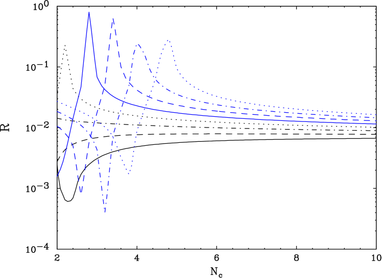
Figure 4: The renormalized difference ${\cal R}=\frac{\large{|}\rho_{2}^{Bj}-\rho_{2}^{D}\large{|}}{\large{|}\rho_{2}^{Bj}\large{|}+\large{|}\rho_{2}^{D}\large{|}}$ as a function of $N_{c}$ for various values of $N_{f}$. The four lower lines correspond to $N_{f}=0$ (continuous line), $N_{f}=1$ (dashed line), $N_{f}=2$ (dot-dash line), $N_{f}=3$ (dotted line), and the four upper curves correspond to $N_{f}=4$ (continuous line), $N_{f}=5$ (dashed line), $N_{f}=6$ (dot-dash line), $N_{f}=7$ (dotted line).

$\cal R$ is plotted in fig. 4 as a function of $N_{c}$ for various values of $N_{f}$, and in fig. 5, as a function of $N_{f}$, for various values of $N_{c}$. In general, $\cal R$ is of order $1\%$! The only occasions where the relative difference ${\cal R}$ is not small (the peaks raising above ${\cal R}=0.1$ in fig. 4 and 5) is when both $\rho_{2}^{Bj}$ and $\rho_{2}^{D}$ are close to zero. Then they may even have opposite signs, leading to ${\cal R}=1$.

We conclude that the numerical proximity between $\rho_{2}^{D}$ and $\rho_{2}^{Bj}$ is not a direct consequence of the factorization implied by the Crewther relation (r.h.s. in eq. (35)), but of the particular numerical coefficients. While the numerical proximity of $\rho_{2}^{GLS}$ and $\rho_{2}^{Bj}$ is well understood, we do not know of any reason why $\rho_{2}^{F_{1}}$ is close to $\rho_{2}^{Bj}$. It is tempting to think that there is a deeper reason for the numerical proximity, and that higher order ECH coefficients ($\rho_{i}$ for $i>2$) for different quantities are also close. In this respect it will also be interesting to know the fundamental reason why $\rho_{2}^{V}$ is so different than $\rho_{2}$ for the other space-like quantities.

Next we discuss the relation between the assumption that $\rho_{i}$ for different observables are close to one another, and the work by Brodsky and Lu [18] on commensurate-scale relations between observables. In [18] (see also [20]) it was suggested to express one effective charge ($x_{b}$) in terms of another ($x_{a}$), and then choose the scale of $x_{a}$ according to the BLM criterion [19]. In [18] it was found that the coefficients in the expansion $x_{b}=x_{b}(x_{a})$ are both much simpler than the ones in some arbitrary scheme (like $\overline{\hbox{MS}}\,$), and are numerically small. Let us see what are the conditions for the coefficients in such an expansion to be small. We start with the expressions for two generic effective charges in some scheme:

$$x_{a}=x+r_{1}^{a}x^{2}+r_{2}^{a}x^{3}+\cdots$$ (46)

$$x_{b}=x+r_{1}^{b}x^{2}+r_{2}^{b}x^{3}+\cdots$$

and express $x_{b}$ in terms of $x_{a}$:

$$x_{b}=x_{a}+m_{1}{x_{a}}^{2}+m_{2}{x_{a}}^{3}+\cdots$$ (47)

where $m_{i}$ depend on $r_{i}^{a}$ and $r_{i}^{b}$, for instance: $m_{1}=r_{1}^{b}-r_{1}^{a}$, $m_{2}=r_{2}^{b}-r_{2}^{a}-2r_{1}^{a}(r_{1}^{a}-r_{1}^{b})$. Note that $m_{i}$ are, by definition, invariant with respect to the choice of the intermediate renormalization scheme. The next step is to use the definitions of the RG invariants (2.1), and express the coefficients of (47) in terms of $\rho_{i}^{a}$ and $\rho_{i}^{b}$. $m_{1}$ is just the difference between the values of the first invariant $\rho$ (8) for the two effective charges:

$$m_{1}=r_{1}^{b}-r_{1}^{a}=\rho^{b}-\rho^{a}\equiv\Delta,$$ (48)

and higher-order coefficients can be expressed entirely in terms of $\Delta$ and of the higher-order invariants $\rho_{i}^{a}$ and $\rho_{i}^{b}$, and depend mainly on $\Delta$ and on the differences of the coefficients $\rho_{i}$. We define $\delta_{i}=\rho_{i}^{b}-\rho_{i}^{a}$, and then,

$$m_{2} = \delta_{2}+\Delta^{2}+c\Delta$$ (49)

$$m_{3} = \frac{1}{2}\delta_{3}+\Delta(\rho_{2}^{b}+2\delta_{2})+\frac{5}{2}c\Delta^{2}+\Delta^{3}$$

$\Delta$ can be tuned by changing the scale of $x_{a}$, while the scale of $x_{b}$ is kept fixed. In particular, there are choices of scale for which $\Delta$ is small, such as the leading-order BLM scale [19, 18], which eliminates all $\beta_{0}$ terms from $\Delta$, or, simply the choice $\Delta=0$ . A small $\Delta$ is, however, not enough to guarantee small higher-order $m_{i}$ coefficients. The latter will be small only if $\delta_{i}$ are also small.

One practical conclusion from this discussion is that relating $x_{D}$, $x_{Bj}$, $x_{GLS}$ and $x_{F_{1}}$ to one another as suggested in [18] will probably lead to more accurate results than some generic scheme. However, relating any of the above to $x_{V}$ is disfavored.

This concludes our discussion on the numerical proximity of the $\rho_{2}$ coefficients for space-like effective charges. Next, we briefly discuss the possibility of applying the ‘optimized-scheme’ approach to study the infrared limit of time-like effective charges.

2.5 The reliability of the “fixed point” in $R_{e^{+}e-}$ from ECH

In this section we study further the ‘optimized scheme’ approach applied directly to the $R_{e^{+}e^{-}}$ effective charge, along the lines of ref. [1, 12]. We consider specifically the case $N_{f}=3$ at the three- and four-loops order, and try to estimate the reliability of the ECH analysis in the infrared. A deeper study of time-like quantities in the context of freezing is postponed to Sec. 4.

The ‘optimized scheme’ approach was found to be unreliable when applied directly to time-like quantities in another context, by Kataev and Starshenko [34]. They found that the ECH and PMS methods for estimating the next term in a series when applied directly to two- and three-loop series for time-like quantities such as $R_{e^{+}e^{-}}$, do not predict the correct structure of the terms that result from the analytic continuation (the situation is similar for Padé approximants). The solution of [34] is to predict the coefficients of the space-like D-function and use the exact relations (2.2) to obtain the coefficients of the time-like quantity. One will naturally expect that if PMS and ECH fail in predicting the next terms when applied directly to the time-like quantities, they should not trusted for studying the infrared limit of these quantities. Nevertheless, it may still be instructive to see what one obtains in this approach.

Considering eq. (28) one finds that the $\pi^{2}$ terms, that make the coefficients of the ECH $\beta$ function of $x_{R}$ ($\rho_{i}^{R}$) different from those of $x_{D}$ ($\rho_{i}^{D}$), are numerically significant and negative. This is the reason why the analysis in Sec. 2.2 indicates an infrared fixed point for the $x_{R}$ and not for $x_{D}$ for $N_{f}\leq 4$.

Taking as an example QCD with $N_{f}=3$, we examine the ECH $\beta$ function for the D-function and $R_{e^{+}e^{-}}$:

$$\beta=-\beta_{0}x^{2}(1+cx+\rho_{2}x^{2}+\rho_{3}x^{3}+\cdots).$$ (50)

The two loop coefficient is invariant: $c=1.778$. The three loop coefficients are $\rho_{2}^{D}\simeq 5.23$ and $\rho_{2}^{R}\simeq-11.42$, and the four loop coefficients are

$$\rho_{3}^{D}\simeq-33.39+2d_{3}$$ (51)

and

$$\rho_{3}^{R}\simeq-181.98+2d_{3}$$ (52)

where $d_{3}$, the $\overline{\hbox{MS}}\,$ four loop coefficient of the D-function, is unknown.

Next, we consider different approaches to predict $d_{3}$, and thus $\rho_{3}^{D}$ and $\rho_{3}^{R}$. In the ECH/PMS approaches for predicting the next term in a perturbative series [16, 17, 34] one assumes $\rho_{3}^{D}\simeq 0$ in order to obtain a prediction for $d_{3}$. Therefore, one cannot use an ECH/PMS prediction to calculate $\rho_{3}^{D}$. Padé Approximants (PA) [36] applied in $\overline{\hbox{MS}}\,$ predict $d_{3}=24.75$ (using the $[1/1]$ PA) and $d_{3}=16.49$ (using the $[0/2]$ PA). We note that these predictions are close to one another, and are also consistent with the ECH/PMS assumption $\rho_{3}^{D}\simeq 0$, which leads to $d_{3}=16.7$. One could alternatively try to use either PMS/ECH directly for the $R_{e^{+}e^{-}}$ (i.e. assume $\rho_{2}^{R}=0$, instead of assuming $\rho_{2}^{D}=0$) or apply the PA’s method directly for the $R_{e^{+}e^{-}}$ series. However, as we already mentioned, the resulting predictions do not agree between the different methods and do not contain the correct $\pi^{2}$ terms [34] and are therefore not reliable.

We conclude that $\rho_{3}^{D}\simeq 0$ and $\rho_{3}^{R}\simeq-150$. Thus, while the question of whether the D-function effective charge freezes for $N_{f}=3$ remains open, it is quite clear that the naive ‘optimized scheme’ approach predicts that $R_{e^{+}e^{-}}$ does: $\rho_{3}^{R}$ is large and negative. Nevertheless, if the value of $x_{R}$ at the fixed point is calculated (as the zero of the four-loop ECH $\beta$ function) using a reasonable guess for $d_{3}$, one obtains a $x_{R}^{FP}\simeq 0.19\pm 0.03$ which is compared in fig. 2 with the three-loop ECH result $x_{R}^{FP}\simeq 0.38$ (or the three-loop PMS results $x_{R}^{FP}\simeq 0.30$). We therefore conclude that the ECH (or PMS) methods fail in predicting the infrared limit of the perturbative result in this case. The reasons for this will become clear in Sec. 4.

A remark is in order concerning the Higgs decay width effective charge $x_{H}$, which is also a time-like observable, and therefore contains $\pi^{2}$ terms that result from the analytical continuation. In principle, the problem discussed above should appear in this case as well. However, contrary to the case of $x_{R}$ or $x_{\tau}$, the numerical significance of these terms in the $x_{H}$ series is rather small (compared to other contributions at the same order) and therefore our previous conclusions concerning $x_{H}$ hold.

2.6 Conclusions

We analyzed here the freezing of the QCD effective charge for various quantities by looking for a zero in the corresponding ECH (or PMS) $\beta$ function.

We found a clear distinction between time-like and space-like quantities. For several space-like quantities we found that the numerical values of the second RG invariant are quite close, especially for a small $N_{f}$. This suggests that the different quantities are closely related. It is tempting to conjecture that this will be reflected in numerical proximity of $\rho_{3}$ and higher-order coefficients of the corresponding ECH $\beta$ functions. We also expect that when perturbative freezing occurs, it will occur together for the various quantities. This is clearly true for the D-function and the Bjorken polarized sum rule, due to the Crewther relation. For other quantities, such as the Bjorken non-polarized sum rule, this is just a conjecture.

For the space-like quantities (except for the static potential) it seems possible that there is a fixed point for $N_{f}\mathrel{\mathchoice{\vbox{\offinterlineskip\halign{$\m@th\displaystyle\hfil#\hfil$\cr>\crcr\sim\crcr} }}{\vbox{\offinterlineskip\halign{$\m@th\textstyle\hfil#\hfil$\cr>\crcr\sim\crcr} }}{\vbox{\offinterlineskip\halign{$\m@th\scriptstyle\hfil#\hfil$\cr>\crcr\sim\crcr} }}{\vbox{\offinterlineskip\halign{$\m@th\scriptscriptstyle\hfil#\hfil$\cr>\crcr\sim\crcr} }}}5$, while there is no indication of freezing below $N_{f}\mathrel{\mathchoice{\vbox{\offinterlineskip\halign{$\m@th\displaystyle\hfil#\hfil$\cr<\crcr\sim\crcr} }}{\vbox{\offinterlineskip\halign{$\m@th\textstyle\hfil#\hfil$\cr<\crcr\sim\crcr} }}{\vbox{\offinterlineskip\halign{$\m@th\scriptstyle\hfil#\hfil$\cr<\crcr\sim\crcr} }}{\vbox{\offinterlineskip\halign{$\m@th\scriptscriptstyle\hfil#\hfil$\cr<\crcr\sim\crcr} }}}5$. Absence of a perturbative fixed point at the three-loop level does not necessarily mean that it does not exist. It simply means that one should consider higher-order correction to answer this question. On the other hand, presence of a fixed point at the three-loop level, does not guarantee that it will persist at higher orders.

In Sec. 3 we look for more clues for or against the relevance of perturbative freezing, by studying the Banks-Zaks expansion of these quantities.

For time-like quantities, a naive application of the PMS/ECH approach indicates a perturbative fixed point even when the corresponding space-like quantity does not freeze. On the other hand we identified an instability of the predicted effective charge value at freezing. This result is a first indication of the inconsistency of the approach, as discussed further in Sec. 4.

3 The Banks-Zaks Expansion Approach

3.1 The BZ fixed point

We start this section by summarizing the basics of the BZ expansion [8, 6, 15] for the location of the fixed point.

As is mentioned in the introduction, the BZ expansion is an expansion in $(N_{f}^{*}-N_{f})$, i.e. the “distance” from the critical value $N_{f}^{*}=16\frac{1}{2}$ down to lower values of $N_{f}$. It is convenient to use the expansion parameter [15, 6]:

$$a_{0}=\frac{8}{321}\left(16\frac{1}{2}-N_{f}\right)=\frac{16}{107}\beta_{0.}$$ (53)

Since $a_{0}$ is linear in $N_{f}$, it is straightforward to rewrite the $\beta$ function coefficients $\beta_{i}=\beta_{0}c_{i}$ as polynomials in $a_{0}$, obtaining (cf. (2), (4)-(6)):

$$c=-\frac{1}{a_{0}}+c_{1,0}=-\frac{1}{a_{0}}+\frac{19}{4}$$ (54)

and

$$c_{2}=c_{2,-1}\frac{1}{a_{0}}+c_{2,0}+c_{2,1}a_{0}$$ (55)

$$c_{3}=c_{3,-1}\frac{1}{a_{0}}+c_{3,0}+c_{3,1}a_{0}+c_{3,2}a_{0}^{2}$$ (56)

where explicit expressions for $c_{i,j}$ in $\overline{\hbox{MS}}\,$ are given in ref. [6]. The next step is to solve the equation $\beta(x)=0$, yielding an expression for $x_{FP}$. With the 2-loop $\beta$ function, one obtains:

$$x_{FP}=-\frac{1}{c}=\frac{a_{0}}{1-\left(\frac{19}{4}\right)a_{0}}$$ (57)

From (57) it is clear that $x_{FP}$ is asymptotically proportional to $a_{0}$, and therefore we look for higher-order solutions $x_{FP}$, in the form of a power expansion in $a_{0}$:

$$x_{FP}=a_{0}(1+u_{1}a_{0}+u_{2}a_{0}^{2}+\cdots).$$ (58)

Assuming that a fixed point exists, one then substitutes (58) in the equation $\beta(x)=0$, finding that $u_{1}$ is fully determined by the 3-loop coefficient of the $\beta$ function, $u_{2}$ – by the 4-loop coefficient, etc. The formulae for the first three $u_{i}$-s are:

$$u_{1} = c_{1,0}+c_{2,-1}$$

$$u_{2} = c_{1,0}^{2}+2c_{2,-1}^{2}+3c_{1,0}c_{2,-1}+c_{2,0}+c_{3,-1}$$

$$u_{3} = 3c_{2,0}c_{1,0}+4c_{2,0}c_{2,-1}+4c_{1,0}c_{3,-1}+c_{1,0}^{3}+6c_{1,0}^{2}c_{2,-1}$$ (59)

$$+10c_{1,0}c_{2,-1}^{2}+c_{4,-1}+5c_{2,-1}c_{3,-1}+5c_{2,-1}^{3}+c_{2,1}+c_{3,0}$$

$u_{1},u_{2},\cdots$ depend on the renormalization scheme. One may be interested in studying the fixed point in some other scheme, related to the original one by

$$y=x(1+r_{1}x+r_{2}x^{2}+\cdots).$$ (60)

In particular, one may be interested in the fixed point in some physical scheme, in which case $y$ is an effective charge corresponding to some measurable quantity. In order to obtain the appropriate expansion for the location of the fixed point $y_{FP}$ in the new scheme, one first writes the coefficients $r_{i}$ as polynomials in $a_{0}$:

$$r_{i}=r_{i,0}+r_{i,1}a_{0}+\cdots+r_{i,i}a_{0}^{i}.$$ (61)

Next, one substitutes (61) and (58) in eq. (60), obtaining

$$y_{FP}=a_{0}(1+w_{1}a_{0}+w_{2}a_{0}^{2}+\cdots)$$ (62)

where

$$w_{1} = u_{1}+r_{1,0}$$

$$w_{2} = u_{2}+2r_{1,0}u_{1}+r_{2,0}+r_{1,1}$$

$$w_{3} = u_{3}+2r_{1,0}u_{2}+2r_{1,1}u_{1}+3r_{2,0}u_{1}+r_{1,0}u_{1}^{2}+r_{2,1}+r_{3,0}$$ (63)

It is important to note that the coefficients $w_{i}$ for a given effective charge $y$ are free from any renormalization scheme ambiguities [15], as scheme dependence cancels out between the $u_{i}$ and $r_{i}$ terms. This is expected on general grounds, since both $y_{FP}$ and $a_{0}$ in eq. (62) are physical quantities. This invariance can also be understood considering another possibility of obtaining the BZ coefficients: as a first step one calculates the $\rho_{i}$ renormalization scheme invariants (2.1) of the required effective charge. One then writes the coefficients $\rho_{i}$ as series in $a_{0}$, similarly to (55) and (56), with the only difference that here also $\rho_{i,i}$ terms appear, for instance:

$$\rho_{2}=\rho_{2,-1}\frac{1}{a_{0}}+\rho_{2,0}+\rho_{2,1}a_{0}+\rho_{2,2}a_{0}^{2}$$ (64)

Finally, one calculates the BZ expansion for the value of $x_{FP}^{\hbox{\it\footnotesize eff}}$, directly from the ECH $\beta$ function $\beta(x^{\hbox{\it\footnotesize eff}})=-\beta_{0}\left(x^{\hbox{\it\footnotesize eff}}\right)^{2}\left[1+cx^{\hbox{\it\footnotesize eff}}+\rho_{2}\left(x^{\hbox{\it\footnotesize eff}}\right)^{2}+\rho_{3}\left(x^{\hbox{\it\footnotesize eff}}\right)^{3}+\cdots\right]$, similarly to the way eq. (3.1) was obtained for the $\overline{\hbox{MS}}\,$ $\beta$ function. The resulting BZ series is exactly equal to the one obtained in (3.1) using the BZ expansion in $\overline{\hbox{MS}}\,$ as an intermediate step.

3.2 The BZ Expansion in $\overline{\hbox{MS}}\,$

Before using the BZ approach to study perturbative freezing for effective charges we consider the expansion in $\overline{\hbox{MS}}\,$, where the coefficients of the $\beta$ function are given by eqs. (2) and (4) through (6). We are interested the range $0\leq N_{f}<16\frac{1}{2}$, in which there is asymptotic freedom. We note that $c$ is negative (leading to a fixed point at the two loop order) only for $N_{f}>8.05$; $c_{2}$ is negative only for $N_{f}>5.84$, and $c_{3}$ is never negative. This makes it clear that the $\overline{\hbox{MS}}\,$ coupling is not expected to freeze within the 4-loop calculation for $N_{f}\leq 5$.

In this situation we expect the BZ expansion to break down at $a_{0}\simeq 0.26$ (corresponding to $N_{f}=6$). The coefficients of the BZ expansion are obtained directly from eq. (3.1),

$$x_{FP}^{\tiny\hbox{$\overline{\hbox{MS}}\,$}}=a_{0}+\frac{11675}{10272}\,{a_{0}}^{2}+\,\left(\frac{145645559}{17585664}+\frac{5335}{428}\,\zeta(3)\right){a_{0}}^{3}$$

$$+\,\left(-{\frac{92177206455497}{1083839643648}}-{\frac{587191201}{13189248}}\,\zeta(3)+c_{4,-1}\right){a_{0}}^{4}$$

and numerically,

$$x_{FP}^{\tiny\hbox{$\overline{\hbox{MS}}\,$}}={a_{0}}+1.1366\,{a_{0}}^{2}+23.2656\,{a_{0}}^{3}+\left(-138.5630+c_{4,-1}\right){a_{0}}^{4}.$$ (66)

We see that the series is indeed ill behaved. For example, at $a_{0}=0.26$, the first three terms are roughly: $0.26$, $0.0768$, $0.409$. In fact, the series seems to break down well above $N_{f}\sim 6$, but using only three terms it is difficult to estimate exactly where.

We conclude that at least for $N_{f}\leq 6$ the $\overline{\hbox{MS}}\,$ coupling does not freeze, and that the “Landau pole” behavior of the 1-loop coupling in the infrared, persists in $\overline{\hbox{MS}}\,$ when higher-order corrections are taken into account. But is this conclusion true to all orders? We think that the answer is positive: since the BZ expansion in $\overline{\hbox{MS}}\,$ seems to break-down already at the order ${\cal O}(a_{0}^{3})$, it is hard to imagine how higher-order corrections could alter the situation. Still, it would be interesting to know how the BZ series behaves at higher orders.

One approach [27] is to use the information that can be obtained on the $\overline{\hbox{MS}}\,$ $\beta$ function at higher-orders is from the large-$N_{f}$ limit. From the ${\cal O}(1/N_{f})$ terms calculated in [27] one can obtain all the ${\cal O}(1/a_{0})$ terms, denoted by $c_{i,i-1}$ (cf. (54) - (56)). In ref. [27] it was found that they are small, and that their effect on the value of the fixed point (and thus also on the question of its existence) is small.

Another possibility is to use PA’s [36] to estimate higher-order coefficients, and use them to calculate higher-order terms in the BZ expansion. Such an effort is now under way [37].

3.3 BZ Expansion for Time-like Quantities

In Sec. 2 we found that the ‘optimized scheme’ approach does not give reliable results for the effective charge at freezing when applied directly to time-like quantities. As we show in Sec. 4, a consistent description of freezing for $R_{e^{+}e^{-}}$ or $R_{\tau}$ exists only when the space-like D-function freezes, and then the infrared limits are expected to be the same for all three quantities:

$$D(0)=R_{e^{+}e^{-}}(0)=R_{\tau}(0).$$ (67)

This is a direct consequence of the expected analyticity structure of the D-function, which indeed holds when perturbative freezing occurs.

The ‘optimized scheme’ approach, in general, does not obey this requirement, since the terms that are related to the analytical continuation from space-like to time-like momentum, change the ECH (or PMS) $\beta$ function (see eq. (28)). Fig. 2 shows that the resulting difference between the values of the effective charges at freezing are insignificant above $N_{f}=8$. However, for $N_{f}\mathrel{\mathchoice{\vbox{\offinterlineskip\halign{$\m@th\displaystyle\hfil#\hfil$\cr<\crcr\sim\crcr} }}{\vbox{\offinterlineskip\halign{$\m@th\textstyle\hfil#\hfil$\cr<\crcr\sim\crcr} }}{\vbox{\offinterlineskip\halign{$\m@th\scriptstyle\hfil#\hfil$\cr<\crcr\sim\crcr} }}{\vbox{\offinterlineskip\halign{$\m@th\scriptscriptstyle\hfil#\hfil$\cr<\crcr\sim\crcr} }}}8$ these differences become larger. This can be interpreted as a sign that the three-loop results are not conclusively indicating freezing for these cases, which is true, but it is also related to the unjustified use of the ECH/PMS methods directly for time-like quantities.

The BZ approach, on the other hand, yields the same expansion for the three effective charges, the D-function, $R_{e^{+}e^{-}}$ and $R_{\tau}$, just as one expects from (67). It is straightforward to check this: from the relations between the coefficients of $R_{e^{+}e^{-}}$ (2.2) (or $R_{\tau}$ (31)) and those of the D-function, it is easy to obtain the relation between the corresponding coefficients of the different powers of $a_{0}$ for the two quantities, namely $r_{i,j}$ and $d_{i,j}$ (or $\tau_{i,j}$ and $d_{i,j}$). The substitution of $r_{i,j}$ (or $\tau_{i,j}$) in terms of $d_{i,j}$ into the formulae for the BZ $w_{i}$ coefficients (eq. (3.1)), gives the same $w_{i}$ coefficients as for the D-function. All the terms that result from the analytic continuation just cancel out between the different contributions, both for $R_{e^{+}e^{-}}$ and for $R_{\tau}$.

3.4 BZ Expansion for various quantities

In this section evaluate the coefficients in the BZ series for the fixed point in physical effective charges schemes for the various quantities discussed in Sec. 2.2.

The calculation is straightforward using eq. (3.1) and the three loop coefficients from refs. [28, 29, 30, 33, 32]. Thus we go directly to the results, followed by a discussion. In the next section we study the implications of the Crewther relation between $x_{D}$ and $x_{Bj}$ on the BZ expansion. Note that the ${\cal O}(a_{0}^{4})$ coefficients cannot be explicitly calculated due to the lack of both the 5-loop coefficients of the $\beta$ function and the 4-loop coefficients of the series for the different observables.

1) For the polarized Bjorken sum rule:

$$x_{FP}^{Bj}={a_{0}}+{\frac{753}{3424}}\,{a_{0}}^{2}+\left({\frac{5930095}{17585664}}-{\frac{275}{214}}\,\zeta_{3}\right)\,{a_{0}}^{3}$$

$$+\left(-\frac{18602593666427}{361279881216}-{\frac{9470237}{137388}}\,\zeta_{3}-{\frac{535}{8}}\,\zeta_{5}+c_{4,-1}+k_{3,0}\right)\,{a_{0}}^{4}$$

where $k_{3,0}$ is the 4-loop Bjorken polarized sum rule coefficient at $N_{f}=16\frac{1}{2}$, as in the general definition in eq. (61). The numerical results are:

$$x_{FP}^{Bj}={a_{0}}+0.2199\,{a_{0}}^{2}-1.2075\,{a_{0}}^{3}+\left(-203.6939+c_{4,-1}+k_{3,0}\right)\,{a_{0}}^{4}$$ (69)

2) For the non-polarized Bjorken sum rule:

$$x_{FP}^{F_{1}}={a_{0}}-{\frac{4589}{10272}}\,{a_{0}}^{2}+\left({\frac{425842061}{52756992}}+{\frac{30809}{963}}\,\zeta_{3}-{\frac{805}{18}}\,\zeta_{5}\right)\,{a_{0}}^{3}$$

$$+\left(-{\frac{38886699582523}{361279881216}}-{\frac{327376259}{2198208}}\,\zeta_{3}+{\frac{2966545}{61632}}\,\zeta_{5}+c_{4,-1}+f_{3,0}\right)\,{a_{0}}^{4}$$

or

$$x_{FP}^{F_{1}}={a_{0}}-0.4467\,{a_{0}}^{2}+0.1551\,{a_{0}}^{3}+\left(-236.7461+c_{4,-1}+f_{3,0}\right)\,{a_{0}}^{4}$$ (71)

3) For the GLS sum rule:

$$x_{FP}^{GLS}=a_{0}+\frac{753}{3424}a_{0}^{2}+\left(\frac{239442925}{52756992}-\frac{3355}{321}\zeta_{3}\right)a_{0}^{3}$$

$$+\left(-\frac{5706068695529}{120426627072}-\frac{535}{8}\zeta_{5}-\frac{171229447}{2198208}\zeta_{3}+c_{4,-1}+l_{3,0}\right)a_{0}^{4}$$

or

$$x_{FP}^{GLS}={a_{0}}+0.2199\,{a_{0}}^{2}\,-8.02495{a_{0}}^{3}+\left(-210.3609+c_{4,-1}+l_{3,0}\right)\,{a_{0}}^{4}$$ (73)

4) For the vacuum polarization D-function (and therefore, according to Sec. 3.3, also for $R_{e^{+}e^{-}}$ and $R_{\tau}$):

$$x_{FP}^{D}={a_{0}}+{\frac{4177}{3424}}\,{a_{0}}^{2}+\left({\frac{31250575}{17585664}}-{\frac{275}{214}}\,\zeta_{3}\right)\,{a_{0}}^{3}$$

$$+\left({\frac{81595375713359}{1083839643648}}-{\frac{3893665183}{13189248}}\,\zeta_{3}+{\frac{2675}{24}}\,\zeta_{5}+c_{4,-1}+d_{3,0}\right)\,{a_{0}}^{4}$$

or

$$x_{FP}^{D}={a_{0}}+1.2199\,{a_{0}}^{2}+0.2323\,{a_{0}}^{3}+(-164.0075+c_{4,-1}+d_{3,0})\,{a_{0}}^{4}$$ (75)

5) For the static potential:

$$x_{FP}^{V}=a_{0}-\frac{8869}{10272}\,a_{0}^{2}+\,\left(\frac{70824311}{17585664}+\frac{27}{8}\,\pi^{2}-\frac{9}{64}\,\pi^{4}-\frac{275}{214}\,\zeta_{3}\right)\,a_{0}^{3}$$

$$+\,\left(-\frac{130549250005577}{1083839643648}-\frac{322462723}{3297312}\,\zeta_{3}+c_{4,-1}+v_{3,0}-\frac{105075}{219136}\,\pi^{4}\right.$$

$$\left.+\frac{315225}{27392}\,\pi^{2}\right)\,a_{0}^{4}$$

or

$$x_{FP}^{V}=a_{0}-0.8634\,a_{0}^{2}+22.0945\,a_{0}^{3}+\,(-171.1353+c_{4,-1}+v_{3,0})\,a_{0}^{4}$$ (77)

6) For the derivative of the Higgs hadronic decay width:

$$x_{FP}^{H}=a_{0}+\frac{31363}{10272}\,a_{0}^{2}+\,\left(\frac{486174653}{52756992}-\frac{275}{214}\,\zeta_{3}\right)\,a_{0}^{3}$$

$$+\,\left(\frac{4675}{48}\,\zeta_{5}-\frac{294627948398435}{3251518930944}-\frac{982216871}{9891936}\,\zeta_{3}+c_{4,-1}\right)\,a_{0}^{4}$$

$$x_{FP}^{H}=a_{0}+3.0533\,a_{0}^{2}+7.6707\,a_{0}^{3}+\,(-108.9778+c_{4,-1})\,a_{0}^{4}$$ (79)

The conclusions are:

a) The BZ coefficients for $x_{Bj}^{FP}$, $x_{F_{1}}^{FP}$ and $x_{D}^{FP}$, are of order $1$ up to ${\cal O}(a_{0}^{3})$. Estimation of the “radius of convergence” from the first few terms is difficult, but convergence of these series is not ruled out for any positive $N_{f}$.

b) The BZ coefficients for $x_{GLS}^{FP}$, $x_{V}^{FP}$ and $x_{H}^{FP}$ are relatively large. For $x_{GLS}^{FP}$ and $x_{V}^{FP}$ it is very difficult to estimate the “radius of convergence” from the first few terms since $w_{1}$ coefficient is especially small, while $w_{2}$ is rather large. For $x_{H}^{FP}$ it seems that the series converges for $a_{0}\mathrel{\mathchoice{\vbox{\offinterlineskip\halign{$\m@th\displaystyle\hfil#\hfil$\cr<\crcr\sim\crcr} }}{\vbox{\offinterlineskip\halign{$\m@th\textstyle\hfil#\hfil$\cr<\crcr\sim\crcr} }}{\vbox{\offinterlineskip\halign{$\m@th\scriptstyle\hfil#\hfil$\cr<\crcr\sim\crcr} }}{\vbox{\offinterlineskip\halign{$\m@th\scriptscriptstyle\hfil#\hfil$\cr<\crcr\sim\crcr} }}}0.36$, corresponding to $N_{f}\mathrel{\mathchoice{\vbox{\offinterlineskip\halign{$\m@th\displaystyle\hfil#\hfil$\cr>\crcr\sim\crcr} }}{\vbox{\offinterlineskip\halign{$\m@th\textstyle\hfil#\hfil$\cr>\crcr\sim\crcr} }}{\vbox{\offinterlineskip\halign{$\m@th\scriptstyle\hfil#\hfil$\cr>\crcr\sim\crcr} }}{\vbox{\offinterlineskip\halign{$\m@th\scriptscriptstyle\hfil#\hfil$\cr>\crcr\sim\crcr} }}}2$.

c) Clearly, $w_{2}$ for $x_{GLS}^{FP}$ is large due to the three loop light-by-light term that makes the only difference (cf. (20)) between the GLS sum rule and the Bjorken polarized sum rule, for which $w_{2}$ is small. It may be surprising at first sight that light-by-light contribution which usually just a small correction to the three loop invariant $\rho_{2}$ can make such a difference for the BZ expansion. The reason is basically the fact that the BZ expansion works around $N_{f}=16\frac{1}{2}$, where the light-by-light term is not small, being proportional to $N_{f}$. In the vacuum polarization D-function, we neglected a similar light-by-light type term. As explained in Section 2.2, the correction expected in the D-function is smaller by a factor of $(\sum_{f}Q_{f})^{2}/N_{f}$, compared to the GLS sum rule case. This term is therefore not expected to break the BZ expansion for the D-function.

d) There is a noteworthy numerical cancelation between terms containing different irrational and transcendental numbers, that is responsible for the small $w_{2}$ values. This is particularly evident for the non-polarized Bjorken sum rule, where the rational term is roughly $8.07$, the term proportional to $\zeta_{3}$ is $38.45$, and the term proportional to $\zeta_{5}$ is $-46.37$, bringing the sum to about $0.155$! Note that the case of the non-polarized Bjorken sum rule is special both in the fact that the ${\cal O}(a_{0}^{3})$ coefficient in the BZ expansion already contains a $\zeta_{5}$ term, and in large cancelation between irrational numbers that occurs there.

e) In $x_{H}^{FP}$, which is a time-like quantity, all the $\pi^{2}$ terms that are related to the analytical continuation from space-like to time-like momentum that appear in the perturbative coefficients $h_{i}$ cancel out in the formula for the BZ series. This is in accordance with Sec. 3.3.

3.5 The BZ Expansion and the Crewther Relation

In this section we study the consequences of the Crewther relation [21] (see section 2.3) for the BZ expansions for the Bjorken sum rule and the vacuum polarization D-function.

The first observation is that the Crewther relation can be used to evaluate the difference between the yet unknown ${\cal O}(a_{0}^{4})$ coefficients in the BZ expansion of the two observables. This observation is based on the fact that from the third relation in (2.3) one can obtain $k_{3,0}-d_{3,0}$, the exact the difference between the 4-loop coefficients of the Bjorken sum rule and the vacuum polarization function at $N_{f}=16\frac{1}{2}$: by substituting $\beta_{0}=0$ the only unknown, namely $S_{3}$, is eliminated. The result is:

$$k_{3,0}-d_{3,0}=\frac{3439187}{27648}-\frac{257719}{1152}\zeta_{3}+\frac{535}{3}\zeta_{5}\simeq 40.393$$ (80)

Knowing $k_{3,0}-d_{3,0}$ we look again at eqs. (69) and (75). If the BZ expansion for the location of the fixed point converges for both observables, then both ${\cal O}(a_{0}^{4})$ coefficients should be small. Thus also their difference should also be small. And indeed, using (80) this difference can be calculated directly, to give:

$$w_{3}^{Bj}-w_{3}^{D}=-\frac{83797183}{35171328}+\frac{275}{107}\zeta_{3}\simeq 0.70686.$$ (81)

Thus the Crewther relation is consistent with a very small ${\cal O}({a_{0}}^{4})$ coefficient in the BZ expansions for both the D-function and the polarized Bjorken sum rule, with the caveat that it is also consistent with a common large contribution for both quantities.

Another (related) observation is that thanks to the conformal Crewther relation at the fixed point (41), the BZ coefficients of the vacuum polarization D-function can be calculated directly from those of the Bjorken polarized sum rule, and vice versa.

The BZ expansion of the D-function can be obtained from that of the Bjorken sum rule in two ways. In the first, one writes down the $d_{i}$ coefficients in terms of the $k_{i}$ using (2.3). Then one uses eq. (3.1) to calculate the BZ coefficients, where one finds that all the $S_{i}$ terms just cancel out, to obtain:

$$w_{1}^{D} = w_{1}^{Bj}+\frac{3}{4}C_{f}$$ (82)

$$w_{2}^{D} = w_{2}^{Bj}+\frac{3}{2}w_{1}^{Bj}C_{f}+\frac{9}{16}C_{f}^{2}$$

The second way is by first calculating the BZ expansion for the Bjorken sum rule, using eq. (3.1), as in (3.4), and then substituting the entire series into the conformal Crewther relation (41), and finally expanding the rational polynomial again in terms of $a_{0}$. The two methods are equivalent order by order.

The practical implication of this is the following: if the BZ series indeed converges fast, then the rational polynomial one gets by substituting the BZ series for the D-function in the conformal Crewther relation (41) should itself be numerically close to the power expansion (3.4). Its higher-order coefficients should provide some rough estimate of the unknown higher-order terms. We present such an analysis in fig. 7, where we show both the straightforward BZ expansion for the vacuum polarization function, and the result of substituting the BZ expansion for the Bjorken sum rule in (41). The caveat is that the results of this analysis could be invalidated if there are higher-order effects that break the BZ expansion, and are common to the D-function and the Bjorken sum rule.

3.6 The Derivative of the $\beta$ function

Following ref. [6] we now consider the derivative of the $\beta$ function at the fixed point, defined by:

$$\gamma\equiv\left.\frac{d\beta(x)}{dx}\right|_{x=x_{FP}}=-\beta_{0}x_{FP}\left[2+3cx_{FP}+4c_{2}\left(x_{FP}\right)^{2}+\cdots\right]$$ (83)

From refs. [2, 6] we adopt the following form for the $\beta$ function:

$$\frac{\beta_{0}}{\beta(x)}=-\frac{1}{x^{2}}+\frac{c}{x}-\frac{1}{\hat{\gamma}(x_{FP}-x)}+H(x)$$ (84)

where $H(x)$ is a power series in the coupling $H(x)=H_{0}+H_{1}x+\cdots$, and $\hat{\gamma}=\gamma/\beta_{0}$. $\gamma$ is called a “critical exponent” since it determines the rate at which the coupling approaches the fixed point according to

$$x-x_{FP}=\left(Q^{2}/\Lambda^{2}_{\hbox{\it\footnotesize eff}}\right)^{\gamma}$$ (85)

where $\Lambda_{\hbox{\it\footnotesize eff}}$ is the observable-dependent QCD scale [6].

It is well known that $\gamma$ is independent of the renormalization scheme, so long as the transformations relating the different schemes are non-singular (see ref. [35] and appendix B in ref. [6] and references therein).

It is straightforward to obtain the BZ expansion for $\hat{\gamma}$ by substituting eq. (58) in eq. (83) and expanding in powers of $a_{0}$. The result is:

$$\hat{\gamma}=a_{0}\left(1+g_{1}a_{0}+g_{2}{a_{0}}^{2}+\cdots\right)$$ (86)

where

$$g_{1}=c_{1,0}$$

$$g_{2}=c_{1,0}^{2}-c_{3,-1}-c_{2,-1}^{2}$$

$$g_{3}=c_{1,0}^{3}-2c_{4,-1}-c_{3,0}-4c_{2,-1}^{3}-2c_{2,0}c_{2,-1}$$ (87)

$$-4c_{1,0}c_{3,-1}-5c_{1,0}c_{2,-1}^{2}-6c_{2,-1}c_{3,-1}$$

The coefficients $g_{i}$ can be proven to be universal [15], in the sense that they are the same for any physical quantity, in agreement with the expectation that $\gamma$ is independent of the renormalization scheme in which the $\beta$ function is defined.

We now turn to the results. The BZ expansion for $\hat{\gamma}$ gives:

$$\hat{\gamma}=a_{0}+\frac{19}{4}{a_{0}}^{2}+\left(\frac{633325687}{105513984}-\frac{5335}{428}\zeta_{3}\right){a_{0}}^{3}+$$

$$\left(\frac{43834503808535}{270959910912}+\frac{590624393}{6594624}\zeta_{3}-2c_{4,-1}\right){a_{0}}^{4}$$ (88)

and finally,

$$\hat{\gamma}=a_{0}+4.75{a_{0}}^{2}-8.89129{a_{0}}^{3}+(269.43288-2c_{4,-1}){a_{0}}^{4}$$ (89)

According to ref. [6], the divergence of the $\gamma$ series is not so bad to exclude the possibility of a perturbative fixed point for the physical case of $a_{0}=0.36$ ($N_{f}=2$). We doubt this assertion, since the values the different terms in this case are: 1, 1.71, -1.15. Even for $a_{0}=0.26$ ($N_{f}=6$) one obtains a rather slowly converging series, with the different terms contributing as follows: 1, 1.24, -0.6.

If we use Padé approximants (PA’s) to estimate the unknown ${\cal O}(a_{0}^{4})$ term, we obtain a very inconsistent result. The $[2/1]$ PA gives:

$$g_{3}^{[1/2]PA}=-192.494$$ (90)

while the $[1/2]$ PA gives

$$g_{3}^{[2/1]PA}=16.982.$$ (91)

The difference between the two PA predictions above provides an estimate of the uncertainty that we have assuming that $g_{4}$ is close to zero. We therefore disagree with the assertion of [6] that a reasonable estimate for $c_{4,-1}$ can be obtained from the assumption that $g_{3}=0$.

It is interesting that the $g_{i}$-s are the same, not only for physical schemes, but also for $\overline{\hbox{MS}}\,$, even though the $\overline{\hbox{MS}}\,$ coupling is unphysical.

3.7 Conclusions

The main question one would like to answer is at what $N_{f}$ does the BZ expansion break down. Unfortunately, three terms in the expansion are not quite enough to provide a definite answer. In order to measure the convergence of the BZ expansion, we study the $N_{f}$ dependence of the ratio of the ${\cal O}({a_{0}}^{3})$ term and the partial-sum:

$$\frac{w_{2}{a_{0}}^{3}}{x_{FP}}=\frac{w_{2}{a_{0}}^{3}}{a_{0}+w_{1}{a_{0}}^{2}+w_{2}{a_{0}}^{3}}.$$ (92)

$w_{2}{a_{0}}^{3}/x_{FP}$ provides some rough measure of the convergence of a series: a divergent series where all the terms are equal and positive yields a ratio of $1/3$ above. If the signs oscillate, it yields $1$. This ratio is presented in fig. 6 for the various BZ series. It is evident that the BZ expansion behaves differently for different physical quantities: while the expansion for value of the effective-charge at freezing seems to converge for any $N_{f}$ for the polarized and non-polarized Bjorken sum rules and for the vacuum polarization D-function, it breaks down early for the GLS effective-charge (due to the light-by-light type terms), for the hadronic Higgs decay width effective-charge, for the static potential effective-charge and for the critical exponent $\gamma$. It seems that the BZ expansion is reliable down to $N_{f}=12$ in all cases, a point we shall come back to below.

We conclude this section by comparing the picture one obtains for perturbative freezing from the two approaches studied, namely, finding zeros of the $\beta$ function in an ‘optimized scheme’, and the BZ expansion. As a representative example, we choose the vacuum polarization D-function, and show in fig. 7 the value of the effective charge at freezing, as calculated by the ECH and PMS methods, together with the results from the BZ expansion. For the latter, we show both the result of a direct calculation (75) and the one obtained from the BZ expansion for the Bjorken sum rule using the conformal Crewther relation.

We interpret the difference between the ECH and PMS results, as an intrinsic uncertainty of the ‘optimized scheme’ approach in this context. Similarly, we interpret the deviation between the two BZ results as a measure of the intrinsic uncertainty of the BZ approach, related to the fact that we are using a power expansion in $a_{0}$, rather that a more generic function of $a_{0}$.

From the comparison of the two approaches for calculating $x_{D}^{FP}$, i.e. ECH/PMS vs BZ, we conclude that for $N_{f}\mathrel{\mathchoice{\vbox{\offinterlineskip\halign{$\m@th\displaystyle\hfil#\hfil$\cr>\crcr\sim\crcr} }}{\vbox{\offinterlineskip\halign{$\m@th\textstyle\hfil#\hfil$\cr>\crcr\sim\crcr} }}{\vbox{\offinterlineskip\halign{$\m@th\scriptstyle\hfil#\hfil$\cr>\crcr\sim\crcr} }}{\vbox{\offinterlineskip\halign{$\m@th\scriptscriptstyle\hfil#\hfil$\cr>\crcr\sim\crcr} }}}6$, the three-loop result can lead to a perturbative fixed point – as shown in fig. 7, the two methods agree, and predict a relatively small effective coupling in the infrared limit: $x\mathrel{\mathchoice{\vbox{\offinterlineskip\halign{$\m@th\displaystyle\hfil#\hfil$\cr<\crcr\sim\crcr} }}{\vbox{\offinterlineskip\halign{$\m@th\textstyle\hfil#\hfil$\cr<\crcr\sim\crcr} }}{\vbox{\offinterlineskip\halign{$\m@th\scriptstyle\hfil#\hfil$\cr<\crcr\sim\crcr} }}{\vbox{\offinterlineskip\halign{$\m@th\scriptscriptstyle\hfil#\hfil$\cr<\crcr\sim\crcr} }}}0.3$. We emphasize again that a zero in the truncated ECH/PMS $\beta$ can be easily washed out by higher order corrections. An extreme example is provided by the Higgs decay width effective charge, for which at the 3-loop order it seems that there is a reliable fixed point, but in fact the perturbative series breaks down.

The fact that various (space-like) effective charges run according to a very similar RG equation (at least up to 3-loops order) suggests that perturbative freezing will occur together and therefore that perturbative freezing at high enough order can be indicative for the existence of a fixed point in the full theory.

The BZ expansions for the D-function, the polarized and the non-polarized Bjorken sum rules show fast convergence up to order ${\cal O}(a_{0}^{3})$. The Crewther relation is consistent with a small ${\cal O}(a_{0}^{4})$ coefficient for the D-function and the polarized Bjorken sum rule, but it is also consistent with a common large contribution at order ${\cal O}(a_{0}^{4})$ for both quantities. From the Crewther relation it is clear that if one of these quantities freezes, so does the other.

An early break-down of the BZ expansion for physical quantities was identified for the critical exponent $\gamma$, for the static potential, for the derivative of the Higgs decay width and for the GLS sum rule.

If we assume that existence of a genuine fixed point will be realized in a perturbative manner, then we should expect convergence of the BZ expansion for any (infra-red finite) physical quantity. Using fig. 6, this leads to a prediction that

$$N_{f}^{crit}\mathrel{\mathchoice{\vbox{\offinterlineskip\halign{$\m@th\displaystyle\hfil#\hfil$\cr>\crcr\sim\crcr} }}{\vbox{\offinterlineskip\halign{$\m@th\textstyle\hfil#\hfil$\cr>\crcr\sim\crcr} }}{\vbox{\offinterlineskip\halign{$\m@th\scriptstyle\hfil#\hfil$\cr>\crcr\sim\crcr} }}{\vbox{\offinterlineskip\halign{$\m@th\scriptscriptstyle\hfil#\hfil$\cr>\crcr\sim\crcr} }}}12.$$ (93)

This result agrees with the results of Appelquist et al. [10], which are based on non-perturbative calculations and also with lattice simulations they refer to. On the other hand, it contradicts the results other lattice simulations [9].

Although this is outside the main subject of this paper, we emphasize again a nice feature of the perturbative expansions in QCD, that was noticed in two different occasions in the previous sections. This is the idea that the strong numerical cancelation between different irrational numbers (in QCD these are the $\zeta_{i}$ terms) is usually not accidental and most likely provides an indication of some yet unknown deep relation that is encoded in the perturbative coefficients. Such a cancelation was found in the difference between the second RG invariants of the D-function and of the Bjorken polarized sum rule, as well as in the ${\cal O}(a_{0}^{3})$ term in the BZ expansion for the non-polarized Bjorken sum rule.

4 Analytic continuation and time-like quantities

4.1 The D-function and $R_{e^{+}e^{-}}$

In this section we concentrate on the vacuum polarization D-function and the time-like observables that are related to it through dispersion relations: $R_{e^{+}e^{-}}$ and $R_{\tau}$.

The three loop analysis [1, 12], based on the $\beta$ function in an ‘optimized scheme’, as briefly outlined in Sections 2.1 and 2.2, suggests that the D-function effective charge does not freeze for $N_{f}\leq 4$, while the related time-like quantities do. The differences between the values of the time-like and space-like effective charges at freezing become significant already at $N_{f}\mathrel{\mathchoice{\vbox{\offinterlineskip\halign{$\m@th\displaystyle\hfil#\hfil$\cr<\crcr\sim\crcr} }}{\vbox{\offinterlineskip\halign{$\m@th\textstyle\hfil#\hfil$\cr<\crcr\sim\crcr} }}{\vbox{\offinterlineskip\halign{$\m@th\scriptstyle\hfil#\hfil$\cr<\crcr\sim\crcr} }}{\vbox{\offinterlineskip\halign{$\m@th\scriptscriptstyle\hfil#\hfil$\cr<\crcr\sim\crcr} }}}8$. On the other hand, in the framework of the BZ expansion, the time-like and space-like quantities have the same expansion for the value of the effective charge at freezing. In the following sections we shall examine this issue on a deeper level. We will show that it is inconsistent to discuss perturbative freezing of $x_{R}$ (or $x_{\tau}$) when the corresponding space-like effective charge has a “Landau-pole”. We will also explain that the terms that are related to the analytical continuation are not supposed to change the value of the effective charge at freezing, i.e. $x_{R}(0)=x_{\tau}(0)=x_{D}(0)$, provided $x_{D}(0)$ is well defined.

We start by recalling [26] the analyticity properties of the D-function and the relations between the D-function and $R_{e^{+}e^{-}}$. From the optical theorem

$$R_{e^{+}e^{-}}(s)=\frac{1}{\pi}{\rm Im}\{\Pi(-s)\}$$ (94)

where $\Pi(Q^{2})$ is defined in (21) and $s>0$ is a time-like momentum. From causality one expects that the only singularities of $\Pi(Q^{2})$ are on time-like axis, i.e. on the negative real axis: $Q^{2}=-s$ with $s>0$. The spectral density function, $\beta_{R}(s)$ is defined by

$$\beta_{R}(s)=s\frac{dx_{R}}{ds}$$ (95)

Clearly $\beta_{R}$ is also the $\beta$ function for the coupling $x_{R}$. Differentiating (94) one obtains a similar relation between $\beta_{R}$ and the space-like D-function effective charge (22),

$$\beta_{R}(s)=-\frac{1}{\pi}{\rm Im}\{x_{D}(-s)\}$$ (96)

Based on the above, one can express the D-function as a dispersive integral over $R_{e^{+}e^{-}}$,

$$x_{D}(Q^{2})=-\int_{0}^{\infty}ds\frac{\beta_{R}(s)}{s+Q^{2}}=Q^{2}\int_{0}^{\infty}ds\frac{x_{R}(s)}{(s+Q^{2})^{2}}.$$ (97)

The relations between the coefficients of the corresponding effective charges $x_{R}$ and $x_{D}$ (2.2) are directly obtainable from (97), as explained in ref. [26].

The inverse relation is:

$$R_{e^{+}e^{-}}(s)=\frac{1}{2\pi i}\int^{s+i\epsilon}_{s-i\epsilon}ds^{\prime}\frac{d\Pi(-s^{\prime})}{ds^{\prime}}=-\frac{1}{2\pi i}\int_{s-i\epsilon}^{s+i\epsilon}ds^{\prime}\frac{D(-s^{\prime})}{s^{\prime}},$$ (98)

where the integration contour lies in the region of analyticity of $D(-s)$, that is, around the cut ${\rm Re}\{s^{\prime}\}>0$. The contour can also be deformed to a circle,

$$R_{e^{+}e^{-}}(s)=\frac{1}{2\pi i}\oint_{|s^{\prime}|=s}\frac{ds^{\prime}}{s^{\prime}}D(-s^{\prime}).$$ (99)

Relations (98) and (99) are also true for the corresponding effective charges, i.e. replacing $R_{e^{+}e^{-}}$ and $D(Q^{2})$ by $x_{R}$ and $x_{D}$, respectively, for instance,

$$x_{R}(s)=\frac{1}{2\pi i}\oint_{|s^{\prime}|=s}\frac{ds^{\prime}}{s^{\prime}}x_{D}(-s^{\prime}).$$ (100)

It is clear from eq. (100) that the infrared limit of $R_{e^{+}e^{-}}(s)$ equals that of the D-function if the latter exists: assuming the D-function does not have an essential singularity at $s^{\prime}=0$, we have $x_{D}(-s^{\prime})\longrightarrow x_{D}(0)$ and thus for small enough $s$ the only singularity within the integration contour is the simple pole at the origin. From Cauchy’s theorem one then obtains $x_{R}(s)\longrightarrow x_{D}(0)$.

From this argument one learns that the infrared limit of the exact $R_{e^{+}e^{-}}$ equals to that of the exact D-function. But does this hold in perturbation theory? The results of the ‘optimized scheme’ approach and the BZ expansion indicate that this is a delicate question. This issue is discussed further in the following sections.

The analogous issue for $R_{\tau}$ will not be discussed in detail in this paper, but most of our results are quite general and apply to it directly, since this quantity is related to the D-function in a similar way [31]:

$$R_{\tau}(m^{2}_{\tau})=\frac{1}{2\pi i}\oint_{|x|=1}\frac{dx}{x}\left(1-2x+2x^{3}-x^{4}\right)D(-xm_{\tau}^{2})$$ (101)

Like in the $R_{e^{+}e^{-}}$ case, it can easily be shown that when $D(-xm_{\tau}^{2})=D(0)$ freezes, eq. (101) leads to an equality of the infrared limits $R_{\tau}(0)=D(0)$.

4.2 The analyticity structure of the D-function

The physical quantity which can be measured directly is the time-like $x_{R}$, or its derivative $\beta_{R}(s)$, and not the space-like effective charge $x_{D}(Q^{2})$. On the other hand, the perturbative calculation yields $x_{D}(Q^{2})$. Naively, there is no problem to obtain $\beta_{R}(s)$ from $x_{D}$ via eq. (96). This is done by analytically continuing the perturbative $x_{D}(Q^{2})$ to time-like momentum $Q^{2}={-}s$, where $s>0$, and taking the imaginary part. Alternatively, one can obtain $x_{R}(s)$ from eq. (100). Unfortunately, the analyticity structure of perturbative $x_{D}(Q^{2})$ is inconsistent with this procedure. The relations between $x_{D}$ and $x_{R}$ are based on the assumption that $x_{D}(Q^{2})$ is analytic in the entire complex $Q^{2}$ plane, excluding the negative real axis, $Q^{2}<0$. On the other hand, a 1-loop perturbative result for $x_{D}(Q^{2})$ violates causality, since it has a “Landau-pole” at positive real $Q^{2}=\Lambda_{QCD}^{2}\,$,  in addition to the cut at $Q^{2}<0$. In general, higher-order corrections to the $\beta$ function create a more complicated analyticity structure which also violates causality. Another way to see this problem is that eqs. (98) and (99) lead to different results for $x_{R}$ with the same $D$ function taken as input. This point is discussed in ref. [5].

In case of perturbative freezing, $x_{D}(Q^{2})$ is finite for any positive real $Q^{2}$. One might then be tempted to conclude that freezing saves causality. This is not necessarily the case, however, since in principle $x_{D}(Q^{2})$ could still be singular at some complex $Q^{2}$, while causality requires $x_{D}(Q^{2})$ to be analytical in the entire complex $Q^{2}$ plane, apart from the time-like axis. Thus the resolution of the causality question requires full knowledge of the $x_{D}(Q^{2})$ singularity structure. As we shall shortly demonstrate, the latter can be obtained explicitly.

Before investigating in general whether freezing saves causality, we study a specific numerical example, where we demonstrate how perturbative freezing leads to an $x_{D}(Q^{2})$ which is consistent with causality. We work with a 2-loop $\beta$ function

$$\beta(x_{D})=\frac{dx_{D}}{dt}=-\beta_{0}{x_{D}}^{2}\left(1+cx_{D}\right)$$ (102)

where $t=\ln(Q^{2}/\Lambda^{2}_{\hbox{\it\footnotesize eff}})$, and for illustration purposes we take the hypothetical case $\beta_{0}=1$ and $c=-10$.

We will see that the solution of (102) defines a unique mapping from the entire complex $Q^{2}$ plane (except the time-like axis) into a compact domain in the complex $x_{D}$ plane [38]. This domain does not contain the point $x_{D}=\infty$.

A straightforward integration of (102) yields:

$$\beta_{0}\ln(Q^{2}/\Lambda^{2}_{\hbox{\it\footnotesize eff}})=\frac{1}{x_{D}}-c\ln\left(\frac{1+cx_{D}}{x_{D}}\right)$$ (103)

In order to study the solutions of (103) in the complex plane, it is convenient to define:

$$\ln(Q^{2}/\Lambda^{2}_{\hbox{\it\footnotesize eff}})\equiv p+i\eta,$$ (104)

where $p\geq 0$ and $-\pi\leq\eta<\pi$,  and

$$x_{D}(Q^{2})\equiv r(p,\eta)+ik(p,\eta)\equiv r+ik,$$ (105)

where both $r$ and $k$ are real. Eq. (103) can then be written as two equations for the real and imaginary parts

$$\beta_{0}p\,=\,\frac{r}{r^{2}+k^{2}}-\frac{1}{2}c\ln\left(c^{2}+\frac{1+2cr}{r^{2}+k^{2}}\right)$$ (106)

and

$$\beta_{0}\eta\,=\,-\frac{k}{r^{2}+k^{2}}+c\arctan\left[k,c(r^{2}+k^{2})+r\right]$$ (107)

where $\arctan[u,v]\equiv\hbox{arg}\{u+iv\}$ takes values in $[-\pi,\pi)$.

An infrared fixed point in the two loop $\beta$ function ($c<0$) implies that for real $Q^{2}\geq 0$ eq. (103) has a real solution $0\leq x_{D}\leq({-1}/c)$. In the notation of eqs. (106) and (107) this means that for $\eta=0$ and for any $p\geq 0$ there is a solution with $k=0$ and $0\leq r\leq-1/c$. Clearly, $x_{D}$ has a cut for real $Q^{2}<0$, i.e. for $\eta=\pi$.

In order to verify that there are no other singularities in the complex $Q^{2}$ plane, we explicitly find the domain in the complex $x_{D}$ plane into which the entire $Q^{2}$ plane is mapped through (103). This is done by taking a contour around the cut and solving eqs. (106) and (107) numerically for $\Lambda^{2}_{\hbox{\it\footnotesize eff}}=1$. We choose the following contour in the $Q^{2}$ plane:

a) below the cut: $Q^{2}=-s-i\epsilon$, $0<s<\infty$, with $\epsilon=0.01$;

b) to the right of the cut: $Q^{2}=p_{0}+i\xi$, with $p_{0}=10^{-10}$ and ${-}\epsilon\leq\xi\leq\epsilon$;

c) above the cut: $Q^{2}=-s+i\epsilon$ with $0<s<\infty$.

as shown schematically in the upper part of fig. 8. The resulting contour in the $x_{D}$ plane is presented in the lower part of fig. 8. Clearly, the particular choice of the contour around the cut is arbitrary, but a contour that is closer to the cut (smaller $\epsilon$ and $p_{0}$) would correspond to an $x_{D}$ domain which is only slightly larger. We see that the entire complex $Q^{2}$ plane is mapped into a compact domain in $x_{D}$ plane. Thus there are no spurious singularities in the complex $Q^{2}$ plane and so causality is preserved.

We emphasize that the solution of eqs. (106) and (107) described by this particular mapping is not unique and there exist other branches of the solution. However, none of them corresponds to a real coupling $x_{D}$ along the positive real $Q^{2}$ axis. It is this requirement that guarantees uniqueness of the solution.

Returning to the more general case of a 2-loop $\beta$ function, we will now show that perturbative freezing alone ($c<0$) is insufficient to ensure that the analyticity structure of $x_{D}(Q^{2})$ is consistent with causality. A further condition is required, namely that $|c|>\beta_{0}$.

The solution of the RG equation at the 2-loop order (102) in the complex $Q^{2}$ plane can be written in terms of the so-called Lambert $W$ function [39], which is defined by $W(y)\exp\left[W(y)\right]=y\,$:

$$\begin{array}[]{c}\displaystyle x_{D}(Q^{2})=-\frac{1}{c}\,\,\frac{1}{1+W(z)}\\ \phantom{a}\\ \displaystyle z=-\frac{1}{c}\exp\left(-1-\beta_{0}t/c\right)=-\frac{1}{c\,e}\left(\frac{Q^{2}}{\Lambda_{\hbox{\it\footnotesize eff}}^{2}}\right)^{-\beta_{0}/c}\end{array}$$

$W(y)$ is a multi-valued function with an infinite number of branches, denoted by $W_{n}(y)$. We follow [39] as for the division of the branches and notation. The requirement that $x_{D}(Q^{2})$ is real and positive for a real positive $Q^{2}$ (at least for $Q^{2}\gg\Lambda_{\hbox{\it\footnotesize eff}}^{2}$), is sufficient to determine the relevant branch: for $c>0$ the physical branch is $W_{-1}(y)$, taking real values in the range $(-\infty,-1)$, and for $c<0$ the physical branch is the principal branch, $W_{0}(y)$, taking real values in the range $(-1,\infty)$.

We now need to check if the singularity structure of $x_{D}(Q^{2})$ in (4.2) is consistent with causality. Let us first consider the case $c>0$: $W_{-1}(y)$ has two branch points, at $y=0$ and at $y=-1/e$, which are the endpoints of two cuts stretching to $y=-\infty$.

The point at $y=0$ corresponds to $Q^{2}\longrightarrow\infty$. The point at $y=-1/e$ corresponds to

$$Q^{2}_{sing}=\Lambda^{2}_{\hbox{\it\footnotesize eff}}c^{-c/\beta_{0}}=\Lambda^{2}_{\hbox{\it\footnotesize eff}}\exp\left(-c/\beta_{0}\ln(c)\right)$$ (108)

which implies that there is a “Landau singularity” on the space-like axis. Thus for $c>0$ the singularity structure is inconsistent with causality.

For $c<0$, the physical branch $W_{0}(y)$ has only one branch point at $y=-1/e$, with a cut stretching to $y=-\infty$. In the complex $Q^{2}$ plane this corresponds to branch points, i.e. “Landau singularities”, given by (108). Two different possibilities exist:

a) $c<0$ and $|c|<\beta_{0}$. There is a pair of singularities in the complex $Q^{2}$ plane.

b) $c<0$ and $|c|>\beta_{0}$. There are no singularities in the first sheet and the perturbative solution is consistent with causality. In this case $x_{D}(Q^{2})$ maps the whole complex $Q^{2}$ plane into a compact domain in the coupling plane. The latter situation was illustrated above in the example with $\beta_{0}=1$, $c=-10$.

We will not consider here the higher-order $\beta$ function. We expect that also in this case there are regions of parameter space resulting in an analyticity structure consistent with causality, i.e. allowing the mapping of the entire complex $Q^{2}$ plane into a compact domain in the complex coupling plane. On the basis of the experience with the two-loop $\beta$ function, we conjecture that causality will be preserved by a wide subset, but not by the entire parameter space for which perturbative freezing holds. In general, the perturbative result does not have the analyticity structure implied by causality, and therefore does not obey the dispersion relation of (96) and (97). There is a way, however, to start from the perturbative $\beta$ function and impose the dispersion relation on it: this is the so-called Analytic Perturbation Theory (APT) approach, which is the subject of the next section.

4.3 Analytic perturbation theory approach

The objective of the APT approach [5, 4] is to achieve the required analyticity structure, while retaining the correct perturbative behavior in the ultraviolet region.

The technique is based on solving eqs. (106) and (107) on the negative real axis, i.e. for $\eta=-\pi$. This can be done starting with the RG equation at any order. For instance, suppose we work at the 3-loop order and define the coupling $x(Q^{2})$ in some arbitrary scheme and scale. Then $x_{D}=x+d_{1}x^{2}+d_{2}x^{3}$. The imaginary part of $x_{D}(-s)$ yields the spectral density function $\beta_{R}(s)$:

$$\beta_{R}(s) = -\frac{1}{\pi}{\rm Im}\{x_{D}(-s)\}=-\frac{1}{\pi}{\rm Im}\left\{x(-s)+d_{1}x(-s)^{2}+d_{2}x(-s)^{3}\right\}$$ (109)

$$= -\frac{1}{\pi}k(t)\left[1+2d_{1}r(t)+d_{2}\left(3{r(t)}^{2}-{k(t)}^{2}\right)\right]$$

where $x(-s)\equiv r(t)+ik(t)$, and $t=\ln(s/\Lambda^{2}_{\hbox{\it\footnotesize eff}})$, where $s$ is time-like, $s>0$ (cf. (105)).

The only case where the APT spectral function can be obtained in a closed form is for the 1-loop $\beta$ function. Substituting $c=0$ and $\eta=-\pi$ in eqs. (106) and (107), one obtains two algebraic equations for $r(s)$ and $k(s)$, whose solutions are:

$$k(t) = \frac{\beta_{0}\pi}{(\beta_{0}\pi)^{2}+(\beta_{0}t)^{2}}$$

$$r(t) = \frac{\beta_{0}t}{(\beta_{0}\pi)^{2}+(\beta_{0}t)^{2}}$$ (110)

The spectral density at this order is simply

$$\beta_{R}(t)=-\frac{1}{\pi}k(t)=-\frac{1}{\beta_{0}\left[\left(\ln(s/\Lambda^{2})\right)^{2}+\pi^{2}\right]}.$$ (111)

Integrating the spectral density yields the time-like effective charge $x_{R}$:

$$x_{R}(t)=\frac{1}{\beta_{0}\pi}\arctan\left(\pi/t\right)+\frac{1}{\beta_{0}}\theta\left(-t\right).$$ (112)

This is a positive, continuous and monotonically increasing function of $s$ for any $s>0$. Its infrared limit is $1/\beta_{0}$. In the ultraviolet region this function approaches the 1-loop perturbative result $x_{R}(s)\longrightarrow 1/(\beta_{0}t)$.

It has been recently emphasized (see the last ref. in [5]) that the results of the APT approach do not depend much on the renormalization scheme and scale. The reason for this stability (which has not been given in [5]) is rather simple to understand already from the 1-loop result: a scale or scheme transformation at this order amounts to a shift in $\Lambda$: $\Lambda\longrightarrow\tilde{\Lambda}$. It is clear that the $\pi^{2}$ term in the denominator of (111) “hides” variations in $\Lambda$ which are not too large.

In order to study the higher order terms that make the APT result different from the standard perturbative 1-loop result, we construct the expression for the spectral density $\beta_{R}$ (which is also the time-like $\beta$ function) in terms of the effective-charge $x_{R}$. The perturbative regime corresponds to $s>\Lambda^{2}$, so we can now ignore the $\theta$ function in the inversion of (112), obtaining

$$t=\frac{\pi}{\tan(\beta_{0}\pi x_{R})}$$ (113)

We then substitute (113) in (111) and obtain:

$$\beta(x_{R})=\frac{dx_{R}}{dt} = -\,\frac{\left(\tan(x_{R}\pi\beta_{0})\right)^{2}}{\beta_{0}\pi^{2}\left[1+\left(\tan(\beta_{0}\pi x_{R})\right)^{2}\right]}$$

$$\simeq -\beta_{0}\left(x_{R}^{2}-\frac{1}{3}\pi^{2}\beta_{0}^{2}\,x_{R}^{4}+\frac{2}{45}\pi^{4}\beta_{0}^{4}\,x_{R}^{6}+\cdots\right)$$

Formally we work at the 1-loop level, so the higher-order terms in the r.h.s. of (4.3) are only a part of the full higher-order result. Still, we see that solving the RG equation on the time-like axis yields an infinite series of $\pi^{2}\beta_{0}^{2}$ terms. For instance, we recognize the coefficient of the first correction, $-\beta_{0}^{2}\pi^{2}/3$, as the difference between the ECH coefficients $\rho_{2}^{D}$ and $\rho_{2}^{R}$ in eq. (28). Thus the APT approach can be viewed as a method of resumming the infinite series of terms associated with the analytical continuation.

Following [5] we construct the corresponding space-like effective coupling, which is defined through the dispersion relation (97). The integral can be performed analytically, and yields

$$x_{\hbox{\it\footnotesize APT}}(Q^{2})=\frac{1}{\beta_{0}}\left[\frac{1}{\ln\left(Q^{2}/\Lambda^{2}\right)}+\frac{\Lambda^{2}}{\Lambda^{2}-Q^{2}}\right],$$ (115)

The 1-loop APT effective coupling result (115) contains a first term that is just the 1-loop perturbative result and a second term that exactly cancels the “Landau-pole”. Since this term is a power correction, it does not alter the perturbative ultraviolet behavior.

Let us summarize the characteristics of the APT result, which are demonstrated above: by construction $x_{\hbox{\it\footnotesize APT}}(Q^{2})$ has a cut at ${\rm Re}\{Q^{2}\}<0$ and no other singularities in the complex plane, and in this sense it is appropriate to describe the D-function. Again, by construction, the APT result is consistent with the requirement that the time-like and space-like infrared limits are equal $x_{R}(0)=x_{\hbox{\it\footnotesize APT}}(0)$. At 1-loop the infrared limit value is $x_{\hbox{\it\footnotesize APT}}(0)=1/\beta_{0}$.

We stress that there is an important difference between perturbative freezing, that leads to a finite infrared limit within perturbation theory, and the APT approach, where $x_{\hbox{\it\footnotesize APT}}(Q^{2})$ is not purely perturbative, as it contains power corrections that are due to the imposed analyticity. The non-perturbative nature of the APT result is less transparent on the time-like axis, where, as we saw, the APT approach can be viewed as a method to resum the infinite series of terms that are related to the analytical continuation. All-order resummations are in general dangerous. It is well known that the perturbative series itself has a zero radius of convergence, and that it is even non Borel-summable (see, for instance, [41]). Therefore, an all-order resummation of a partial series can yield any arbitrary result. One has to be convinced that a resummation procedure yields a result that is closer to the exact one, before utilizing it. It is important to understand that analyticity alone is not enough to set the infrared limit: one can still add further power corrections which can alter the infrared limit without violating the expected analyticity structure [40].

From the 1-loop APT result it is transparent that the terms in $\beta_{R}$ which are due to the analytical continuation have nothing to do with the existence of an infrared fixed point in QCD. Still, one can use the APT result to analyze the instability found in the predictions for the fixed point in the ‘optimized-scheme’ method (Sec. 2.5). As we saw, the fixed point of the “all-order” 1-loop APT result is at $x_{R}^{FP}=1/\beta_{0}$. On the other hand, the function $\beta_{R}$ of eq. (4.3), when truncated at order $x_{R}^{4}$, has a zero at $x_{R}^{FP}=\sqrt{3}/(\pi\beta_{0})$. However, when truncated at order $x_{R}^{6}$, it does not have a non-trivial fixed point. At higher-orders, the $\beta$ function has a non-trivial zero only when the series is truncated at an even power of $x_{R}^{2}$. Moreover, the convergence of the corresponding fixed point values to the limiting “all-order” value is quite slow. For instance, the deviation at order $x_{R}^{4}$ is $45\%$, at order $x_{R}^{8}$ it is $26\%$, and at order $x_{R}^{12}$ it is $12\%$. This exercise shows that one cannot trust the value one gets by applying the ‘optimized scheme’ procedure to time-like quantities.

Until now we discussed the APT approach for the 1-loop $\beta$ function. It is interesting to see how the APT results change when higher loops are included. As in Sec. 4.2, we restrict our discussion to the 2-loop case. Starting from eq. (103) and performing analytical continuation by taking $Q^{2}=-s$ with $s>0$, we obtain:

$$\beta_{0}\ln(-s/\Lambda^{2}_{\hbox{\it\footnotesize eff}})=\frac{1}{x_{D}(-s)}-c\ln\left(\frac{1+cx_{D}(-s)}{x_{D}(-s)}\right).$$ (116)

As mentioned in the previous section, inverting this implicit relation is non-trivial. In fact, there is an infinite number of solutions for $x_{D}(-s)$:

$$\begin{array}[]{c}\displaystyle x_{D}^{n\pm}(-s)=-\frac{1}{c}\,\frac{1}{1+W_{n}(\zeta^{\pm})}\\ \phantom{a}\\ \displaystyle\zeta^{\pm}=-\frac{1}{c}\exp\left[-1-(t\pm i\pi)\beta_{0}/c\right]\end{array}$$ (117)

for any integer $n$. As explained in detail in [42], uniqueness of the APT coupling is guaranteed only if the time-like solution $x_{D}(-s)$ is obtained from the physical space-like solution in such a way that for $|Q^{2}|\gg\Lambda^{2}$ the coupling $x_{D}(Q^{2})$ is continuous for a continuous change of the phase of $Q^{2}$. From here one proceeds, just as in the 1-loop case, by taking the imaginary part $\beta_{R}=-(1/\pi){\rm Im}\{x_{D}(-s)\}$ and finally calculating $x_{\hbox{\it\footnotesize APT}}$ using (97), as in (115).

While a full description of the analytic continuation from the space-like to the time-like axis using the various branches of the Lambert W function is postponed to [42], we briefly present here some of the conclusions concerning the APT infrared limit. There are two possibilities: if $c<-\beta_{0}<0$ (the perturbative solution is consistent with causality) the APT coupling coincides with the perturbative one and the infrared limit is $x_{\hbox{\it\footnotesize APT}}(0)=x_{D}(0)=-1/c$. Otherwise, for $c>-\beta_{0}$, $x_{\hbox{\it\footnotesize APT}}(0)=1/\beta_{0}$. Note the the latter is relevant both for $-\beta_{0}<c<0$ cases, where there is a pair of complex singularities in the complex $Q^{2}$ plane, and for $c>0$ cases, where there is one space-like singularity.

5 Conclusions

In this work we investigated the possibility that there is an infrared fixed point in QCD with $N_{f}$ flavors, $0\leq N_{f}\leq 16\frac{1}{2}$, that can be identified from perturbative calculation. We examined the effective running coupling constant, defined from several QCD observables in the ‘optimized scheme’ approach and by the BZ expansion.

We showed that several different (space-like) effective-charges behave similarly to one another. This suggests that freezing occurs for all of them together and therefore that perturbative freezing may be indicative of a genuine fixed point.

In general, the ECH/PMS approach, when applied to space-like quantities at the 3-loop order indicates a possible perturbative fixed point for $N_{f}\mathrel{\mathchoice{\vbox{\offinterlineskip\halign{$\m@th\displaystyle\hfil#\hfil$\cr>\crcr\sim\crcr} }}{\vbox{\offinterlineskip\halign{$\m@th\textstyle\hfil#\hfil$\cr>\crcr\sim\crcr} }}{\vbox{\offinterlineskip\halign{$\m@th\scriptstyle\hfil#\hfil$\cr>\crcr\sim\crcr} }}{\vbox{\offinterlineskip\halign{$\m@th\scriptscriptstyle\hfil#\hfil$\cr>\crcr\sim\crcr} }}}5$. It is clear, however, that the knowledge of higher-order corrections is essential for a conclusive answer. While for some observables the BZ expansion has small coefficients suggesting that it converges down to low $N_{f}$, in other physical schemes it breaks down quite early. Assuming that existence of a fixed point means that the BZ expansion should converge for any physical quantity, we get a prediction that $N_{f}^{crit}\mathrel{\mathchoice{\vbox{\offinterlineskip\halign{$\m@th\displaystyle\hfil#\hfil$\cr>\crcr\sim\crcr} }}{\vbox{\offinterlineskip\halign{$\m@th\textstyle\hfil#\hfil$\cr>\crcr\sim\crcr} }}{\vbox{\offinterlineskip\halign{$\m@th\scriptstyle\hfil#\hfil$\cr>\crcr\sim\crcr} }}{\vbox{\offinterlineskip\halign{$\m@th\scriptscriptstyle\hfil#\hfil$\cr>\crcr\sim\crcr} }}}12$.

We emphasized a fundamental difference in QCD between the infrared behavior of quantities naturally defined for space-like and time-like momentum. We showed that perturbative freezing is a necessary (but not a sufficient) condition for consistency of perturbation theory with a causal analyticity structure. When the infrared finite perturbative coupling has a causal analyticity structure it coincides with the APT coupling.

We emphasized that freezing leads to the equality of the time-like and space-like effective couplings at the fixed point. In this context it is important to stress that the terms due to the analytical continuation in the time-like $\beta$ function are in principle not related to perturbative freezing. In the BZ expansion such terms cancel out, making it more reliable than the ‘optimized scheme’ approach, where they can lead to the appearance of spurious infrared fixed points.

Acknowledgments

E.G. would like to thank G.P. Korchemsky for very useful discussions and to the organizers of the YKIS’97 international seminar in Kyoto, in December ’97, where a part of this work was done. The authors also thank J. Ellis for comments on the manuscript. Special thanks are due to G. Grunberg for very useful discussion and for constructive criticism of the original version of the paper. This research was supported in part by the Israel Science Foundation administered by the Israel Academy of Sciences and Humanities, and by a Grant from the G.I.F., the German-Israeli Foundation for Scientific Research and Development and by the Charles Clore doctoral fellowship.

Figure 1: The second renormalization-group invariant $\rho_{2}$ as a function of the number of light flavors for various space-like (continuous lines) and time-like (dashed lines) quantities. Also shown is $c_{2}$, the second coefficient of the $\beta$ function in $\overline{\hbox{MS}}\,$ (dotted line). Note the closeness of the curves for all the space-like quantities except the static potential ($V$).

Figure 2: The values of the effective charges at the fixed point, as a function of $N_{f}$, calculated in the ECH scheme (continuous lines) at the three loop order: upper line – the space-like vacuum polarization D-function, middle line – $R_{\tau}$ and lower line – $R_{e^{+}e^{-}}$. The dashed line represents the D-function effective charge at freezing calculated in the PMS scheme at the three loop order. Also presented is the ECH result for $N_{f}=3$ at the four loop order as calculated using predicted values for $d_{3}$ (see Sec. 2.5).

Figure 3: The differences between $\rho_{2}$ values for various quantities and for the vacuum polarization D-function. Space-like quantities are plotted as continuous lines, while time-like quantities appear as dashed lines. The vertical axis is magnified $10$ times compared to fig. 1. At small $N_{f}$ all the space-like $\rho_{2}$ invariants are close to each other. For $N_{f}\approx 16\frac{1}{2}$, $\rho_{2}^{D}$ coincides with those of the related time-like quantities.

Figure 5: The renormalized difference ${\cal R}=\frac{\large{|}\rho_{2}^{Bj}-\rho_{2}^{D}\large{|}}{\large{|}\rho_{2}^{Bj}\large{|}+\large{|}\rho_{2}^{D}\large{|}}$ as a function of $N_{f}$ for various values of $N_{c}$. The four lines correspond to $N_{c}=2$ (continuous line), $N_{c}=3$ (dashed line), $N_{f}=4$ (dot-dash line), $N_{f}=5$ (dotted line).

Figure 6: The ratio of the ${\cal O}({a_{0}}^{3})$ term in the BZ expansion and the partial-sum ($w_{2}{a_{0}}^{3}/x_{FP}$) is shown for various quantities at the fixed point as a function of $N_{f}$. The dot-dashed line represents the non-polarized Bjorken sum rule effective charge.

Figure 7: $x_{FP}^{D}$ as calculated from the ECH method (continuous line) the PMS method (dashed line) and the BZ expansion at the three loop order. For the BZ expansion, both the results of a direct calculation (dot-dash line) and a calculation that uses the Bjorken sum rule and the Crewther relation (41) (dashed line) are presented.

Figure 8: The mapping of the entire complex $Q^{2}$ plane (except the negative real axis) into a compact domain in the complex coupling plane in the case of a 2-loop $\beta$ function (102), with $\beta_{0}=1$ and $c=-10$. The upper plot shows schematically the contour around the cut in the $Q^{2}$ plane as described in the text (Sec. 4.2). The lower plot shows the image of this contour in the complex coupling ($x_{D}$) plane. The two fixed points (ultraviolet, at $x_{D}=0$, and infrared, at $x_{D}=-1/c=0.1$) are denoted as squares.

References

- [1] A. C. Mattingly and P. M. Stevenson, Phys. Rev. D49,437; Phys. Rev. Lett. 69, 1320 (1992).
- [2] P. M. Stevenson, Phys. Lett. B331 (1994) 187-192.
- [3] G. Parisi and R. Petronzio, Phys. Lett. B94, (1980) 51.
- [4] Yu. L. Dokshitzer G. Marchesini and B. R. Webber, Nucl. Phys. B469 (1996) 93; G. Grunberg Power corrections and Landau singularity, hep-ph/9705290.
- [5] D.V. Shirkov On the analytic “Causal” model for the QCD running coupling, hep-ph/9708480; K. A. Milton, O. P. Solovtsova, OKHEP-97-06, Analytic perturbation theory: a new approach to the analytic continuation of the strong coupling constant alpha-s into the time-like region, hep-ph/9710316; I.L. Solovtsov and D.V. Shirkov, Phys. Rev. Lett. 79 (1997) 1209-1212, Analytic model for the QCD running coupling with universal value hep-ph/9704333; I.L. Solovtsov and D.V. Shirkov Analytic approach to perturbative QCD and renormalization scheme dependence, hep-ph/9711251.
- [6] S. A. Caveny and P. M. Stevenson, The Banks-Zaks Expansion and “Freezing” in Perturbative QCD, hep-ph/9705319;
- [7] S. J. Brodsky, C.-R. Ji, A. Pang and D. G. Robertson, Phys. Rev. D57 (1998) 245-252.
- [8] T. Banks and A. Zaks, Nucl. Phys. B196 (1982) 189.
- [9] Y. Iwasaki, Phase structure of lattice QCD for general number of flavours hep-lat/9707019 and references therein.
- [10] T. Appelquist, J. Terning and L.C.R. Wijewardhana Phys. Rev. Lett. 77 (1996) 1214-1217; M. Velkovsky, E. Shuryak QCD with large number of quarks: effects of the instanton - anti-instanton pairs, SUNY-NTG-96-37, hep-ph/9703345; V.A. Miransky and Koichi Yamawaki, Phys. Rev. D55 (1997) 5051-5066 (Erratum-ibid D56 (1997) 3768).
- [11] T. Banks, A. Casher Nucl. Phys. B169 (1980) 103.
- [12] J. Chyla, A. Kataev and S. Larin, Phys. Lett. B267 (1991) 269-276.
- [13] J. Chyla and A. Kataev, Phys. Lett. B297 (1992) 385.
- [14] S.G. Gorishny, A.L. Kataev, S.A. Larin and L.R. Surguladze, Phys. Rev D43 (1991) 1633.
- [15] G. Grunberg, Phys. Rev. D46 (1992) 2228.
- [16] G. Grunberg, Phys. Rev. D29 (1984) 2315; A. Dhar and V. Gupta, Phys. Rev. D29 (1984) 2822.
- [17] P.M. Stevenson, Phys. Rev. D23 (1981) 2916.
- [18] S.J. Brodsky and H.J. Lu, Phys. Rev. D51 (1995) 3652.
- [19] S.J. Brodsky, G.P. Lepage and P.M. Mackenzie, Phys. Rev. D28 (1983) 228;
- [20] S.J. Brodsky, G.T. Gabadadze, A.L. Kataev and H.J. Lu, Phys. Lett. B372 (1996) 133.
- [21] R. J. Crewther, Phys. Rev. Lett. 28 (1972) 1421; D. J. Broadhurst and A. Kataev, Phys. Lett. B315 (1993) 179; R. J. Crewther, Phys. Lett. B397 (1997) 137.
- [22] D. Gross and F. Wilczek, Phys Rev. Lett. 30 (1973) 1346; Phys Rev. D8 (1973) 3633.
- [23] W. E . Caswell, Phys. Rev. Lett. 33, (1974) 244; D. R. T. Jones, Nucl. Phys. B75, (1974) 531.
- [24] O. V. Tarasov, A. A. Vladimirov, and A. Yu. Zharkov, Phys. Lett. B93, (1980) 429.
- [25] J. A. M. Vermaseren, S. Larin and T. van Ritbergen, Phys. Lett. B400, (1997) 379-384.
- [26] J. D. Bjorken, report SLAC-PUB-5103 (1989).
- [27] J. A. Gracey, Phys. Lett. B373, 178-184 (1996).
- [28] S. A. Larin and J. A. M. Vermaseren, Phys. Lett. B259 (1991) 345.
- [29] S. A. Larin, F. V. Tkachov and J. A. M. Vermaseren, Phys. Rev. Lett. 66 (1991) 862.
- [30] S. G. Gorishny, A. L. Kataev and S. A. Larin, Phys. Lett. B259 (1991) 144.
- [31] E. Braaten, Phys. Rev. Lett. 60 (1988) 1606; F. Le Diberder and A. Pich Phys. Lett. B286 (1992) 147; For a recent summary on QCD tests from the decay, see A. Pich, report number: FTUV/97-03, IFIC/97-03, hep-ph/9701305.
- [32] M. Peter, Phys. Rev. Lett. 78 (1997) 602; Nucl. Phys. B501 (1997) 471.
- [33] K.G. Chetyrkin, Phys. Lett. B390 (1997) 309-317; J.A.M. Vermaseren, S.A. Larin and T. van Ritbergen Phys. Lett. B405 (1997) 327-333.
- [34] A.L. Kataev and V.V. Starshenko, Mod. Phys. Lett. A10(1995)235.
- [35] Jirí Chýla Phys. Rev.D38 (1988) 3845.
- [36] M.A. Samuel, J. Ellis and M. Karliner, Phys. Rev. Lett. 74 (1995) 4380; Phys. Lett. B400 (1997) 176; J. Ellis, E. Gardi, M. Karliner and M.A. Samuel, Phys. Lett. B366 (1996) 268; Phys. Rev. D54 (1996) 6986; E. Gardi, Phys. Rev. D56 (1997) 68. I. Jack, D.R.T. Jones and M.A. Samuel, hep-ph/9706249; J. Ellis, I. Jack, D.R.T. Jones, M. Karliner and M.A. Samuel, Asymptotic Padé approximant predictions: up to 5-loops in QCD and SQCD, hep-ph/9710302; S. J. Brodsky, J. Ellis, E. Gardi, M. Karliner, M.A. Samuel. Phys. Rev. D56 (1997) 6980-6992.
- [37] Padé Approximant predictions and the infrared fixed point in QCD, work in progrees.
- [38] The authors are in debt to M. Shifman for his help on this matter.
- [39] R.M. Corless, G.H. Gonnet, D.E.G. Hare, D.J. Jeffrey and D.E. Knuth, “On the Lambert W function”, Advances in Computational Mathematics, 5 (1996) 329, available from http://pineapple.apmaths.uwo.ca/rmc/papers/LambertW/.
- [40] R. Akhoury and V.I.Zakharov, UM-TH/97-11, hep-ph/9705318; UM-TH/97-19, hep-ph/9710257; UM-TH/97-18, hep-ph/9710487; G. Grunberg, CERN-TH/97-340, hep-ph/9711481.
- [41] J. Fischer, On the Role of Power Expansions in Quantum Field Theory, hep-ph/9704351.
- [42] E. Gardi, G. Grunberg and M. Karliner, Can the QCD running coupling have a consistent analyticity structure?, work in progress.