Theoretical Physics Institute
University of Minnesota

TPI-MINN-98/01-T

UMN-TH-1622-98

January 1998

Snapshots of Hadrons

or the Story of How the Vacuum Medium Determines the Properties of the Classical Mesons Which Are Produced, Live and Die in the QCD Vacuum

M. Shifman

Theoretical Physics Institute, Univ. of Minnesota, Minneapolis, MN 55455

Lecture given at the 1997 Yukawa International Seminar Non-Perturbative QCD – Structure of the QCD Vacuum, Kyoto, December 2 – 12, 1997.

1 QCD Sum Rules: Twenty Years After

I will discuss a method of treating the nonperturbative dynamics of QCD which was created almost twenty years ago [1] in an attempt to understand a variety of properties and behavior patterns in the hadronic family in terms of several basic parameters of the vacuum state. The method goes under the name QCD sum rules – rather awkward, for many reasons. First and foremost, it does not emphasize the essence of the method. Second, in Quantum Chromodynamics there exist many other sum rules, having nothing to do with those suggested in Ref. [1]. Finally, some authors add further confusion by using ad hoc names, e.g. the Laplace sum rules, spectral sum rules, and so on, which are even foggier and are not generally accepted.

It would be more accurate to say “the method of expansion of the correlation functions in the vacuum condensates with the subsequent matching via the dispersion relations”. This is evidently far too long a string to put into circulation. Therefore, for clarity I will refer to the Shifman-Vainshtein-Zakharov (SVZ) sum rules. Sometimes, I will resort to abbreviations such as “the condensate expansion”.

Twenty years ago, next to nothing was known about nonperturbative aspects of QCD. The condensate expansion was the first quantitative approach which proved to be successful in dozens of problems. Since then, many things changed. Various new ideas and models were suggested concerning the peculiar infrared behavior in Quantum Chromodynamics. Lattice QCD grew into a powerful computational scheme which promises, with time, to produce the most accurate results, if not for the whole set of the hadronic parameters, at least, for a significant part.

It seems timely to survey the ideas and technology constituting the core of the SVZ sum rules from the modern perspective, when the method became just one among several theoretical components in a modern highly competitive environment. An exhaustive review of a wealth of “classical”, old elements of the method and applications was given in Ref. [2]. There is hardly any need in an abbreviated version of such a report. New applications which were worked out in the last decade or so definitely do deserve a detailed discussion. As far as I know, no comprehensive coverage of the topic exists in the literature. Unfortunately, in these lectures I will not be able to provide such a coverage, which thus remains a task for the future . Instead, I will focus on those qualitative aspects where understanding became deeper. This is the first goal. Secondly, selected new applications will be considered to the extent that they illustrate the theoretical ideas of the last decade. And last but not least, I will try to outline an ecological niche which belongs to the SVZ method today. As a matter of fact, over the years, slow but steady advances were taking place in our knowledge of the hadronic world. Some old and largely forgotten predictions of the SVZ sum rules were confirmed recently by other investigations based on totally different principles. These predictions are extremely nontrivial. For instance, about 15 years ago, it was discovered [3] that not all hadrons are alike; there are remarkable distinctions between them, especially in the glueball sector. The fact that not all hadrons are alike is now becoming more and more evident from the lattice results as well. Other examples of this type are known too. By confronting them with alternative sources of information, such as lattices, we get a much fuller picture of the QCD vacuum. This process might be very beneficial to both sides. Unfortunately, at present the lattice and analytic QCD communities are largely disconnected, and rarely talk to each other. My task is to show that borrowing from each other makes everybody richer!

2 QCD Vacuum and Basics of the SVZ Method

2.1 General ideas

The color dynamics described by QCD is very peculiar. If we have two probe color charges, their interaction approaches the Coulomb law at short distances, with a weak coupling constant. The Coulomb interaction is due to the one gluon exchange (Fig. 1). At larger distances, the gluon starts branching (Fig. 2), which leads to a remarkable phenomenon known as antiscreening, or asymptotic freedom [4]. In normal theories, like QED, the virtual cloud screens the bare charge making the charge seen at larger distances smaller than the bare one. This situation is perfectly transparent intuitively.

In QCD, instead of screening, the branching processes result in a totally counter-intuitive behavior – the antiscreening. Those of you who would like to know the physical origin of antiscreening are referred to the very pedagogical review [5], Sect. 1.3. If the distances are not too large one can apply perturbation theory to quantitatively describe the gluon branchings, and derive the famous formula of asymptotic freedom

$$\alpha_{s}={\rm Const}/\ln\frac{r_{0}}{r}$$ (1)

where $r_{0}$ is a dynamically generated scale parameter of QCD, $r_{0}\sim 1$ fm. At small separations the effective coupling constant dies off logarithmically.

Usually one considers the running coupling constant in the momentum space. Then in the leading (one-loop) approximation corresponding to Eq. (1),

$$\alpha_{s}(\mu^{2})=\frac{4\pi}{b\ln(\mu^{2}/\Lambda^{2})}\,,\,\,\,b=\frac{11}{3}N_{c}-\frac{2}{3}N_{f}\,,$$ (2)

where $N_{c}$ is the number of colors and $N_{f}$ is the number of flavors and $b$ is the first coefficient in the Gell-Mann-Low function. In the low-energy domain we will be interested in (below the threshold of the charm production) the number of active flavors is $N_{f}=3$, and, hence, $b=9$.

In perturbation theory the effective coupling is calculated order by order. The result is known up to three loops, and for $N_{c}=N_{f}=3$ can be conveniently written as [6]

$$a(\mu^{2})=\frac{1}{\ln\frac{\mu^{2}}{\Lambda^{2}}}\,-0.79\,\frac{\ln\ln\frac{\mu^{2}}{\Lambda^{2}}}{\ln^{2}\frac{\mu^{2}}{\Lambda^{2}}}+\frac{(0.79)^{2}}{\ln^{3}\frac{\mu^{2}}{\Lambda^{2}}}\left[(\ln\ln\frac{\mu^{2}}{\Lambda^{2}})^{2}-\ln\ln\frac{\mu^{2}}{\Lambda^{2}}+0.415\right]+{\cal O}\left(\frac{1}{\ln^{4}\frac{\mu^{2}}{\Lambda^{2}}}\right)\,,$$ (3)

where we define

$$a(\mu^{2})\equiv\frac{b}{4}\frac{\alpha_{s}(\mu^{2})}{\pi}\,,$$ (4)

and $\Lambda$ is the scale parameter of QCD introduced in a standard way [6]. In the third and higher loops the law of running of $\alpha_{s}$ becomes scheme-dependent. The third term in Eq. (3) refers to the so called modified minimal subtraction ($\overline{\mbox{MS}}$) scheme. More exactly, since Eq. (3) describes running with three flavors, the parameter $\Lambda$ is actually $\Lambda^{(3)}_{\overline{\mbox{MS}}}$. Below we will deal exclusively with $\Lambda^{(3)}_{\overline{\mbox{MS}}}$; therefore, not to make the notation too clumsy, we will suppress the sub(super)scripts.

Let us leave a while the issue of the effective coupling constant, with the intention of returning to it later. The only lesson one should remember at this stage is that the effects caused by perturbative gluon exchanges are logarithmic.

Equations (1) or (2) imply that the effective color interaction becomes stronger as the separation between the probe color charges increases. Being remarkable by itself, this phenomenon carries the seeds of another, even more remarkable property of QCD. When the distance becomes larger than some number times $\Lambda^{-1}$, and exceeds a critical one, the branchings of gluons become so intensive (Fig. 3) that it makes no sense to speak about individual gluons.

Figure 1: Heavy color charges (solid lines) interacting through the one-gluon exchange (dashed line).

Figure 2: Gluon branching responsible for the logarithmic running of the effective gauge coupling constant in perturbation theory (shown is a sample one-loop graph).

Figure 3: When the separation between the probe color charges exceeds critical the nonlinearity becomes so strong that it makes no sense to speak about individual gluons. The color fields between the probe charges form a flux tube with transverse dimensions $\sim\Lambda^{-1}$.

Rather, we should phrase our consideration in terms of the chromoelectric and chromomagnetic fields. In “normal” theories, like QED, the field induced by the probe charges separated by a large distance, is dispersed all over space. In QCD it is conjectured that a specific organization of the QCD vacuum makes such a dispersed configuration energetically inexpedient [7]. Rather, the chromoelectric field between the probe charges squeezes itself into a sausage-like configuration. The situation is reminiscent of the Meissner effect in superconductivity. As is well-known, the superconducting media do not tolerate the magnetic field. If one imposes, as an external boundary condition, a certain flux of the magnetic field through such a medium, the magnetic field will be squeezed into a thin tube carrying all the magnetic flux; the superconducting phase is destroyed inside the tube, and there is no magnetic field outside.

Superconductivity is caused by condensation of the Cooper pairs – pairs of electric charges. A phenomenologically acceptable picture of the infrared dynamics in QCD requires chromoelectric flux tubes, not magnetic ones. If something like condensation of “chromomagnetic monopoles” took place in the QCD vacuum then this would naturally explain nonproliferation of the chromoelectric field from the external probe color charges in the entire space – a dual Meissner effect would force the field to form flux tubes in the QCD vacuum, in this way ensuring color confinement [7].

Nobody ever succeeded in proving that the dual Meissner effect does indeed take place in QCD. There are reasons to believe, however, that it does. First, some evidence came from the numerical study in the lattice QCD (see e.g. [8]). Quite recently, a breakthrough [9] was achieved in understanding of the infrared dynamics in a theory which might be considered a relative of QCD, the so called $N=2$ supersymmetric (SUSY) Yang-Mills theory, in which it was analytically shown that the monopoles do condense in the strong coupling regime, thus providing a basis for the dual Meissner mechanism.

Even if, as a result of a breakthrough sometimes in the future, it becomes clear how a similar mechanism might develop in QCD, we have a long way to go from a qualitative picture of the phenomenon to a quantitative approach allowing one to exactly calculate all the variety of the hadronic properties from the first principles. It may be that such string-based exact approach will never emerge. While the issue of the exact solution is still under investigation, let us see what analytic QCD can offer as an approximate solution.

The basic idea lying behind the SVZ method is quite transparent. The quarks comprising the low-lying hadronic states, e.g. classical mesons or baryons, are not that far from each other, on average. The distance between them is of order $\Lambda^{-1}$. Under the circumstances, the string-like chromoelectric flux tubes, connecting well-separated probe color charges, hardly have a chance to be developed. Moreover, the valence quark pair injected in the vacuum, in a sense, perturbs it only slightly. Then we do not need the full machinery of the QCD strings, whatever it might mean, to approximately describe the properties of the low-lying states. Their basic parameters depend on how the valence quarks of which they are built interact with typical vacuum field fluctuations.

It is established that the QCD vacuum is characterized by various condensates [1]. Half-dozen of them are known: the gluon condensate $G^{2}_{\mu\nu}$, the quark condensate $\bar{q}q$, the mixed condensate $\bar{q}\sigma Gq$, and so on. The task is to determine the regularities and parameters of the classical mesons and baryons from a few simple condensates.

Of course, without invoking the entire infinite set of condensates one can hope to capture only gross features of the vacuum medium, at best. Correspondingly, any calculation of the hadronic parameters of this type is admittedly approximate. Since hadronic physics is deprived of small parameters, in the vast majority of problems high accuracy is by far not the most desired requirement to calculation, however. Does it make any difference if, say, the proton magnetic moment is predicted theoretically to two or to three digits? I do not think so. Rather, it is high reliability of predictions in a wide range of problems where the answer is not known a priori and theoretical control over qualitative aspects that are the primary goals of the theory of hadrons. Below I will try to demonstrate that the SVZ method is both a reliable and controllable approach which has enjoyed enormous success in dozens and dozens of instances. There are a few cases where it fails [3], but we do understand why. And the very fact of the failure of the standard strategy teaches us a lot. This happens for specific, “nonclassical” hadrons, with a very strong coupling to the vacuum fluctuations, which are very different from say the $\rho$ meson or nucleon. So, we can reverse the argument and convert the failure into success by saying that the method predicts that not all hadrons are alike.

2.2 Getting started/Playing with toy models

The basic microscopic degrees of freedom of Quantum Chromodynamics are the quarks and gluons. Their interaction is described by the Lagrangian

$${\cal L}=-\frac{1}{4}G^{a}_{\mu\nu}G^{a}_{\mu\nu}+\sum_{f}\bar{q}i\not\!\!{D}q$$ (5)

where $f$ is the flavor index, and the color index of the quark fields $q$ is suppressed. For simplicity we will assume that the quark mass terms vanish. In other words, we will work in the chiral limit. In this limit the pion is massless, $m_{\pi}^{2}=0$. This is known to be quite a good approximation to the real world.

Neither quarks nor gluons are asymptotic states. Experimentally observed are hadrons – color-singlet bound states. In order to study the properties of the classical hadrons it is convenient to start from the empty space – the vacuum – inject there a quark-antiquark pair, and then follow the evolution of the valence quarks injected in the vacuum medium. The injection is achieved by external currents. The most popular are the vector and axial currents. Their popularity is due to the fact that they actually exist in nature: virtual photons and $W$ bosons couple to the vector and axial quark currents. Therefore, they are experimentally accessible in the $e^{+}e^{-}$ annihilation into hadrons or hadronic $\tau$ decays.

Thus, the objects we will work with are the correlation functions of the quark currents. More concretely, let us consider the vector current with the isotopic spin $I=1$,

$$J_{\mu}=\frac{\bar{u}\gamma_{\mu}u-\bar{d}\gamma_{\mu}d}{\sqrt{2}}\,,\,\,\,\mbox{or}\,\,\,J_{\mu}=\bar{u}\gamma_{\mu}d.$$ (6)

The first current shows up in the $e^{+}e^{-}$ annihilation while the second is relevant to the $\tau$ decays. The two-point function $\Pi_{\mu\nu}$ is defined as

$$\Pi_{\mu\nu}=i\int{\rm e}^{iqx}d^{4}x\langle 0|T\{J_{\mu}(x)J^{\dagger}_{\nu}(0)\}|0\rangle\,.$$ (7)

where $q$ is the total momentum of the quark-antiquark pair injected in the vacuum. Due to the current conservation $\Pi_{\mu\nu}$ is transversal and, hence,

$$\Pi_{\mu\nu}=(q_{\mu}q_{\nu}-q^{2}g_{\mu\nu})\Pi(q^{2})\,.$$ (8)

For historical reasons $\Pi(q^{2})$ is often called the polarization operator; we will use this nomenclature in what follows. It is easy to count that the function $\Pi(q^{2})$ is dimensionless. The imaginary part of $\Pi(q^{2})$ at positive values of $q^{2}$ (i.e. above the physical threshold of the hadron production) is called the spectral density,

$$\rho(s)=\frac{12\pi}{N_{c}}\,\mbox{Im}\,\Pi(s)\,,\,\,\,s\equiv q^{2}\,.$$ (9)

Up to normalization it coincides with the cross section of $e^{+}e^{-}$ annihilation into hadrons (measured in the units $\sigma(e^{+}e^{-}\rightarrow\mu^{+}\mu^{-})$) or the $\tau$ decay distribution function. The numerical factor in the definition of $\rho(s)$ in Eq. (9) is introduced for convenience, as will become apparent shortly. In the real world $N_{c}=3$ but we will keep this factor explicit for a while, to keep track of the $N_{c}$ dependence.

The spectral density carries full information about the spectrum and widths of hadrons with given quantum numbers. Every QCD practitioner dreams of the exact calculation of the spectral density. Later on we will see how the SVZ sum rules constrain the parameters of the lowest-lying state, the $\rho$ meson in the case at hand. But first, prior to submerging into technical aspects of the SVZ approach, let us make an educated guess of how the spectral density might look, in gross features, to get an idea of what is expected for $\Pi(q^{2})$.

To begin with, consider the limit $N_{c}\rightarrow\infty$. As is well-known [10], in this limit all hadrons are infinitely narrow, since all decay widths are suppressed by powers of $1/N_{c}$. Correspondingly, $\rho(s)$ is a sum of delta functions.

Moreover, there are good reasons to believe that these delta functions must be approximately equidistant, at least asymptotically, for highly excited states. A string-like picture of color confinement naturally leads to (approximately) linear Regge trajectories, and, hence, $m_{n}^{2}\propto n$ at large $n$ where $m_{n}$ is the mass of the $n$-th $\rho$-meson excitation. In the world of purely linear Regge trajectories there are an infinite number of daughter trajectories associated with each Regge trajectory. The daughter trajectories are parallel to the parent trajectory and are shifted by integers. Thus, in the old Veneziano model (a review is given e.g. in [11]) $m_{n}^{2}=m_{\rho}^{2}+n/{\alpha^{\prime}}$ ($\alpha^{\prime}$ is the slope of the Regge trajectory). In some of the later versions, which are more “QCD-friendly”, $m_{n}^{2}=m_{\rho}^{2}+2n/{\alpha^{\prime}}$, see e.g. [12]. Since for now the focus is on a qualitative picture, the distinction between these two scenarios is not essential for our illustrative purposes. For definiteness, let us accept that the distance between two consecutive excitations contributing to $\rho(s)$ is $2/\alpha^{\prime}\approx 2$ GeV².

Assembling all these elements together one obtains a sketch of the spectral density (Fig. 4),

$$\rho(s)=3\,\sum_{n=0}^{\infty}\delta(s-1-3n)\,.$$ (10)

Here $m_{\rho}^{2}$ is set equal to unity; all dimensional quantities are measured in these units, for instance, $2/\alpha^{\prime}\approx 3$. The couplings of all mesons to the current $J_{\mu}$ are chosen to be equal. This choice is represented by the overall numerical factor 3 in the sum (10). The explaination for this will become clear momentarily.

Figure 4: The spectral density in the toy model. For clarity I gave a tiny width to the $\delta$ functions in Eq. (10).

Now, given the imaginary part (10), it is not difficult to reconstruct the polarization operator $\Pi$ itself,

$$\Pi(Q^{2})=-\frac{N_{c}}{12\pi^{2}}\,\psi(z)+\,\mbox{Const.}\,,$$ (11)

$$Q^{2}\equiv-q^{2}\,,\,\,\,z=\frac{Q^{2}+1}{3}\,,$$

where $\psi$ is the logarithmic derivative of the $\Gamma$ function,

$$\psi(z)=-C+\sum_{k=0}^{\infty}\left[\frac{1}{k+1}-\frac{1}{z+k}\right]\,.$$

The constant on the right-hand side of Eq. (11) is irrelevant, since it can be always eliminated by an appropriate subtraction. It will be omitted hereafter.

Although our desired target is the spectral density on the physical cut, i.e. at positive values of $q^{2}$, all theoretical calculations in Quantum Chromodynamics are carried out off the physical cut, say, at negative values of $q^{2}$ (positive $Q^{2}$). The reason is obvious: the QCD Lagrangian (5) is formulated in terms of quarks and gluons, not hadrons. In the absence of the final solution of QCD we can deal only with the quark and gluon fields. Working in the Euclidean domain, off the physical cuts, we can calculate in terms of quarks and gluons. This is a common feature of the SVZ sum rules and lattice strategies.

At positive values of $Q^{2}$ an asymptotic representation exists for the $\psi$ function,

$$\psi(z)=\ln z-\frac{1}{2z}-\sum_{n=1}^{\infty}\frac{B_{2n}}{2n}\,z^{-2n}\,,$$ (12)

where $B_{2n}$ stand for the Bernoulli numbers,

$$B_{2n}=(-1)^{n-1}\frac{2(2n)!}{(2\pi)^{2n}}\zeta(2n)\,;$$ (13)

here $\zeta$ is the Riemann function. (In some textbooks $(-1)^{n+1}B_{2n}$ is called the $n$-th Bernoulli number and is denoted by $B_{n}$.)

Equations (11) and (12) at large positive $Q^{2}$ imply that in the leading approximation

$$\Pi(Q^{2})\rightarrow-\frac{N_{c}}{12\pi^{2}}\ln Q^{2}\,.$$ (14)

This logarithmic formula for the polarization operator exactly matches what we expect from perturbation theory. Indeed, at large $Q^{2}$, in the deep Euclidean domain, the points of injection and annihilation of the quark pair in the vacuum are separated by a small space-time interval. The quarks have no time to interact with the vacuum medium. They propagate as free objects (Fig. 5). For free quarks, obviously,

$$\Pi_{\mu\nu}(q)=i\int e^{iqx}d^{4}x\,\mbox{Tr}\,\{\gamma_{\mu}S_{0}(x,0)\gamma_{\nu}S_{0}(0,x)\}\,,$$ (15)

where $S_{0}(x,y)$ is the free-quark Green function describing propagation from the point $y$ to the point $x$,

$$S_{0}(x,y)=\frac{1}{2\pi^{2}}\frac{\not\!\!\Delta}{(\Delta^{2})^{2}}\,,\,\,\,\Delta\equiv x-y\,.$$ (16)

It is trivial to obtain

$$\mbox{Tr}\,\{\gamma_{\mu}S_{0}(x,0)\gamma_{\nu}S_{0}(0,x)\}=-\frac{N_{c}}{\pi^{4}}\,\frac{2x_{\mu}x_{\nu}-x^{2}g_{\mu\nu}}{x^{8}}\,.$$ (17)

Note that the expression on the right-hand side is automatically transversal. Substituting Eq. (17) in Eq. (15) and doing the Fourier transformation, we arrive at Eq. (14).

Figure 5: The two-point function of the vector currents in the free-quark approximation. The external current injecting the quark-antiquark pair in the vacuum (and then annihilating it) is denoted by wavy lines.

Thus, the leading asymptotic behavior of the polarization operator stemming from the free-quark graph of Fig. 5 is purely logarithmic. An infinite comb of infinitely narrow resonances, taken with one and the same residue, see Eq. (10), yields the same logarithm in the deep Euclidean domain. This explains why all resonance coupling constants are set equal in Eq. (10). I hasten to add that the spectral density in the real world is much more contrived. The toy spectral density (10) is supposed to be a caricature, only roughly reminding the actual one. Nevertheless, the exercise with the toy spectral density is instructive in several respects.

It is clear that the leading logarithmic term (14) carries absolutely no information on the mass of the lowest-lying state or on the spacing between the resonances: it has no built-in dimensional parameter. This information is encoded in the power corrections.

Examining the $1/Q^{2}$ expansion in Eq. (11), we conclude that the high-order terms have factorially divergent coefficients. The factorial divergence at large $n$ is due to the factorial growth of the Bernoulli numbers $B_{2n}$ in Eq. (12). In QCD the expansion in powers of $1/Q^{2}$ is nothing but the condensate expansion. The example considered teaches us that the power expansion of $\Pi(Q^{2})$ has zero radius of convergence. By itself, this is no disaster, one can work with asymptotic series as long as the expansion parameter is small. In our case the expansion parameter is $\tau\equiv 1/Q^{2}$, and we are interested in the expansion in the vicinity of $Q^{2}\sim 1$. (Remember that we put $m_{\rho}^{2}=1$. If $Q^{2}$ is substantially larger than 1, one gets very little information on the $\rho$ meson from $\Pi(Q^{2})$.)

In the ideal world we would calculate $\Pi(Q^{2})$, and, hence, the spectral density proportional to Im$\Pi(s)$, exactly. In reality we must settle for $\Pi(Q^{2})$, calculated in the Euclidean domain (positive $Q^{2}$), in the form of a truncated series. The dispersion relation provides a bridge between the Euclidean calculation and the spectral density,

$$\Pi(Q^{2})=\frac{1}{\pi}\,\int ds\frac{\mbox{Im}\,\Pi(s)}{s+Q^{2}}+\mbox{Const.}$$ (18)

This explains why the method is referred to as the sum rules.

The first five terms in the power expansion of the polarization operator (11) are

$$\Pi(Q^{2})=-\frac{N_{c}}{12\pi^{2}}\left[\ln Q^{2}-\frac{\tau}{2}+\frac{\tau^{2}}{4}+\frac{\tau^{3}}{3}-\frac{13}{40}\,\tau^{4}-\tau^{5}+...\right]\,,\,\,\,\,\tau\equiv 1/Q^{2}\,.$$ (19)

From the structure of the series it is seen that at $\tau\sim 1$ the polarization operator $\Pi(Q^{2})$ is determined by its expansion with very poor accuracy, up to a factor of 2, at best. This accuracy is obviously insufficient to allow one to estimate, say, $m_{\rho}^{2}$ with a reasonable precision.

One can drastically improve the accuracy by considering the Borel-transform of $\Pi(Q^{2})$ [1]. The Borel transformation can be defined in various ways. For the functions obeying dispersion relations, the most convenient definition is through the following limiting procedure:

$$\hat{\cal B}=\lim\frac{1}{(n-1)!}(Q^{2})^{n}\left(-\frac{d}{dQ^{2}}\right)^{n}\,,\,\,\,Q^{2}\rightarrow\infty,\,\,\,n\rightarrow\infty,\,\,\,\frac{Q^{2}}{n}\equiv M^{2}\,\,\,\mbox{fixed}\,.$$ (20)

$M^{2}$ is called the Borel parameter. It is not difficult to show that applying $\hat{\cal B}$ to $(1/Q^{2})^{n}$ we get

$$\hat{\cal B}\left(\frac{1}{Q^{2}}\right)^{n}=\frac{1}{(n-1)!}\left(\frac{1}{M^{2}}\right)^{n}\,,$$ (21)

which entails, in turn

$$\hat{\cal B}\left(\frac{1}{s+Q^{2}}\right)=\frac{1}{M^{2}}\,e^{-s/M^{2}}\,.$$ (22)

Another trivial but useful relation we will need is

$$\hat{\cal B}(\ln Q^{2})=-1\,.$$ (23)

The Borel-transformed dispersion relation (18) takes the form

$$\tilde{\Pi}(M^{2})\equiv\{\hat{\cal B}\Pi(Q^{2})\}=\frac{1}{\pi M^{2}}\,\int ds\mbox{Im}\,\Pi(s)\,e^{-s/M^{2}}\,.$$ (24)

The advantages one gains in dealing with the Borel-transformed sum rules are obvious. First, we improve, factorially, the convergence of the power series. Thus, in the toy model we are playing with – an infinite comb of infinitely narrow peaks presented in Eq. (10) – the $1/Q^{2}$ expansion for $\Pi(Q^{2})$ is asymptotic, while the $1/M^{2}$ expansion of $\tilde{\Pi}(M^{2})$ is convergent! Indeed,

$$\tilde{\Pi}(M^{2})=\frac{N_{c}}{4\pi^{2}}\,\frac{1}{M^{2}}\,\frac{e^{-1/M^{2}}}{1-e^{-3/M^{2}}}\,,$$ (25)

and the radius of convergence of the $1/M^{2}$ expansion is

$$|M_{*}^{2}|=\frac{3}{2\pi}\,.$$ (26)

The factor $2\pi$ in the denominator ensures that we can go down to a remarkably low value of $M^{2}$; the point $M^{2}\sim 1$ is well inside the convergence radius. Let us examine the first five terms of the truncated series,

$$\tilde{\Pi}(M^{2})=\frac{N_{c}}{12\pi^{2}}\,\left[1+\frac{\tau}{2}-\frac{\tau^{2}}{4}-\frac{\tau^{3}}{6}+\frac{13\tau^{4}}{240}+\frac{\tau^{5}}{24}+...\right]\,,\,\,\,\,\tau\equiv 1/M^{2}\,.$$ (27)

It is seen that in the vicinity of $\tau\sim 1$ our “theoretical prediction” is expected to carry an error of order $\sim 2\%$. Such accuracy is already good enough to get the mass and residue of the lowest-lying state with a reasonable “resolution”.

On the phenomenological side, proceeding to the Borel-transformed dispersion relations we automatically kill possible subtraction constants. What is even more important, the exponential weight function in Eq. (24) makes the integral over the imaginary part well-convergent. Thanks to the improved convergence the relative role of the $\rho$-meson contribution is strongly enhanced, as we will prove shortly by quantitative estimates.

To see how it all works let us take a closer look at $\tilde{\Pi}(M^{2})$; to avoid cumbersome numerical factors we will change the overall normalization and will deal with

$$I(M^{2})=\frac{12\pi^{2}}{N_{c}}\tilde{\Pi}(M^{2})=\frac{1}{M^{2}}\,\int\,dse^{-s/M^{2}}\rho(s)\,.$$ (28)

In the toy model under consideration everything is known explicitly: the exact expression for $I(M^{2})$, its power expansion, and the $\rho$-meson contribution to $I(M^{2})$. The corresponding plots are displayed in Fig. 6. The exact curve has a typical shape: at small $M^{2}$ it is exponentially suppressed, approaching zero as $\exp(-m_{\rho}^{2}/M^{2})$; at large $M^{2}$ it is flattens off and slowly approaches its asymptotic value, which is equal to unity thanks to a smart choice of the normalization factor in Eq. (28). This unity is in one-to-one correspondence with the free quark result (14). It is convenient to normalize the sum rules to the free-quark result at asymptotically large $M^{2}$, and we will always do that. The exact curve has a steep (left) shoulder, and a shallow (right) one, with a maximum at $M^{2}$ slightly above $m_{\rho}^{2}$. Remember this pattern since we will encounter with a very similar picture more than once in real QCD.

The $\rho$ meson mass and residue follow immediately from consideration of $I(M^{2})$ in the small $M^{2}$ domain (the left shoulder). Indeed, in this domain all higher states are exponentially suppressed (for instance, the contribution of the first excitation relative to that of $\rho$ is $\sim\exp(-3/M^{2})$. Therefore, $I(M^{2})$ is fully saturated by $\rho$ in the limit $M^{2}\rightarrow 0$. Fitting the left shoulder by $C_{1}\exp(-C_{2}/M^{2})$ we would find $C_{1,2}$, the $\rho$-meson residue and mass, respectively.

Alas… In the real world $I(M^{2})$ is not known at small $M^{2}$. All that is known is the large-$M^{2}$ asymptotics, in the form of the expansion in the coupling constant $\alpha_{s}(M^{2})$, and a (truncated) condensate expansion. Therefore, let us pretend that in our toy model we have the same: a truncated power series (27). The corresponding curve is shown in Fig. 6 (where I have actually included also the $O(\tau^{6})$ term). The expansion is convergent only to the right from $M^{2}\approx 0.5$. If we want the truncated series, with a few first terms included, to accurately represent the theoretical curve, we have to stop at $M^{2}\approx 0.7$ (arrow A in Fig. 6). This is the left boundary of what the sum-rule practitioners usually call the window or working window.

The right boundary of the window (arrow B) is provided by the requirement that the first and higher excitations show up at the level not exceeding, say, 20 to 30 %. In this way we ensure sufficient sensitivity to the $\rho$-meson parameters.

The larger the $M^{2}$, the weaker the $\rho$-meson dominance will be. The requirement of the $\rho$-meson dominance forces us to move to smaller values of $M^{2}$, while keeping control over the power expansion suggests that we move to larger values of $M^{2}$. Thus, these two requirements are self-contradictory. A priori, in any given problem, it is not evident that the AB window exists at all. If it does, we can obviously use this fact to approximately calculate the mass and the residue of the lowest-lying state. The reasons why the window exists in the problems of the classical mesons and baryons will be discussed later.

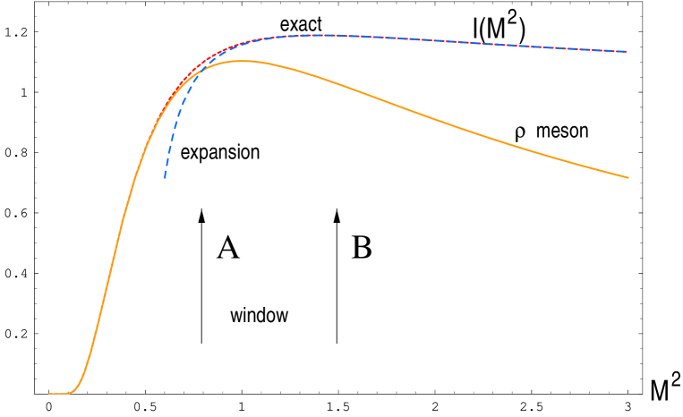
Figure 6: The sum rule for the $\rho$ meson in the toy model.

To get an idea of the accuracy one can expect from the sum rule calculations of the $\rho$-meson parameters we must investigate how sensitive our results are to various assumptions regarding the spectral density. The spectral density presented in Fig. 4 is not fully realistic, for many reasons. If minor details affected the results too strongly, the SVZ method would be useless. The right edge of the window (arrow B) is chosen in such a way as to minimize the impact of the (unknown) details of the spectral density above the $\rho$-meson peak. Yet, it is important to obtain a quantitative measure of the corresponding uncertainty.

The most obvious unrealistic feature of the spectral density (10) is the infinitely narrow width of all resonances from the comb. It is true that in the multicolor QCD the width-to-mass ratio of all hadrons built from quarks is proportional to $1/N_{c}$ [10] and, thus, vanishes at $N_{c}\rightarrow\infty$. If $N_{c}$ is fixed, however, and we are interested in the widths of the excited states, there is another large parameter, the excitation number, which compensates for the effect of large $N_{c}$. Moving to the right along the $s$ axis in Fig. 4, very soon we find ourselves in the situation with the overlapping resonances – the $\delta$ functions in the comb representing the spectral density are smeared and the spectral density becomes perfectly smooth. Let us discuss the consequences of such dynamical smearing.

First of all, we must establish the dependence of the width $\Gamma_{n}$ on the excitation number $n$. If one believes that a string-like picture of color confinement develops in QCD, an asymptotic estimate of $\Gamma_{n}$ at large $n$ becomes a simple exercise. Unlike the $\rho$ meson and other low-lying classical states, for highly excited states the string-like picture of the chromoelectric tubes is expected to be fully relevant.

When a highly excited meson state is created by a local source, it can be considered, quasiclassically, as a pair of (almost free) ultrarelativistic quarks; each of them with energy $m_{n}/2$. These quarks are created at the origin, and then fly back-to-back, creating behind them a flux tube of the chromoelectric field. The length of the tube $L\sim m_{n}/\Lambda^{2}$ where $\Lambda^{2}$ represents the string tension. The decay probability is determined, to order $1/N_{c}$, by the probability of producing an extra quark-antiquark pair. Since the pair creation can happen anywhere inside the flux tube, it is natural to expect that

$$\Gamma_{n}\sim\frac{1}{N_{c}}L\Lambda^{2}=\frac{B}{N_{c}}m_{n}$$ (29)

where $B$ is a dimensionless coefficient of order one. I used here the fact that within the quasiclassical picture the meson mass $m_{n}\sim L\Lambda^{2}$. Thus, the width of the $n$-th excited state is proportional to its mass which, in turn, is proportional to $\sqrt{n}$ for the linear Regge trajectories .

This simple estimate was obtained in Ref. [13] long ago. Since the argument bears a very general nature, the square root dependence of $\Gamma_{n}$ should take place in all models with linear confinement. And it does, indeed! Recently, the square root formula for $\Gamma_{n}$ was obtained numerically [14] in the ’t Hooft model [15].

If Eq. (29) does indeed take place, it is not difficult to find the impact of the resonance widths on the spectral density. The infinitely narrow pole is substituted with

$$\frac{1}{Q^{2}+m_{n}^{2}}\,\rightarrow\,\frac{1}{Q^{2}+m_{n}^{2}-im_{n}\Gamma_{n}}\,\rightarrow\,\frac{1}{Q^{2}+m_{n}^{2}-im_{n}^{2}B/N_{c}}\,\rightarrow$$

$$\frac{1}{Q^{2}+m_{n}^{2}-\gamma Q^{2}\ln Q^{2}}\,\rightarrow\,\frac{1}{(Q^{2})^{1-\gamma}+m_{n}^{2}}\,,$$ (30)

where

$$\gamma=\frac{B}{\pi N_{c}}\,,$$ (31)

and I used the fact that $1/N_{c}$ is a small parameter. This explains the last transition in Eq. (30). For the same reason, in the third transition I replaced $m_{n}^{2}/N_{c}$ with $N_{c}^{-1}\pi^{-1}Q^{2}\ln Q^{2}$. Near the pole (i.e. at $Q^{2}=-m_{n}^{2}$) both expressions give the same in the leading $1/N_{c}$ approximation, and are equally legitimate .

As a result, all poles, which lied previously at positive real $q^{2}$, are now shifted onto unphysical sheets, away from the physical cut (Fig. 7). The $\delta$ functions in the spectral density are replaced by peaks with finite widths. Correspondingly, the toy model number two, which replaces Eq. (11) is

$$\Pi(Q^{2})=-\frac{N_{c}}{12\pi^{2}}\,\frac{1}{1-\gamma}\,\psi(z)+\,\mbox{Const.}\,,$$ (32)

where now $z$ is given by the following formula

$$z=\frac{(Q^{2})^{1-\gamma}+1}{3}\,.$$ (33)

The additional factor $(1-\gamma)^{-1}$ in the overall normalization is chosen to reproduce the free quark result (14) at large Euclidean $Q^{2}$. Note that the polarization operator defined by Eqs. (32) and (33) has the correct analytical structure: it is non-singular in the whole complex $Q^{2}$ plane, apart from the cut at real positive $q^{2}$. The singularities associated with the poles of the $\psi$ function lie on the unphysical sheet (Fig. 7).

Figure 7: Analytical structure of the polarization operator. ($a$) The polarization operator must be analytic everywhere in the complex $Q^{2}$ plane, except the cut running on the negative real semi-axis of $Q^{2}$ (positive real semi-axis of $q^{2}$). The imaginary part of the polarization operator must be positive at the upper side of the $q^{2}$ cut; ($b$) The mapping of the $Q^{2}$ plane onto the $z$ plane, Eq. (33). The physical sheet on the $Q^{2}$ plane corresponds to the $z$ plane with the shaded sector removed. The boundaries of the sector correspond to the lower and upper sides of the $q^{2}$ cut. The angle of the removed sector is proportional to $\gamma$.

The spectral density (i.e. the imaginary part of $\Pi$ at $q^{2}=s+i\epsilon$) takes the form of the sum of (modified) Breit-Wigner peaks

$$\rho(s)=\frac{3}{\pi(1-\gamma)}\sum_{k=0}^{\infty}\frac{s^{1-\gamma}\sin\pi\gamma}{[s^{1-\gamma}\cos\pi\gamma-(1+3k)]^{2}+[s^{1-\gamma}\sin\pi\gamma]^{2}}\,.$$ (34)

It is depicted in Fig. 8 for $B=0.6$ and $N_{c}=3$. Although the choice of the parameter $B$ is rather arbitrary, it is not unreasonable; it corresponds to $\Gamma/m\approx 0.2$. Experimentally the $\rho$ meson has a close width-to-mass ratio.

We can see on the picture a pronounced $\rho$-meson peak, accompanied by a deep dip, and then an almost smooth curve which approaches the asymptotic value (unity) in an oscillating mode. The smearing of the $\delta$ functions into a smooth curve occurs because the width of the excited states is proportional to $m_{n}$ while the distance between two neighboring states $\Delta m_{n}\sim 1/m_{n}$. It is assumed, of course, that $N_{c}$ is fixed. The larger the value of $N_{c}$, the further we must go, to higher excitation numbers, for the resonances to overlap. Figure 8 shows that at $N_{c}=3$ a smooth curve starts right after the ground state. The first excitation already belongs to the smooth curve. Remember this pattern of the spectral density – a conspicuous first peak accompanied by a smooth (and oscillating) curve approaching its constant asymptotic value. The gross features of this picture follow from very general theoretical arguments [16]. We will see shortly that experimental data, being different in fine details, exhibits the very same type of behavior.

Figure 8: The spectral density corresponding to a sum of (modified) Break-Wigner peaks with one and the same width-to-mass ratio 0.2. All residues are set equal, and $\gamma\approx 0.06369$, see Eq. (34). The $s$ axis is in the units $m_{\rho}^{2}$.

The spectral densities shown in Figs. 4 and 8 at first sight do not produce an impression of close relatives. Let us integrate them over, with the exponential weight function, and compare $I(M^{2})$ obtained in this way. The comparison is shown in Fig. 9. The dotted curve corresponds to the comb of $\delta$ functions. It was already presented in Fig. 6. The solid curve corresponds to Eq. (34) and Fig. 8. Finally, the dashed curve is obtained with an extremely crude model of the spectral density depicted in Fig. 10,

$$\rho(s)=3\delta(s-1)+\theta(s-s_{0})\,,\,\,\,s_{0}=2.7\,.$$ (35)

It presents an infinitely narrow $\rho$, plus a gap, plus all higher excitations fused into “continuum” which starts abruptly at $s=s_{0}$ and coincides (at $s>s_{0}$) with the asymptotic free-quark expression for the spectral density. This is the original SVZ model [1]. It, obviously, captures only gross features, and misses all details: the fact that the gap at $s>m_{\rho}^{2}$ is not quite empty, the onset of continuum is not so abrupt, and the limit $\rho(s)\rightarrow 1$ at $s\rightarrow\infty$ is achieved through oscillations. Nevertheless, it is seen that $I(M^{2})$ in all three models come out very close to each other. The Breit-Wigner model of Eq. (34) gives a little bit less steep fall off to the left of the window, at $M^{2}\rightarrow 0$. This is quite understandable, since in this model there is a non-vanishing spectral density at $s<m_{\rho}^{2}$, due to the $\rho$ meson width.

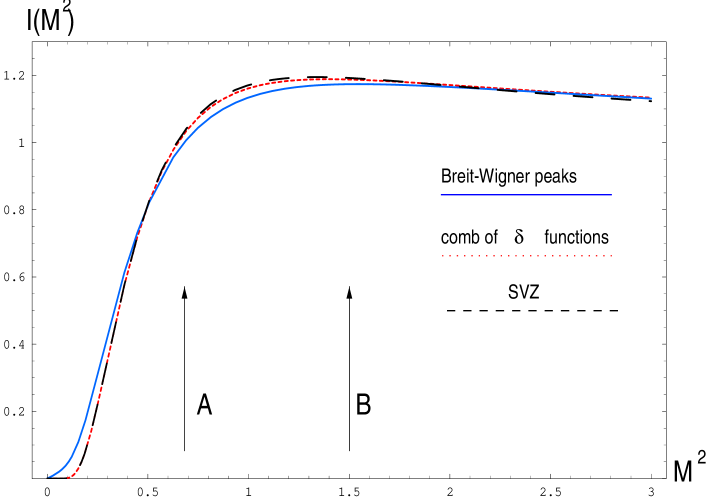
Figure 9: $I(M^{2})$ for three models of the spectral density.

Figure 10: The original SVZ model of the spectral density.

Comparison of three curves in Fig. 9 teaches us a lesson: by examining $I(M^{2})$, calculated approximately inside the window, one cannot expect to predict, with any reasonable accuracy, such fine structure of the spectral density as the width of the $\rho$ meson, and the shape of the curve in the continuum (i.e. higher excitations). As Fig. 9 shows, it is hardly possible to distinguish between three models under discussion, which, in a sense, represent extreme situations. The best one can hope for is estimating $m_{\rho}^{2}$, its residue, and, to a lesser extent, an effective value of $s$ where the dip following the $\rho$-meson peak ends (i.e. $s_{0}$).

In a broader context, this message is instructive for the lattice practitioners too. Doing calculations in the Euclidean domain – a common feature of the sum rules and lattice technology – derives virtually no information about the spectral density beyond the ground state in the given channel. Indeed, the original SVZ model and the comb of the $\delta$ functions, representing drastically different $\rho(s)$ point-by-point, lead to $I(M^{2})$ coinciding with each other to a high accuracy. To distinguish between these two scenarios one needs exponential precision going far beyond the level so far achieved in the lattice calculations.

Now we are ready to explore the sensitivity of $I(M^{2})$ to the $\rho$-meson parameters. To this end we will take the SVZ model in the form

$$\rho(s)=C_{1}\delta(s-C_{2})+\theta(s-s_{0})$$ (36)

and let the parameters float by, say, 10% around their “reference” values, $C_{1}=3,\,\,C_{2}=1$ and $s_{0}=2.7$. We then compare $I(M^{2})$ obtained in this way with $I(M^{2})$ emerging in our (most realistic) Breit-Wigner toy model, see Eq. (34).

Figure 11 illustrates the sensitivity of the sum rule to the $\rho$ meson residue (coupling constant). The upper and lower dashed curves correspond to $C_{1}=3.3$ and 2.7, respectively. Figure 12 illustrates the sensitivity to the $\rho$ meson mass. The upper and lower dashed curves correspond to $m_{\rho}^{2}=0.9$ and $1.1$ of the experimental value, respectively. It is seen that it is quite realistic to expect to get $g_{\rho}^{2}$ and $M_{\rho}^{2}$ with the accuracy $\sim 10\%$ by inspecting $I(M^{2})$ in the window and fitting the theoretical prediction by the model (36). The estimates of $s_{0}$ are less accurate. One should not be surprised, of course, since the sum rules were designed to be most sensitive to the ground-state parameters and relatively insensitive to the details of the spectral density in the continuum. The exponential weight in the definition of $I(M^{2})$ takes care of this feature. Deviations of $s_{0}$ from its reference value at the level of 10% lead to rather insignificant changes in $I(M^{2})$. Deviations of $s_{0}$ at the level of 20% are quite noticeable.

I hasten to add, however, that the 10% accuracy is not a typical outcome of the sum rule analysis. The $\rho$-meson channel is most favorable from the point of view of applications of the SVZ sum rules. In a sense, this is a dream case: the role of continuum with respect to $\rho$ is as tempered as it can possibly be, and higher (unknown) condensates in the truncated condensate expansion show up at remarkably low values of $M^{2}$ so that the working window is comfortably wide. In many other channels, mesonic and baryonic, we have to deal with a narrower window. The general rule is: the narrower the window the worse the accuracy. In some channels, as we will see later, the window shrinks to zero. Then the SVZ method fails. The reasons why it is successful in some cases and fails in others, when properly understood, give us a unique hint as to the structure of the QCD vacuum (see Sect. 8).

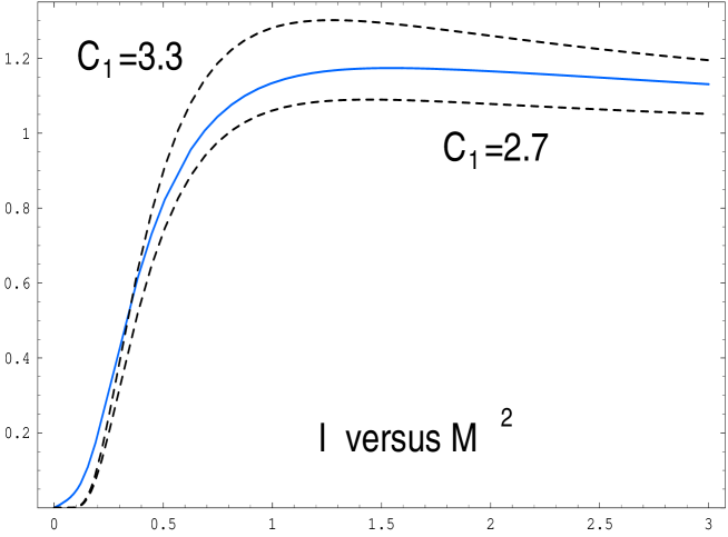
Figure 11: Changing the $\rho$ meson residue. The solid curve corresponds to a “reference” spectral density presented in Eq. (34). The dashed curves correspond to Eq. (36) with $C_{1}=3.3$ and 2.7, respectively. The reference value is $C_{1}=3$.

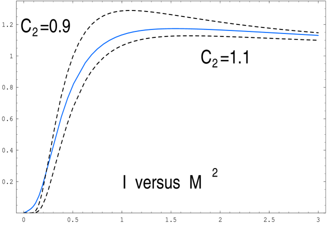
Figure 12: Changing the $\rho$ meson mass. The dashed curves correspond to the 10% variation of $m_{\rho}^{2}$, around its reference value ($m_{\rho}^{2}=1)$.

3 Vacuum Condensates

It is high time to abandon our baby version of QCD and proceed to the real thing. What can be said about $I(M^{2})$ now?

Needless to say that no analytic calculation of $I(M^{2})$ at $M^{2}\lower 3.01385pt\hbox{$\;\stackrel{{\scriptstyle\textstyle<}}{{\sim}}\;$}\Lambda^{2}$, that would be based entirely on the first principles, exists. QCD at large distances is not yet solved analytically. Under the circumstances it seems reasonable to start at short distances and advance to larger distances “step by step”, staying on the solid ground – working with the microscopic variables, quarks and gluons, where it is fully legitimate. At short distances the quark-gluon interactions are adequately described by perturbation theory. Certainly, as we have just learned by inspecting the toy models, the (truncated) perturbative series is not going to yield us any estimates relevant to the $\rho$ meson parameters. To get them we should add at least some information regarding the large distance dynamics.

In the ideal world this information would be obtained from the theory per se. In the real world we may try to parametrize the effects caused by the vacuum fields. If the quark-antiquark pair injected in the vacuum by the current $J_{\mu}$ does not propagate too far, its impact on the vacuum fields is, hopefully, not drastic. This means that the polarization operator can be well approximated by the interaction of the valence quarks with a few vacuum condensates. For the validity of this assumption it is necessary that the characteristic frequencies of the valence quarks inside the $\rho$ meson $\omega$ be larger than the characteristic scale parameter of the vacuum medium $\mu$. Certainly, we can count only on an interplay of numbers: since the only dimensional parameter of QCD is $\Lambda$, all quantities of dimension of mass are of order $\Lambda$. It may well happen, however, that, say $\omega\sim 3\Lambda$ while $\mu\sim\Lambda/2$. In a sense, the success of the SVZ sum rules confirms this assumption a posteriori.

On general grounds it is expected that all gauge invariant Lorentz singlet local operators built of the quark and/or gluon fields develop non-vanishing vacuum expectation values (VEV’s). It is convenient to order all operators (and their VEV’s) according to their normal dimensions. The higher the dimension, the higher the power of $1/M$ of the corresponding coefficient. This fact allows one to control the condensate expansion inside the working window.

The lowest dimension (zero) belongs to the unit operator. The unit operator is trivial. When one calculates the perturbative contribution to $I(M^{2})$, one actually calculates the coefficient of the unit operator.

The operator of the next lowest dimension (three) is the quark density operator,

$${\cal O}_{q}=\bar{q}q\,.$$ (37)

No other gauge and Lorentz invariant operators of dimension three exist.

There is one operator of dimension four, the gluon operator

$${\cal O}_{G}=\frac{\alpha_{s}}{\pi}G_{\mu\nu}^{a}G_{\mu\nu}^{a}\,.$$ (38)

The factor $\alpha_{s}/\pi$ appears in the definition naturally. Since both operators, (37) and (38), play a very special role we will interrupt our excursion before passing to higher dimensions, to make several important remarks.

In the chiral limit (i.e. when the quark mass term in the Lagrangian is put to zero) ${\cal O}_{q}$ is the order parameter – its VEV signals the spontaneous breaking of the axial $SU(N_{f})$ symmetry and the occurrence of the corresponding massless pions. In perturbation theory the chiral symmetry remains unbroken, of course, $\langle{\cal O}_{q}\rangle$ vanishes identically. It is tempting to say then that $\langle{\cal O}_{q}\rangle\neq 0$ measures deviations from perturbation theory, and the same refers to all other condensates.

In the early days of non-perturbative QCD such an understanding was widely spread. I hasten to say that this is a wrong understanding. It is impossible to define the condensates as “truly non-perturbative” residues obtained after subtracting from them a “perturbative part” [17]. A heated debate took place in the literature in the eighties regarding the possibility of defining the condensates, in a rigorous way, by subtracting a “perturbative part”. Glimpses of the debate can be seen in Ref. [18] where it was clearly emphasized, for the first time, that the procedure of isolating “purely non-perturbative” quantities does not (and must not) work . I will outline the proper procedure below using the gluon condensate as the most instructive example.

Unlike ${\cal O}_{q}$, the gluon operator ${\cal O}_{G}$ is not an order parameter. There is no known symmetry whose spontaneous breaking would generate a vacuum expectation value $\langle{\cal O}_{G}\rangle$. Correspondingly, $\langle{\cal O}_{G}\rangle$ is generated in perturbation theory. Physically, $\langle{\cal O}_{G}\rangle$ measures the vacuum energy density $\varepsilon_{\rm vac}$. To see that this is indeed the case let us use the fact that the trace of the energy-momentum tensor

$$\theta_{\mu}^{\mu}=-\frac{b}{8}\,\frac{\alpha_{s}}{\pi}G_{\mu\nu}^{a}G_{\mu\nu}^{a}\,.$$ (39)

This expression is nothing but the scale anomaly of QCD [20]. Strictly speaking, the coefficient on the right-hand side contains higher orders in $\alpha_{s}$; they are not essential for our purposes, however, and will be ignored. The vacuum expectation value of the left-hand side is obviously $4\varepsilon_{\rm vac}$. Hence

$$\varepsilon_{\rm vac}=-\frac{b}{32}\,\langle{\cal O}_{G}\rangle\,.$$ (40)

Everybody knows that the vacuum energy density badly diverges in field theory, as the fourth power of the cut-off . If so, how can one make sense of the gluon condensate?

The vacuum fields fluctuate; these fluctuations contribute to the vacuum energy density. High frequency modes of the fluctuating fields belong to the weak coupling regime; their contribution in the correlation functions is described by perturbation theory, giving rise to the standard perturbative expansions. What we are interested in are the low frequency modes, soft vacuum fields that are responsible for the peculiar properties of the vacuum medium. By saturating the condensate by the soft modes only we get a consistent definition of the condensates that automatically solves the problem of divergencies.

Specifically, we must introduce a somewhat artificial boundary, $\mu$: all fluctuations with frequencies higher than $\mu$ are supposed to be hard, those with frequencies lower than $\mu$ soft. The parameter $\mu$ is usually referred to as normalization point. Only soft modes are to be retained in the condensates. Thus, the separation principle is “soft versus hard” rather than “perturbative versus non-perturbative”. This is the basic principle of Wilson’s operator product expansion, which, in turn, is the foundation of the SVZ sum rules. Being defined in this way the condensates are explicitly $\mu$ dependent. All physical quantities are certainly $\mu$ independent; the normalization point dependence of the condensates is compensated by that of the coefficient functions.

Generalities of Wilson’s approach and its particular implementation in QCD will be further discussed in Sects. 5 and 6. Here we complete our consideration of the gluon condensate.

It is instructive to trace how the gluon condensate emerges from a slightly different perspective. A natural starting point is the diagram of Fig. 13 presenting the one-gluon correction to $\Pi(Q^{2})$ (two other similar graphs with the one-gluon exchange are not shown). For convenience we will deal with the so called $D$ function,

$$D(Q^{2})=-(4\pi^{2})Q^{2}(d\Pi/dQ^{2})\,,$$ (41)

rather than with the polarization operator $\Pi$ itself. In terms of $D(Q^{2})$ the bare quark loop of Fig. 5 becomes just unity.

Figure 13: The one-gluon correction to the $D$ function.

If the gluon momentum is denoted by $k$ the one-gluon term in $D(Q^{2})$ takes the form

$$\Delta D(Q^{2})=\alpha_{s}\int k^{2}dk^{2}\,\frac{1}{k^{2}}\,F(k^{2},Q^{2})$$ (42)

where it is implied that the angular integration over the orientations of the vector $k$ with respect to $q$ is already carried out. The factor $1/k^{2}$ comes from the gluon propagator, while $F(k^{2},Q^{2})$ represents the rest of the graph. The function $F(k^{2},Q^{2})$ was calculated in Ref. [21] (it can also be extracted from Appendix B of Ref. [22]),

$$F(k^{2},Q^{2})=\frac{8}{3\pi}\frac{1}{Q^{2}}\,\left\{\left(\frac{7}{4}-\ln\tau\right)\tau+(1+\tau)\left[L_{2}(-\tau)+\ln\tau\ln(1+\tau)\right]\right\}\,,$$ (43)

where

$$\tau=\frac{k^{2}}{Q^{2}}\,,$$

and

$$L_{2}(x)=-\int_{0}^{x}dyy^{-1}\ln(1-y)$$

is the dilogarithm function. The analytic continuation of the function (43) to $\tau>1$ can be more conveniently rewritten as

$$F(k^{2},Q^{2})=\frac{8}{3\pi}\frac{1}{Q^{2}}\,\left\{1+\ln\tau+\left(\frac{3}{4}+\frac{1}{2}\ln\tau\right)\frac{1}{\tau}\right.+$$

$$\left.(1+\tau)\left[L_{2}(-1/\tau)-\ln\tau\ln(1+\tau^{-1})\right]\right\}\,.$$ (44)

Substituting Eqs. (43) and (44) in Eq. (42) and doing the integral over $k^{2}$ in the most straightforward manner one gets $\Delta D=\alpha_{s}/\pi$, the standard well-known one-gluon correction to the $D$ function.

The plot of the function $F(k^{2},Q^{2})$ is shown in Fig. 14. Although it has a clear-cut peak at $\tau\sim 0.5$, it presents a distribution spanning the entire range from $k^{2}=0$ to $k^{2}=\infty$. The gauge coupling constant $\alpha_{s}$ in Eq. (42) is literally a constant provided one limits oneself to the graph of Fig. 13. In higher orders, however, $\alpha_{s}$ starts running, and it is evident that $\alpha_{s}\rightarrow\alpha_{s}(k^{2})$. Then $\alpha_{s}(k^{2})$ should be placed inside the integral in Eq. (42) rather than outside. By doing so we effectively resum a subset of the multi-gluon graphs.

Figure 14: The distribution function $Q^{2}F(k^{2},Q^{2})$ defined in Eq. (42) versus $\tau$.

Certainly, putting

$$\alpha_{s}(k^{2})=\alpha_{s}(Q^{2})\left[1+\frac{b\alpha_{s}(Q^{2})}{4\pi}\,\ln\frac{k^{2}}{Q^{2}}\right]^{-1}$$ (45)

inside the integral in Eq. (42) we do not account for all higher-order corrections. Only those are included that are responsible for the running of $\alpha_{s}$ in the leading logarithmic approximation. Usually they say that the corresponding multigluon graphs are of the bubble chain type (Fig. 15). Strictly speaking, in the covariant gauges the gauge coupling renormalization (45) in QCD (unlike QED) does not reduce to the bubble insertions in the gluon propagator depicted in Fig. 15. Various graphs of a more complicated structure are involved too; they combine together to produce a gauge-invariant expression (45). The bubble chain saturation of Eq. (45) takes place in the physical gauges, e.g. in the Coulomb gauge. In the covariant gauges one can artificially reduce the problem to the bubble chains, without explicit identification of the full set of graphs, by exploiting the so called “large negative $N_{f}$ trick”. We will not dwell on this technical issue, since it is irrelevant for our purposes. The interested reader is referred to Refs. [21, 22].

Even though the bubble chain is a very specific subset of graphs, and the majority of the multigluon graphs are left aside in this procedure, it still makes sense to substitute the running $\alpha_{s}(k^{2})$ inside the integral in Eq. (42), since in this way we take into account an essential part of the underlying dynamics: the fact that the quark-gluon interaction becomes weak if the gluon is far off-shell, and, on the contrary, becomes stronger as the gluon virtuality decreases. If we follow this strategy, then

$$\Delta D(Q^{2})=\int_{0}^{\infty}\alpha_{s}(k^{2})dk^{2}\,F(k^{2},Q^{2})=$$

$$\alpha_{s}(Q^{2})\int_{0}^{\infty}dk^{2}\left[1+\frac{b\alpha_{s}(Q^{2})}{4\pi}\,\ln\frac{k^{2}}{Q^{2}}\right]^{-1}\,F(k^{2},Q^{2})\,.$$ (46)

We immediately run into a problem here. The running $\alpha_{s}$ has the Landau pole at small $k^{2}$, the square bracket in the integrand explodes right inside the integration interval. The explosion occurs at

$$k^{2}=Q^{2}\exp\left[-\frac{4\pi}{b\alpha_{s}(Q^{2})}\right]=\Lambda^{2}\,.$$ (47)

Although the function $F(k^{2},Q^{2})$ is suppressed at small $k^{2}$, i.e. $\tau\rightarrow 0$, (see Fig. 14), it by no means vanishes at $\tau=\Lambda^{2}/Q^{2}$, rendering the integration impossible. In order to do the $k^{2}$ integral literally, as it is given in Eq. (46), we must say how the singularity at $k^{2}=\Lambda^{2}$ is to be treated. Some people say: “let us take the principal value”, others bypass the singularity by shifting the integration contour in the complex $k^{2}$ plane, still others do something else. All these prescriptions are arbitrary and physically meaningless for obvious reasons. Indeed, let us introduce the normalization point $\mu=$ several units $\times\Lambda$ and split the integration over $k^{2}$ in two parts: from zero to $\mu^{2}$ in the first integral and from $\mu^{2}$ to $\infty$ in the second. Then at $k^{2}>\mu^{2}$, in the weak coupling domain, we do trust Eq. (46) while below $\mu^{2}$ we do not. At best, below $\mu^{2}$ one can use Eq. (46) for the purpose of orientation. At small $k^{2}$

$$F(k^{2},Q^{2})\rightarrow\frac{2}{\pi}\,\frac{k^{2}}{Q^{4}}\,,$$ (48)

implying that

$$\Delta_{\{k^{2}<\mu^{2}\}}D(Q^{2})=\frac{2\alpha_{s}(Q^{2})}{\pi}\,\frac{1}{Q^{4}}\,\int_{0}^{\mu^{2}}k^{2}dk^{2}\left[1+\frac{b\alpha_{s}(Q^{2})}{4\pi}\,\ln\frac{k^{2}}{Q^{2}}\right]^{-1}\sim$$

$$\frac{8}{b}\,\,\frac{1}{Q^{4}}\,\int_{0}^{\mu^{2}}k^{2}dk^{2}\,\frac{\Lambda^{2}}{k^{2}-\Lambda^{2}}\,\sim\,\frac{8\pi}{b}\,\frac{\Lambda^{4}}{Q^{4}}\,.$$ (49)

This is a very crude estimate; I substituted the square bracket by the corresponding pole, and then evaluated the integral by equating it to its imaginary part, i.e. substituting $(k^{2}-\Lambda^{2})^{-1}\rightarrow\pi\delta(k^{2}-\Lambda^{2})$.

Figure 15: One of the graphs from the bubble chain set.

From this exercise we learn the following lesson. The domain $k^{2}<\mu^{2}$ gives a contribution to $D(Q^{2})$ which scales as $1/Q^{4}$. The coefficient in front of $1/Q^{4}$ cannot be reliably calculated and must be parametrized by the gluon condensate – that is the best we can do. It is not accidental that the $k^{2}$ expansion of $F(k^{2},Q^{2})$ starts from $k^{2}$, while the term of the zero-th order is absent. If it were not the case, the condensate series would have to start from ${\cal O}(Q^{-2})$. This is impossible, however, since no gauge invariant local operator of dimension two exists in QCD. The absence of such operator and the absence of terms $k^{0}$ in the distribution function $F(k^{2},Q^{2})$ are in one-to-one correspondence.

At first sight, one could try to circumvent the problem of the Landau pole inside the integration domain by expanding the square bracket in Eq. (46) in the series in $\alpha_{s}(Q^{2})$. This is one of the “remedies” sometimes cited in this context. I put the word remedy in the quotation marks since in fact it does not work. True, in every given order of the $\alpha_{s}$ expansion the integral (46) becomes well-defined. It is easy to see, however, that the expansion is going to be factorially divergent in high orders. Indeed,

$$\int_{0}^{\mu^{2}}k^{2}dk^{2}\left(\ln\frac{Q^{2}}{k^{2}}\right)^{n}\sim 2^{-n}n!\,,\,\,\,n\gg\ln\frac{Q^{2}}{\mu^{2}}\,.$$ (50)

It is seen that perturbation theory per se carries the seeds of the gluon condensate. The perturbative series cannot be consistently defined unless the gluon condensate is introduced. Once we cut off the $k^{2}<\mu^{2}$ tail of the integral from the perturbative expression obtained from Eq. (46), the factorial divergence of the $\alpha_{s}$ series at high $n$ disappears, the series becomes well-defined, and so is the gluon condensate.

The factorial divergence of the perturbative series of the type we have just discussed is called the infrared renormalon [23, 24] for the reasons which need not concern us here. It is associated with the bubble chain graphs of Fig. 15 and is inevitable if one forces the perturbative integrals to run all the way down to $k^{2}=0$. Bounding the integration interval in the perturbative part from below by $\mu^{2}$ we get rid of the infrared renormalon altogether. The domain below $\mu^{2}$ is not lost; it is fully represented by the gluon condensates. Higher condensates appear as higher order terms in the $k^{2}$ expansion of $F(k^{2},Q^{2})$. The intimate relationship between the infrared renormalons and condensates was first revealed by Mueller [25].

I hasten to warn that one should not literally equate the infrared renormalons to the condensate expansion. Even if one sticks to a certain particular definition for summation of the bubble chains, that eliminates ambiguities, say the principal value prescription in the integral (46), one typically gets a numerical value of the $Q^{-4}$ term which is grossly off compared to the gluon condensate, let alone ambiguities associated with various possible choices of the regularization prescription. For instance, in the case at hand,

$$D(Q^{2})=1+\frac{2\pi^{2}}{3Q^{4}}\langle{\cal O}_{G}\rangle+...\,,$$ (51)

and the ${\cal O}(1/Q^{4})$ term is $0.08\,\,\mbox{GeV}^{4}/Q^{4}$ under the standard choice of the gluon condensate (see below). Equation (49) yields, on the other hand, only $0.004\,\,\mbox{GeV}^{4}/Q^{4}$ at $\Lambda=0.2$ GeV ($0.01\,\,\mbox{GeV}^{4}/Q^{4}$ at $\Lambda=0.25$ GeV). Within the SVZ method, based on Wilson’s expansion, the role of the infrared renormalons is purely illustrative. They show, in a very straightforward manner, that without the condensates the perturbative series cannot be defined and, on the contrary, introducing the condensates one eliminates ambiguities associated with the high-order tails of the perturbative series .

On the other hand, in some (perturbatively infrared stable) processes that have no operator product expansion, most notably in the jet physics, the infrared renormalons, in spite of all their obvious limitations, become poor man’s substitute for the condensate expansion. Although, unlike OPE, the renormalon analysis does not provide us with the proper numerical coefficients, we may infer from the renormalons what powers of $1/E$ (or $1/Q$) appear in the nonperturbative parts of such quantities as, say, thrust. Whether the nonperturbative corrections are ${\cal O}(1/E)$ or ${\cal O}(1/E^{2})$ is clearly a question of paramount importance for phenomenology. Using the infrared renormalons for counting the powers of $1/E$ in the processes without OPE is a totally fresh idea which can be considered as a distant spin off of the SVZ method, see Ref. [27] for a review. Previously the nonperturbative corrections were just ignored since nobody knew how to approach the issue scientifically.

Now, when the meaning of the condensates appearing in Wilson’s expansion is hopefully clear, we can proceed to a brief discussion of their numerical values. In principle, two alternative approaches are conceivable: (i) calculating the condensates from first principles (e.g. on the lattices); (ii) extracting the condensates from the sum rules themselves. Attempts of the lattice calculation of the condensates were reported in the literature (for a review see [28]). The main difficulty, which, to a large extent, devaluates this work is the fact that the strategy of “isolating a non-perturbative residue from the perturbative background” was adopted. As we already know, this strategy is doomed to failure. Instead, one should have consistently implemented Wilson’s procedure. This has never been done, however. Some initial ideas as to how Wilson’s procedure can be implemented on the lattices are presented in Ref. [29].

Therefore at present, as twenty years ago, one has to exploit the sum rule themselves in order to determine the condensates. One picks up certain channels where sufficient experimental information on the corresponding spectral densities is available. These channels are sacrificed, i.e. the analysis goes in the direction opposite to conventional: the values of the condensates are extracted from the Euclidean correlation functions obtained through dispersion integrals. The first determination of the gluon condensate was carried out exactly in this way, from the sum rules in the $J/\psi$ channel [30, 1]. The corresponding value will be referred to as standard,

$$\langle{\cal O}_{G}\rangle=0.012\,\,\mbox{GeV}^{4}\,.$$

Since then this estimate was subject to multiple tests, sometimes with conflicting results. A brief discussion can be found in the beginning of Sect. 2 in Ref. [2]. The overall conclusion is that certain deviations from the standard value (say, at the level of $\sim 30\%$) are not ruled out . One of the reasons limiting the accuracy is the fact that the gluon condensate was determined within a simplified (the so called practical) version of the operator product expansion, which is strictly speaking somewhat ambiguous. We will dwell on the issue in Sect. 6. At the present level of understanding it is highly desirable to repeat the analysis within the framework of consistent Wilson’s procedure. This is not done so far. To take into account a certain degree of numerical uncertainty it is reasonable to accept that

$$\langle{\cal O}_{G}\rangle=0.012\,x_{G}\,\,\,\mbox{GeV}^{4}\,,$$ (52)

where a dimensionless numerical factor $x_{G}$ is allowed to float in the vicinity of unity. This parametrization will be used below in the $\rho$-meson sum rule.

Let us pass now to the quark condensate $\langle{\cal O}_{q}\rangle$. As was mentioned, this condensate is the order parameter for the spontaneous breaking of the chiral symmetry. Hence, its value can be independently determined from the corresponding phenomenology. In particular, the celebrated Gell-Mann–Oakes–Renner formula relates the product of the light quark masses and $\langle{\cal O}_{q}\rangle$ to observable quantities,

$$(m_{u}+m_{d})\langle\bar{u}u+\bar{d}d\rangle=-M_{\pi}^{2}f_{\pi}^{2}\,,$$ (53)

where $f_{\pi}$ is the pion constant ($f_{\pi}\approx 133$ MeV) and $M_{\pi}$ is the pion mass. The original estimate of $\langle{\cal O}_{q}\rangle$ used in Ref. [1] was obtained by substituting the crude estimates of the light quark masses that existed at that time [31, 32],

$$m_{u}+m_{d}\approx 11\,\,\mbox{MeV}\,.$$

In this way one arrives at

$$\langle{\cal O}_{q}\rangle=-(250\,\,\mbox{MeV})^{3}\,.$$ (54)

Since then considerable work has been carried out to narrow down the theoretical uncertainty. First of all, chiral corrections to the Gell-Mann–Oakes–Renner formula were derived and analyzed. Moreover, much effort has been invested in perfecting our knowledge of the quark masses. The progress is summarized in Ref. [33], where an extensive list of references can be found. No dramatic changes occurred. The value of $m_{u}+m_{d}$ extracted from phenomenology of the chiral symmetry breaking went up by about 30%, with an error at the level of 15%. Thus, one is tempted to say that the actual value of the quark condensate is close to its “standard” value quoted in Eq. (54); perhaps, somewhat suppressed .

Events took a dramatic turn in 1996, after results of the lattice calculations of the light quark masses (with two dynamical quarks) became known. The lattice result for $m_{u}+m_{d}$ lies significantly lower (by a factor of two to three, see e.g. [34]) than any of the reasonable analytic estimates! Were these results confirmed, this would mean that the quark condensate is significantly larger than the number given in Eq. (54).

I would caution against hasty conclusions at this point. The discrepancy between the analytic and lattice estimates may well be an artifact of the lattice procedure. Putting dynamical almost massless quarks on the lattice is a notoriously difficult task. On the other hand, the discrepancy, if persists, may prove to be a signature of a very interesting physical phenomenon – strong dependence of physical quantities on the number of light dynamical quarks. The surprisingly low lattice result for $m_{u}+m_{d}$ was obtained under the assumption that the number of light quarks is two, while in fact it is three. We will return to the issue of possible strong dependence on $N_{f}$ in Sect. 12.

Under the circumstances it seems reasonable, analogously to the gluon condensate, to parametrize the quark condensate as

$$\langle{\cal O}_{q}\rangle=-(250\,\,\mbox{MeV})^{3}\,x_{q}\,,$$ (55)

and let $x_{q}$ vary around unity.

The full catalog of all relevant operators up to dimension six, was worked out in Ref. [1]. It is not as large as one might think at first sight. There is only one operator of dimension five, the mixed quark-gluon operator

$${\cal O}_{qG}={ig}\,\bar{q}\sigma_{\mu\nu}G_{\mu\nu}q$$ (56)

where $G_{\mu\nu}\equiv G_{\mu\nu}^{a}T^{a}$ ($T^{a}$ are the color generators). This operator plays no role in the $\rho$-meson sum rules, to be considered below: because of its “wrong” chirality it can enter only being multiplied by the quark mass $m_{q}$. It is very important, however, in a wide range of problems involving baryons [35], and mesons built from one light and one heavy quarks [36].

At the level of dimension six, there is one operator built from three gluon field strength tensors (symbolically $GGG$) and several four-quark operators of the type

$${\cal O}_{4q}=(\bar{q}_{1}\Gamma_{1}q_{2})(\bar{q}_{3}\Gamma_{2}q_{4})$$ (57)

where $\Gamma_{1,2}$ denote certain combinations of the Lorentz and color matrices and $q_{i}$ ($i=1,...,4$) are the light quark fields of different flavors, $u,d$ and $s$. The overall flavor must be conserved of course, but $q_{1}$ need not coincide with $q_{2}$ and so on.

The three-gluon operator is expected to have a significant impact in heavy quarkonium [37]; it does not appear in the $\rho$-meson sum rules, as was first shown in Ref. [38], by virtue of a very elegant theorem.

As for the four-quark operators, their vacuum matrix elements are not known independently. It became standard to evaluate them in the factorization approximation, which was first applied in this context in [1]. Note that using the Fierz identities for the color and Lorentz matrices one can always arrange the operators ${\cal O}_{4q}$ to have a natural color flow. By natural I mean that $\Gamma_{1,2}$ do not contain color matrices, and the color indices of quarks are contracted inside each bracket in Eq. (57). The color of $q_{1}$ flows to $q_{2}$ and that of $q_{3}$ flows to $q_{4}$. If the number of colors $N_{c}$ were large, then the expectation value of ${\cal O}_{4q}$ would be totally saturated by the vacuum intermediate state,

$$\langle{\cal O}_{4q}\rangle=\langle\bar{q}_{1}\Gamma_{1}q_{2}\rangle\langle\bar{q}_{3}\Gamma_{2}q_{4}\rangle\,.$$ (58)

Corrections to this equation are formally of order of $1/N_{c}^{2}$. It is clear that in the factorization approximation, after the natural color flow is achieved by the Fierz rearrangement, the only surviving structure is that with $\Gamma_{1,2}=1$.

In the real world $N_{c}=3$, and we certainly do expect deviations from factorization at a certain level. As far as we can tell today, factorization works surprisingly well at least for those four-quark operators that appear in the $\rho$-meson sum rule. All attempts to detect deviations, both on the lattices [39] and in the sum rules themselves [40], gave results consistent with zero, within errors that typically lie in the 10% ballpark. This is quite nontrivial, considering the fact that quite a few examples are known where large numerical coefficients neutralize formal $1/N_{c}$ suppression factors. Whatever the reasons might be, we will accept Eq. (58) in what follows.

4 $\rho$ Meson in QCD

Experience accumulated in Sect. 2 will now be applied for explorations in actual QCD. As we learned from the toy models, the polarization operator $\Pi(Q^{2})$ (or its Borel transform $\tilde{\Pi}(M^{2})$) in the deep Euclidean domain has an expansion in $\ln Q^{2}$ (perturbation theory) plus power terms $(1/Q^{2})^{k}$ or $(1/M^{2})^{k}$ (the condensates). If in the toy models the power terms (truncated in certain order) can be made as large or as small as we want, in QCD they are determined dynamically; through interactions of the valence quark pair with the soft vacuum fields. This interaction gives rise to the condensate expansion. The first power term is due to the gluon condensate, while the next one is associated with the four-quark condensate. In principle, higher condensates were analyzed in the literature too, but we will not discuss them in this Lecture.

The quark-antiquark pair $q\bar{q}$ with the total energy $\sqrt{s}$ is injected in the QCD vacuum either by the virtual photon ($e^{+}e^{-}$ annihilation) or $W$ boson ($\tau$ decays). The $q\bar{q}$ pair, being injected, starts evolving according to the dynamical laws of QCD. At first the quarks do not feel the impact of the vacuum “medium”. As separation between them grows, the effects of the medium become more and more important, so that eventually it prevents quarks from appearing in the detectors. The injected quarks get dressed and materialize themselves in the form of hadrons. In the sum rule approach we control only the beginning of this process.

In the sum rule framework, the condensates become important in the vicinity of the left edge of the window. To the left of the arrow $A$ they explode, and theoretical control is lost. On the other hand, the value of $I(M^{2})$ near the right edge of the window is determined mostly by ordinary perturbation theory. All perturbation theory sits in the unit operator. Technically it is convenient to formulate the corresponding calculation in terms of the perturbative corrections to the spectral density. We take the graph of Fig. 5, and attach to it various gluon and quark loops (e.g. Figs. 13 and 15). In this way we get the perturbative part of $\rho(s)$; at present in the vector isovector channel it is known up to third order in $\alpha_{s}(s)$ [41]. In the $\overline{\mbox{MS}}$ scheme the result takes the form

$$\rho(s)=1+k_{1}a+k_{2}a^{2}+k_{3}a^{3}$$ (59)

where $a(s)$ is given in Eq. (3). In the low-energy domain the number of active flavors is $N_{f}=3$. For $N_{f}=N_{c}=3$ the parameter $b=9$, and the values of $k_{i}$ are

$$k_{1}=\frac{4}{9}\,,\;\;\;k_{2}=0.729k_{1}\,,\;\;\;k_{3}=-2.03k_{1}\,.$$ (60)

Equation (59) can be immediately translated into the prediction for the perturbative part of $I(M^{2})$. The perturbative expansions for $I(M^{2})$ and $\rho(s)$ do not coincide. To get the former one must integrate the latter with the exponential weight function. The transition is readily carried out with the aid of the formula [42]

$$\int{ds\over M^{2}}\frac{\exp(-s/M^{2})}{\left(\ln\frac{s}{\Lambda^{2}}\right)^{\nu}}=\frac{1}{\left(\ln\frac{M^{2}}{\Lambda^{2}{\rm e}^{\gamma}}\right)^{\nu}}\left[1+\frac{\nu(\nu+1)}{2}\frac{\pi^{2}/6}{\left(\ln\frac{M^{2}}{\Lambda^{2}{\rm e}^{\gamma}}\right)^{2}}+{\cal O}\left(\frac{1}{\left(\ln\frac{M^{2}}{\Lambda^{2}{\rm e}^{\gamma}}\right)^{4}}\right)\right]\,,$$ (61)

where $\gamma$ denotes Euler’s constant, $\gamma=0.577$. Expanding this expression near integer values of $\nu$ one also gets necessary expressions for the integrals containing logarithm of logarithm ($\ln\ln$).

In this way we arrive at [42]

$$I_{\rm pc}(M^{2})=1+k_{1}a\left(\frac{M^{2}}{{\rm e}^{\gamma}}\right)+k_{2}\left[a\left(\frac{M^{2}}{{\rm e}^{\gamma}}\right)\right]^{2}+(k_{3}+\frac{\pi^{2}}{6}k_{1})\left[a\left(\frac{M^{2}}{{\rm e}^{\gamma}}\right)\right]^{3}\,.$$ (62)

Similar expressions were obtained in Ref. [43], were $a({M^{2}}/{{\rm e}^{\gamma}})$ was reexpressed in terms of $a(M^{2})$. It is more convenient to work directly with the expansion (62).

The quark mass corrections in $\rho(s)$ and $I(M^{2})$ are also known, they are proportional to $m_{u,d}^{2}/M^{2}$ and are negligibly small due to the smallness of the current quark masses. They will be discarded since the corresponding uncertainty is invisible in the background of other uncertainties.

Now we return to the condensates. The modern perturbative calculations of the coefficients $C_{n}$ are based on the background field technique. This is an important aspect of the SVZ approach as it exists today. The method is quite elegant, to say nothing that it is much more economic than the original “brute force” calculations of Ref. [1]. We will not discuss the technique per se, however. Conceptually everything is clear here. If you need to do a calculation, you just go and learn the corresponding technique using, for instance, the review paper [44].

The coefficients $C_{G}$ and $C_{4q}$, to the leading order, are known from the ancient times [1],

$$I_{\rm npc}(M^{2})=1+\frac{\pi^{2}}{3M^{4}}\,\langle{\cal O}_{G}\rangle-\frac{8\pi^{3}}{M^{6}}\,\left\langle\alpha_{s}\left(\bar{u}\gamma_{\alpha}\gamma_{5}T^{a}u-\bar{d}\gamma_{\alpha}\gamma_{5}T^{a}d\right)^{2}\right\rangle-$$

$$\frac{16\pi^{3}}{9M^{6}}\,\left\langle\alpha_{s}\left(\bar{u}\gamma_{\alpha}T^{a}u+\bar{d}\gamma_{\alpha}T^{a}d\right)\,\sum_{q}\left(\bar{q}\gamma_{\alpha}T^{a}q\right)\right\rangle\,.$$ (63)

The four-quark structures appearing in the angle brackets, as well as the factor $\alpha_{s}$ in front of them, are normalized at $Q$. The anomalous (logarithmic) dimension of this particular combination nearly vanishes [1]; we will ignore it in evolving the four-quark operator at hand down to $\mu$. Applying factorization, as was explained in Sect. 3, we get for the four-quark term in $I_{\rm npc}(M^{2})$

$$C_{4q}\langle{\cal O}_{4q}\rangle=-\frac{448\pi^{3}}{81M^{6}}\,\alpha_{s}(\mu)\langle\bar{q}q(\mu)\rangle^{2}\rightarrow-\frac{1}{M^{6}}\,0.03\,x_{4q}\,\,\mbox{GeV}^{6}\,,$$ (64)

where, as previously, we have introduced a factor $x_{4q}$ to allow for possible theoretical uncertainties. Under the standard choice of parameters [1] this factor is equal to unity. If we are on the right track it is reasonable to expect that $x_{4q}$ is close to unity.

A huge amount of work was carried out in calculating two-loop corrections in the coefficients of various condensates. The results can be inferred, say, from Ref. [45] or from the reviews [46]. Unfortunately, the existing uncertainty in the condensates themselves precludes us from taking advantage of the precision achieved in perturbative corrections. Therefore, we will limit ourselves to the leading order results for $C_{G}$ and $C_{4q}$.

Now, the stage is set and we can finally present the sum rule for $I(M^{2})$,

$$I(M^{2})=1+\frac{4}{9}\,a\left(\frac{M^{2}}{{\rm e}^{\gamma}}\right)\,\left\{1+0.729\,\left[a\left(\frac{M^{2}}{{\rm e}^{\gamma}}\right)\right]-0.386\,\left[a\left(\frac{M^{2}}{{\rm e}^{\gamma}}\right)\right]^{2}\,\right\}\,+$$

$$0.1x_{G}\left(\frac{0.6}{M^{2}}\right)^{2}-0.14x_{4q}\left(\frac{0.6}{M^{2}}\right)^{3}\,,$$ (65)

where $M$ in the second line of Eq. (65) is measured in GeV. The term $M^{-4}$ is due to the gluon condensate, while the term $M^{-6}$ is due to the quark condensate. With the “standard” numerical values of the gluon and quark condensates in the the nonperturbative part $x_{G}=x_{4q}=1$; the dimensionless constants $x_{G}$ and $x_{4q}$ allow the gluon and four-quark condensates to “breathe” to a certain degree. For instance, $x_{G}>1$ would imply that the actual value of the gluon condensate is larger than the “standard” value, and so on.

We are ready to examine the situation in the $\rho$-meson channel. Figure 16 shows experimental data on the spectral density in the vector isovector channel, measured in the $\tau$ decays. The data points are from Ref. [47]. Note a remarkably close resemblance with our toy model number two. If we take the beginning of Fig. 8 and expand it to make the energy scales coincide the curves will essentially repeat each other. There exist a few extra points in the $\tau$ decays, spanning the interval of $s$ from 2.7 to 3 GeV², and some data above 3 GeV² from the $e^{+}e^{-}$ annihilation, but the corresponding error bars are so large that plotting these points would just obscure the picture.

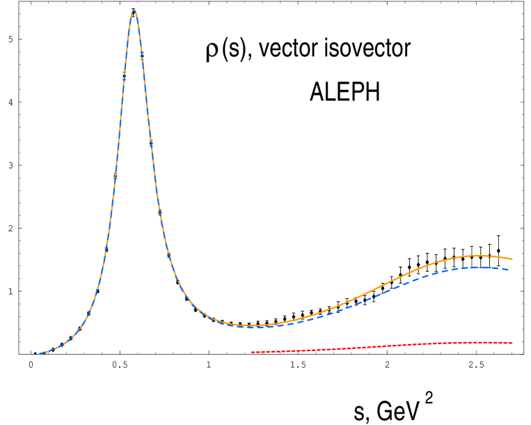
Figure 16: The spectral density in the vector isovector channel measured in $\tau$ decays. The data points belong to ALEPH. The solid curve is a best fit. The dashed curve is the best fit minus $KK\pi$ (the latter contribution is shown by the dotted curve) which, I think, should not have been included in the vector spectral density, see text.

There is a subtle point which I have to discuss here. Directly measurable in the hadronic $\tau$ decays is the sum of the vector and axial spectral densities. To obtain the spectral densities separately one has to sort out all decays by assigning specific quantum numbers to each given final hadronic state. In the majority of cases such an assignment is unambiguous. For instance, two pions (whose contribution is the largest) can be produced only by the vector current. Some processes, however, can occur in both channels, for instance, the $KK\pi$ production. Using certain theoretical arguments it was decided in Ref. [47] that around 3/4 of all $KK\pi$ yield should be ascribed to the vector channel. Other theoretical arguments [42], which seem to be much more convincing to me, tell that virtually all $KK\pi$ production should take place in the axial channel. Therefore, in dealing with the data, I will subtract the $KK\pi$ yield from the ALEPH data points. I hasten to add that the subtracted quantity is small (see Fig. 16), and this subtraction is not very essential for a general picture I draw here by broad touches.

The solid curve in Fig. 16 is a best fit by a smooth curve representing the sum of two Breit-Wigner peaks (the first one is a modified Breit-Wigner taking into account threshold effects important for the $\rho$ meson). The dashed curve is what I believe the actual spectral density is. The data points above 1 GeV² carry a noticeable uncertainty. Since we are going to use the spectral density only in the integrals, where many data points are summed over, these individual errors can be neglected, since they will be statistically insignificant in the integrals. Systematic uncertainty might be important, but since nobody knows how to estimate it, I will ignore it for the time being. For our limited purposes we can consider the dashed curve in Fig. 16 as an exact experimental result for the spectral density.

How does the experimental spectral density might look above 2.7 GeV²? This question is irrelevant for calculating the $\rho$-meson parameters. It is very instructive, however, to have a broader perspective. I will show you what I call a “theoretical experimental” spectral density, and then will make a short digression explaining where the answer comes from.

My expectations are summarized in Fig. 17. The curve to the left of the arrow is just the fit to the experimental data, as explained above (it identically coincides with the dashed curve in Fig. 16.) To the right of the arrow I have attached a “tail” which approaches a smooth asymptotic prediction for $\rho(s)$ (the dashed line) given in Eq. (59), in an oscillating manner. The tail and the experimental data are smoothly matched at 2.65 GeV².

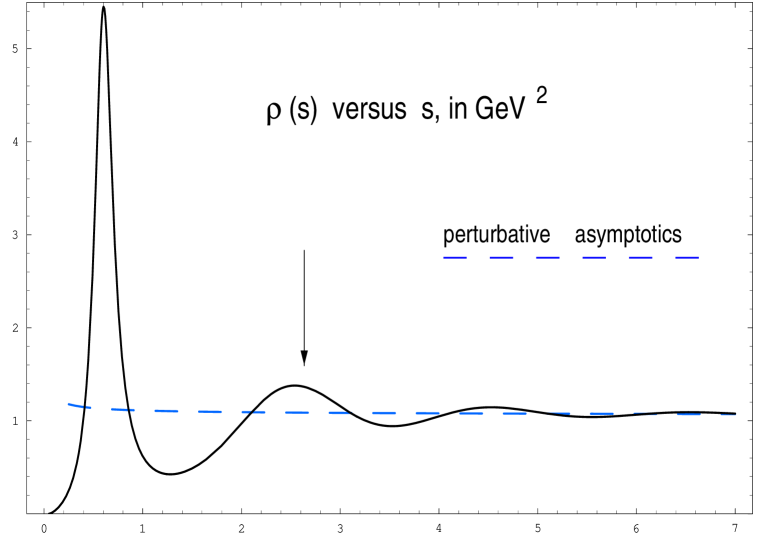
Figure 17: “Theoretical experimental” spectral density in the $\rho$ meson channel. The solid curve presents experiment (see text), while the dashed curve is the perturbative result for $\rho(s)$, including terms up to $O(\alpha_{s}^{3})$, with $\Lambda=0.2$ GeV.

Why I think that the actual spectral density, when and if it is measured, will approach the smooth asymptotic curve with oscillations rather than monotonously? The reason is of a very general nature [16]. In a nut shell, there are exponential terms that are not seen in the truncated OPE series for $\Pi(Q^{2})$ in the Euclidean domain. When these terms are analytically continued to the Minkowski domain, where Im $\Pi(s)$ belong, they show up as oscillating terms. The smooth asymptotic prediction is obtained from the truncated series and, thus, carries no traces of the exponential/oscillating terms. We will return to the issue later on (see Sect. 5).

Although the very existence of oscillations in the spectral densities may be considered firmly established, the question of how rapidly they die off is highly non-trivial and has no unambiguous answer in today’s theory. In resonance-inspired models the damping factor is $\sim\exp(-\mbox{const}\,s)$ (see Sect. 2.2), in the instanton-based models [48] it is $\sim\exp(-\mbox{const}\,\sqrt{s})$. The tail added in Fig. 17 is taken to be proportional to $\exp(-\pi\sqrt{s})\cos(\pi s+\mbox{const})$. This rather eclectic formula is chosen for sophisticated reasons which need not concern us here. The task which we address is illustrative, anyway. I certainly cannot guarantee that around 3.5 GeV² the value of $\rho(s)$ is 0.97, as it is shown in Fig. 17, but I could bet that a shortage of the spectral density in this domain will be observed in precision measurements, so that $\rho(s)$ at 3.5 GeV² will lie somewhere around unity. I emphasize again that the precise form of the tail does not affect the sum rule calculation of the $\rho$ meson parameters, and is discussed only for completeness of the picture.

With the experimental spectral density in hands, we can calculate the “experimental” value of the integral $I(M^{2})$. The corresponding result is presented in Fig. 18 by the solid curve.

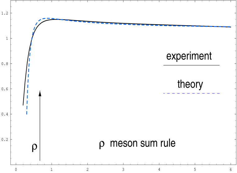
Figure 18: $I$ versus $M^{2}$ (in GeV²) in the $\rho$ meson channel: confronting experiment and theory. The theoretical curve corresponds to $x_{G}=0.8$, $x_{4q}=1.3$ and $\Lambda=0.2$ GeV.

The agreement is excellent; it is even better than one could expect apriori. We see that the conspicuous $\rho$ peak and all further twiddles characteristic to $\rho(s)$ are washed out. If we descend from larger to smaller values of $M$, the behavior of $I(M)$ is flat down to $M\sim 0.8$ GeV, i.e. down to the $\rho$ meson mass. At $M\sim 0.8$ GeV the regime smoothly changes, the curve dives down, and at still lower values of $M$, approaches the exponential asymptotics (this domain is not shown in the figure). The boundary value of $M$ where the regime changes is correlated with the mass of the lowest state, the $\rho$ meson in the case at hand. This is practically the only characteristic dimensional parameter in $I(M)$.

Let us pretend now that we do not know the spectral density and want to use the sum rules to determine the $\rho$ meson mass. It is quite clear that the truncated condensate series does not allow one to go to the limit $M\rightarrow 0$ where this determination would be exact: the series explodes. We must stay inside the window where the expansion is still under control. Correspondingly, our determination of $M_{\rho}$ is going to be approximate. The strategy can be formulated as follows. Let us assume that somebody shows us a sketch of the spectral density presented in Fig. 10 with the numbers along the horizontal and vertical axes erased. This sketch is known to correctly reproduce the basic features of the actual spectral density but leaves us ignorant as to where the $\rho$-meson peak lies and what is its height. We insert this sketch in our sum rule, do the integral

$$\frac{1}{\pi M^{2}}\,\int ds\,\rho(s)e^{-s/M^{2}}\,,$$

fit the numbers in such a way as to be as close to the theoretical prediction (65) inside the window – click, click – the scales are restored, and there come out the $\rho$ mass and the coupling constant. Since inside the window the $\rho$ meson saturates the integral at the level $\sim 90\%$ , the fact that our continuum model is a caricature (minor details are lost) is unimportant. Even if we are off by a factor of two in this model this will affect our estimates referring to the $\rho$ meson at the level of $\sim 10\%$.

This example is quite typical. A similar situation takes place for all classical low-lying hadrons: those built from the light quarks, heavy, and light and heavy. I do not define here precisely what the “classical meson” means but will return to this point later, after considering some nonclassical channels. I must admit that the $\rho$ meson is the example where the SVZ method demonstrates its best facets. The window is sufficiently broad, everything is clean. As we proceed to higher spins, the mesons become larger in size. A snapshot of a high-spin meson would show a string-like picture, with a longitudinal size of the “sausage” much larger than its transverse size. Under the circumstances one could hardly expect that the SVZ method would work. And, indeed, it ceases to be informative for spins higher than two [49].

5 Basic Theoretical Instrument – Wilson’s OPE

The theoretical basis of any calculation within the SVZ method is the operator product expansion (OPE). It allows one to consistently define and build the (truncated) condensate series for any amplitude of interest in the Euclidean domain. The physical picture lying behind OPE was described above: consistent separation of short and large distance contributions. The former are then represented by the vacuum condensates while the latter are accounted for in the coefficient functions. Thus, the operator product expansion in the form engineered by Wilson [50] is nothing but a book-keeping procedure. Wilson’s idea was adapted to the QCD environment in Ref. [18].

Although OPE is used in an innumerable amount of works since the mid-1970’s, there are no good text-books or reviews devoted to this issue. Moreover, one typically encounters a lot of confusion in the literature. Below I will try to explain the Wilsonean procedure using, as an example, the $T$ product of the two vector currents defined in Eq. (7).

Technically it is more convenient to deal with the $D$ function (41) rather than $\Pi_{\mu\nu}$,

$$D(q^{2})=\sum_{n}C_{n}(q;\mu)\langle{\cal O}_{n}(\mu)\rangle$$ (66)

where the normalization point $\mu$ is indicated explicitly. The sum in Eq. (66) runs over all possible Lorentz and gauge invariant local operators built from the gluon and quark fields. The operator of the lowest (zero) dimension is the unit operator I, followed by the gluon condensate $G_{\mu\nu}^{2}$, of dimension four. The four-quark condensate gives an example of dimension-six operators.

At short distances QCD is well approximated by perturbation theory. The coefficient functions $C_{n}$ absorb the short-distance contributions. Therefore, as a first approximation, it is reasonable to calculate them perturbatively, in the form of expansion in $\alpha_{s}(Q)\sim(\ln Q)^{-1}$. This certainly does not mean that the coefficients $C_{n}$ are free from non-perturbative, non-logarithmic terms of the type $\sim Q^{-\gamma}$ where $\gamma$ is a positive number.

To substantiate the point let us consider the coefficient of the unit operator. The Feynman graphs for $D(q^{2})$ of the lowest order are depicted in Figs. 5 and 13. Assume that the momentum flowing through the graph is Euclidean and large, $Q\rightarrow\infty$. If all subgraphs in these and similar graphs are renormalized at $Q$, the final result, being expressed in terms of the running coupling constant $\alpha_{s}(Q)$, is finite. The virtual momenta saturating the loop integrals scale with $Q$ as the first power of $Q$. At any finite order the perturbative series is well-defined.

At the same time, if the number of loops $n$ becomes very large, in a random graph (Fig. 19) each loop carries momentum of the same order of magnitude, and the total momentum $Q$ is shared between many lines, so that the characteristic virtual momentum is proportional to $Q/n$. The contribution of each graph to $C_{I}$ is of order $[\alpha_{s}(Q)]^{n}$, but the number of distinct diagrams $\nu$ grows factorially, $\nu\sim n!$, so that the expansion in $\alpha_{s}(Q)$ is asymptotic (for an exhaustive discussion of this phenomenon see Ref. [51]).

Figure 19: A typical multiloop graph contributing to the $D$ function. The number of such graphs grows factorially with the number of loops.

Note that this factorial divergence has nothing to do with the renormalon divergence considered in Sect. 3. There, we had one specific graph of the $n$-th order whose contribution was proportional to $n!$. This factorial was a spurious artifact of an improper calculation where the domain $k\sim\Lambda$ was included. Introducing a lower cut-off at $\mu$ = several units times $\Lambda$ and discarding the contribution coming from $k^{2}<\mu^{2}$, as it should be done in the consistent calculation of $C_{I}(\mu)$, we would eliminate the renormalon divergence. At the same time, the factor $n!$ counting the number of graphs of the $n$-th order certainly cannot be eliminated in this way.

If $n$ is not too large, so that $Q/n>\mu$, the graphs of Fig. 19 present a legitimate contribution to $C_{I}(\mu)$. It is quite clear that the tail of the $\alpha_{s}$ series with $n\lower 3.01385pt\hbox{$\;\stackrel{{\scriptstyle\textstyle>}}{{\sim}}\;$}1/\alpha_{s}(Q)\sim\ln Q$ generates a non-perturbative contribution of the type

$$\Delta C_{I}\sim\exp{(-2\pi\gamma/\alpha_{s}(Q))}\sim\left(\frac{\kappa\Lambda}{Q}\right)^{b\gamma}\,.$$ (67)

Here $\gamma$ and $\kappa$ are numerical constants. An explicit example of such terms is provided by the so called direct instantons [3]. Integration over the sizes $\rho$ of the direct instantons is saturated at $\rho\sim Q^{-1}$. The constant $\gamma=1$ for one instanton, $2$ for two and so on.

The correspondence between the Feynman graphs with $1/\alpha_{s}(Q)$ loops and the small-size instantons is not straightforward. I will not go further in this issue, referring the interested reader to Ref. [51]. At the qualitative level the inevitability of occurrence of the hard non-perturbative terms (67) is evident. At the moment the only semi-quantitative framework we have at our disposal for their evaluation is the instanton mechanism.

Equation (67) gives a non-condensate power term. Generically we will call such terms hard non-perturbative. They may or may not be important numerically depending on the particular value of $Q$ under consideration. The value of $b\gamma$ need not be integer, generally speaking; numerically it is very large. This means that once we cross the boundary where the argument in the brackets in Eq. (67) becomes less than one, $Q>\kappa\Lambda$, these terms immediately become totally unimportant. On the other hand, below this boundary they are so large that no expansion is possible.

It is assumed that inside the window the terms (67) are unimportant; they are completely disregarded in the practical version of OPE (Sect. 6) which, thus, applies to the values of $Q$ above the critical point. Note that the large value of $b\gamma$ results in a large degree of suppression of such terms after borelization.

Although the assumption above works very well in many “classical” channels, it seems to fail in exceptional cases of “non-classical” mesons. This issue will be addressed in more detail in Sect. 8.

I pause here to make a remark concerning non-dynamical power terms in $C_{I}(\mu)$ whose origin is related to the introduction of the normalization point $\mu$. Let us return to the one-loop graph of Fig. 13 and the corresponding expression (42). One should not forget that in doing the loop integrations in $C_{I}(\mu)$ we must discard the domain of virtual momenta below $\mu$, by definition. Subtracting this domain from the perturbative loop integrals we introduce power corrections of the type $(\mu^{2}/Q^{2})^{n}$ in $C_{I}(\mu)$, by hand. For instance, in the first order in $\alpha_{s}$

$$D(Q^{2})=1+\left[\frac{\alpha_{s}(Q)}{\pi}-\frac{\alpha_{s}}{\pi}\,\frac{\mu^{4}}{Q^{4}}\right]+\frac{2\pi^{2}}{3Q^{4}}\langle{\cal O}_{G}(\mu)\rangle+...\,,$$ (68)

where I combined Eqs. (48) and (51). The expression in the square brackets is the $\alpha_{s}$ part of the coefficient $C_{I}(\mu)$. The explicit $\mu$ dependence of this expression conspires with an implicit $\mu$ dependence residing in $\langle{\cal O}_{G}(\mu)\rangle$ to ensure the $\mu$ independence of the physical quantity (i.e. the $D$ function). If higher-order terms in the $k^{2}$ expansion of the $F$ function (43) were taken into account, we would get higher powers of $\mu/Q$ in the square brackets, which then should have been combined with higher condensates, e.g. $GD^{2}G$ and so on.

If $\mu$ can be chosen sufficiently low, the explicit and implicit $\mu$-dependent terms in Eq. (68) may be numerically insignificant and can be ignored.

The coefficient functions in front of other operators generally speaking have the same structure as $C_{I}$. The general situation is quite similar. For higher dimension operators it may happen (and, in fact, happens) that some of the loop integrations are not saturated at $Q$ or $\mu$ but are, rather, logarithmic. Logarithms $[\ln(Q/\mu)]^{\gamma}$ occurring in this way are associated with the anomalous dimensions of the operators at hand.

Let us have a closer look at the graph depicted in Fig. 13. As we already know, some of the lines can be in a special regime – the corresponding virtual momenta are soft and their off-shellness does not scale with $Q$. If the gluon line is soft, this gives rise to the gluon condensate, if some of the quark lines are soft we deal with the four-quark condensate. Graphically one distinguishes the soft lines by cutting them; then the remainder of the graph shrinks to a point while those lines that are cut form a local operator. The question is: what happens if we pass to the multiloop graph of Fig. 19 and start cutting more and more lines?

Naturally, in the power series we proceed to the operators of higher and higher dimension. When the number of the soft lines becomes very large (of order of $Q/\Lambda$) it is conceivable that there are no hard lines at all: the external momentum $Q$ is transferred from the initial to the final vertex through a very large number of quanta (growing like a power of $Q$), and none of the quanta carries momentum scaling with $Q$. Of course, in this situation one can not speak of individual quanta, one should rather use the language of typical field fluctuations transmitting the momentum $Q$ without having any Fourier components with frequencies of order $Q$. Contributions of this type are not seen in OPE truncated at any finite order. They correspond to the high-order tail of the condensate series which, analogously to the $\alpha_{s}$ series, is factorially divergent. In this way we obtain the so-called exponential terms [16].

The fact that the condensate series is factorially divergent in high orders is rather obvious from the analytic structure of the polarization operator $\Pi(Q^{2})$. In a nut shell, since the cut in $\Pi(Q^{2})$ runs all the way to infinity along the positive real semi-axis of $q^{2}$, the $1/Q^{2}$ expansion cannot be convergent. The actual argument is more subtle than that, but I would not like to go into details here referring the reader to Ref. [16] where a careful consideration of the issue is carried out. The final conclusion is perfectly transparent. It is intuitively clear that the high-order tail of the (divergent) power series gives rise to exponentially small corrections $\sim\exp(-Q^{\sigma})$ where $\sigma$ is some critical index.

The numerical value of $\sigma$ is correlated with the rate of divergence of high orders in the power series. At the moment very little is known about this rate from first principles, if at all. The best we can do is to rely on toy models. The simplest example is again provided by instantons. This time one has to fix the size of the instanton $\rho$ by hand, $\rho=\rho_{0}$. Then the fixed-size instanton contribution is ${\cal O}(\exp(-Q\rho_{0}))$. The exponential factor is the price we pay for transmitting the large momentum $Q$ through a soft field configuration whose characteristic frequencies are or order $\rho_{0}^{-1}$.

One can look at this example from a broader perspective. Consider the polarization operator $\Pi$ in the coordinate rather than the momentum space. If the regular terms in OPE are in one-to-one correspondence with singularities of $\Pi(x)$ at $x=0$, the exponential terms, invisible in the truncated OPE, are related to the singularities of $\Pi(x)$ located at a finite distance from the origin [52]; the distance from the origin plays the same role as the instanton radius $\rho_{0}$. For our illustrative purposes it is sufficient to consider the singularities of the simplest possible structure, namely,

$$\frac{1}{x^{2}+\rho^{2}_{0}},\,\,\,\ln{(x^{2}+\rho^{2}_{0})},\,\,\,({x^{2}+\rho^{2}_{0}})\ln{(x^{2}+\rho^{2}_{0})},\,\,\,\mbox{and so on}\,.$$ (69)

The Fourier transforms of these expressions have the generic form

$$(Q\rho_{0})^{-n}K_{n}(Q\rho_{0}),\,\,\,n=1,2,...$$ (70)

where $K_{n}$ is the McDonald function. At large Euclidean $Q^{2}$ the corresponding contribution dies off exponentially,

$$\Delta\Pi=(Q\rho_{0})^{-n}K_{n}(Q\rho_{0})\propto(Q\rho_{0})^{-n-1/2}\,e^{-Q\rho_{0}}\,,$$ (71)

in full accord with intuition regarding transmitting a large momentum through a soft field fluctuation.

The terms that are exponentially small for Euclidean values of $Q^{2}$ become oscillating upon analytic continuation to the Minkowski domain, $Q\rightarrow iQ$. Analytically continuing $\Delta\Pi$ given in Eq. (71) we arrive at

$$\mbox{Im}\,\Delta\Pi=(-1)^{n+1}\frac{\pi}{2}(\sqrt{s}\rho_{0})^{-n}J_{n}(\sqrt{s}\rho_{0})\propto(-1)^{n+1}\frac{\pi}{2}(\sqrt{s}\rho_{0})^{-n-1/2}\cos(\sqrt{s}\rho_{0}-\delta_{n})\,,$$ (72)

where $J_{n}$ is the Bessel function. The oscillating character at $q^{2}>0$ is the most important signature of the exponential terms representing the high-order tail of the power series.

Having fixed $\rho_{0}$ is unrealistic. We would do much better than that by allowing $\rho_{0}$ to vary around a typical value of order of $\Lambda^{-1}$. In other words, any reasonable model will introduce a distribution over $\rho_{0}$, with a weight function $w(\rho_{0})$ peaked at $\Lambda^{-1}$,

$$\langle\mbox{Im}\Delta\Pi\rangle\propto\int(\sqrt{s}\rho_{0})^{-n}J_{n}(\sqrt{s}\rho_{0})w(\rho_{0})\frac{d\rho_{0}}{\rho_{0}}$$ (73)

where the angle brackets denote $\rho_{0}$ smearing. The weight function $w(\rho_{0})$ is model-dependent. Particular details of the result will certainly depend on $w(\rho_{0})$, but the general pattern – the exponential fall-off of $\mbox{Im}\Delta\Pi$ modulated by oscillations – remains the same under any reasonable choice of $w(\rho_{0})$. This is the reason why the experimental spectral density in Sect. 4 is extrapolated beyond the range of the direct measurements in an oscillating mode (Fig. 17). The exponential suppression factor at large $E$ takes the form

$$\exp(-kE^{\sigma})\,,$$ (74)

where the critical index $\sigma$ in various models lies in the interval $0<\sigma<2$.

It remains to be added that the exponential terms are usually ignored in the sum rule analyses one encounters with in practical applications.

6 Practical Version of OPE

In practical calculations one can hardly go beyond several lowest-order terms in the $\alpha_{s}$ expansion of the coefficient functions and in the condensate expansion. For instance, in the $\rho$ meson channel, which is the most advanced, four terms of the perturbative series are known in the unit operator.

Thus, the approximation we make at the very first stage of building OPE is truncating both the perturbative and condensate series. By doing so we expect that those few terms that are kept represent $D(Q^{2})$ or $I(M^{2})$ inside the window with sufficient accuracy.

Besides truncating the series, one usually ignores the hard non-perturbative terms in the coefficient functions. The reason why these terms are neglected is quite obvious: no framework allowing one to reliably calculate them was worked out so far. From the instanton studies we know [3] that such terms must have an extremely steep $M$ dependence, so that above a critical value of $M$ their impact is expected to be totally negligible. It is assumed that the critical value of $M$, where the hard non-perturbative terms die off, lies to the left of the window.

This is not the end of the story, however. The third key element inherent to the practical OPE is a simplified treatment of the $\mu$ dependence in the coefficient functions and the condensates. The perturbative parts of the coefficient functions are often borrowed from earlier calculations of relevant Feynman graphs which, sometimes, date back to QED. These calculations make no distinction between small and large virtual momenta. Moreover, in analytic QCD it is technically not always easy to explicitly carry out the Wilsonean separation of virtual momenta (higher than $\mu$ and lower than $\mu$). At the very least, such a separation requires dedicated analyses.

This is an obvious task for the future. A simplified strategy of today is as follows. Assume that we do not plan to go beyond the one-loop correction of Fig. 13 in the perturbative part of $C_{I}$ and beyond the leading-order result for $C_{G}$ (and higher condensates). The corresponding proper expression for the $D$ function is

$$D=1+\alpha_{s}\int_{\mu^{2}}^{\infty}\,dk^{2}F(k^{2},Q^{2})+\frac{\pi^{3}\,F^{\prime}}{3}\langle O_{G}(\mu)\rangle$$ (75)

(cf. Eq. (68)). Here $F^{\prime}$ is $dF/dk^{2}$ at $k^{2}=0$. The dimension-six condensate $GD^{2}G$ enters with the coefficient proportional to ${F^{\prime}}^{\prime}$ at $k^{2}=0$, and so on.

Now, let us add and subtract to the right-hand side the integral

$$\alpha_{s}\,\int^{\mu^{2}}_{0}\,dk^{2}F(k^{2},Q^{2})\,.$$ (76)

This integral looks exactly as the one-gluon contribution naively continued below $\mu^{2}$. Of course, below $\mu^{2}$ the gluon propagator has nothing to do with $1/k^{2}$, but since the transformation is identical, we do nothing wrong. Equation (75) then takes the form

$$D=1+\alpha_{s}\int_{0}^{\infty}\,dk^{2}F(k^{2},Q^{2})+\frac{\pi^{3}\,F^{\prime}}{3}\left[\langle O_{G}(\mu)\rangle-\frac{3\alpha_{s}}{\pi^{3}}\,\int_{0}^{\mu^{2}}k^{2}dk^{2}\right]$$ (77)

where in the square brackets, I expanded the integrand in $k^{2}$ and kept only the leading term. The next term proportional to $k^{4}$ would be important at the level of dimension-six condensate, etc.

The first integral on the right-hand side is the full perturbative one gluon correction to $C_{I}$, with no Wilsonean separation (it is equal to $\alpha_{s}/\pi$). The term in the square brackets can be called an effective one-loop gluon condensate. It is obtained from the genuine condensate by subtracting from it its perturbative one-loop expression. By construction, the $\mu$ dependence of the effective one-loop gluon condensate cancels provided we do not go beyond the accuracy specified above.

Adding the integral (76) to the right-hand side we achieve the desired goal. Now the coefficient $C_{I}$, to order ${\cal O}(\alpha_{s})$, is given by full perturbative graphs of Fig. 13. To avoid double counting we subtract the same contribution from the condensates. More exactly, we subtract almost the same contribution. Since the sum over condensates is truncated at some finite order $n_{0}$, the best we can do is to subtract from the condensate part the integral

$$\alpha_{s}\int^{\mu^{2}}_{0}dk^{2}\,\sum_{n=1}^{n_{0}}\frac{1}{n!}F^{(n)}(k^{2}=0,Q^{2})\,(k^{2})^{n}.$$ (78)

In this way we subtract from each condensate its “one-loop perturbative value”.

It is quite clear that this strategy of converting the genuine Wilson OPE into the practical version is admittedly approximate and works only if we limit ourselves to a given number of loops and given number of terms in the condensate expansion. The effective condensates obtained in this way should be supplemented by a superscript indicating the number of loops in the subtracted part. Their numerical value is $\mu$ independent but does depend on the number of loops.

This approximate procedure (i) leads to a loss of factorization of short and large distance contributions inherent to Wilson’s OPE; (ii) can not be systematically generalized to arbitrary number of loops since there is no way to unambiguously define the integrand to all orders in the small $k^{2}$ domain ; (iii) only approximately avoids double counting due to the necessity of truncating the condensate series at a finite order (the lower the order we truncate the larger the error). Moreover, the effective condensates are not universal, strictly speaking; they become process-dependent. If this non-universality were numerically significant, the SVZ method, as it exists now, would be undermined.

Therefore, the practical version is useful in applications only provided $\mu^{2}$ can be made small enough to ensure that the “one-loop perturbative” contributions to the condensates are much smaller than their genuine values and, at the same time, $\alpha_{s}(\mu^{2})/\pi$ is small enough for the expansion to make sense. The existence of such “$\mu^{2}$ window” is not granted a priori and is a very fortunate feature of QCD. We do observe this feature empirically although the roots of the phenomenon remain unclear.

Although the origin of the $\mu^{2}$ window, ensuring the applicability of practical OPE is not understood, one can find similar situations in simplified settings. The best example of which I am aware is the two-dimensional $O(N)$ sigma model in the limit of large $N$. In this limit, the model is exactly solvable; therefore any question of interest can be exhaustively answered. The model bears remarkable parallels to QCD – it is asymptotically free, and the mass scale is generated dynamically. A surprising result was established some time ago [53]. In the large $N$ limit all vacuum condensates in this model are $\mu$ independent, and the practical version of OPE becomes exact; $\mu$ dependence in the condensates and in the coefficient functions comes only at the level of $1/N$. If $N$ is large these terms are parametrically small. (It would be great to find a hidden parameter which would explain the suppression of the $\mu^{2}/Q^{2}$ terms in QCD in the same way $1/N$ explains it in the sigma model.)

It is often asked whether it is legitimate to retain in the truncated expansions logarithmic and power terms simultaneously . Indeed, formally any $1/(\ln Q)^{n}$ term is parametrically larger that, say, $1/Q^{4}$ (moreover, any power term is parametrically larger than the exponential ones). If so, the theoretical uncertainty due to truncation of the logarithmic series is formally larger than even the lowest-order condensate correction.

The logarithmic and power terms in practical OPE have distinct physical nature. In some instances power terms describe effects that do not show up in perturbation theory. This is valid in all cases where the chiral quark condensate is involved. In other cases, when the power terms are not different in their structure from those occurring in perturbation theory, there is a strong numeric enhancement of the power terms (see Sect. 3). This mysterious fact – the numerical enhancement of the vacuum condensates – explains why Wilson’s OPE can be substituted in QCD by the practical version, at least in the classical channels .

In the early days of QCD, in 1970’s, it was common to assume that the coefficient functions in the operator product expansion are saturated by perturbation theory, with no separation of virtual momenta. Although the difference between Wilson’s OPE and the practical version was realized long ago [18], very little has been done to investigate this difference and perfect the procedure. Only now we are witnessing attempts in this direction, mostly in connection with the heavy quark theory (e.g. [19, 48, 54]).

7 Low Energy Theorems

Although the low-energy theorems are independent of the sum rules, at least some of them were derived in connection with the development of the SVZ method, and were later combined with the sum rules giving rise to an intriguing observation of the hadronic non-universality. This observation is the topic of the next section. Here we will dwell on the low-energy theorems related to the trace anomaly of QCD.

In the limit of massless quarks (and we will never leave the limit $m_{q}=0$) the classical Lagrangian of QCD is free from dimensional parameters. The scale parameter appears at the quantum level,

$$\Lambda=M_{0}\,\exp\left(-\frac{8\pi^{2}}{bg_{0}^{2}}\right)$$ (79)

where $M_{0}$ is the ultraviolet cut off, $g_{0}$ is the bare coupling constant, and I ignored the second and higher-order terms in the $\beta$ function. (The corresponding modifications are quite trivial and are suggested to the reader as an exercise.)

The occurrence of the scale parameter (79) is in one-to-one correspondence with the trace anomaly (39). Let us denote the trace operator

$$\theta_{\mu}^{\mu}\equiv\sigma\,.$$ (80)

Then, it is not difficult to show [3] that for arbitrary local operator ${\cal O}$

$$\lim_{q\rightarrow 0}\,\left\{i\,\int\,d^{4}x\,e^{iqx}\langle T\{{\cal O}(0),\sigma(x)\rangle_{\rm c}\right\}=-d\,\langle{\cal O}\rangle\,,$$ (81)

where $d$ is the (normal) dimension of the operator ${\cal O}$, and the subscript c denotes the connected part (it will be omitted hereafter). If

$${\cal O}=\sigma\,\propto G^{2}\,,$$

then the dimension $d=4$, so that

$$i\int e^{iqx}d^{4}x\,\left\langle T\left\{\frac{-b\alpha_{s}}{8\pi}\,G^{2}(x),\,\,\,\frac{-b\alpha_{s}}{8\pi}\,G^{2}(0)\right\}\right\rangle=(-4)\,\left\langle\frac{-b\alpha_{s}}{8\pi}\,G^{2}\right\rangle\,\,\,\mbox{at}\,\,\,q^{2}=0\,.$$ (82)

For the quark operator $\bar{q}q$ the dimension $d=3$, and so on.

The derivation is straightforward. First, we rescale the gluon field, ${\cal G}_{\mu\nu}^{a}=g_{0}\,G_{\mu\nu}^{a}$, so as to factor out the $g_{0}$ dependence in the Lagrangian. Instead of Eq. (5) we now have

$${\cal L}=-\frac{1}{4g_{0}^{2}}\,{\cal G}_{\mu\nu}^{a}{\cal G}_{\mu\nu}^{a}+\,\,\,\mbox{quark term}\,.$$

Then we observe that

$$i\int\,d^{4}x\,\langle T\{{\cal O}(0),{\cal G}^{2}(x)\}\rangle=-\frac{\partial}{\partial(1/4g_{0}^{2})}\,\,\langle{\cal O}\rangle\,.$$

Since $\langle{\cal O}\rangle=\Lambda^{d}$, we use Eq. (79) to perform differentiation on the right-hand side. In this way we arrive at the formula (81).

In fact, the simple derivation outlined above should be supplemented by some regularization since the matrix elements $\langle{\cal O}\rangle$, as well as the two-point functions (81), are divergent unless the cut-off at $\mu$ is introduced. In Ref. [3] (see Appendix B) it is shown that the regularization procedure does not affect Eq. (81) provided the cut-off is introduced in a concerted way.

Denote the two-point function on the left-hand side of Eq. (82) as $\Pi_{\rm s}(Q^{2})$; the subscript s marks the scalar glueball channel. If $\Pi_{\rm s}(0)$ is known, this knowledge can be immediately traded for a power term in the Borel-transformed sum rule. Indeed, in this case, instead of borelizing the dispersion relation for $\Pi_{\rm s}(Q^{2})$, one can deal with the dispersion relation for

$$\frac{\Pi_{\rm s}(Q^{2})-\Pi_{\rm s}(0)}{Q^{2}}\,.$$

After borelization one gets a prediction for the integral

$$\frac{1}{\pi M^{2}}\,\int\,\frac{ds}{s}\,\mbox{Im}\Pi_{\rm s}(s)\,e^{-s/M^{2}}\,.$$

Note the occurrence of an extra factor $s^{-1}$ in the weight function in the integrand (cf. Eq. (24)). At the very end

$$\Pi_{s}(0)=\frac{b}{2}\,\langle{\cal O}_{G}\rangle$$

is transferred to the right-hand side of the sum rule where it acts as a coefficient in the corresponding power correction.

In this way one arrives at

$$\frac{32\pi^{3}}{b^{2}M^{4}}\,\int\,\frac{ds}{s}\,\mbox{Im}\Pi_{\rm s}(s)\,e^{-s/M^{2}}\,=\,\alpha_{s}^{2}(M)\left[1+\frac{16\pi^{4}}{b\alpha_{s}^{2}(M)}\,\frac{1}{M^{4}}\langle{\cal O}_{G}\rangle+...\right]\,,$$ (83)

where the first term in the square brackets corresponds to the free gluon loop, the second term is due to $\Pi_{\rm s}(0)$, while the ellipses stand for all other corrections, perturbative and non-perturbative. Comparing the gluon condensate correction to that in the $\rho$ meson sum rule, Eq. (63), we observe, with astonishment, a very strong numerical enhancement of the relative coefficient, by a factor

$$\frac{48}{b}\,\left(\frac{\alpha_{s}}{\pi}\right)^{-2}\,\sim\,10^{2}\,.$$

The standard condensate expansion, with a few first terms kept, does not match this huge low-energy constant. Attempts to smoothly match this gigantic power term with other non-perturbative corrections and to saturate the sum rule in the scalar glueball channel led us [3] to the conclusion of extremely violent distortions of the spectral density up to the scale $s_{0}\sim 25$ GeV², to be compared with $s_{0}\sim 1.5$ GeV² in the $\rho$-meson sum rule, see Eq. (36) and Fig. 10. The scale up to which strong violations of asymptotic freedom extend in the scalar glueball channel is unconventionally large.

Thus, a new (numerically) large scale was discovered, that does not show up in the classical channels. It was predicted to have a major impact on the properties of the “non-classical” mesons. The physical picture lying behind this phenomenon is discussed in Sect. 8. The quantum numbers of the mesons affected by the “superstrong” interaction with the vacuum medium were found to be in one-to-one correspondence with the presence of the direct instantons. This observation served as an initial impetus for the development of the instanton liquid model of the QCD vacuum [55] (for a review see [56]).

The topic of the QCD low-energy theorems is very vast; it reaches out to such profound issues as the subtleties of the $\theta$ dependence, the $\eta^{\prime}$ problem, effective dilaton Lagrangians, the ’t Hooft matching condition, etc. It has never been reviewed in full, although it certainly deserves attention. This endeavor goes far beyond the scope of the present lecture, and I will limit myself to fragmentary remarks on the literature.

The low-energy limit of the $n$-point functions generated by $G\tilde{G}$ was studied in [57]. A celebrated mass formula for $\eta^{\prime}$ was obtained in [58, 59]. An elegant low-energy theorem for the coupling of the Goldstone mesons to the gluonic sources was derived in Ref. [60]. The couplings of photons to the gluonic sources were elaborated in Refs. [3, 61]. Low-energy theorems instrumental in the sum-rule analyses, additional to those considered in [3], were found in [62]. Selected aspects of the subject are reviewed in [63].

8 Are All Hadrons Alike?

The first, superficial, impression of the hadronic family may leave one quite bored. There are no obvious small or large parameters, all quantities are of order one in the appropriate units, and nothing special attracts attention. In particular, one might think that the characteristic hadronic scale is given in all cases by the slope of the Regge trajectory, i.e. universal $\alpha^{\prime}\sim 1\mbox{GeV}^{-2}$. The masses of the “most” typical hadrons, nucleons and $\rho$ mesons, are of this order of magnitude. Roughly at the same momentum transfers scaling sets in in deep inelastic scattering heralding the onset of asymptotic freedom – the observer sees (almost) free quarks with modest corrections due to the gluon exchanges.

A careful reflection shows, however, that the hadronic family is far from being that monotonous. Messages of its non-universality have been coming from various sides, although it was not so easy to decipher them.

Many years ago Witten posed a question [58]:

“There is an obvious troublesome question. If $m_{\eta^{\prime}}^{2}\sim 1/N_{c}$ and the $1/N_{c}$ expansion is usually a good approximation, why is $m_{\eta^{\prime}}$ not much smaller than its actual value of almost one GeV?

This is not merely a problem of $1/N_{c}$ expansion. It is a more general phenomenological problem. The $\eta^{\prime}-\pi$ mass splitting violates Zweig’s rule, since it involves $q\bar{q}$ annihilation. Since Zweig’s rule is usually rather good, why is the $\eta^{\prime}-\pi$ splitting so large?”

A number of the glueball candidates have been experimentally observed in the last decade. Still, none was unambiguously proved to be a glueball. Let us ask ourselves:

Why, unlike the quark mesons, the masses of the glueballs are unusually heavy or they have an unusually large mixing with the quark states which makes their widths large enough to escape clear experimental identification, in defiance with the $1/N_{c}$ counting?

The answers to all these questions naturally come with the observation [3] of large scales in the non-classical channels. Yes, $m_{\eta^{\prime}}^{2}$ and Zweig’s rule violating parameters are suppressed by $1/N_{c}$ and are small, but they are small compared to the intrinsic scale $s_{0}\sim 25$ GeV², rather than 1 GeV².

The existence of the diverse scales in the hadronic family is due to the fact that various currents injecting the valence quarks/gluons in the vacuum medium interact with this medium non-universally. If in the $\rho$ meson (and similar classical mesons) the impact of the vacuum fields on the valence quark-antiquark pair is modest and is reasonably well described by the average densities of the vacuum fields, in the glueballs the coupling to the vacuum fields is much stronger, so that they actually feel fine details (a grain structure) of the vacuum medium. The strongest coupling to the vacuum fields takes place in the channels with the total spin zero, both quark and gluon (scalar and pseudoscalar quarkonia and glueballs). Phenomenologically deviations from Zweig’s rule are most drastic here.

The occurrence of the “superstrong” coupling manifests itself in an abnormally large critical scale which may or may not materialize as the mass of the lowest-lying state with the given quantum numbers. By critical scale I mean the energy at which the asymptotic perturbative regime sets in in the spectral density.

A combined analysis of the sum rules and the low-energy theorems has led us [3] to a number of qualitative (and, in many instances, semi-quantitative) predictions. First of all, the hierarchy of glueball masses was established. The scalar glueball was predicted to be the lightest, with mass $M(0^{+})\sim 1.5$ GeV (see [64]). Its coupling to the two-pion state was shown to be very large, with no trace of the Zweig suppression. The pseudoscalar and tensor $2^{+}$ glueballs were predicted to lie in the vicinity of 2 GeV.

In both scalar and pseudoscalar channels the valence gluons injected in the vacuum are affected by the vacuum medium in the most drastic way, and the critical scale is the largest. In the tensor glue channel the critical scale was expected to be smaller than in the scalar/pseudoscalar channels, although larger than for the classical mesons.

Why the $0^{\pm}$ channels are so special, with the strongest reaction of the medium? It was natural to assume that the phenomenon had to do with the structure of the dominant vacuum fluctuations. It was noted [3] that instantons would do the job, since the direct instantons show up exactly in the $0^{\pm}$ channels. This was sufficient for a qualitative classification. Quantitative instanton-based models of the QCD vacuum appeared later [55, 56]; they automatically incorporate all relevant features of this peculiar picture. Hunting for instantons in the vacuum is the vogue of the day in the lattice community. There are indications that they are abundant and almost saturate the string tension.

It remains to be added that, many years after these predictions, we are witnessing how other approaches started recovering the very same pattern of non-universality. Recent calculations in the instanton liquid model produce – not surprisingly – a very close hierarchy of masses and mixing parameters [65]. What is interesting, this model explains where the large non-perturbative scale in the scalar glueball channel is hidden. The violent vacuum fluctuations squeeze this state to an unusually small radius because of a very strong attraction. The radius of the $0^{+}$ glueball in this model is only 0.2 fm, to be compared with 0.6 fm in the $\rho$ meson case [65]. The ratio of the radii squared is $\sim 1/10$. It is clear that no constituent model compatible with quantum mechanics can accommodate a state light and narrow simultaneously (see the end of this section).

This part of the hadronic family is being intensively explored on the lattices too. Of course, the light quarks are usually non-dynamical on today’s lattices, and a typical lattice site of 0.2 fm is comparable with the radius of the $0^{+}$ glueball. With all these reservations in mind it is still instructive to compare what the lattice community learned about the non-classical hadrons. To this end I borrowed relevant numbers from the talks [66] and original publications to be cited below:

(i) The lightest glueball is scalar, and its mass is close to 1.6 GeV;

(ii) The tensor glueball is significantly heavier; its mass is slightly above 2 GeV; the pseudoscalar glueball is found at approximately the same place, with larger errors;

(iii) The sizes of scalar and tensor glueballs were found to be drastically different. This can be inferred from the different magnitude of the finite size effects (see e.g. [67]), or seen directly, in the glueball Bethe-Salpeter amplitudes (or “wave functions”) [68, 69]. The radius of the scalar glueball was found to be 0.2 fm, while that of the tensor one is much larger, approximately 0.8 fm. A similar lattice measurement of the $\rho$ meson size yields approximately 0.5 fm.

Needless to say that the lattice calculations provide us only with final numbers, with no insight as to the mechanisms of the non-universality. To the best of my knowledge, no lattice publication on this topic mentions the previous sum rule predictions. True, the lattice results have a potential to be perfected in the future, while the accuracy of the sum rule method is admittedly limited.

To make the highly nontrivial nature of our findings more contrast let us conclude this section by comparing them to the expectations of conventional models, say, the bag model. The quark and (electric) gluon modes in the spherical cavity have energies $2.04/R$ and $2.7/R$, respectively, where $R$ is the cavity radius. Thus, the glueball states are expected to be only marginally heavier than the quark states. In particular, if the spin-dependent forces are neglected the model predicts that $M(2^{++})\approx M(0^{++})\approx 1$ GeV and $M(0^{-+})\approx 1.3$ GeV. Including the spin-dependent forces changes these numbers rather insignificantly [70]. The complex picture of the vacuum medium, which most strongly affects the scalar and pseudoscalar mesons, especially glueballs, is completely missed.

9 Ecological Niche

In the 1980’s the original strategy of the SVZ method was tested, with a remarkable success, in analyzing practically every static property of all established low-lying hadronic states. The method was developed in various directions – three-point functions, inclusion of external electromagnetic and other auxiliary fields, light-cone modifications and so on – which allowed one to expand the range of applicability to such advanced problems as magnetic moments [71], form factors [72] at intermediate momentum transfers, weak decays [73] and structure functions [74] of deep inelastic scattering at intermediate $x$. At the initial stage the method was essentially unchallenged since the lattice calculations were lagging far behind burdened by multiple internal problem of lattice QCD.

Now the situation has changed. The machinery of lattice QCD was bettered, and it became a powerful tool in many problems where qualitative insight is unimportant, and the prime emphasis is on numbers. Let us remember that the SVZ method is admittedly approximate: typically, theoretical accuracy is at the level of 20%. In some cases it does not work at all.

In order to survive, the approach based on OPE and the sum rules has to find a range of applications in the hadronic physics, where it could successfully compete. I must say that it copes with the challenge. Its strongest advantage is the analytic character of calculations which can be continued to the Minkowski space, term by term. Thus, the most promising directions of growth are those where the Minkowski kinematics is entangled in this or that way and/or the processes under consideration develop in more complicated media, rather than in the vacuum medium. (Such problems are very difficult for lattice QCD which operates with vacuum correlation functions numerically evaluated in the Euclidean space.) Let me give three examples.

1) Particle decays with a large spatial momentum carried away by produced hadrons, for instance, $B\rightarrow\rho\ell\nu$. If the invariant mass of the lepton pair is small, $q^{2}\sim 0$, the spatial momentum of the $\rho$ meson is of order $M_{B}/2\gg\Lambda$. Treating the problem in the Euclidean domain we will have to face the necessity of an extremely remote analytic continuation. At the same time the light-cone sum rule, to be discussed in Sect. 10, are perfectly fit to deal with this problem.

2). Heavy flavor sum rules. They allow one to determine basic parameters of the heavy quark theory – the masses of the heavy quarks, form factors at zero recoil, and so on – in terms of directly measurable quantities. This is a close relative of the SVZ sum rules. The main distinction is that instead of the vacuum condensates one deals with the expectation values of various local operators over the heavy hadron state, for instance the $B$ meson. This approach will be also considered in brief in Sect. 10.

3) Pre-asymptotic effects in inclusive processes at high energies. A typical problem from this class is determination of the lifetime differences in the $b$ quark family. Although the task is somewhat different from those usually treated in the SVZ sum rules, the method of its solution is exactly the same. The key technical element is the operator product expansion. In the given context it is imperative to address, additionally, an issue going beyond OPE (more exactly, its practical version) – duality violations. The topic of the deviations from duality is of paramount practical importance; it came under renewed scrutiny recently [16].

In all these and other instances the OPE-based methods remain to be the only theoretical tool available on the market today. We see that the approach is sufficiently rich and flexible to remain viable in the future. I am sure it will continue to play a key role in solving many applied problems in the hadronic physics in the next decade. The potential for further growth is there, the active stage is not yet over.

10 New Developments

To give you a flavor of what is going on in the this field I will pick up two or three subjects which come to my mind first. My selection by no means presents the full picture.

The heavy quark mass $1/m_{Q}$ expansions that flourished in the 1990’s revived interest in the SVZ sum rules for hadrons containing one heavy quark (in practice, $b$ quark). It was realized – and this is a new element – that (i) the hybrid logarithms occur in the theoretical part of the sum rules, and (ii) they may result in a strong enhancement of the gluon radiative corrections. Hybrid logarithms depend on the ratio $m_{Q}/\mu$, they were unknown before 1988. A typical example where summation of the hybrid logarithms significantly shifts the answer is $f_{B}$. I single out this problem because this parameter is fundamentally important in the heavy quark physics and because of an instructive story attached to it. Early sum rule calculations of $f_{B}$, which missed then undiscovered hybrid logarithms, yielded a number close to 130 MeV [76]. The main impact of the hybrid logarithms is a change of the argument of the running coupling constant in the sum rule: instead of $\alpha_{s}(m_{b})$ the radiative corrections, as it turns out [77], are governed by $\alpha_{s}(1\,\,\,\mbox{GeV})$. As a result, the sum rule prediction jumped up to $f_{B}=160$ MeV, with the theoretical uncertainty 20 to 30 MeV [77].

Meanwhile, $f_{B}$ was the object of the multiple lattice studies. The first lattice measurements produced an unbelievably huge value, somewhere around 250 MeV. With elimination of various sources of the systematic uncertainties the lattice number has been systematically decreasing. The modern number, quoted at recent conferences, is close to 180 MeV, with the error in the same ballpark as the sum rule uncertainty. Thus, the initial contradiction between the two methods faded away giving place to perfect agreement.

Along with the technical developments of the type I have just mentioned the method experienced ideological developments too. Below we will discuss some of them.

10.1 Light-cone sum rules

This formalism was designed to overcome difficulties in the traditional sum rules for three-point functions. Assume we want to calculate a cubic coupling constant corresponding to the amplitude $A\rightarrow B+C$, where $A,B$ and $C$ stand for either hadrons or external currents, say, electromagnetic. Typical examples are $D^{*}\rightarrow D\pi$ or $\gamma^{*}+\gamma^{*}\rightarrow\pi$ (here $\gamma^{*}$ denotes a virtual photon). In many instances in order to get the desired constant it is necessary to apply borelization with respect to two momenta, $p_{A}$ and $p_{B}$, independently. Then the components of the third momentum, $p_{C}$, can not be small compared to $p_{A,B}^{2}$. Indeed, $p_{C}(p_{A}+p_{B})=p_{A}^{2}-p_{B}^{2}\sim p_{A,B}^{2}$. The standard condensate expansion contains a series of operators with derivatives which, eventually, give rise to the expansion parameter of the type $p_{C}(p_{A}+p_{B})/p_{A,B}^{2}\sim 1$. In other words, all terms in this subseries must be summed over.

This (partial) summation is carried out automatically if, instead of the three-point function $\langle j_{A},j_{B},j_{C}\rangle$ one considers the correlation function of the currents $j_{A}$ and $j_{B}$ sandwiched between the vacuum and the state $|C\rangle$. The vacuum expectation values of local operators (condensates) in the SVZ sum rules are substituted by the light-cone wave functions (distribution amplitudes in the American literature) describing the momentum fraction distribution of the components in the Fock wave function of the hadron $C$. If the SVZ approach is based on the short-distance expansion of the current $T$ products in terms of local operators, and the expansion runs in dimensions of the local operators, the light-cone sum rules exploit the expansion in nonlocal “string” operators on the light-cone; the expansion runs in twists, not dimensions. From the viewpoint of the standard SVZ sum rules, in the light-cone approach one performs a partial summation of an infinite chain of operators of arbitrary dimension, but given twist. In effect, the light cone sum rules combine the SVZ approach with the technique used in the description of hard exclusive processes (see [78]). The price we have to pay for the partial summation is rather high: the large distance dynamics is parametrized not by numbers, as in the SVZ condensates, but by functions – the leading twist, next-to-leading twist, and so on distribution functions.

A Russian proverb says that it is better to see once than to hear hundred times. Let us have a closer look at a specific example. Below I will outline the calculation of the $D^{*}D\pi$ constant. This example, as well as the explanations below, are borrowed from Ref. [79].

The $D^{*}D\pi$ coupling constant $g$ is defined as follows:

$$\langle D^{*}(p)\pi(q)|D(p+q)\rangle=-g\,q_{\mu}\epsilon^{\mu}\,,$$

where the hadrons’ momenta are indicated in the parentheses, and $\epsilon^{\mu}$ is the $D^{*}$ polarization vector. To determine this constant from the light cone sum rules one considers the correlation function

$$F_{\mu}(p,q)=i\int\,d^{4}x\,e^{ipx}\langle\pi(q)|T\{\bar{d}(x)\gamma_{\mu}c(x),\,\bar{c}(0)i\gamma_{5}u(0)\}|0\rangle\,.$$ (84)

The first operator in the $T$ product is the interpolating current for $D^{*}$ and the second is the interpolating current for $D$.

The correlation function (84) depends on two variables, $p^{2}$ and $(p+q)^{2}$ (note that $q^{2}=0$ since the pion is on mass shell). The contribution proportional to the $D^{*}D\pi$ amplitude has two poles, in $p^{2}$ and $(p+q)^{2}$, corresponding to the ground state mesons both in the vector and pseudoscalar channels. Namely,

$$F_{\mu}(p,q)=\frac{M_{D}^{2}M_{D^{*}}f_{D}f_{D^{*}}}{m_{c}(p^{2}-M_{D^{*}}^{2})((p+q)^{2}-M_{D}^{2})}\,\,g\,q_{\mu}+...\,.$$ (85)

The ellipses on the right-hand side denote a term proportional to $p_{\mu}$ irrelevant for our analysis, as well as terms with single pole and non-pole continuum contributions, that will be exponentially suppressed under double borelization (with respect to $p^{2}$ and $(p+q)^{2}$). All other notations are self-explanatory.

On the theoretical side we assume that $p^{2}-M_{D^{*}}^{2}$ and $(p+q)^{2}-M_{D}^{2}$ are Euclidean and large enough to allow for the operator product expansion of the correlation function (84). As usual, the corresponding Borel parameters will lie in the window. The simplest graph pertinent to OPE we have to build is depicted in Fig. 20. The large distance part of the process is denoted by the shaded area. The light quark lines form the pion, rather than the quark condensate, that was discussed in Sect. 4. More exactly, we deal here with the leading twist pion wave function whose definition will be given shortly.

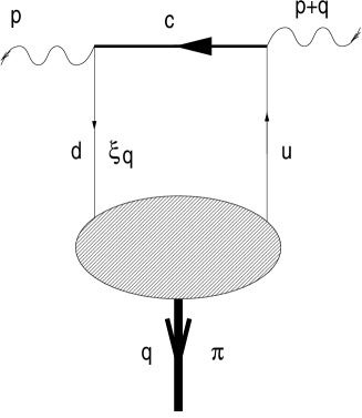
Figure 20: Light cone sum rule for $D^{*}D\pi$ in the leading order. The current labeled by $p+q$ interpolates $D$ while that labeled by $p$ interpolates $D^{*}$.

If $\xi$ is the fraction of the pion momentum carried by the $d$ quark, the graph of Fig. 20 gives rise to the following expression:

$$F_{\mu}\equiv q_{\mu}\,F(p^{2},(p+q)^{2})=m_{c}f_{\pi}q_{\mu}\,\int_{0}^{1}d\xi\,\frac{\phi_{\pi}(\xi)}{m_{c}^{2}-(p+\xi q)^{2}}\,+\,...\,,$$ (86)

where $\phi_{\pi}(\xi)$ is the distribution function, and the ellipses denote corrections, both perturbative (the $\alpha_{s}$ expansion) and non-perturbative (due to higher twists). The $c$ quark Green’s function is substituted, in the leading approximation, by that of a free quark. Emission of gluons from this line would result either in $\alpha_{s}$ corrections or in the distribution functions of non-leading twists.

For very small values of $q$ one could have substituted the denominator in Eq. (86) by $m_{c}^{2}-p^{2}$. Then the integral $\int d\xi\phi_{\pi}(\xi)\rightarrow 1$, and $F_{\mu}$ would reduce to the matrix element of the operator $\bar{d}\gamma_{\mu}\gamma_{5}u$ sandwiched between the pion state and vacuum.

Expanding the denominator in Eq. (86) in $q$ we readily identify higher dimension operators that are summed over: the term linear in $q$ originates from $\bar{d}\stackrel{{\scriptstyle\leftarrow}}{{D}}_{\alpha}\gamma_{\mu}\gamma_{5}u$, quadratic in $q$ from $\bar{d}\stackrel{{\scriptstyle\leftarrow}}{{D}}_{\alpha}\stackrel{{\scriptstyle\leftarrow}}{{D}}_{\beta}\gamma_{\mu}\gamma_{5}u$, etc. The actual expansion parameter is

$$\frac{pq}{p^{2}-m_{c}^{2}}\sim 1\,.$$

The (leading twist) light-cone wave function $\phi_{\pi}(\xi)$ is formally defined as

$$\langle\pi(q)|\bar{d}(x)\gamma_{\mu}\gamma_{5}\exp\{ig\int_{0}^{x}A_{\alpha}(y)dy_{\alpha}\}u(0)|0\rangle=-iq_{\mu}f_{\pi}\int_{0}^{1}\,d\xi\,e^{i\xi qx}\phi_{\pi}(\xi)\,.$$ (87)

It parametrizes the large-distance dynamics of the $\bar{d}u$ pair.

If we do the double Borel transformation, with respect to $p^{2}$ and $(p+q)^{2}$ the denominator in Eq. (86) becomes

$$\frac{M_{1}^{2}M_{2}^{2}}{M_{1}^{2}+M_{2}^{2}}\,\exp\left(-m_{c}^{2}\frac{M_{1}^{2}+M_{2}^{2}}{M_{1}^{2}M_{2}^{2}}\right)\delta\left(u-\frac{M_{1}^{2}}{M_{1}^{2}+M_{2}^{2}}\right)\,,$$ (88)

where $M_{1,2}$ are the corresponding Borel parameters, that are expected to lie close to each other inside the window. The sum rule is obtained by matching the double Borel transform of Eq. (85) with the double Borel transform of Eq. (86). Thus, we see that the theoretical part of the sum rule is determined by $\phi_{\pi}(0.5)$. Of course, there are corrections of higher order in $\alpha_{s}$ and from higher twist distribution functions, but as usual inside the window they should be kept at a modest level. In addition we must check the stability of the result inside the window. Provided all this is properly done, one obtains [79] $g$ in terms of $\phi_{\pi}(0.5)$. The latter quantity must be extracted from independent sources.

(The situation we face here is not quite generic. A priori one could expect the coupling $g$ to be expressible in terms of $\phi_{\pi}(\xi)$, rather than one constant, $\phi_{\pi}(0.5)$.)

Information on $\phi_{\pi}(\xi)$ is quite abundant; there is some limited information on the higher-twist wave functions too. The issue of $\phi_{\pi}(\xi)$ is almost as old as the SVZ sum rules themselves. The key element of the corresponding theory, which was studied in great detail in connection with hard exclusive processes, is the (approximate) conformal symmetry of QCD. Other elements are provided by the sum rule and lattice calculations and models. The issue is not completely settled, although it seems that a heated debate of the 1980’s gradually wanes. Out of two competing scenarios – a double hump distribution function of Chernyak and Zhitnitsky [78] and a narrow distribution of Radyushkin and collaborators [80] that is close to the asymptotic form of $\phi_{\pi}(\xi)$ – the second is gaining more recognition now. Experts lean towards a narrow almost asymptotic distribution. As usual, the best strategy is sacrificing one of the sum rules in order to extract $\phi_{\pi}(\xi)$ from data. A recent attempt based on the $\gamma^{*}+\gamma\rightarrow\pi^{0}$ data has been undertaken in Ref. [81]. I will not go into further details here, referring the reader to a very rich original literature devoted to this topic.

It remains to be added that (i) the term “light-cone sum rules” first appears in [82]; (ii) the idea of the approach dates back to Refs. [83]; and (iii) a review of this topic, with a representative list of references was published recently [84].

If the partial summation of the higher-dimension operators turns out to be so successful in the light-cone sum rules, it is natural to ask [85] why it is not applied in the vacuum correlation functions appearing in the SVZ sum rules. In this case, in order to partially sum, say, the quark operators we must substitute the quark condensate $\langle\bar{q}q\rangle$ by a “ string expectation value” in the vacuum,

$$\langle\bar{q}(x)\,\exp\{ig\int_{0}^{x}A_{\alpha}(y)dy_{\alpha}\}q(0)\rangle\,,$$ (89)

which is a function of $x$.

In the light cone sum rules one can ascribe certain twist to each given distribution function. Each distribution function sums up a tower of the local operators, with all dimensions but given twist. Therefore, the distribution functions can be systematically ordered in twist. Twist is obviously irrelevant in the vacuum correlation functions. Therefore, the partial summation implemented by the “string expectation values” (89) is hard to justify theoretically. A principle that would allow us to order distinct “string expectation values” has to be elaborated.

Another major difference with the light cone sume rules is that the pion distribution function is known at least at a certain level, while next to nothing is known about the vacuum function (89). Until recently even the large $x$ asymptotic behavior of this function was erroneously assumed to be Gaussian. We are at the initial stage, when first observations are being made regarding properties of the function (89) following from the general structure of QCD [16]. I do not rule out that, as our understanding progresses, the corresponding modification of the sum rule approach will be elaborated.

10.2 Heavy flavor sum rules

Although the character of problems in which this formalism is instrumental is somewhat different from the classical applications of the SVZ sum rules, the basic techniques – OPE, matching of the theoretical expansions with the phenomenological expressions represented by dispersion integrals over the observable spectral densities, etc. – are the same. The vacuum condensates are replaced by the expectation values of local operators over the heavy flavor states, say, $B$ mesons. All questions that can be asked in connection with the vacuum condensates exist here too; the answers are more transparent, however. We will consider below a sample application. Our main goal is discussing subtle nuances associated with the condensate expansion (Wilsonean OPE versus practical version, see Sect. 6).

The heavy flavor sum rules were engineered [19] to treat the inclusive heavy flavor decays, for instance the semileptonic decays $B\rightarrow X_{c}\ell\nu$ where $X_{c}$ is arbitrary hadronic state containing $c$ quark. The lowest-lying state is the $D$ meson, then comes $D^{*}$ and then higher excitations/continuum. By varying the momentum of the lepton pair one can measure various spectra in the transition $b\rightarrow c$ induced by the weak current. The object of the theoretical study is the transition operator

$${\hat{T}}_{ab}(q)=i\int d^{4}x\;{\rm e}^{iqx}\,T\{j_{a}^{\dagger}(x)j_{b}(0)\}\,,$$ (90)

that will be eventually sandwiched between the states $|B\rangle$ and $\langle B|$ (see Fig. 21). Here $j_{a}$ denotes a current of the type $\bar{c}\Gamma_{a}b$ with an arbitrary Dirac matrix $\Gamma_{a}$; $q$ is the momentum carried away by the lepton pair.

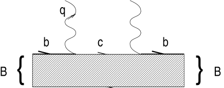
Figure 21: The operator product expansion for $h_{ab}$. For large negative $\epsilon$ the $c$ quark is far off shell, and the points of the current emission and absorption are close. The $B$ meson in the initial and final states is assumed to be at rest.

The average of ${\hat{T}}_{ab}$ over the heavy hadron state $B$ with the momentum $p_{B}$ represents a forward scattering amplitude (the so-called hadronic tensor),

$$h_{ab}(p_{B},q)=\frac{1}{2M_{B}}\langle B|\hat{T}_{ab}|B\rangle\;.$$ (91)

The structure functions $w_{ab}$ are obtained from the hadronic tensor by taking its imaginary part,

$$w_{ab}=(1/i)\,{\rm disc}\,\,h_{ab}\,.$$

All observable spectra are represented as certain integrals over $w_{ab}$. The hadronic tensor $h_{ab}$ and the structure functions $w_{ab}$ can be expanded in terms of various kinematic structures. For each set of the currents generically we may have up to five distinct kinematic structures; these details need not bother us here. For illustrational purposes it is sufficient to limit ourselves to the axial currents, so that $\Gamma_{a,b}\rightarrow\gamma_{\mu}\gamma_{5}$, and to the first function,

$$h_{\mu\nu}=-h_{1}g_{\mu\nu}+...\,,\,\,\,w_{1}=(1/i)\,{\rm disc}\,\,h_{1}\,.$$

The lowest-lying state produced by the axial current from $B$ is $D^{*}$. To end up with the kinematical aspects we must specify the lepton pair momentum $q$. It will be assumed that the spatial momentum $\vec{q}$ is small but non-vanishing, $\Lambda\ll|\vec{q}|\ll M_{D}$. The terms ${\cal O}({\vec{q}}^{2})$ will be kept while those of higher order in $|\vec{q}|$ will be neglected. Since $\vec{q}$ is fixed, $h_{1}^{AA}$ becomes a function of one (complex) variable, $q_{0}$. Instead of $q_{0}$ it is more convenient to work with $\epsilon$ defined as

$$\epsilon=q_{0max}-q_{0}$$ (92)

where

$$q_{0max}=M_{B}-E_{D^{*}},\,\,\,E_{D^{*}}=M_{D^{*}}+\frac{{\vec{q}}^{2}}{2M_{D^{*}}}.$$ (93)

When $\epsilon$ is real and positive we are on the physical cut where the imaginary part of $h_{1}^{AA}$ is measurable. For negative $\epsilon$ we are below the cut, in the Euclidean domain, where the $T$ product (90) can be computed as an expansion in $1/m_{c,b}$. The leading operator in this expansion is $\bar{b}b$. It has dimension three. No operators of dimension four exist. At the next level, of dimension five, there are two operators, $\bar{b}(i\vec{D})^{2}b$ and $(ig/2)\bar{b}\gamma^{\mu}\gamma^{\nu}G_{\mu\nu}b$. The first operator (sometimes called the kinetic energy operator) is not a Lorentz scalar. In the problem considered the operators to be retained in the expansion need not necessarily be Lorentz scalars since, unlike the vacuum case, the very presence of the $B$ meson in the initial/final state singles out a reference frame.

The whole procedure is perfectly analogous to the $1/Q^{2}$ expansion of the polarization operator discussed in Sect. 4. The operator $\bar{b}b$ occupies the same position in the hierarchy as the unit operator in the expansion of the vacuum correlators. The operators of dimension five and higher generate $1/m_{c,b}$ corrections analogous to the condensate corrections. In the problem at hand all local operators appearing in the expansion of the $T$ product (90) are averaged over the $B$ meson state. In this way we get a theoretical expression for $h_{1}^{AA}$ off the cut.

A bridge between $h_{1}^{AA}$ at negative $\epsilon$ and $w_{1}^{AA}$ at positive $\epsilon$ is provided by the dispersion relation. Expanding the denominator in the dispersion relation in $1/\epsilon$ we obtain an infinite set of the sum rules. The third of them is as follows [86]:

$$\frac{1}{2\pi}\int d\epsilon\,\epsilon^{2}\,w_{1}^{AA}(\epsilon)=\frac{1}{3}\mu_{\pi}^{2}\,{\vec{v}}^{2}+...\,.$$ (94)

Here $\vec{v}$ is the velocity of the produced heavy hadron (in the $B$ rest frame), and $\mu_{\pi}^{2}$ is defined as the expectation value

$$\mu_{\pi}^{2}=\frac{1}{2M_{B}}\langle B|\bar{b}(i\vec{D})^{2}b|B\rangle\,.$$ (95)

This parameter, $\mu_{\pi}^{2}$, has the meaning of the average spatial momentum squared of the heavy quark inside $B$ meson, and is one of the fundamental parameters of the heavy quark theory. One encounters $\mu_{\pi}^{2}$ in a large number of applied problems. It is fair to say that in the heavy quark physics $\mu_{\pi}^{2}$ plays the same role as the gluon condensate in classical applications of the SVZ method.

The ellipses in Eq. (94) denote corrections suppressed by powers of $1/m_{c,b}$. Since the weight function in Eq. (94) is proportional to $\epsilon^{2}$, the “elastic” $B\rightarrow D^{*}$ transition drops out, and the integral on the left-hand side is saturated by “inelastic” transitions, i.e. decays of the $B$ meson in the excited $X_{c}$ states. For such transitions $w_{1}^{AA}(\epsilon)$ is proportional to ${\vec{v}}^{2}$ at $|{\vec{v}}|\ll 1$. It is convenient then to introduce a spectral function $\sigma(\epsilon)$ which does not vanish in the limit $|{\vec{v}}|\rightarrow 0$,

$$\sigma(\epsilon)=|{\vec{v}}|^{-2}w_{1}^{AA}(\epsilon)\,,\,\,\,\epsilon>0\,.$$ (96)

Our brief excursion in the heavy flavor sum rules is almost over. In terms of the new spectral density the sum rule we are interested in takes the form

$$\frac{1}{2\pi}\int d\epsilon\epsilon^{2}\,\sigma(\epsilon)=\frac{1}{3}\mu_{\pi}^{2}\,.$$ (97)

As with any sum rule it can be read in both directions: if $\mu_{\pi}^{2}$ is known this is a prediction for the spectral density. On the other hand, if the spectral density is measured we can take the integral and get $\mu_{\pi}^{2}$. Below we will pursue the latter strategy assuming that $\sigma(\epsilon)$ is measured. In actuality this is not the case, but we have a pretty good idea of how $\sigma(\epsilon)$ will look like when it is measured. First of all, it is positive-definite. At small values of $\epsilon$, of order of a few units time $\Lambda$, there is one, perhaps, two resonances; then at higher values of $\epsilon$ the spectral density must approach its perturbative asymptotics which is known too: $\sigma(\epsilon)\rightarrow C\alpha_{s}/\epsilon$, where $C$ is a constant which was calculated in Ref. [19]. The numerical value of $C$ is unimportant for our purposes. The asymptotic regime is achieved through oscillations – the reasons are the same as in Sects. 2.2 and 4. A schematic plot of $\epsilon^{2}\sigma(\epsilon)$ is depicted in Fig. 22.

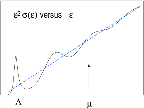
Figure 22: A sketch of $\epsilon^{2}\sigma(\epsilon)$ in the $b\rightarrow c$ transition at small $|\vec{v}|$ (solid curve). The spectral density $\sigma(\epsilon)$ is defined in Eq. (96). The dashed curve represents $\epsilon^{2}\sigma(\epsilon)$ in perturbation theory at one loop.

If you think about Eq. (97) you will, probably, find it remarkable: it gives a condensate-like non-perturbative parameter in terms of an integral over the observable spectral density. Further examination raises a question. Indeed, if the integral extends to infinity, it badly diverges.

One need not be concerned, however. This infinity reflects the fact that the proper definition of $\mu_{\pi}^{2}$ requires a normalization point, just in the same way as the for the gluon condensate. In the case at hand this normalization point has a very transparent physical meaning – $\mu$ is the maximal excitation energy of the hadronic state belonging to the class of “soft excitations” (Fig. 22). Higher excitations are considered to be hard, and are well approximated by perturbation theory. I remind that the hard contributions do not belong to $\mu_{\pi}^{2}$; rather, they determine the coefficient functions in OPE. In the perturbative calculation of the coefficient functions one must remove the part with $\epsilon<\mu$. In fact, the cut off in the excitation energy as a normalization point was suggested in the given context long ago in Ref. [87]. Thus, in the Wilsonean approach $\mu_{\pi}^{2}(\mu)$ is determined as

$$\mu_{\pi}^{2}(\mu)=\frac{3}{2\pi}\int_{0}^{\mu}d\epsilon\epsilon^{2}\,\sigma(\epsilon)\,.$$ (98)

In practical OPE we deal, instead, with subtracted “surrogates”. Say, if one limits oneself to one-loop accuracy,

$$``\mu_{\pi}^{2}"=\frac{3}{2\pi}\int_{0}^{\mu}d\epsilon\epsilon^{2}\,\left[\sigma(\epsilon)-\sigma_{\rm 1-loop}(\epsilon)\right]\,.$$

The right-hand side in this expression is $\mu$ independent at one loop. Its $\mu$ dependence shows up only at two loops. If we agree to discard all effects ${\cal O}(\alpha_{s}^{2})$ and higher, just totally ignore them, then the integration in $``\mu_{\pi}^{2}"$ can be extended to infinity. Correspondingly, the coefficient functions must be calculated at one-loop, following the standard Feynman rules, with no removal of the $\epsilon<\mu$ part.

11 Sum Rules and Lattices

In this Lecture it has been already noted, more than once, that certain aspects of the condensate approach, as well as a rich experience in the analysis of various spectral densities, might be useful for lattice practitioners. Remarks to this effect are scattered here and there. Of particular importance are qualitative observations, such as an enhanced sensitivity to the vacuum fermion loops in certain channels (this effect is neglected in the quenched approximation), the existence of new, abnormally large scales in the $0^{\pm}$ glueball channels, and so on. Surprising though it is, all these hints, which might have produced a strong impact on the lattice theory, are so far almost totally ignored . The reaction of rejection of any ideas coming from outside the lattice theory per se plagues the lattice community. This happens even in those cases where the overlap is quite obvious.

Let me give an almost anecdotal example. As was mentioned in Sect. 7, in 1981 a wide class of “QCD scale anomaly” low-energy theorems was obtained [3] in connection with the SVZ sum rules. These theorems relate to each other $n$-point functions with arbitrary number of insertions of the operator $\sigma(x)=\theta^{\mu}_{\mu}(x)\,\propto G^{2}$ (see Eq. (39)) at vanishing momentum. One of this theorems can be cast in the form of a prediction for the expectation value of $G_{\mu\nu}^{2}$ in the presence of the Wilson loop operator $W$,

$$\left\langle W\right\rangle^{-1}\left\langle\int d^{3}x\sigma(x)W\right\rangle_{\rm E,c}=V(R)+R\frac{\partial V(R)}{\partial R}$$ (99)

where $V(R)$ is the static potential between the heavy quarks separated by distance $R$,

$$W=\oint_{C}\,\mbox{Tr}\,\exp(igA_{\mu}(x)dx_{\mu})\,,$$

the contour $C$ in the definition of the Wilson loop is depicted on Fig. 23, and the subscript E reminds us that all definitions and calculations refer to the Euclidean space. Moreover, the integration in Eq. (99) is performed in three directions perpendicular to the Euclidean time; the subscript c refers to the connected part, i.e. the disconnected part of the correlation function (99) must be discarded. One can interprete the operator $\sigma(x)$ in Eq. (99) as a probe of the energy density of the vacuum medium at the point $x$ in the presence of a pair of heavy static quark sources separated by distance $R$ [3]. In the case of purely linear potential the right-hand side reduces to $2V(R)$. In this form the theorem (99) was derived in Ref. [3] (see Appendix B). The generalization to the case of arbitrary potentials is due to Dosch et al. [89].

Figure 23: Rectangular contour in the Wilson loop operator. One can consider it as a trajectory of infinitely heavy quarks (in the imaginary time). $R$ is the distance between the quark and antiquark, $T\rightarrow\infty$.

Derivation of the theorem (99) is very similar to other theorems discussed in Sect. 7. The functional-integral representation for $\langle W\rangle$ is differentiated with respect to $1/g_{0}^{2}$. We then use the fact that

$$\frac{\partial V(R)}{\partial(1/4g_{0}^{2})}=-\frac{32\pi^{2}}{b}\left(V(R)+R\frac{\partial V(R)}{\partial R}\right)\,.$$ (100)

The latter equality, in turn, follows from consideration similar to that presented in Sect. 7. Thus, the low-energy theorem (99) is a reflection of the scale anomaly of QCD, and as such, represents a fundamental aspect of the theory.

Now I come to a culmination of the story. In 1987 the theorem (99) was rediscovered in the lattice community [90], where it goes under the name of the “action Michael sum rule”. The original derivation was erroneous, the second term on the right-hand side of Eq. (99) was omitted. The error was corrected in Ref. [89] which was specifically devoted to the issue. Nevertheless, the theorem continues to circulate in the lattice community as the “Michael sum rule” , see e.g. [91].

This example of a “lattice xenophobia” is by no means unique. Needless to say that I consider the situation as absolutely unhealthy. The problems we face in the hadronic world are too complicated to afford neglecting the work done in related areas. The analytic and numerical approaches should complement each other. I sincerely hope that the attitude of the lattice community will start changing after recent breakthrough discoveries in supersymmetric gauge theories. Supersymmetry is a powerful tool which allows us to reveal features of strong coupling gauge dynamics we never suspected of. One of the lessons which seems undeniable is the proof that massless (or light) quarks play much more significant a role than is universally believed among the lattice practitioners. In the quenched approximation, the most wide spread today, the dynamical quarks are neglected altogether. Even the most advanced lattice investigations, which do not rely on the quenched approximation, routinely use extrapolations in the number of the massless quarks. Supersymmetric gauge theories teach us that increasing the number of massless quarks from two to three or changing the color representation of the fermion fields from fundamental to adjoint is not necessarily a smooth process. Dynamics may change drastically!

Penetration of ideas and insights obtained analytically, in the practice of lattice calculations, where they can be used, at the very least, to test reliability of various approximations, is unavoidable. First steps in this direction have been already reported [92].

12 Vacuum Fluctuations Are Subtle Creatures

The rich SVZ phenomenology confirms the wide-spread belief that the structure of the hadronic family, in all its gross features and intricacies, derives from a complicated organization of the vacuum medium. The vacuum fluctuations are violent, but fine-tuned in a very specific way. Within the method, as it exists today, we do not calculate the vacuum condensates. This does not mean, of course, that the origin of the condensates, and their relative values, are of no interest. I merely wanted to say that the problem of the vacuum structure in analytic QCD is not solved in full. There are indirect methods, however, which show that this structure is very subtle – much more subtle than one might think of a priori – and depends on seemingly insignificant details of the theory. For instance, changing the number of colors from three to two dramatically changes the pattern of the spontaneous chiral symmetry breaking resulting in a drastic rearrangement in the Goldstone sector of the hadron family. Instead of $N_{f}^{2}-1$ QCD “pions” ($N_{f}$ stands for the number of the light quark flavors) we get $2N_{f}^{2}-N_{f}-1$ massless Goldstone hadrons . This conclusion can be achieved [93] from consideration of the ’t Hooft matching conditions [94] (for earlier analyses based on less rigorous arguments see Ref. [95]).

Let us dwell on this issue. Assume that we have $N_{f}$ massless (light) quarks but the color gauge group is $SU(2)$. The quarks belong to the fundamental representation of $SU(2)$. Unlike QCD, in which the color triplets and antitriplets are independent representations, the $SU(2)$ doublets are essentially the same as antidoublets. In other words, all representations of $SU(2)$ are (quasi)real.

This simple observation has far reaching consequences. Indeed, the flavor symmetry of the Lagrangian is $SU(2N_{f})$ now, rather than $SU(N_{f})\times SU(N_{f})$ we deal with in QCD. Out of $4N_{f}^{2}-1$ currents $2N_{f}^{2}-N_{f}-1$ are axial; all correspond to the spontaneously broken symmetries since there is no way one can achieve the matching of the triangular AVV anomalies otherwise [93]. This means that the pattern of the chiral symmetry breaking is $SU(2N_{f})\rightarrow Sp(2N_{f})$ rather than the $SU(N_{f})\times SU(N_{f})\rightarrow SU(N_{f})$ we got used to in QCD. The very gross features of the vacuum structure do depend on the number of colors!

Not only do they depend on the number of colors, they are also sensitive to the fermion contents of the theory.

Indeed, let us substitute the standard quarks of QCD with one Majorana fermion $\lambda$ in the adjoint representation of the color group. The theory thus obtained is nothing but supersymmetric gluodynamics. Superficially it looks very similar to conventional QCD. At first sight, one can hardly expect any conspicuous deviations from the conventional pattern of behavior.

It has been known for many years that the supersymmetric gauge theories posses some miraculous properties. In particular, in supersymmetric gluodynamics the Gell-Mann–Low function is known exactly [96]

$$\beta(\alpha_{s})=-\frac{\alpha^{2}_{s}}{2\pi}\,\,\frac{3N}{1-(N\alpha_{s}/2\pi)}\,,$$ (101)

where the $SU(N)$ gauge group is assumed.

As QCD, supersymmetric gluodynamics is believed to be confining in the infrared domain. Unlike QCD, however, the condensate $\langle\lambda^{2}\rangle$ may or may not develop. It was argued recently [97] that two distinct phases coexist in this theory – the conventional chirally asymmetric phase with $\langle\lambda^{2}\rangle\neq 0$, that reminds QCD, and a very unusual chirally symmetric phase where $\langle\lambda^{2}\rangle=0$. The arguments leading to this conclusion are too technical to be reproduced here. They would lead us far astray. The interested reader is referred to Ref. [97].

Instead, let us dwell on another example which is pretty close to actual QCD. In fact, we will consider just conventional QCD with more than three massless flavors.

The Gell-Mann-Low function in QCD has the form [6]

$$\beta(\alpha_{s})=-b\frac{\alpha_{s}^{2}}{2\pi}-b_{1}\frac{\alpha_{s}^{3}}{4\pi^{2}}-...\,,$$

$$b=11-\frac{2}{3}N_{f}\,,\,\,\,b_{1}=51-\frac{19}{3}N_{f}\,.$$ (102)

At small $\alpha_{s}$ it is negative (asymptotic freedom!) since the first term always dominates. With the scale $\mu$ decreasing the running gauge coupling constant grows, and the second term becomes important. Generically the second term takes over the first one at $\alpha_{s}/\pi\sim 1$, when all terms in the $\alpha_{s}$ expansion are equally important, i.e. in the strong coupling regime. We do not know what exactly happens at $\alpha_{s}/\pi\sim 1$. Assume, however, that for some reasons the first coefficient $b$ is abnormally small, and this smallness does not propagate to higher orders. Then the second term catches up with the first one when $\alpha_{s}/\pi\ll 1$, we are in the weak coupling regime, and higher order terms are inessential. Inspection of Eq. (102) shows that this happens when $N_{f}$ is close to $33/2$, say 16 or 15 ($N_{f}$ has to be less than $33/2$ to ensure asymptotic freedom). For these values of $N_{f}$ the second coefficient $b_{1}$ turns out to be negative. This means that the $\beta$ function develops a zero in the weak coupling regime, at

$$\frac{\alpha_{s}^{*}}{2\pi}=\frac{b}{-b_{1}}\ll 1\,.$$ (103)

(Say, if $N_{f}=15$ the critical value is at 1/44 and is indeed small.) This zero is nothing but the infrared fixed point of the theory. At large distances $\alpha_{s}\rightarrow\alpha_{s}^{*}$, and $\beta(\alpha_{s}^{*})=0$, implying that the trace of the energy-momentum vanishes. Then the theory is in the conformal regime. There are no localized particle-like states in the spectrum of this theory; rather we deal with massless unconfined interacting quarks and gluons; all correlation functions at large distances exhibit a power-like behavior. In particular, the potential between two heavy static quarks at large distances $R$ will behave as $\sim\alpha_{s}^{*}/R$, i.e. we have a pure Coulomb behavior. The situation is not drastically different from conventional QED. As long as $\alpha_{s}^{*}$ is small, the interaction of the massless quarks and gluons in the theory is weak at all distances, short and large, and is amenable to the standard perturbative treatment (renormalization group, etc.). The chiral symmetry is not broken spontaneously, the quark condensates do not develop. QCD becomes a fully calculable theory.

The fact that at $N_{f}$ close to 16 QCD becomes conformal and weakly coupled in the infrared limit is known for about 20 years [98, 99]. If the conformal regime takes place at $N_{f}=16$ and 15, let us ask ourselves how far can we descend in $N_{f}$ without ruining the conformal nature of the theory in the infrared? Certainly, when $N_{f}$ is not close to 16 the gauge coupling $\alpha_{s}^{*}$ is not small. The theory is strongly coupled, as conventional QCD, and, simultaneously, conformal in the infrared. The chiral symmetry presumably is unzbroken, $\langle\bar{q}q\rangle=0$. The vacuum structure is totally different, and so are all properties of the theory.

The range of $N_{f}$ where this phenomenon occurs is called the conformal window. The right edge of the conformal window is at $N_{f}=16$. There are indications that the left edge of the conformal window $N_{f}^{*}$ lies not too far from actual QCD (i.e. not too far from $N_{f}=3$).

First, in the instanton liquid model it was found [100] that at $N_{f}=5$ the chiral condensate disappears, $\langle\bar{q}q\rangle=0$. Although nothing is said about the onset of the conformal regime in this work, the vanishing of $\langle\bar{q}q\rangle$ may be a signal. More definite is the conclusion of the lattice investigation [101]. It is claimed that at $N_{f}=7$ not only the quark condensate disappears, $\langle\bar{q}q\rangle=0$, but the decay law of the correlation functions at large distances changes from the exponential to power-like, i.e. the theory switches from the confining regime to the conformal one. One could speculate that at $N_{f}=5$ and 6 we are in the intermediate phase, when confinement is still operative at large distances but the chiral symmetry is unbroken. Previously it was believed that that confinement of color in QCD implies the chiral symmetry breaking [102]. Today’s wisdom tells us that this need not be necessarily the case. At least in some supersymmetric gauge theories we have both: confinement and unbroken chiral symmetry (see e.g. [97]). In any case, we see that ascending from $N_{f}=3$ to $N_{f}=5$ or 7 – quite a modest variation– we drastically change the vacuum structure of the theory, with the corresponding abrupt change of the picture of the hadron world.

An interesting question is what happens slightly below the left edge of the conformal window $N_{f}^{*}$. If $N_{f}$ were a continuous parameter, and the phase transition in $N_{f}$ were of the second order, slightly below $N_{f}^{*}$ the string tension $\sigma$ would be parametrically small in its natural scale given by $\Lambda^{2}$. In actuality $N_{f}$ changes discretely. Still it may well happen that at $N_{f}=N_{f}^{*}-1$ the ratio $\sigma/\Lambda^{2}$ is numerically small. This would mean that the string and its excitations, whose scale is set by $\sigma$, are abnormally light. Under the circumstances one might hope to build effective low-energy approaches analogous to the chiral Lagrangians of actual QCD. In the limit $\sigma/\Lambda^{2}\rightarrow 0$ the string becomes, in a sense, classic; the quantum corrections are unimportant. I do not rule out that the string representation of QCD – the holy grail of two generations of theorists – is easier to construct in this limit. One could even dream of an expansion in $N_{f}^{*}-3$. At this moment, this is a pure speculation, however, and I have to wind up.

13 Instead of Conclusions

As time passes the hopes that the full analytic solution of QCD will be found fade away. After all, the problem is with us for over a quarter of the century, and none of numerous theoretical attacks reached the goal. Many theorists whose philosophy is “all or nothing” abandoned the field . Does it mean that the theory of hadrons is an aging science at the verge of submerging into a permanently dormant state?

I do not think so. Those theorists who stayed in the field can claim many partial successes. The field is messy and down-to-earth but – what can we do? – this is the only world God gave to us. The theory of hadrons is alive. Our understanding of the vacuum structure of quantum chromodynamics and various dynamical regimes it can support continues to grow. Especially fruitful were the last years, with many breakthrough discoveries in supersymmetric gauge theories. These discoveries are to be used as hints and insights in actual QCD.

OPE-based methods – and the SVZ sum rules is one of them – continue to grow too. They are admittedly approximate, but their analytic nature and a graphic physical interpretation make them indispensable in many practically important problems. In some issues they share their role with other methods, which were developed later, for instance, lattice QCD. Since the theory of hadrons is so difficult it is in our best interests to combine all sources of information. We are in no position to neglect one of them in favor of the other. Many ideas and theoretical devices surfaced in connection with the SVZ method (e.g. the low-energy theorems, Sect. 7); the method also produced a number of variations and spin-offs. This is a healthy process which will hopefully continue.

14 Appendix. Some Useful Definitions and Formulae.

The Gell-Mann–Low function is defined as

$$\frac{\partial\alpha_{s}}{\partial\ln\mu}\equiv\beta(\alpha_{s})=-b\frac{\alpha_{s}^{2}}{2\pi}-b_{1}\frac{\alpha_{s}^{3}}{4\pi^{2}}+...$$ (A.1)

This definition is standard except that in some sources the first coefficient is called $\beta_{0}$, the second $\beta_{1}$, and so on (cf. Ref. [6]). At two loops the $\beta$ function is scheme independent.

The coefficients are

$$b=11-\frac{2}{3}\,N_{f}\,,\,\,\,b_{1}=51-\frac{19}{3}\,N_{f}\,.$$ (A.2)

The running coupling $\alpha_{s}(\mu)$ is parametrized as follows

$$\alpha_{s}(\mu)=\frac{4\pi}{b\,\ln\frac{\mu^{2}}{\Lambda^{2}}}\,\left(1-\frac{2b_{1}}{b^{2}}\,\frac{\ln\ln\frac{\mu^{2}}{\Lambda^{2}}}{\ln\frac{\mu^{2}}{\Lambda^{2}}}+...\right)\,.$$ (A.3)

A more convenient form of the very same expression is

$$\frac{2\pi}{\alpha_{s}(\mu)}=b\,\ln\frac{\mu}{\Lambda}+\frac{b_{1}}{b}\ln\ln\frac{\mu^{2}}{\Lambda^{2}}+...\,.$$ (A.4)

Being expanded, at two loops, the latter expression is equivalent to the former; Eq. (A.4) effectively sums up some higher order terms.

The scale parameter $\Lambda$ following from Eq. (A.3) is

$$\Lambda^{b}=\left(\frac{2}{b}\right)^{b_{1}/b}\mu^{b}\exp\left\{-\left[\frac{2\pi}{\alpha_{s}(\mu)}-\frac{b_{1}}{b}\,\ln\frac{2\pi}{\alpha_{s}(\mu)}\right]\right\}\,.$$ (A.5)

The first factor on the right-hand side is an (inconvenient) artifact of the definition. It could have been easily avoided. Since the definition is standard, we will keep it not to cause confusion.

Perturbative calculations in QCD, as a rule, are carried out in the so called modified minimal subtraction ($\overline{\rm MS}$) scheme [103], using dimensional regularization. For massless quarks and gluons it works nicely; the treatment of the heavy quark mass thresholds in this approach is ugly. The most common is the step-function approximation [104]: immediately above the threshold the quark is declared massless, while below the threshold it is treated as infinitely heavy, so that it is frozen out and does not participate in loops. This is equivalent to treating $N_{f}$ as a function of $\mu$ constructed from several step functions, $N_{f}=3$ below $m_{c}$, then it jumps to $N_{f}=4$ between $m_{c}$ and $m_{b}$, etc. Matching conditions at thresholds require equivalence of one effective theory with $N_{f}$ massless quarks to another effective theory with $N_{f}-1$ massless quarks.

If the step-function approximation is applied, at one loop the coupling constant is obviously continuous, while the first $\mu$ derivative experiences a jump. At two and three loops the coupling itself becomes discontinuous if the matching is done at the quark masses [105]. Several suggestions as to how one can smooth out the running coupling constant using various “physical” definitions were presented in the literature [106]. I propose a somewhat different approach inspired by supersymmetry. In supersymmetric theories the quark mass thresholds can be accounted for exactly, to all orders [107]. For instance, consider supersymmetric QCD with one flavor, with the mass term $m$. Assume that we start our evolution at a high normalization point $M_{0}$ (the corresponding coupling constant is $\alpha_{s0}$), pass the threshold and descend down to $\mu\ll m$. A continuously running $\alpha_{s}$ can be obtained from the formula

$$\frac{2\pi}{\alpha_{s}(\mu)}=\frac{2\pi}{\alpha_{s0}}-3N\ln\frac{M_{0}}{\mu(\alpha_{s0}/\alpha_{s}(\mu))^{1/3}}+\ln\frac{M_{0}}{\mu Z(\mu)}\,,$$ (A.6)

for SU(N) gauge group. Here $Z(\mu)$ is the $Z$ factor of the matter fields and $\mu$ is arbitrary: larger or smaller than $m$. At $\mu=m$ and below the second logarithm freezes at $\ln M_{0}/m_{0}$ where $m_{0}=mZ$ is the mass parameter normalized at $M_{0}$. The one loop $Z$ factor implies $\alpha_{s}(\mu)$ at two loops. Needless to say that $Z(\mu)$ varies continuously at one loop. At the two-loop level the high- and low-energy scale parameters are related as follows:

$$\Lambda_{\rm LOW}^{3N}=\Lambda_{\rm HIGH}^{3N-1}\left(\frac{2}{3N}\right)^{N}\left(\frac{3N-1}{2}\right)^{N-\frac{2C_{2}}{3N-1}}\,\left[m_{0}\left(\frac{2\pi}{\alpha_{s0}}\right)^{2C_{2}/(3N-1)}\right]\,,$$ (A.7)

where

$$C_{2}=\frac{N^{2}-1}{2N}\,.$$

At this level of accuracy $m_{0}$ and $\alpha_{s0}$ in the square brackets can be treated in the leading logarithmic approximation. In this approximation the expression in the square brackets is renormalization-group invariant. In principle, the procedure can be extended to all loops, but we will not pursue this goal here.

In non-supersymmetric QCD the exact treatment of the mass thresholds seems impossible. However, numerically the situation is quite close to what we have in supersymmetric QCD. One can work out compact formulae applicable at two loops. Say, for the charm threshold

$$\frac{2\pi}{\alpha_{s}(\mu)}=\frac{2\pi}{\alpha_{s0}}-9\ln\frac{M_{0}}{\mu(\alpha_{s0}/\alpha_{s}(\mu))^{32/81}}+\frac{2}{3}\ln\frac{M_{0}}{\mu Y(\mu)}\,,$$ (A.8)

where

$$Y=\left[\frac{\alpha_{s0}}{\alpha_{s}(\mu)}\right]^{3y/25}$$

and

$$y=\frac{107}{18}\,.$$

Correspondingly,

$$\Lambda_{\rm LOW}^{9}=\Lambda_{\rm HIGH}^{25/3}\left(\frac{2}{9}\right)^{32/9}\left(\frac{25}{6}\right)^{77/25}\,\left[m_{0}\left(\frac{2\pi}{\alpha_{s0}}\right)^{12/25}\right]^{2/3}\,\left[\frac{2\pi}{\alpha_{s}(m)}\right]^{7/45}\,.$$ (A.9)

If it were not for the last factor (which is quite close to unity) the relation between the low- and high-energy scales would be similar to that in supersymmetric QCD.

Matching at two thresholds, charm and beauty, yields

$$\Lambda_{\rm LOW}^{9}=\Lambda_{\rm HIGH}^{23/3}\left(\frac{2}{9}\right)^{32/9}\left(\frac{23}{6}\right)^{58/23}\,\left[m_{1}^{*}m_{2}^{*}\right]^{2/3}\,\left[\frac{2\pi}{\alpha_{s}(m_{2})}\right]^{21/115}\,\left[\frac{2\pi}{\alpha_{s}(m_{1})}\right]^{7/45}\,,$$ (A.10)

where

$$m_{i}^{*}=m_{i0}\,\left[\frac{2\pi}{\alpha_{s0}}\right]^{12/23}\,.$$

Recommended Literature

Two review papers

B.L. Ioffe, Acta Phys. Polon. B16 (1985) 543;

L.J. Reinders, H. Rubinstein, and S. Yazaki, Phys. Reports 127 (1985) 1

were published in the mid-1980’s. They may serve for an initial exposure but they do not provide an overview of modern developments. Neither do they reflect modern understanding of conceptual issues. A dedicated comprehensive review on this subject is long overdue.

A brief survey of the light-cone sum rules is given in

V. Braun, hep-ph/9801222.

SVZ sum rules in the heavy quark theory are discussed in

M. Neubert, Phys. Reports 245 (1994) 259.

For a review of the sum rule applications in weak decays see

A. Khodjamirian and R. Rückl, hep-ph/9801443.

Some topics related to the SVZ sum rules are covered in

M. Shifman, Phys. Reports 209 (1991) 341;

T. Schäfer and E. Shuryak, hep-ph/9610451 (Rev. Mod. Phys., to appear).

A collection of the original papers with an extended commentary reflecting the state of the art in the late 1980’s can be found in

Vacuum Structure and QCD Sum Rules, Ed. M. Shifman (North-Holland,

Amsterdam, 1992).

Some useful formulae are compiled in

S. Narison, QCD Spectral Sum Rules, (World Scientific, Singapore, 1989).

I do not agree with the treatment of many conceptual issues and technical details in this book.

References

- [1] M. Shifman, A. Vainshtein and V. Zakharov, Nucl. Phys. B147 (1979) 385; 448.
- [2] Vacuum Structure and QCD Sum Rules, Ed. M. Shifman (North-Holland, Amsterdam, 1992).
- [3] V. Novikov, M. Shifman, A. Vainshtein and V. Zakharov, Nucl. Phys. B191 (1981) 301.
-
[4]
D. Gross and F. Wilczek,
Phys. Rev. Lett. 30 (1973) 1343;
H. D. Politzer, Phys. Rev. Lett. 30 (1973) 1346. - [5] V. Novikov et al., Phys. Rep. 41 (1978) 1.
- [6] See e.g. the review paper I. Hinchliffe, Phys. Rev. D54 (1996) 77 and references therein.
-
[7]
G. ’t Hooft, The Confinement Phenomenon in Quantum Field
Theory, 1981 Cargese Summer School Lecture Notes on Fundamental
Interactions, Eds. M. Levy and J.-L. Basdevant, NATO Adv. Study
Inst. Series B: Phys. vol. 85, p. 639
[reprinted in G. ’t Hooft, Under the Spell of the Gauge Principle
(World Scientific, Singapore, 1994), p. 514];
S. Mandelstam, Phys. Reports 23 (1976) 245. - [8] For a review see e.g. A. Di Giacomo, Nucl. Phys. Proc. Suppl. 47 (1996) 136 [hep-lat/9509036]; Monopole Condensation in Gauge Theory Vacuum, in Confinement 95, Proc. International Workshop on Color Confinement and Hadrons Japan, March 1995, Eds. H. Toki, Y. Mizuno, H. Suganuma, T. Suzuki, O. Miyamura (World Scientific, Singapore, 1995) [hep-lat/9505006]; Mechanisms for Color Confinement, in Selected Topics in Nonperturbative QCD, Proc. Int. School of Physics “Enrico Fermi”, Eds. A. Di Giacomo and D. Diakonov (IOS Press, 1996), page 147.
- [9] N. Seiberg and E. Witten, Nucl. Phys. B426 (1994) 19; (E) B430 (1994) 485; Nucl. Phys. B431 (1994) 484.
-
[10]
G. ’t Hooft, Nucl. Phys. B72 (1974) 461;
E. Witten, Nucl. Phys. B160 (1979) 57;
for a brief review see Chapter 8 in Ref. [2]. -
[11]
A.B. Kaidalov, Usp. Fiz. Nauk 105 (1971) 97
[Sov. Phys. Uspekhi 14 (1972) 600];
P.D.B. Collins, An Introduction to Regge Theory and High Energy Physics (Cambridge Univ. Press, 1977). - [12] A.Yu. Dubin, A.B. Kaidalov, and Yu.A. Simonov, Phys. Lett. B323 (1994) 41.
- [13] A. Casher, N. Neurberger and S. Nussinov, Phys. Rev. D20 (1979) 179.
- [14] B. Blok, M. Shifman and Da-Xin Zhang, hep-ph/9709333 (Phys. Rev. D, to appear).
- [15] G. ’t Hooft, Nucl. Phys. B75 (1974) 461 [Reprinted in G. ’t Hooft, Under the Spell of the Gauge Principle (World Scientific, Singapore 1994), page 443]; see also F. Lenz, M. Thies, S. Levit and K. Yazaki, Ann. Phys. (N.Y.) 208 (1991) 1; C. Callan, N. Coote, and D. Gross, Phys. Rev. D13 (1976) 1649; M. Einhorn, Phys. Rev. D14 (1976) 3451; M. Einhorn, S. Nussinov, and E. Rabinovici, Phys. Rev. D15 (1977) 2282; I. Bars and M. Green, Phys. Rev. D17 (1978) 537.
- [16] M. Shifman, Theory of Preasymptotic Effects in Weak Inclusive Decays, in Proc. Workshop on Continuous Advances in QCD, ed. A. Smilga (World Scientific, Singapore, 1994), page 249 [hep-ph/9405246]; Recent Progress in the Heavy Quark Theory, in Particles, Strings and Cosmology, Proc. of the XIX Johns Hopkins Workshop on Current Problems in Particle Theory and the V PASCOS Interdisiplinary Symposium, Baltimore, March 1995, Ed. J. Bagger (World Scientific, Singapore, 1996), page 69 [hep-ph/9505289].
- [17] F. David, Nucl. Phys. B209 (1982) 433; B234 (1984) 237.
- [18] V. Novikov, M. Shifman, A. Vainshtein and V. Zakharov, Nucl. Phys. B249 (1985) 445.
- [19] I. Bigi, M. Shifman, N. Uraltsev and A. Vainshtein, Phys. Rev. D52 (1995) 196.
-
[20]
R. Crewther, Phys. Rev. Lett. 28 (1972) 1421;
M. Chanowitz and J. Ellis, Phys. Lett. B40 (1972) 397; Phys. Rev. D7 (1973) 2490;
J. Collins, L. Duncan and S. Joglekar, Phys. Rev. D16 (1977) 438. - [21] M. Neubert, Phys. Rev. D51 (1995) 5924.
- [22] P. Ball, M. Beneke, and V. Braun, Nucl. Phys. B452 (1995) 563.
- [23] G. ’t Hooft, Can We Make Sense out of “Quantum Chromodynamics”? in The Whys Of Subnuclear Physics, Erice 1977, ed. A. Zichichi (Plenum, New York, 1977), p. 943 [reprinted in G. ’t Hooft, Under the Spell of the Gauge Principle (World Scientific, Singapore, 1994), p. 547].
-
[24]
B. Lautrup, Phys. Lett. 69B (1977) 109;
G. Parisi, Phys. Lett. 76B (1978) 65; Nucl. Phys. B150 (1979) 163;
A. Mueller, Nucl. Phys. B250 (1985) 327. - [25] A. H. Mueller, in Proc. Int. Conf. QCD – 20 Years Later, Aachen 1992, eds. P. Zerwas and H. Kastrup, (World Scientific, Singapore, 1993), vol. 1, page 162.
- [26] R. Akhoury and V. I. Zakharov, The Physics of the Ultraviolet Renormalon, hep-ph/9710257.
- [27] R.Akhoury and V. Zakharov, Nucl. Phys. Proc. Suppl. 54A (1997) 217; M. Beneke, hep-ph/9706457; V. Braun, hep-ph/9708386; B.R. Webber, hep-ph/9712236.
- [28] A. Di Giacomo, Lattice Gauge Theories and SVZ Expansion, in Nonperturbative Methods, Proc. 1985 Montpellier Int. Workshop, Ed. S. Narison (World Scientific, Singapore, 1986), page 135.
- [29] X. Ji, hep-ph/9506216 (unpublished).
- [30] M. Shifman, A. Vainshtein, M. Voloshin, and V. Zakharov, Phys. Lett. B77 (1978) 80.
- [31] J. Gasser and H. Leutwyler, Nucl. Phys. B94 (1975) 269.
- [32] S. Weinberg, in A Festschrift for I.I. Rabi, ed. L. Motz, Trans. New York Acad. Sci. Ser. II 38 (1977) 185.
- [33] H. Leutwyler, hep-ph/9609467 and a forthcoming book.
- [34] T. Bhattacharya, and R. Gupta, Talk at Lattice 97, XV Int. Symp. on Lattice Field Theory, Edinburgh, Scotland, July 1997 [hep-lat/9710095].
- [35] For a review see B.L. Ioffe, Acta Phys. Polon. B16 (1985) 543.
- [36] V. Novikov et al., in Neutrinos 78, Proc. VIII Int. Conference on Physics and Neutrino Astrophysics, West Lafayette, April 1978, Ed. E. C. Fowler (Purdue University, 1978), page C278.
-
[37]
M. Voloshin, Nucl. Phys. B154 (1979) 365;