SINP/TNP/98-03 hep-ph/9802208
Neutrino properties
from reactor and accelerator
experiments††thanks: Plenary talk given at the “B and Nu
Workshop” held at the Mehta Research Institute, Allahabad, India,
from 4 to 8 January 1998.
Abstract
In this talk, I discuss the general theory of neutrino oscillation experiments, putting special emphasis on the momentum distribution of the incoming neutrino beam. Then I discuss recent neutrino oscillation experiments, viz., LSND, KARMEN and CHOOZ. Experiments foreseeable in the near future have also been discussed at the end.
1 Introduction
Static properties of any particle include its mass, charge, spin, magnetic moment etc. For neutrinos, the charge is believed to be zero from charge conservation, and few questions are raised about this conclusion. There are models in which neutrinos can exhibit a small charge, but experiments have not paid attention to them. Similarly, the spin is known to be , and no one thinks it would be interesting to challenge this value. The main unknown property of neutrinos is their masses. For various good reasons, the question of mass has become the obsession of neutrino physics in the last few decades.
Information about neutrino mass can be obtained in a variety of laboratory experiments. We can divide these experiments into some distinct categories. For this, we first need to mention that in the standard model of electroweak interactions, neutrinos are taken to be massless particles. Thus, looking for neutrino mass is to go beyond the standard model. This can be done in two ways. First, one can study processes which are allowed by the standard model, but try to look for deviations in their rate from that predicted by the standard model with massless neutrinos. These are called kinematic tests, and these need not be accelerator or reactor experiments. For example, one can try to find the mass of the electron neutrino from the electron spectrum in a beta-decay process, which will not involve any accelerator or reactor. Thus, such tests are not the topic of this talk, although they will be mentioned at the end.
A second method would be to look for processes which are forbidden in the standard model, but would be possible if neutrinos have masses. Here again, we want to make two subdivisions. One type would be processes which would require neutrino mass but not necessarily neutrino mixing. Examples of such kind are neutrinoless double beta decay or neutrino magnetic moment. Again, these are not accelerator or reactor experiments, and so will not be discussed except at the very end.
Finally, there would processes which are not allowed unless there is neutrino mixing, e.g., neutrino oscillations. These use neutrino sources from reactors and accelerators, and we are going to describe the theory of these experiments, and some very interesting recent results. We will adopt a level of a person with some knowledge of weak interaction physics, but not a great deal of knowledge of experimental designs. This choice is not dictated by the composition of the audience. In fact, this reflects the level of knowledge of the speaker.
2 Theoretical discussion of oscillation experiments
We said earlier that neutrino oscillation is a kind of phenomena which cannot occur without neutrino mixing. Let us then start by explaining what neutrino mixing is.
Consider neutrinos created in a charged current experiment, where either the initial state had a charge lepton or the final state has, apart from the neutrino, a charged antilepton . Let us call this neutrino . For example, if one thinks of an inverse -decay process where the initial state was , the final state neutrino will be called . If one thinks of decay, if the charged particle in the final state is , the neutrino would be called .
This is, in fact, the sense in which so far we have used the names , etc. But there is a catch. No one told us that the neutrino states defined this way would be the eigenstates of the Hamiltonian. Suppose they are not. The eigenstates will be some linear combinations of these states. Calling these eigenstates by , etc, we can write the linear superposition as
| (2.7) |
where , etc are eigenstates. If this is the case, we would say that the neutrinos are mixed, and the phenomenon would be called neutrino mixing. More generally, for multiple neutrino states, we should write
| (2.8) |
where the subscript would run over the states , , etc, and ’s would stand for the eigenstates. However, for the sake of simplicity, we will work in a two-level system.
Suppose now we have created an initial beam
| (2.9) | |||||
After this beam travels for a time , the state would evolve to
| (2.10) | |||||
where
| (2.11) |
where is the magnitude of the 3-momentum. In writing the last step, we assumed that the neutrinos are ultra-relativistic, so that the energy-momentum relation can be approximated by
| (2.12) |
neglecting higher powers of mass.
Now suppose we are trying to find the state , which is defined similar to except the angle replaced by the angle . The probability for this would be
| (2.13) | |||||
replacing by since the neutrinos are ultra-relativistic anyway.
In particular, if we consider , i.e., we try to find the same state that was created at , we obtain the “survival probability” of that state to be
| (2.14) |
On the other hand, if is orthogonal to the original state , we obtain is the “conversion probability”, which is
| (2.15) |
If we consider only the pure flavor states, i.e., or for the initial and final states, is either or . In both cases, we obtain
| (2.16) |
To connect this formula to the results of real experiments, we first need to realize that in a given experiment, the neutrinos can never come with a well-defined value of due to the uncertainty relation. Thus, the conversion probability obtained in a real experiment should be given by
| (2.17) |
where is the spectrum of the incoming beam, normalized by
| (2.18) |

Suppose now in an experiment one obtains . What will it mean? should be known from the design of the experiment and the nature of the source. One is then left with two variables, and . For reasons that would be clear as we proceed, it is useful to use the dimensionless quantity
| (2.19) |
instead of directly. The conversion probability can then be written as
| (2.20) |
Thus, the result of this experiment would pick up an allowed contour in a plot of vs . The results for are shown in Fig. 1, using a gaussian distribution of momenta:
| (2.21) |
where we have taken for the sake of illustration.
Let us discuss the asymptotic features of this figure. If is large, it is useful to rewrite Eq. (2.20) in the form
| (2.22) |
The argument of the cosine function oscillates violently as a function of momentum in the region where is appreciably different from zero. Thus, the integral of this part vanishes. The other part gives
| (2.23) |
using Eq. (2.18). This is the vertical part of the line at the top of Fig. 1.
On the other hand, if is small, we can replace the sine function by its argument. Eq. (2.20) now takes the form
| (2.24) | |||||
This can be rewritten as
| (2.25) |
where
| (2.26) |
The denominator of the right side of this equation is determined by the momentum distribution. Therefore, is known from the results of the experiment. Eq. (2.25) now says two things. First, the slope of the equi-probability contour in the log-log plot of vs should be , as seen in the lower part of Fig. 1. Second, when , the value of for the equi-probability contour will be given by
| (2.27) |
This, in fact, is the lowest value of probed by the experiment.
Since small means more sensitive information about masses, let us spend a little bit of time on this formula. Consider what happens if we have a momentum distribution with very little spread. In this case, we can write , so that the denominator of Eq. (2.26) would be unity. In this case, , so that the lowest value of probed by the experiment is really . This is the case with the curve of Fig. 1, for which a small momentum spread was assumed. However, in general, . Rather,
| (2.28) |
since in any distribution of a non-negative variable, . This is because larger values of the variable will be preferentially picked up by the average, whereas smaller values will be favored in the evaluation of . Thus, the spread of momentum of the initial beam is not a hassle that one has to cope with in these experiments. On the contrary, it is helpful to have a good spread, which allows one to probe lower and lower values of .
Notice that although we used a specific form of the momentum distribution for plotting Fig. 1, we have never used it in discussing the asymptotic behavior of the plot. Thus, we can say that no matter what the momentum distribution is, we would obtain the asymptotic forms given in Eq. (2.23) and Eq. (2.25). Of course, the value of will depend on the distribution, and so will the wiggles in the plot which appear in the region around , between the two asymptotes. If we do not care about these wiggles, the rest of the equi-probability line can be represented by the analytical formula
| (2.29) |
This has also been shown in Fig. 1 with a dashed line, taking in view of the low standard deviation used for the plot.
Of course in real experiments one does not obtain the conversion or the survival probability without any error bar. If the experiment is a null experiment, i.e., if they find that the conversion probability, e.g., is less than some value, this excludes the upper right portion of the parameter space. On the other hand, if the experiment obtains a positive signal, we need to draw two equi-probability lines corresponding to the smallest and the largest probabilities allowed, and the region between two lines will be allowed.
3 Different classes of oscillation experiments
We now classify the existing experiments into various categories for the clarity of presentation. The classifications will be done on various grounds.
Values of :
The value of the energy of the neutrinos is determined by the type of sources of the neutrinos. For reactor neutrinos, the neutrinos are produced as by-products of nuclear reactions, typically fission reactions, and so the energies are of the order of a few MeV. The energies are not high enough to produce the charged muon or tau, so no or is available in this source. Moreover, since fission reactions produce nuclei of lower atomic number in which the neutron to proton ratio is usually lower, at the nucleon level these reactions convert neutrons to protons via the reaction . Hence the neutrino source is for this kind of experiments. Most of the early experiments are of this type. Recently, the CHOOZ experiment have given their first results. We will discuss the results later.
Another kind of experiments use medium energy neutrinos, which come in the range of a few tens of MeVs. The sources here are typically pions created by beam dump of a proton beam. At present, there are two oscillation experiments which use such neutrinos. They are KARMEN and LSND.
High energy accelerator neutrinos, with energies in the range of GeVs, are also beginning to be used. Many such experiments are also in the planning or constructing stages, and we will mention some.
Values of :
Early experiments on neutrino oscillation used path lengths of the order of at most a few hundred meters. As indicated above, any given experiment, with a given accuracy of detection, will probe the parameter space only upto a certain value of which is roughly equal to . So, to probe lower values of , one needs large . Thus, some long baseline experiments are also being planned.
To obtain a feeling for the magnitudes, it is useful to use the form
| (3.1) |
Thus, for example, if one wants to probe values at the level of with an experiment where , one needs . This must be taken only as a benchmark value, rather than a firm estimates, because we used as the minimum value of that can be probed. As we remarked earlier, this is true only if the standard deviation of the beam is very small compared to the mean value. In real experiments, this is not often the case.
Appearance and disappearance experiments :
The experiments either look for the survival probability of a certain kind of neutrinos, or the conversion probability of a particular flavor to another particular flavor. The first kind of experiments are called disappearance type, and the second kind appearance type of experiments.
If there were only two kinds of neutrinos, the two approaches would provide the same information. But there are at least three kinds of neutrinos, so this is not true. There are advantages and disadvantages of both types. The appearance experiments are easier in the sense that it is easier to detect a flavor which was not present in the original beam — even one event would signal a non-trivial signal. In the disappearance experiments, on the other hand, one has to check meticulously whether the flux of the original beam has decreased over the distance.
However, appearance experiments can check only a specific channel. For example, suppose we try to do an experiment to see whether oscillates to , and we find a null signal to the accuracy of the experiment. So does not oscillate to , but who knows, maybe it still oscillates substantially to , or some other unknown variety of neutrinos. If on the other hand we try a disappearance experiment of an original beam, we would get a non-trivial result no matter what oscillates to. But it is also true that in this experiment, we will not know what really oscillates to.
4 Recent results of oscillation experiments
We now present the results of some recent experiments, and prospects for some upcoming ones.
LSND
The Liquid Scintillator Neutrino Detector group, working at the Los Alamos Meson Physics Facility (LAMPF), have consistently reported some non-null results over the last few years. If confirmed, these will constitute the first positive evidences for neutrino oscillations.
For the neutrino source, they produce pions by dumping 800 MeV protons on a target. Due to charge conservation, is produced predominantly. Then decays to , and subsequently decays to . Thus, they have , , and in equal amounts.

The first experiment [1] of this group sought for oscillations, with the coming from decays at rest. Recently, they have published [2] their results for oscillations, using decays of pions in flight in order to obtain a broad momentum distribution. We show both results in Fig. 2.
A few things can be noticed from their plots. First, since they used in-flight pions for the oscillations, the spectrum was very broad, and consequently the wiggles have been almost smoothed out. Second, note that CPT invariance tells us that the mixing angles and for both these cases should be the same. Indeed, the regions allowed by the two have a lot of intersection, which serves as a good cross check for the results.
| LSND | KARMEN | |||||
| Source | Beam-dump of 800 MeV protons from linear accelerator | Beam-dump of 800 MeV protons on a Ta-D2O target | ||||
| Production Mechanism | , and subsequently | |||||
| Produced flavors | , , (in equal amounts) | |||||
| Energies |
|
|||||
| for | ||||||
| for | ||||||
KARMEN
This is the KArlsruhe Rutherford Medium Energy Neutrino experiment [3]. The experiment is very similar to the LSND one, in the sense that they produce neutrinos by beam dump as well, although the dump material is not the same. The two experiments, LSND and KARMEN, are summarized in Table 1.
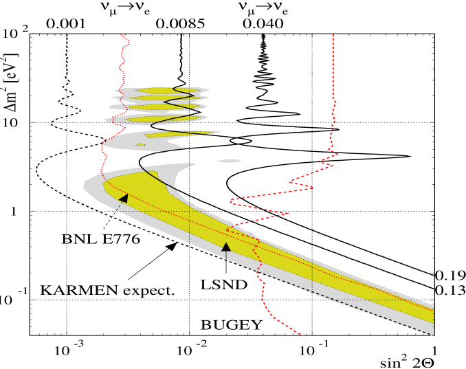
The KARMEN group also, like the LSND group, have performed two kinds of appearance experiments, and . The second one is more sensitive, since the source has no . They do not find any indication of oscillation in either experiment. They find only upper limits of conversion probabilities. The results are shown in Fig. 3, where the results of some earlier experiments are also shown, including those from a reactor experiment from the Bugey reactor in France, and a Brookhaven experiment BNL E776.
In the figures, one can see the region allowed by the LSND experiment of . As is seen, there is no disagreement between the two results at the moment. However, the KARMEN group is working on an upgrade. With this, they will probe much lower values, which are shown in the figure as well. With this upgrade, they should see positive results if the LSND results are correct. And if they don’t see anything, that will be a contradiction with the LSND results.

CHOOZ
Very recently, results have come from a reactor experiment in France [4]. The experiment is done with MeV and km. Since the source of neutrinos is a reactor, the primary beam consists of . And the experiment is of disappearance type, looking for , where can be any flavor, including unknown ones. They obtain
| (4.1) |
This is consistent with no oscillations at all. At 90% CL, they use therefore
| (4.2) |
The important thing is that, even with a rather high value for , they can probe quite small values of since is small and the path length is large. Their results are shown in Fig. 4, where results of some earlier reactor experiments have also been shown.
In addition, we have also shown the region of parameter space that can explain the atmospheric neutrino anomaly measured by the Kamiokande collaboration, provided the anomaly is caused by oscillations. The CHOOZ result has ruled out the region. This of course does not mean that either CHOOZ or Kamiokande is wrong. It means that, if the atmospheric neutrino anomaly has to be explained by neutrino oscillations, it must be because the ’s are being lost by oscillating to or to some unknown species.
5 Outlook for future experiments
Let us reiterate the statement made earlier, that in fact an oscillation experiment measures directly the parameter . So, with a given sensitivity of an experiment (i.e., given ), one can probe smaller and smaller values of if one can construct experiments with larger values of the path length and smaller values of the average energy of the neutrino beam. It would thus seem that if we can perform reactor experiments with path lengths as large as possible, we would obtain the best results.
There is however a limitation to this goal. With reactor neutrinos, first of all, one can do disappearance experiments only, and measuring the survival probability is difficult. Secondly, reactor beams are not very well directed. So, if we try to go to large path lengths, we also lose considerably in the sensitivity. One can already see it in the results of the CHOOZ experiment, which uses a path length of 1 km which is considerably higher than those of earlier reactor experiments. But they paid the price by ending up with a which is considerably higher compared to these earlier experiments. One can see this from the fact that in Fig. 4, the vertical part of the line for large occurs at much higher value of for the CHOOZ experiment compared to the earlier ones. With reactor experiments, it is hard to go much beyond in terms of path length. Nevertheless, the Kamiokande group is contemplating an experiment with neutrinos from nearby reactors, where the path lengths could well be larger than a kilometer.
Accelerator beams are however well focused and one can hope to go to hundreds of kilometers of path length with them. Various long baseline experiments are in the planning or construction stage at the moment with accelerator neutrinos. We give a brief summary of them [5].
K2K :
The distance between KEK laboratory and the Kamiokande experiment in Japan is about 235 km. There is a plan of sending a neutrino beam from KEK to Kamiokande, with an average energy of 1 GeV. At Kamiokande, they will be detected. The beam-line should be finished by 1998, and data should be expected by 1999.
Fermilab–Soudan :
The distance here is 735 km. The MINOS experiment will be installed in the Soudan mines. The project may start at the beginning of the next century.
CERN–Gran-Sasso :
The distance is 732 km. Neutrino beam from CERN can be detected at Gran Sasso. Various proposals exists for detection of the neutrinos at Gran Sasso.
6 Conclusion
Since I have started with an “Introduction”, I have to end with a “Conclusion”. There are of course some obvious concluding remarks. With more experiments, we will know things better. The important point is that at the moment, there seems to be a lot of activity in the field. With the KARMEN upgrade, the LSND results will be checked, and we are looking forward to it. The long baseline experiments will usher a new era in this field, although the results of these experiments are not expected until a few years from now.
One of the things that I want to emphasize here is that the neutrino oscillation experiments at present provide the most sensitive information about neutrino mass from all terrestrial experiments. Let us compare them briefly with other kinds of experiments described in the Introduction. The kinematic tests provide only upper bounds of neutrino masses, which is of the order of a few eV for , 170 keV for , and 24 MeV for .
Neutrinoless double beta decay process is not allowed unless lepton number symmetry is violated. The amplitude of this process depends on the factor
| (6.1) |
where is the mass of the -th neutrino eigenstate. In absence of neutrino mixing, the quantity becomes equal to the mass of the . The most stringent bounds come from the Heidelberg-Moscow experiment [6]. They use 19.2 kg of and search for the process
| (6.2) |
and set the following lower limit on the lifetime:
| (6.3) |
It is not straight forward to deduce the upper bound on from this raw experimental number. The reason is that the calculation of this rate involves nuclear matrix elements, the evaluation of which cannot be done in a manner that pleases everyone. Using various evaluation of the matrix elements, one obtains the upper bound on ranging between eV to eV. One can say that the upper limit is of the order of an eV.
Neutrino oscillation experiments, on the other hand, cannot probe the mass values directly. They can measure the mass squared differences. If, inspired by the mass patterns of the charged fermions, one assumes a hierarchy in the neutrino masses, the lowest mass value probed would be the square root of the lowest probed. With this assumption, we see the neutrino oscillation experiments are already probing mass values which are lower than an eV. With upgrades and improvements, they can go to even lower values. Fortunately, these upgrades and improvements are not day dreaming, they are things to expect in the near future.
Acknowledgments :
I thank the organizers of the conference for giving me a chance to talk, and Lincoln Wolfenstein and Sandip Pakvasa for discussions.
References
- [1] C Athanassopoulos et al (LSND collaboration): Phys. Rev. Lett. 77 (1996) 3082; Phys. Rev. C54 (1996) 2685.
- [2] C Athanassopoulos et al (LSND collaboration): nucl-ex/9709006 (submitted to Phys. Rev. Lett.); nucl-ex/9706006 (submitted to Phys. Rev. C).
- [3] K Eitel for the KARMEN collaboration: hep-ex/9706023.
- [4] M Apollonio et al: hep-ex/9711002.
- [5] For a summary, see K Zuber: hep-ph/9712378.
- [6] M Günther et al: Phys. Rev. D55 (1997) 54.