Complete next-to-leading order perturbative QCD prediction for the pion electromagnetic form factor

Abstract

We present the results of a complete leading-twist next-to-leading order (NLO) QCD analysis of the spacelike pion electromagnetic form factor at large momentum transfer $Q$. We have studied their dependence on the form of the pion distribution amplitude. For a given distribution amplitude, we have examined the sensitivity of the predictions to the choice of the renormalization and factorization scales. Theoretical uncertainty of the LO results related to the renormalization scale ambiguity has been significantly reduced by including the NLO corrections. Adopting the criteria according to which a NLO prediction is considered reliable if, both, the ratio of the NLO to LO contributions and the strong coupling constant are reasonably small, we find that reliable perturbative predictions for the pion electromagnetic form factor with all distribution amplitudes considered can already be made at a momentum transfer $Q<10$ GeV, with corrections to the LO results being typically of the order of $\sim 20\%$. To check our predictions and to discriminate between the distribution amplitudes, it is necessary to obtain experimental data extending to higher values of $Q$.

I Introduction

Exclusive processes involving large momentum transfer are among the most interesting and challenging tests of quantum chromodynamics (QCD).

The framework for analyzing such processes within the context of perturbative QCD (PQCD) has been developed by Brodsky and Lepage [1], Efremov and Radyushkin [2], and Duncan and Mueller [3] (see Ref. [4] for reviews). They have demonstrated, to all orders in perturbation theory, that exclusive amplitudes involving large momentum transfer factorize into a convolution of a process-independent and perturbatively incalculable distribution amplitude, one for each hadron involved in the amplitude, with a process-dependent and perturbatively calculable hard-scattering amplitude.

Within the framework developed in Refs. [1, 2, 3], leading-order (LO) predictions have been obtained for many exclusive processes. It is well known, however, that, unlike in QED, the LO predictions in PQCD do not have much predictive power, and that higher-order corrections are essential for many reasons. In general, they have a stabilizing effect reducing the dependence of the predictions on the schemes and scales. Therefore, to achieve a complete confrontation between theoretical predictions and experimental data, it is very important to know the size of radiative corrections to the LO predictions. The list of exclusive processes at large momentum transfer analyzed at next-to-leading order (NLO) is very short and includes only three processes: the pion electromagnetic form factor [5, 6, 7, 8, 9, 10], the pion transition form factor [10, 11, 12], and photon-photon annihilation into two flavor-nonsinglet helicity-zero mesons, $\gamma\gamma\rightarrow M\overline{M}$ ($M=\pi$, $K$) [13].

In leading twist, the pion electromagnetic form factor (the simplest exclusive quantity) can be written as

$$F_{\pi}(Q^{2})=\int_{0}^{1}dx\int_{0}^{1}dy\;{\sl\Phi}^{*}(y,\mu_{F}^{2})\;T_{H}(x,y,Q^{2},\mu_{R}^{2},\mu_{F}^{2})\;{\sl\Phi}(x,\mu_{F}^{2})\,.$$ (1)

Here ${\sl\Phi}(x,\mu_{F}^{2})$ is the pion distribution amplitude, i.e., the probability amplitude for finding the valence $q_{1}\overline{q}_{2}$ Fock state in the initial pion with the constituents carrying the longitudinal momentum $xP$ and $(1-x)P$; $T_{H}(x,y,Q^{2},\mu_{R}^{2},\mu_{F}^{2})$ is the hard-scattering amplitude, i.e., the amplitude for a parallel $q_{1}\overline{q}_{2}$ pair of the total momentum $P$ hit by a virtual photon $\gamma^{*}$ of momentum $q$ to end up as a parallel $q_{1}\overline{q}_{2}$ pair of momentum $P^{\prime}=P+q$; ${\sl\Phi}^{*}(y,\mu_{F}^{2})$ is the amplitude for the final state $q_{1}\overline{q}_{2}$ to fuse back into a pion; $Q^{2}=-q^{2}$ is the momentum transfer in the process and is supposed to be large; $\mu_{R}$ is the renormalization (or coupling constant) scale and $\mu_{F}$ is the factorization (or separation) scale at which soft and hard physics factorize.

The hard-scattering amplitude $T_{H}$ can be calculated in perturbation theory and represented as a series in the QCD running coupling constant $\alpha_{S}(\mu_{R}^{2})$. The function ${\sl\Phi}$ is intrinsically nonperturbative, but its evolution can be calculated perturbatively.

Although the PQCD approach of Refs. [1, 2, 3] undoubtedly represents an adequate and efficient tool for analyzing exclusive processes at very large momentum transfer, its applicability to these processes at experimentally accessible momentum transfer has long been debated and attracted much attention. The concern has been raised [14, 15] that, even at very large momentum transfer, important contributions to these processes can arise from nonfactorizing end-point contributions of the distribution amplitudes with $x\sim 1$. It has been shown, however, that the incorporation of the Sudakov suppression effectively eliminates these soft contributions and that the PQCD approach to the pion form factor begins to be self-consistent for a momentum transfer of about $Q^{2}>4$ GeV² [16] (see also Ref. [17]).

To obtain the complete NLO prediction for the pion form factor requires calculating NLO corrections to both the hard-scattering amplitude and the evolution kernel for the pion distribution amplitude.

The NLO predictions for the pion form factor obtained in Refs. [5, 6, 7, 8, 9] are incomplete in so far as only the NLO correction to the hard-scattering amplitude has been considered, whereas the corresponding NLO corrections to the evolution of the pion distribution amplitude have been ignored. Apart from not being complete, the results of the calculations presented in Refs. [5, 6, 7, 8, 9] do not agree with one another.

Evolution of the distribution amplitude can be obtained by solving the differential-integral evolution equation using the moment method. In order to determine the NLO corrections to the evolution of the distribution amplitude, it is necessary to calculate two-loop corrections to the evolution kernel. These have been computed by different authors and the obtained results are in agreement [18]. Because of the complicated structure of these corrections, it is possible to obtain numerically only the first few moments of the evolution kernel [19]. Using these incomplete results, the first attempt to include the NLO corrections to the evolution of the distribution amplitude in the NLO analysis of the pion form factor was obtained in Ref. [10]. It has been found that the NLO corrections to the evolution of the pion distribution amplitude as well as to the pion form factor are tiny.

Considerable progress has recently been made in understanding the NLO evolution of the pion distribution amplitude [20]. Using conformal constraints, the complete formal solution of the NLO evolution equation has been obtained. Based on this result, it has been found that, contrary to the estimates given in Ref. [10], the NLO corrections to the evolution of the distribution amplitude are rather large. It has been concluded that because of the size of the discovered corrections, and their dependence upon the input distribution amplitude, the evolution of the distribution amplitude has to be included in the NLO analysis of exclusive processes at large momentum transfer.

The purpose of this paper is to present a complete leading-twist NLO QCD analysis of the spacelike pion electromagnetic form factor at large momentum transfer.

The plan of the paper is as follows. To check and verify the results obtained in Ref. [5, 6, 7, 8, 9], in Sec. II we carefully calculate all one-loop diagrams contributing to the NLO hard-scattering amplitude for the pion form factor. We use the Feynman gauge, the dimensional regularization method, and the modified minimal-subtraction ($\overline{MS}$) scheme. Our results are in agreement with those obtained in Refs. [5] (modulo typographical errors listed in [9]) and [7]. Making use of the method introduced in Ref. [20], in Sec. III we determine NLO evolutional corrections to four available candidate pion distribution amplitudes. In Sec. IV we discuss several possible choices of the renormalization scale $\mu_{R}$ and the factorization scale $\mu_{F}$. In Sec. V we obtain complete NLO numerical predictions for the pion form factor using the four candidate pion distribution amplitudes. For a given distribution amplitude we examine the sensitivity of the predictions on the renormalization and factorization scales, $\mu_{R}$ and $\mu_{F}$, respectively. We take $\Lambda_{\overline{MS}}=0.2$ GeV for the calculation presented here. Section VI is devoted to discussions and some concluding remarks.

II NLO correction to the hard-scattering amplitude

FIG. 1.: Feynman diagrams describing the $(q_{1}\overline{q}_{2})+\gamma^{*}\rightarrow(q_{1}\overline{q}_{2})$ transition amplitude in terms of which the hard-scattering amplitude for the pion form factor is obtained.

In this section we recalculate the NLO correction to the hard-scattering amplitude for the pion form factor.

In leading twist, the hard-scattering amplitude is obtained by evaluating the $(q_{1}\overline{q}_{2})+\gamma^{*}\rightarrow(q_{1}\overline{q}_{2})$ amplitude, which is described by the Feynman diagrams in Fig. 1, with massless valence quarks collinear with parent mesons. In this figure, $uP$ and $(1-u)P$ ($vP^{\prime}$ and $(1-v)P^{\prime}$) denote the longitudinal momenta of the pion constituents before the subtraction of collinear singularities. In this evaluation, terms of order $m^{2}/Q^{2}$ are not included and, since the constituents are constrained to be collinear, terms of order $k_{\perp}^{2}/Q^{2}$ ($k_{\perp}$ is the average transverse momentum in the meson) are not taken into account either. By projecting the $q_{1}\overline{q}_{2}$ pair into a color-singlet pseudoscalar state the amplitude corresponding to any of the diagrams in Fig. 1 can be written in terms of a trace of a fermion loop.

By definition, the hard-scattering amplitude $T_{H}$ is free of collinear singularities and has a well-defined expansion in $\alpha_{S}(\mu_{R}^{2})$ of the form

$$T_{H}(x,y,Q^{2},\mu_{R}^{2},\mu_{F}^{2})=\alpha_{S}(\mu_{R}^{2})\,T_{H}^{(0)}(x,y,Q^{2})$$ (3)

$$\quad\qquad\times\;\left[1+\frac{\alpha_{S}(\mu_{R}^{2})}{\pi}\,T_{H}^{(1)}(x,y,\mu_{R}^{2}/Q^{2},\mu_{F}^{2}/Q^{2})+\cdots\right]\,,$$

where

$$\alpha_{S}(\mu_{R}^{2})=\frac{4\pi}{\beta_{0}\ln(\mu_{R}^{2}/\Lambda_{QCD}^{2})}\,,$$ (4)

and

$$\beta_{0}=11-\frac{2}{3}n_{f}\,,$$ (5)

with $n_{f}$ being the effective number of quark flavors and $\Lambda_{QCD}$ is the fundamental QCD parameter.

FIG. 2.: Lowest-order Feynman diagrams contributing to the $(q_{1}\overline{q}_{2})+\gamma^{*}\rightarrow(q_{1}\overline{q}_{2})$ amplitude.

In the LO approximation (Born approximation) there are only four Feynman diagrams contributing to the $(q_{1}\overline{q}_{2})+\gamma^{*}\rightarrow(q_{1}\overline{q}_{2})$ transition amplitude. They are shown in Fig. 2. Evaluating these diagrams, one finds that the LO hard-scattering amplitude is given by

$$T_{H}^{(0)}(x,y,Q^{2})=\frac{4}{3}\frac{16\pi}{Q^{2}(1-x)(1-y)}\,.$$ (6)

To obtain this result, it is necessary to evaluate only one of the four diagrams. Namely, knowing the contribution of diagram $A$, the contribution of diagrams $B$, $C$, and $D$ can be obtained by making use of the isospin symmetry and time-reversal symmetry. In the leading-twist approximation, the isospin symmetry is exact. A consequence of this is that the contributions of diagrams $A$ and $B$ are related to the contributions of $C$ and $D$, respectively. On the other hand, diagrams $A$ and $C$ are by time-reversal symmetry related to diagrams $B$ and $D$, respectively.

At NLO there are altogether 62 one-loop Feynman diagrams contributing to the $(q_{1}\overline{q}_{2})+\gamma^{*}\rightarrow(q_{1}\overline{q}_{2})$ amplitude. They can be generated by inserting an internal gluon line into the leading-order diagrams of Fig. 2. Use of the above mentioned symmetries (isospin and time-reversal) cuts the number of independent one-loop diagrams to be evaluated from 62 to 17. They are all generated from the LO diagram $A$. We use the notation where $Aij$ is the diagram obtained from diagram $A$ by inserting the gluon line connecting the lines $i$ and $j$, where $i,j=1,2,\cdots,6$. They are shown in Fig. 3 with the exception of $A33$, $A55$, and $A66$, which give obviously the same contribution as $A11$. These diagrams contain ultraviolet (UV) singularities and, owing to the fact that initial- and final-state quarks are massless and onshell, they also contain both infrared (IR) and collinear singularities. We use dimensional regularization in $D=4-2\epsilon$ dimensions to regularize all three types of singularities, distinguishing the poles $1/\epsilon$ by the subscripts UV and IR ($D=4-2\epsilon_{UV}=4+2\epsilon_{IR}$). Soft singularity is always accompanied by two collinear singularities and, consequently, when dimensionally regularized, leads to the double pole $1/\epsilon_{IR}^{2}$.

FIG. 3.: Distinct one-loop Feynman diagrams contributing to the $(q_{1}\overline{q}_{2})+\gamma^{*}\rightarrow(q_{1}\overline{q}_{2})$ amplitude. The total number of diagrams is 62.

Before the subtraction of divergences has been performed, the pion form factor convolution formula reads

$$F_{\pi}(Q^{2})=\int_{0}^{1}du\int_{0}^{1}dv\;{\sl\Phi}^{*}(v)\;\Delta(u,v,\mu_{UV}^{2}/Q^{2},\mu_{IR}^{2}/Q^{2})\;{\sl\Phi}(u)\,,$$ (7)

where $\Delta(u,v,\mu_{UV}^{2}/Q^{2},\mu_{IR}^{2}/Q^{2})$ denotes the amplitude for the $(q_{1}\overline{q}_{2})+\gamma^{*}\rightarrow(q_{1}\overline{q}_{2})$ quark subprocess. This amplitude has the expansion of the form

$$\Delta(u,v,\mu_{UV}^{2}/Q^{2},\mu_{IR}^{2}/Q^{2})=\alpha_{S}\,\Delta^{(0)}(u,v,Q^{2})+\frac{\alpha_{S}^{2}}{\pi}\Delta^{(1)}(u,v,\mu_{UV}^{2}/Q^{2},\mu_{IR}^{2}/Q^{2})+...\,,$$ (8)

where

$$\Delta^{(0)}(u,v,Q^{2})=(1-\epsilon)\,T_{H}^{(0)}(u,v,Q^{2})\,.$$ (9)

The contributions of the individual diagrams to $\Delta^{(1)}(u,v,\mu_{UV}^{2}/Q^{2},\mu_{IR}^{2}/Q^{2})$, with the overall factor $T_{H}^{(0)}(u,v,Q^{2})$ of Eq. (6) extracted, are listed in Table I. We have used the following notation:

$$\overline{u}\, = 1-u,\;\overline{v}\,=1-v\,,$$ (10)

$$\eta_{UV} = \frac{1}{\epsilon_{UV}}-\gamma-\ln\frac{Q^{2}}{4\pi\mu_{UV}^{2}}=\frac{1}{\hat{\epsilon}_{UV}}+\ln\frac{\mu_{UV}^{2}}{Q^{2}}\,,$$ (11)

$$\eta_{IR} = \frac{1}{\epsilon_{IR}}+\gamma+\ln\frac{Q^{2}}{4\pi\mu_{IR}^{2}}=\frac{1}{\hat{\epsilon}_{IR}}-\ln\frac{\mu_{IR}^{2}}{Q^{2}}\,,$$ (12)

$$\tilde{\eta}_{IR} = \frac{1}{\epsilon_{IR}^{2}}+\frac{1}{\epsilon_{IR}}\left(\gamma+\ln\frac{Q^{2}}{4\pi\mu_{IR}^{2}}\right)+\frac{1}{2}\left(\gamma^{2}-\frac{\pi^{2}}{6}\right)$$ (14)

$$+\gamma\ln\frac{Q^{2}}{4\pi\mu_{IR}^{2}}+\frac{1}{2}\ln^{2}\frac{Q^{2}}{4\pi\mu_{IR}^{2}}\,,$$

$$\frac{1}{\hat{\epsilon}_{UV}} = \frac{1}{\epsilon_{UV}}-\gamma+\ln(4\pi)\,,$$ (15)

$$\frac{1}{\hat{\epsilon}_{IR}} = \frac{1}{\epsilon_{IR}}+\gamma-\ln(4\pi)\,.$$ (16)

TABLE I.: Contributions to $\Delta^{(1)}(u,v,\mu_{R}^{2}/Q^{2},\mu_{F}^{2}/Q^{2})$ (defined by (8)) of Feynman diagrams shown in Fig. 3 .

A11	$\displaystyle-\frac{1}{12}(\eta_{UV}+\eta_{IR})$
A22	$\displaystyle-\frac{1}{6}(\eta_{UV}-\ln\overline{v}\,)$
A44	$\displaystyle\frac{1}{8}\left[\left(5-\frac{2}{3}n_{f}\right)(\eta_{UV}-\ln(\overline{u}\,\overline{v}\,))+\frac{16}{3}-\frac{4}{9}n_{f}\right]$
A23	$\displaystyle\frac{1}{6}\left(\eta_{UV}+\frac{1+\overline{v}\,}{v}\ln\overline{v}\,\right)$
A12	$\displaystyle-\frac{1}{48}\left[\eta_{UV}+2\eta_{IR}\left(1+\frac{\overline{u}\,}{u}\ln{\overline{u}\,}\right)-3-\frac{\overline{u}\,}{u}\ln{\overline{u}\,}+\ln{\overline{v}\,}+\frac{\overline{u}\,}{u}\ln^{2}\overline{u}\,+2\frac{\overline{u}\,}{u}\ln{\overline{u}\,}\ln{\overline{v}\,}\right]$
A56	$\displaystyle-\frac{1}{48}[\eta_{UV}+2\eta_{IR}(1-\ln(\overline{u}\,\overline{v}\,))-2\tilde{\eta}_{IR}-5+\ln(\overline{u}\,\overline{v}\,)-\ln^{2}\overline{u}\,-\ln^{2}\overline{v}\,-2\ln\overline{u}\,\ln\overline{v}\,]$
A14	$\displaystyle\frac{3}{16}\left[3\eta_{UV}+2\eta_{IR}\left(1+\frac{\ln{\overline{u}\,}}{u}\right)+1+\ln\frac{\overline{u}\,}{\overline{v}\,}+\frac{\ln^{2}\overline{u}\,}{u}+2\frac{\ln\overline{u}\,\ln\overline{v}\,}{u}\right]$
A45	$\displaystyle\frac{3}{16}[3\eta_{UV}+4\eta_{IR}-1+\ln(\overline{u}\,\overline{v}\,)]$
A15	$\displaystyle-\frac{1}{3}\frac{\overline{u}\,}{u}\left[\eta_{IR}\ln\overline{u}\,+\ln\overline{u}\,+\frac{1}{2}\ln^{2}\overline{u}\,+\ln\overline{u}\,\ln\overline{v}\,\right]$
A16	$\displaystyle-\frac{1}{24}\left[\tilde{\eta}_{IR}+\eta_{IR}\left(1+\frac{\ln\overline{u}\,}{u}+2\ln u+\ln\overline{v}\,\right)+\frac{\ln\overline{u}\,}{u}+2\ln u+\ln\overline{v}\,+\frac{1}{2}\frac{\ln^{2}\overline{u}\,}{u}+\ln^{2}u\right.$
	$\displaystyle\left.+\frac{1}{2}\ln^{2}\overline{v}\,+\frac{\ln\overline{u}\,\ln\overline{v}\,}{u}+2\ln u\ln\overline{v}\,\right]$
A34	$\displaystyle\frac{3}{8}\left[\eta_{IR}\left(2+\frac{\ln\overline{u}\,}{u}+\frac{\ln\overline{v}\,}{v}\right)-2+\ln\overline{u}\,+\ln\overline{v}\,+\frac{\overline{u}\,+\overline{v}\,}{uv}\ln\overline{u}\,\ln\overline{v}\,+\frac{1}{2u}\ln^{2}\overline{u}\,+\frac{1}{2v}\ln^{2}\overline{v}\,\right]$
A13	$\displaystyle\frac{1}{24}\left\{\tilde{\eta}_{IR}+\eta_{IR}\left(\frac{\overline{u}\,}{u}\ln\overline{u}\,+\ln u+\ln v\right)+1\right.$
	$\displaystyle\left.+\frac{\overline{u}\,}{2u}\ln^{2}\overline{u}\,+\frac{1}{2}\ln^{2}u+\frac{1}{2}\ln^{2}v+\ln u\ln v+\frac{\overline{u}\,}{u}\ln\overline{u}\,\ln\overline{v}\,\right.$
	$\displaystyle\left.-\frac{1}{2(u-v)^{2}}\left[4\overline{u}\,^{2}u\mbox{H}(u,\overline{v}\,)+(4u-5u^{2}+v^{2})(\ln u+\ln v)\right.\right.$
	$\displaystyle\left.\left.+(6u-5u^{2}-2v+v^{2})\overline{u}\,\frac{\ln\overline{u}\,}{u}+(2u-4u^{2}+2v-4uv+5u^{2}v-v^{3})\frac{\ln\overline{v}\,}{v}\right]\right\}$
A36	$\displaystyle-\frac{1}{3}\left[\eta_{IR}\left(\frac{\overline{u}\,}{u}\ln{\overline{u}\,}+\frac{\overline{v}\,}{v}\ln\overline{v}\,\right)+\frac{\overline{u}\,}{u}\ln\overline{u}\,+\frac{\overline{v}\,}{v}\ln\overline{v}\,+\frac{\overline{u}\,}{2u}\ln^{2}\overline{u}\,+\frac{\overline{v}\,}{2v}\ln^{2}\overline{v}\,+\frac{\overline{u}\,+\overline{v}\,}{uv}\ln\overline{u}\,\ln\overline{v}\,\right]$
A35	$\displaystyle-\frac{1}{24}\left[2\tilde{\eta}_{IR}+\eta_{IR}\left(2+\frac{1+u}{u}\ln\overline{u}\,+\frac{1+v}{v}\ln\overline{v}\,\right)-2(1-u-v)\mbox{H}(u,v)+\frac{1+u}{u}\ln\overline{u}\,\right.$
	$\displaystyle\left.+\frac{1+v}{v}\ln\overline{v}\,+\frac{1+u}{2u}\ln^{2}\overline{u}\,+\frac{1+v}{2v}\ln^{2}\overline{v}\,+\frac{\overline{u}\,+\overline{v}\,}{uv}\ln\overline{u}\,\ln\overline{v}\,\right]$

The function $\mbox{H}(u,v)$ appearing in Table I is given by the expression

$$\mbox{H}(u,v) = \frac{1}{1-u-v}\left[\mbox{Li}_{2}\left(\frac{\overline{v}\,}{u}\right)+\mbox{Li}_{2}\left(\frac{\overline{u}\,}{v}\right)+\mbox{Li}_{2}\left(\frac{uv}{\overline{u}\,\overline{v}\,}\right)\right.$$ (18)

$$\left.-\mbox{Li}_{2}\left(\frac{u}{\overline{v}\,}\right)-\mbox{Li}_{2}\left(\frac{v}{\overline{u}\,}\right)-\mbox{Li}_{2}\left(\frac{\overline{u}\,\overline{v}\,}{uv}\right)\right]\,,$$

where $\mbox{Li}_{2}(u)$ is the Spence function defined as

$$\mbox{Li}_{2}(u)=-\int_{0}^{u}\frac{\ln(1-t)}{t}dt\,.$$ (19)

Adding up the contributions of all diagrams, we find that the NLO contribution to the $(q_{1}\overline{q}_{2})+\gamma^{*}\rightarrow(q_{1}\overline{q}_{2})$ amplitude, given in (8), can be written in the form

$$\Delta^{(1)}(u,v,\mu_{UV}^{2}/Q^{2},\mu_{IR}^{2}/Q^{2})$$ (20)

$$\quad= T_{H}^{(0)}(u,v,Q^{2})\,\left[C_{UV}\frac{1}{\hat{\epsilon}_{UV}}+C_{IR}(u,v)\frac{1}{\hat{\epsilon}_{IR}}\right.$$ (21)

$$\left.+\widetilde{f}_{UV}(u,v,\mu_{UV}^{2}/Q^{2})+\widetilde{f}_{IR}(u,v,\mu_{IR}^{2}/Q^{2})+\widetilde{f}_{C}(u,v)\right]\,,$$ (22)

where

$$C_{UV} = \frac{1}{4}\beta_{0}\,,$$ (24)

$$C_{IR}(u,v) = \frac{2}{3}\left[3+\ln(\overline{u}\,\overline{v}\,)\right]\,,$$ (25)

and

$$\widetilde{f}_{UV}(u,v,\mu_{UV}^{2}/Q^{2}) = C_{UV}\left[\frac{2}{3}-\ln(\overline{u}\,\overline{v}\,)+\ln\frac{\mu_{UV}^{2}}{Q^{2}}\right]\,,$$ (27)

$$\widetilde{f}_{IR}(u,v,\mu_{IR}^{2}/Q^{2}) = C_{IR}(u,v)\left[\frac{1}{2}\ln(\overline{u}\,\overline{v}\,)-\ln\frac{\mu_{IR}^{2}}{Q^{2}}\right]\,,$$ (28)

$$\widetilde{f}_{C}(u,v) = \frac{1}{12}\left[-10+20\ln(\overline{u}\,\overline{v}\,)+\ln u\ln v\right.$$ (31)

$$\left.+\ln\overline{u}\,\ln\overline{v}\,-\ln u\ln\overline{v}\,-\ln\overline{u}\,\ln v\right.$$

$$\left.+(1-u-v)\mbox{H}(u,v)+\mbox{R}(u,v)\right]\,.$$

The function $\mbox{R}(u,v)$ is defined as

$$\mbox{R}(u,v) = \frac{1}{(u-v)^{2}}\left[(2uv-u-v)(\ln u+\ln v)\right.$$ (35)

$$\left.+(-2uv^{2}-2v^{2}+10uv-2v-4u^{2})\frac{\ln\overline{v}\,}{v}\right.$$

$$\left.+(-2vu^{2}-2u^{2}+10uv-2u-4v^{2})\frac{\ln\overline{u}\,}{u}\right.$$

$$\left.-(v\overline{v}\,^{2}+u\overline{u}\,^{2})\mbox{H}(u,\overline{v}\,)\right]\,.$$

The contributions of the individual diagrams listed in Table I are in agreement with those obtained in Ref. [5] (up to some typographical errors listed in [9]). Correspondence between our results and those of Ref. [5] is established by multiplying the latter by $(P+P^{\prime})^{\mu}/Q^{2}$.

It is easily seen from Eqs. (22-35) that in summing up the contributions of all diagrams to the exclusive $(q_{1}\overline{q}_{2})+\gamma^{*}\rightarrow(q_{1}\overline{q}_{2})$ amplitude, the originally present soft singularities (double $1/\epsilon_{IR}^{2}$ poles) cancel out, as required. The final result for the amplitude contains $1/\epsilon_{UV}$ and only simple $1/\epsilon_{IR}$ poles.

We now proceed to treat these poles. When doing this, one has to exercise some care, since the subtractions have to be performed in such a way that the universality of the distribution amplitude as well as the universality of the coupling constant are simultaneously preserved.

The IR poles in (22), related to collinear singularities, are such that they can be absorbed into the pion distribution amplitude. The universality of the distribution amplitude requires that the poles $1/\epsilon_{IR}$ should be absorbed by some universal renormalization factor [8, 21]. The regularization-dependent terms represent “soft” effects and therefore we absorb them into the distribution amplitude along with the singularities. A crucial observation is that the structure of the collinearly divergent terms in (22) is such that one can write

$$V_{1}(v,y)\otimes T_{H}^{(0)}(x,y,Q^{2})\otimes\delta(x-u)+\delta(v-y)\otimes T_{H}^{(0)}(x,y,Q^{2})\otimes V_{1}(x,u)$$ (36)

$$\qquad\qquad=C_{IR}(u,v)T_{H}^{(0)}(u,v,Q^{2})\,,$$ (37)

where the function $V_{1}(x,u)$ is the one-loop evolution kernel for the pion distribution amplitude (see the corresponding expression in, for example, [5] or [22]), while $\otimes$ denotes the convolution symbol defined as

$$A(z)\otimes B(z)=\int_{0}^{1}dz\,A(z)\,B(z)\>.$$ (38)

Based on Eq. (37), the NLO expression for the $(q_{1}\overline{q}_{2})+\gamma^{*}\rightarrow(q_{1}\overline{q}_{2})$ amplitude, given by (8), (22-35), can be written in a factorized form

$$\alpha_{S}\,\Delta^{(0)}(u,v,Q^{2};\epsilon_{IR})+\frac{\alpha_{S}^{2}}{\pi}\Delta^{(1)}(u,v,\mu_{IR}^{2}/Q^{2};1/\epsilon_{IR})$$ (39)

$$\quad= \left[\delta(v-y)+\frac{\alpha_{S}}{\pi}V_{1}(v,y)\left(\frac{1}{\hat{\epsilon}_{IR}}+\ln\frac{\mu_{F}^{2}}{\mu_{IR}^{2}}\right)\right]$$ (40)

$$\otimes\left\{\alpha_{S}T_{H}^{(0)}(x,y,Q^{2})\left[(1-\epsilon)+\frac{\alpha_{S}}{\pi}\widehat{T}_{H}^{(1)}(x,y,\mu_{F}^{2}/Q^{2};\epsilon_{IR})\right]\right\}$$ (41)

$$\otimes\left[\delta(x-u)+\frac{\alpha_{S}}{\pi}V_{1}(x,u)\left(\frac{1}{\hat{\epsilon}_{IR}}+\ln\frac{\mu_{F}^{2}}{\mu_{IR}^{2}}\right)\right]\,.$$ (42)

Formula (42) shows the essence of the procedure for the separation of collinear divergences, which is schematically represented in Fig. 4. The procedure consists in summing the effects of collinear divergences contained in the shaded rectangular region in Fig. 4, as a result of which the outside quark (antiquark) with momentum $uP$ ($\overline{u}\,P$) ends up on the inside quark (antiquark) of momentum $xP$ ($\overline{x}\,P$).

FIG. 4.: Pictorial representation of the procedure for absorbing the collinear divergences into the pion distribution amplitude $\Phi(x,\mu_{F}^{2})$.

As for the UV poles, we renormalize them using the modified minimal-subtraction ($\overline{\mbox{MS}}$) scheme. This is carried out by stating that $\alpha_{S}$ appearing in (8) is the bare unrenormalized coupling related to the renormalized physical coupling $\alpha_{\overline{MS}}(\mu_{R}^{2})$ by

$$\alpha_{S}=\alpha_{\overline{MS}}(\mu_{R}^{2})\left[1-\frac{\alpha_{\overline{MS}}(\mu_{R}^{2})}{\pi}\frac{\beta_{0}}{4}\left(\frac{1}{\hat{\epsilon}_{UV}}-\ln\frac{\mu_{R}^{2}}{\mu_{UV}^{2}}\right)\right]\,.$$ (43)

It is important to note that the $\epsilon\rightarrow 0$ limit can be taken only after the separation of collinear divergences and UV renormalization have been performed (taking the $\epsilon\rightarrow 0$ limit in $\Delta^{(0)}$ before the subtraction of IR and UV singularities is equivalent to choosing a factorization scheme that does not respect the universality of the distribution amplitude (see [8]) and the renormalization scheme in which the running coupling constant is not universal). As a result, we obtain the following expression for the NLO hard-scattering amplitude for the pion form factor:

$$T_{H}(x,y,Q^{2},\mu_{R}^{2},\mu_{F}^{2})=\alpha_{\overline{MS}}(\mu_{R}^{2})\,T_{H}^{(0)}(x,y,Q^{2})$$ (45)

$$\qquad\qquad\times\;\left[1+\frac{\alpha_{\overline{MS}}(\mu_{R}^{2})}{\pi}\,T_{H}^{(1)}(x,y,\mu_{R}^{2}/Q^{2},\mu_{F}^{2}/Q^{2})\right]\,,$$

where

$$T_{H}^{(1)}(x,y,\mu_{R}^{2}/Q^{2},\mu_{F}^{2}/Q^{2})$$ (46)

$$= f_{UV}(x,y,\mu_{R}^{2}/Q^{2})+f_{IR}(x,y,\mu_{F}^{2}/Q^{2})+f_{C}(x,y)\,,$$ (47)

and

$$f_{UV}(x,y,\mu_{R}^{2}/Q^{2}) = \widetilde{f}_{UV}(x,y,\mu_{R}^{2}/Q^{2})+C_{UV}$$ (49)

$$= \frac{1}{4}\beta_{0}\left[\frac{5}{3}-\ln(\overline{x}\,\overline{y}\,)+\ln\frac{\mu_{R}^{2}}{Q^{2}}\right]\,,$$ (50)

$$f_{IR}(x,y,\mu_{F}^{2}/Q^{2}) = \widetilde{f}_{IR}(x,y,\mu_{F}^{2}/Q^{2})$$ (51)

$$= \frac{2}{3}\left[3+\ln(\overline{x}\,\overline{y}\,)\right]\left[\frac{1}{2}\ln(\overline{x}\,\overline{y}\,)-\ln\frac{\mu_{F}^{2}}{Q^{2}}\right]\,,$$ (52)

$$f_{C}(x,y) = \widetilde{f}_{C}(x,y)-C_{IR}(x,y)$$ (53)

$$= \frac{1}{12}\left[-34+12\ln(\overline{x}\,\overline{y}\,)+\ln x\ln y\right.$$ (56)

$$\left.+\ln\overline{x}\,\ln\overline{y}\,-\ln x\ln\overline{y}\,-\ln\overline{x}\,\ln y\right.$$

$$\left.+(1-x-y)\mbox{H}(x,y)+\mbox{R}(x,y)\right]\,.$$

A few comments on the previously performed calculations are in order. Our final expression for the hard-scattering amplitude $T_{H}$ is in agreement with Ref. [7]. The calculation of [5] contains a few typographical errors in the diagram-by-diagram listing as well as in the final expression (which are all listed in [9]). Apart from this, the results from Ref. [5] agree with ours. In Refs. [6, 8] the contribution of the diagrams with propagator corrections on external quark lines were not taken into account. Also, in Ref. [6] the subtraction of collinear singularities was performed in a way that is not consistent with the universality of the distribution amplitude (see the discussion in Ref. [8]). Finally, a thorough analysis of the results of Refs. [5, 6, 7] was performed in Ref. [9], but in obtaining the final expression for the hard-scattering amplitude $T_{H}$, collinear and UV divergences were subtracted in a way that is not consistent with the universality of both the distribution amplitude and the running coupling constant.

III Evolutional corrections to the pion distribution amplitude

The pion distribution amplitude ${\sl\Phi}(x,\mu_{F}^{2})$, controlling exclusive pion processes at large momentum transfer, is the basic valence wave function of the pion. Its form is not yet accurately known. It has been shown, however, that the leptonic decay $\pi^{+}\rightarrow\mu^{+}\nu_{\mu}$ imposes on ${\sl\Phi}(x,\mu_{F}^{2})$ a constraint of the form

$$\int_{0}^{1}dx\,{\sl\Phi}(x,\mu_{F}^{2})=\frac{f_{\pi}}{2\sqrt{2n_{C}}}\,.$$ (57)

Given the form of ${\sl\Phi}(x,\mu_{F}^{2})$, this relation normalizes it for any $\mu_{F}^{2}$. In (57), $f_{\pi}=0.131$ GeV is the pion decay constant and $n_{C}$($=3$) is the number of QCD colors.

Instead of using ${\sl\Phi}(x,\mu_{F}^{2})$ satisfying (57), one usually introduces the distribution amplitude $\phi(x,\mu_{F}^{2})$ normalized to unity,

$$\int_{0}^{1}dx\,\phi(x,\mu_{F}^{2})=1\,,$$ (58)

and related to ${\sl\Phi}(x,\mu_{F}^{2})$ by

$${\sl\Phi}(x,\mu_{F}^{2})=\frac{f_{\pi}}{2\sqrt{2n_{C}}}\phi(x,\mu_{F}^{2})\,.$$ (59)

Although intrinsically nonperturbative, the pion distribution amplitude $\phi(x,\mu_{F}^{2})$ satisfies an evolution equation of the form

$$\mu_{F}^{2}\frac{\partial}{\partial\mu_{F}^{2}}\phi(x,\mu_{F}^{2})=\int_{0}^{1}du\;V(x,u,\alpha_{S}(\mu_{F}^{2}))\;\phi(u,\mu_{F}^{2})\,,$$ (60)

in which the evolution kernel is calculable in perturbation theory:

$$V(x,u,\alpha_{S}(\mu_{F}^{2}))$$ (62)

$$\quad=\frac{\alpha_{S}(\mu_{F}^{2})}{\pi}\,V_{1}(x,u)+\left(\frac{\alpha_{S}(\mu_{F}^{2})}{\pi}\right)^{2}V_{2}(x,u)+\cdots$$

and has been computed in the one- and two-loop approximations using dimensional regularization and the $\overline{MS}$ scheme.

If the distribution amplitude $\phi(x,\mu_{0}^{2})$ can be calculated at an initial momentum scale $\mu_{0}^{2}$ using QCD sum rules [23] or lattice gauge theory [24], then the differential-integral evolution equation (60) can be integrated using the moment method to give $\phi(x,\mu_{F}^{2})$ at any momentum scale $\mu_{F}^{2}>\mu_{0}^{2}$.

Because of the complicated structure of the two-loop contribution to the evolutional kernel $V_{2}(x,y)$, only the first few moments of the evolutional kernel have been computed numerically.

Recently, based on the conformal spin expansion and the conformal consistency relation, the analytical result for the evolution of the flavor-nonsinglet meson distribution amplitude has been determined [20].

To the NLO approximation, this, rather complicated solution has the form

$$\phi(x,\mu_{F}^{2})=\phi^{LO}(x,\mu_{F}^{2})+\frac{\alpha_{S}(\mu_{F}^{2})}{\pi}\,\phi^{NLO}(x,\mu_{F}^{2})\,,$$ (64)

where

$$\phi^{LO}(x,\mu_{F}^{2}) = x\,(1-x)\sum_{n=0}^{\infty}{}^{\prime}\>C_{n}^{3/2}(2x-1)\;\frac{4(2n+3)}{(n+1)(n+2)}\,$$ (66)

$$\times\,\left(\frac{\alpha_{S}(\mu_{0}^{2})}{\alpha_{S}(\mu_{F}^{2})}\right)^{\gamma_{n}^{(0)}/\beta_{0}}\,\int_{0}^{1}dy\,C_{n}^{3/2}(2y-1)\,\phi(y,\mu_{0}^{2})\,,$$

and

$$\phi^{NLO}(x,\mu_{F}^{2}) = x\,(1-x)\,\sum_{n=0}^{\infty}{}^{\prime}\>\left(\frac{\alpha_{S}(\mu_{0}^{2})}{\alpha_{S}(\mu_{F}^{2})}\right)^{\gamma_{n}^{(0)}/\beta_{0}}\,\int_{0}^{1}dy\,C_{n}^{3/2}(2y-1)\,\phi(y,\mu_{0}^{2})$$ (69)

$$\left[C_{n}^{3/2}(2x-1)\frac{(2n+3)}{(n+1)(n+2)}\left(1-\frac{\alpha_{S}(\mu_{0}^{2})}{\alpha_{S}(\mu_{F}^{2})}\right)\,\left(\frac{\gamma_{n}^{(1)}}{2\beta_{0}}+\frac{\beta_{1}}{\beta_{0}^{2}}\gamma_{n}^{(0)}\right)\right.$$

$$\left.+\sum_{k=n+2}^{\infty}{}^{\prime}\>C_{k}^{3/2}(2x-1)\frac{2(2k+3)}{(k+1)(k+2)}S_{kn}(\mu_{F}^{2})\,C_{kn}^{(1)}\right]\,,$$

with abbreviations

$$S_{kn}(\mu_{F}^{2}) = \frac{\gamma_{k}^{(0)}-\gamma_{n}^{(0)}}{\gamma_{k}^{(0)}-\gamma_{n}^{(0)}+\beta_{0}}\left[1-\left(\frac{\alpha_{S}(\mu_{0}^{2})}{\alpha_{S}(\mu_{F}^{2})}\right)^{1+(\gamma_{k}^{(0)}-\gamma_{n}^{(0)})/\beta_{0}}\right]\,,$$ (70)

$$C_{kn}^{(1)} = (2n+3)\left[\frac{\gamma_{n}^{(0)}-\beta_{0}+4C_{F}A_{kn}}{(k-n)(k+n+3)}+\frac{2C_{F}(A_{kn}-\psi(k+2)+\psi(1))}{(n+1)(n+2)}\right]\,,$$ (71)

$$A_{kn} = \psi(\frac{k+n+4}{2})-\psi(\frac{k-n}{2})+2\psi(k-n)-\psi(k+2)-\psi(1)\,,$$ (73)

and $\sum{}^{\prime}$ denoting the sum running only over even $n$, while $C_{n}^{3/2}(z)$ are Gegenbauer polynomials of order $3/2$ and $C_{F}=4/3$.

In Eqs. (66–LABEL:eq:Ckn1), $\gamma_{n}^{(0)}$ are the usual anomalous dimensions:

$$\gamma_{n}^{(0)}=C_{F}\left[3+\frac{2}{(n+1)(n+2)}-4\sum_{i=1}^{n+1}\frac{1}{i}\right]\,,$$ (74)

while $\beta_{0}$ and $\beta_{1}$ are the first two terms in the expansion of the QCD $\beta$–function, with $\beta_{0}$ given by (5), and

$$\beta_{1}=102-\frac{38}{3}n_{f}\,.$$ (75)

The function $\psi(z)$ appearing in (LABEL:eq:Ckn1) and (73) is defined as

$$\psi(z)=\frac{d}{dz}(\ln\Gamma(z)).$$ (76)

For $n_{f}=3$ and for the values of $n$ we are interested in, we have taken the values of the anomalous dimension $\gamma_{n}^{(1)}$ from [25, 26]:

$$\gamma_{0}^{(1)}=0\,,\qquad\gamma_{2}^{(1)}=111.03\,,\qquad\gamma_{4}^{(1)}=150.28\,.$$ (77)

To proceed, we expand the distribution amplitude $\phi(x,\mu_{0}^{2})$ in terms of the Gegenbauer polynomials $C_{n}^{3/2}(2x-1)$ (the eigenfunctions of the LO evolution equation)

$$\phi(x)=\phi(x,\mu_{0}^{2})=6x(1-x)\,\sum_{n=0}^{\infty}{}^{\prime}B_{n}\>C_{n}^{3/2}(2x-1)\,.$$ (78)

Owing to the orthogonality of the Gegenbauer polynomials, the expansion coefficients $B_{n}$ are given by

$$B_{n}=\frac{1}{6}\,\frac{4(2n+3)}{(n+1)(n+2)}\,\int_{0}^{1}dx\,C_{n}^{3/2}(2x-1)\,\phi(x)\,$$ (79)

and the normalization condition (58) then implies $B_{0}=1$. Substituting (78) into (66) gives

$$\phi^{LO}(x,\mu_{F}^{2})=6x(1-x)\,\sum_{n=0}^{\infty}{}^{\prime}B_{n}^{LO}(\mu_{F}^{2})\>C_{n}^{3/2}(2x-1)\,,$$ (80)

where

$$B_{n}^{LO}(\mu_{F}^{2})=B_{n}\left(\frac{\alpha_{S}(\mu_{0}^{2})}{\alpha_{S}(\mu_{F}^{2})}\right)^{\gamma_{n}^{(0)}/\beta_{0}}\,,$$ (81)

so that, obviously, $B_{0}^{LO}=1$. Next, by taking (78) into account (69) becomes

$$\phi^{NLO}(x,\mu_{F}^{2})=6x(1-x)\,\sum_{k=2}^{\infty}{}^{\prime}B_{k}^{NLO}(\mu_{F}^{2})\;C_{k}^{3/2}(2x-1)\,,$$ (82)

where

$$B_{k}^{NLO}(\mu_{F}^{2})=B_{k}^{LO}(\mu_{F}^{2})P_{k}(\mu_{F}^{2})+\sum_{n=0}^{k-2}{}^{\prime}B_{n}^{LO}(\mu_{F}^{2})Q_{kn}(\mu_{F}^{2})\,,$$ (83)

and

$$P_{k}(\mu_{F}^{2}) = \frac{1}{4}\,\left(\frac{\gamma_{k}^{(1)}}{2\beta_{0}}+\frac{\beta_{1}}{\beta_{0}^{2}}\gamma_{k}^{(0)}\right)\,\left(1-\frac{\alpha_{S}(\mu_{0}^{2})}{\alpha_{S}(\mu_{F}^{2})}\right)\,,$$ (84)

$$Q_{kn}(\mu_{F}^{2}) = \frac{(2k+3)}{(k+1)(k+2)}\,\frac{(n+2)(n+1)}{2(2n+3)}\,C_{kn}^{(1)}\,S_{kn}(\mu_{F}^{2})\,.$$ (85)

For the purpose of our calculation, we use the following four candidate distribution amplitudes (shown in Fig. 5) as nonperturbative inputs at the reference momentum scale $\mu_{0}^{2}=(0.5$ GeV$)^{2}$:

$$\phi_{as}(x) \equiv \phi_{as}(x,\mu_{0}^{2})\,=\,6x(1-x)\,,$$ (87)

$$\phi_{CZ}(x) \equiv \phi_{CZ}(x,\mu_{0}^{2})\,=\,6x(1-x)\left[5(2x-1)^{2}\right]\,,$$ (88)

$$\phi_{P2}(x) \equiv \phi_{P2}(x,\mu_{0}^{2})=6x(1-x)\left[-0.1821+5.91(2x-1)^{2}\right]\,,$$ (89)

$$\phi_{P3}(x) \equiv \phi_{P3}(x,\mu_{0}^{2})=6x(1-x)\left[0.6016-4.659(2x-1)^{2}+15.52(2x-1)^{4}\right]\,.$$ (90)

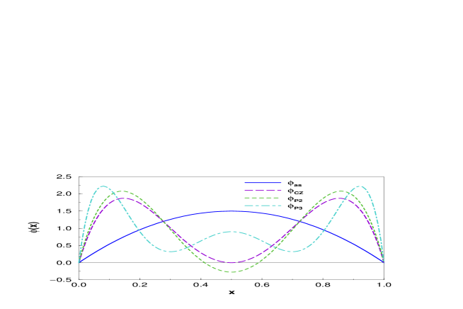
FIG. 5.: The four candidate pion distribution amplitudes defined by Eqs. (III), chosen as nonperturbative inputs at the reference scale $\mu_{0}^{2}=(0.5$GeV$)^{2}$.

Here $\phi_{as}(x)$ is the asymptotic distribution amplitude and represents the solution of the evolution equation (60) for $\mu_{F}^{2}\rightarrow\infty$. The double-hump-shaped distribution amplitudes $\phi_{CZ}(x)$ and $\phi_{P2}(x)$ and the three-hump-shaped distribution amplitude $\phi_{P3}(x)$ have been obtained using the method of QCD sum rules [23, 27]. As Fig. 5 shows, these distribution amplitudes, unlike $\phi_{as}(x)$, are strongly end-point concentrated. In the limit $\mu_{F}^{2}\rightarrow\infty$, they reduce to the asymptotic form $\phi_{as}(x)$.

The pion candidate distribution amplitudes given by (III) are of the general form

$$\phi(x)=\phi(x,\mu_{0}^{2})=\phi_{as}(x)\,[1+B_{2}\,C_{2}^{3/2}(2x-1)+B_{4}\,C_{4}^{3/2}(2x-1)]\,,$$ (91)

with the corresponding coefficients

$$\phi_{as}(x): \qquad B_{n}=0\>,n\geq 2$$ (93)

$$\phi_{CZ}(x): \qquad B_{n}=0\>,n>2\qquad B_{2}=2/3$$ (94)

$$\phi_{P2}(x): \qquad B_{n}=0\>,n>2\qquad B_{2}=0.788$$ (95)

$$\phi_{P3}(x): \qquad B_{n}=0\>,n>4\qquad B_{2}=0.7582\qquad B_{4}=0.3941\,,$$ (96)

with $B_{0}=1$. Now, according to (80) and (82), the LO and NLO parts of the distribution amplitude (91) read

$$\phi^{LO}(x,\mu_{F}^{2}) = \phi_{as}(x)\left[1+B_{2}^{LO}(\mu_{F}^{2})\,C_{2}^{3/2}(2x-1)+B_{4}^{LO}(\mu_{F}^{2})\,C_{4}^{3/2}(2x-1)\right]\,,$$ (97)

$$\phi^{NLO}(x,\mu_{F}^{2}) = \phi_{as}(x)\left[B_{2}^{NLO}(\mu_{F}^{2})\,C_{2}^{3/2}(2x-1)+B_{4}^{NLO}(\mu_{F}^{2})\,C_{4}^{3/2}(2x-1)\right.$$ (99)

$$\left.+\sum_{k=6}^{\infty}{}^{\prime}B_{k}^{NLO}(\mu_{F}^{2})\,C_{k}^{3/2}(2x-1)\right]\,,$$

where

$$B_{2}^{LO}(\mu_{F}^{2})=B_{2}\left(\frac{\alpha_{S}(\mu_{0}^{2})}{\alpha_{S}(\mu_{F}^{2})}\right)^{-50/81}\,, B_{4}^{LO}(\mu_{F}^{2})=B_{4}\left(\frac{\alpha_{S}(\mu_{0}^{2})}{\alpha_{S}(\mu_{F}^{2})}\right)^{-364/405}\,,$$ (100)

and

$$B_{2}^{NLO}(\mu_{F}^{2}) = B_{2}^{LO}(\mu_{F}^{2})\,P_{2}(\mu_{F}^{2})+Q_{20}(\mu_{F}^{2})\,,$$ (101)

$$B_{4}^{NLO}(\mu_{F}^{2}) = B_{4}^{LO}(\mu_{F}^{2})\,P_{4}(\mu_{F}^{2})+Q_{40}(\mu_{F}^{2})+B_{2}^{LO}(\mu_{F}^{2})\,Q_{42}(\mu_{F}^{2})\,,$$ (102)

$$B_{k}^{NLO}(\mu_{F}^{2}) = Q_{k0}(\mu_{F}^{2})+B_{2}^{LO}(\mu_{F}^{2})\,Q_{k2}(\mu_{F}^{2})+B_{4}^{LO}(\mu_{F}^{2})\,Q_{k4}(\mu_{F}^{2})\>,k\geq 6\,.$$ (103)

Note that $\phi^{NLO}(x,\mu_{F}^{2})$ represents the infinite sum of Gegenbauer polynomials even though the $\phi(x)$ distribution is described by a finite number of terms. Since $B_{k}^{NLO}$ decreases with $k$, for the purpose of numerical calculation one can approximate $\phi^{NLO}(x,\mu_{F}^{2})$ by neglecting higher-order Gegenbauer polynomials ($k>100$).

A summary of our results for the four candidate distribution amplitudes with the NLO evolutional corrections included is shown in Fig. 6. The dash-dotted curves correspond to the distribution amplitudes at the reference point $\mu_{F}^{2}=\mu_{0}^{2}=(0.5$ GeV$)^{2}$. The dashed and solid curves represent the distribution amplitudes evoluted to $\mu_{F}^{2}=(2$ GeV$)^{2}$, with the difference that the former includes only LO evolutional corrections, whereas the latter includes NLO evolutional corrections. As it is obvious from (93) and (97 – 99), although $\phi_{as}$ shows no LO evolution, there are tiny effects of the NLO evolution. For other distributions, the LO evolution is significant, and even the NLO evolution is nonnegligible. Any distribution amplitude evolves asymptotically (i.e., for $\mu_{F}^{2}\rightarrow\infty$) into $\phi_{as}(x)$, but the higher $\mu_{F}^{2}$ is, the “slower” this approach becomes.

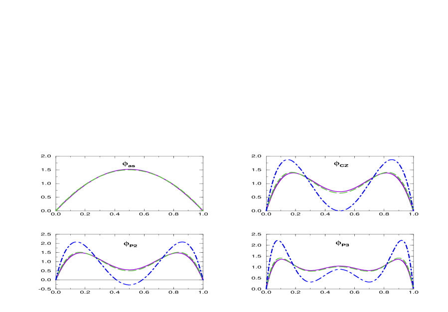
FIG. 6.: Evolution of the four candidate pion distribution amplitudes: $\phi_{as}(x,\mu_{F}^{2})$, $\phi_{CZ}(x,\mu_{F}^{2})$, $\phi_{P2}(x,\mu_{F}^{2})$, and $\phi_{P3}(x,\mu_{F}^{2})$, with the running coupling constant $\alpha_{S}(\mu_{F}^{2})$ and three active flavors. The dash-dotted curves correspond to the distribution amplitudes given by (III) and taken as nonperturbative input at the reference momentum scale $\mu_{0}^{2}=(0.5$ GeV$)^{2}$. The dashed curves correspond to the distribution amplitudes at the momentum scale $\mu_{F}^{2}=(2$ GeV$)^{2}$ with the LO evolutional corrections included according to (97) . The solid curves correspond to the distribution amplitudes at the momentum scale $\mu_{F}^{2}=(2$ GeV$)^{2}$ with the NLO evolutional corrections taken into account according to Eqs. (64) and (97–99).

IV Choosing the factorization and the renormalization scales

In this section we discuss various possibilities of choosing the renormalization scale $\mu_{R}$ and the factorization scale $\mu_{F}$ appropriate for the process under consideration.

Before starting the discussion, let us now, with the help of Eqs. (1), (3), and (64), write down the complete leading-twist NLO QCD expression for the pion electromagnetic form factor with the $\mu_{R}$ and $\mu_{F}$ dependence of all the terms explicitly indicated.

Generally, for the NLO form factor we can write

$$F_{\pi}(Q^{2},\mu_{R}^{2},\mu_{F}^{2})=F_{\pi}^{(0)}(Q^{2},\mu_{R}^{2},\mu_{F}^{2})+F_{\pi}^{(1)}(Q^{2},\mu_{R}^{2},\mu_{F}^{2})\,.$$ (104)

The first term in (104) is the LO contribution and is given by

$$F_{\pi}^{(0)}(Q^{2},\mu_{R}^{2},\mu_{F}^{2})=\int_{0}^{1}dx\,\int_{0}^{1}dy\quad\alpha_{S}(\mu_{R}^{2})\>\Phi^{LO*}(y,\mu_{F}^{2})\,T_{H}^{(0)}(x,y,Q^{2})\,\Phi^{LO}(x,\mu_{F}^{2})\,.$$ (105)

The second term in (104) is the NLO contribution and can be written as

$$F_{\pi}^{(1)}(Q^{2},\mu_{R}^{2},\mu_{F}^{2})=F_{\pi}^{(1a)}(Q^{2},\mu_{R}^{2},\mu_{F}^{2})+F_{\pi}^{(1b)}(Q^{2},\mu_{R}^{2},\mu_{F}^{2})\,,$$ (106)

where

$$F_{\pi}^{(1a)}(Q^{2},\mu_{R}^{2},\mu_{F}^{2})=\,\int_{0}^{1}dx\,\int_{0}^{1}dy\>\frac{\alpha_{S}^{2}(\mu_{R}^{2})}{\pi}\>$$ (108)

$$\qquad\qquad\times\,\Phi^{LO*}(y,\mu_{F}^{2})\,T_{H}^{(0)}(x,y,Q^{2})\,T_{H}^{(1)}(x,y,\mu_{R}^{2}/Q^{2},\mu_{F}^{2}/Q^{2})\,\Phi^{LO}(x,\mu_{F}^{2})\,,$$

is the contribution coming from the NLO correction to the hard-scattering amplitude, whereas

$$F_{\pi}^{(1b)}(Q^{2},\mu_{R}^{2},\mu_{F}^{2})=\int_{0}^{1}dx\,\int_{0}^{1}dy\quad\frac{\alpha_{S}(\mu_{R}^{2})\alpha_{S}(\mu_{F}^{2})}{\pi}$$ (110)

$$\quad\times\,\left[\Phi^{NLO*}(y,\mu_{F}^{2})\,T_{H}^{(0)}(x,y,Q^{2})\,\Phi^{LO}(x,\mu_{F}^{2})+\,\Phi^{LO*}(y,\mu_{F}^{2})\,T_{H}^{(0)}(x,y,Q^{2})\,\Phi^{NLO}(x,\mu_{F}^{2})\right]$$

is the contribution arising from the inclusion of the NLO evolution of the distribution amplitude. Now, if (6) is taken into account, the expression for the LO contribution of Eq. (105) can be written in the form

$$F_{\pi}^{(0)}(Q^{2},\mu_{R}^{2},\mu_{F}^{2})=\frac{8}{9}\,\pi\,\frac{f_{\pi}^{2}}{Q^{2}}\,\int_{0}^{1}dx\,\int_{0}^{1}dy\quad\alpha_{S}(\mu_{R}^{2})\>\frac{\phi^{LO}(x,\mu_{F}^{2})}{\overline{x}\,}\>\frac{\phi^{LO*}(y,\mu_{F}^{2})}{\overline{y}\,}\,.$$ (112)

Next, before going on to perform the remaining $x$ and $y$ integrations, we have to choose the renormalization scale $\mu_{R}$ and the factorization scale $\mu_{F}$. In doing this, however, there is considerable freedom involved.

If calculated to all orders in perturbation theory, the physical pion form factor $F_{\pi}(Q^{2})$, represented at the sufficiently high $Q^{2}$ by the factorization formula (1), would be independent of the renormalization and factorization scales, $\mu_{R}$ and $\mu_{F}$, and so they are arbitrary parameters. Truncation of the perturbative expansion of $F_{\pi}(Q^{2})$ at any finite order causes a residual dependence on these scales. Although the best choice for these scales remains an open question (the scale ambiguity problem), one would like to choose them in such a way that they are of order of some physical scale in the problem, and, at the same time, to reduce the size of higher-order corrections as much as possible. Choosing any specific value for these scales leads to a theoretical uncertainty of the perturbative result.

In our calculation we approximate $F_{\pi}(Q^{2})$ only by two terms of the perturbative series and hope that we can minimize higher-order corrections by a suitable choice of $\mu_{R}$ and $\mu_{F}$, so that the LO term $F_{\pi}^{(0)}(Q^{2},\mu_{R}^{2},\mu_{F}^{2})$ gives a good approximation to the complete sum $F_{\pi}(Q^{2})$.

It should be noted that in $F_{\pi}^{(0)}(Q^{2},\mu_{R}^{2},\mu_{F}^{2})$, given by (105), $\mu_{R}$ appears only through $\alpha_{S}(\mu_{R}^{2})$, whereas $\mu_{F}$ enters into the distribution amplitude $\phi(x,\mu_{F}^{2})$. In $F_{\pi}^{(1)}(Q^{2},\mu_{R}^{2},\mu_{F}^{2})$, given by (106–LABEL:eq:Fpi2b), a logarithmic dependence on the scales $\mu_{R}$ and $\mu_{F}$ appears also through $T_{H}^{(1)}(x,y,\mu_{R}^{2}/Q^{2},\mu_{F}^{2}/Q^{2})$. As seen from (II) and (47), this dependence is contained in the terms

$$f_{UV}(x,y,Q^{2}/\mu_{R}^{2}) = \frac{1}{4}\beta_{0}\left[\frac{5}{3}-\ln(\overline{x}\,\overline{y}\,)+\ln\frac{\mu_{R}^{2}}{Q^{2}}\right]\,,$$ (113)

$$f_{IR}(x,y,Q^{2}/\mu_{F}^{2}) = \frac{2}{3}[3+\ln(\overline{x}\,\overline{y}\,)]\left[\frac{1}{2}\ln(\overline{x}\,\overline{y}\,)-\ln\frac{\mu_{F}^{2}}{Q^{2}}\right]\,.$$ (114)

Being independent of each other, the scales $\mu_{R}$ and $\mu_{F}$ can be expressed in terms of $Q^{2}$ as

$$\mu_{R}^{2} = a(x,y)\,Q^{2}\,,$$ (115)

$$\mu_{F}^{2} = b(x,y)\,Q^{2}\,,$$ (116)

where $a(x,y)$ and $b(x,y)$ are some linear functions of the dimensionless variables $x$ and $y$ (quark longitudinal momentum fractions).

We next discuss various possibilities of choosing the scales $\mu_{R}$ and $\mu_{F}$ separately. The simplest and widely used choice for the scale $\mu_{R}$ is

$$\mu_{R}^{2}=Q^{2}\,,$$ (117)

the justification for the use of which is mainly pragmatic.

Physically, however, the more appropriate choice for $\mu_{R}^{2}$ would be that one corresponding to the characteristic virtualities of the particles in the parton subprocess, which is considerably lower than the overall momentum transfer $Q^{2}$ (i.e., virtuality of the probing photon).

It follows from Figs. 1 and 2 that the virtualities of the gluon line (line 4) and the internal quark line (line 2) of diagram A in Fig. 2 are given by $\overline{x}\,\overline{y}\,Q^{2}$ and $\overline{y}\,Q^{2}$, respectively. Now, if instead of using (117) we choose $\mu_{R}$ to be equal to the gluon virtuality, i.e.,

$$\mu_{R}^{2}=\overline{x}\,\overline{y}\,Q^{2}\,,$$ (118)

then the logarithmic terms in (113) vanish.

As it is well known, unlike in an Abelian theory (e.g., QED), where the effective coupling is entirely renormalized by the corrections of the vector particle propagator, in QCD the coupling is renormalized not only by the gluon propagator, but also by the quark-gluon vertex and quark-propagator corrections. It is thus possible to choose $\mu_{R}^{2}$ as the geometrical mean of the gluon and quark virtualities [6]:

$$\mu_{R}^{2}=\sqrt{(\overline{x}\,\overline{y}\,Q^{2})(\overline{y}\,Q^{2})}\,.$$ (119)

Alternatively, we can make a choice

$$\mu_{R}^{2}=e^{-5/3}\overline{x}\,\overline{y}\,Q^{2}\,,$$ (120)

as a result of which the function $f_{UV}$, given by (113), vanishes identically. In this case, $T_{H}^{(1)}(x,y,\mu_{R}^{2}/Q^{2},\mu_{F}^{2}/Q^{2})$ defined by (47) becomes $n_{f}$ independent. This is an example of choosing the renormalization scale according to the Brodsky-Lepage-Mackenzie (BLM) procedure [28]. In this procedure, the renormalization scale $\mu_{R}^{2}$ best suited to a particular process in a given order can be determined by computing vacuum-polarization insertions in the diagrams of that order. The essence of the BLM procedure is that all vacuum-polarization effects from the QCD $\beta$ function are resummed into the running coupling constant.

Let us just mention at this point that in addition to the BLM procedure, two more renormalization scale-setting procedures in PQCD have been proposed in the literature: the principle of fastest apparent convergence (FAC) [29], and the principle of minimal sensitivity (PMS) [30]. The application of those three quite distinct methods can give strikingly different results in practical calculations [31].

As for the factorization scale $\mu_{F}^{2}$, it basically determines how much of the collinear term given in (114), is absorbed into the distribution amplitude. A natural choice for this scale would be

$$\mu_{F}^{2}=Q^{2}\,,$$ (121)

which eliminates the logarithms of $Q^{2}/\mu_{F}^{2}$. More preferable to (121) is the choice

$$\mu_{F}^{2}=\sqrt{\overline{x}\,\overline{y}\,}Q^{2}\,,$$ (122)

which makes the function $f_{IR}$, given by (114), vanish.

A glance at Eqs. (104–LABEL:eq:Fpi2b), where the coupling constants $\alpha_{S}(\mu_{R}^{2})$ and $\alpha_{S}(\mu_{F}^{2})$ appear under the integral sign, reveals that any of the choices of $\mu_{R}$ given by (118–120), and the choice of $\mu_{F}$ given by (122), leads immediately to the problem if the usual one-loop formula (4) for the effective QCD running coupling constant is employed. Namely, then, regardless of how large $Q^{2}$ is, the integration of Eqs. (104–LABEL:eq:Fpi2b) allows $\alpha_{S}(\mu_{R}^{2})$ to be evaluated near zero momentum transfer. Two approaches are possible to circumvent this problem. First, one can choose $\mu_{R}^{2}$ and $\mu_{F}^{2}$ to be effective constants by taking $\mu_{R}^{2}=\left<\mu_{R}^{2}\right>$ and $\mu_{F}^{2}=\left<\mu_{F}^{2}\right>$, respectively. Second, one can introduce a cutoff in formula (4) with the aim of preventing the effective coupling from becoming infinite for vanishing gluon momenta.

If the first approach is taken, Eqs. (118–120) and (122) get replaced by the averages

$$\mu_{R}^{2} = \left<\overline{x}\,\overline{y}\,Q^{2}\right>\,,$$ (124)

$$\mu_{R}^{2} = \sqrt{\left<\overline{x}\,\overline{y}\,Q^{2}\right>\left<\overline{y}\,Q^{2}\right>}\,,$$ (125)

$$\mu_{R}^{2} = \left<e^{-5/3}\overline{x}\,\overline{y}\,Q^{2}\right>\,,$$ (126)

and

$$\mu_{F}^{2}=\sqrt{\left<\overline{x}\,\overline{y}\,\right>}Q^{2}\,,$$ (127)

respectively. Taking into account the fact that $\left<\overline{x}\,\overline{y}\,\right>=\left<\overline{x}\,\right>\left<\overline{y}\,\right>$ and $\left<\overline{x}\,\right>=\left<\overline{y}\,\right>$, it is possible to write Eqs. (IV) and (127) in the respective forms:

$$\mu_{R}^{2} = \left<\overline{x}\,\right>^{2}Q^{2}\,,$$ (129)

$$\mu_{R}^{2} = \left<\overline{x}\,\right>^{3/2}Q^{2}\,,$$ (130)

$$\mu_{R}^{2} = e^{-5/3}\left<\overline{x}\,\right>^{2}Q^{2}\,,$$ (131)

and

$$\mu_{F}^{2}=\left<\overline{x}\,\right>Q^{2}\,.$$ (132)

The key quantity in the above considerations is $\left<\overline{x}\,\right>$, the average value of the momentum fraction. It depends on the form of the distribution amplitude, and there is no unique way of defining it. A possible definition is

$$\left<\overline{x}\,\right>(\mu_{F}^{2})=\frac{\displaystyle\int_{0}^{1}dx\,\phi(x,\mu_{F}^{2})\,\overline{x}\,}{\displaystyle\int_{0}^{1}dx\,\phi(x,\mu_{F}^{2})}\,.$$ (133)

Owing to the fact that all distribution amplitudes under consideration are centered around the value $x=0.5$, it follows trivially from (133) that for all of them

$$\left<\overline{x}\,\right>(\mu_{F}^{2})=0.5\,.$$ (134)

An alternative way of defining $\left<\overline{x}\,\right>$, motivated by the form of the LO expression for the pion form factor (112), is

$$\left<\overline{x}\,\right>(\mu_{F}^{2})=\frac{\displaystyle\int_{0}^{1}dx\,\displaystyle\frac{\phi^{LO}(x,\mu_{F}^{2})}{\overline{x}\,}\,\overline{x}\,}{\displaystyle\int_{0}^{1}dx\,\displaystyle\frac{\phi^{LO}(x,\mu_{F}^{2})}{\overline{x}\,}}=\frac{1}{3[1+B_{2}^{LO}(\mu_{F}^{2})+B_{4}^{LO}(\mu_{F}^{2})+\ldots]}\,.$$ (135)

It should be noted, however, that this formula can be straightforwardly applied only if $\mu_{F}^{2}=Q^{2}$. On the other hand, if instead of $\mu_{F}^{2}=Q^{2}$ one chooses the factorization scale to be as given by (132), then Eqs. (132) and (135) form a nontrivial system of simultaneous equations. According to (135), one obtains $\left<\overline{x}\,\right>_{as}(Q^{2})=1/3$ for any $Q^{2}$, while $0.242\leq\left<\overline{x}\,\right>_{CZ}(Q^{2})\leq 0.262$ for $4\mbox{GeV}^{2}\leq Q^{2}\leq 100\mbox{GeV}^{2}$ (similar values are obtained for $\phi_{P2}$ and $\phi_{P3}$).

When using the $\phi_{as}(x,\mu_{F}^{2})$ distribution it appears reasonable to take $\left<\overline{x}\,\right>(\mu_{F}^{2})$= ${\left<\overline{x}\,\right>}_{as}$=1/2. This can be justified on the grounds that this distribution is concentrated around $x=0.5$, and is characterized by a very weak evolution. On the other hand, for the end-point concentrated distributions $\phi_{CZ}(x,\mu_{F}^{2})$, $\phi_{P2}(x,\mu_{F}^{2})$ and $\phi_{P3}(x,\mu_{F}^{2})$, which exibit sizable evolutional effects, it is more appropriate to take ${\left<\overline{x}\,\right>}(\mu_{F}^{2})$ as given by Eq. (135).

As stated above, the divergence of the effective QCD coupling $\alpha_{S}(\mu_{R}^{2})$, as given by (4), is the reason that it is not possible to use the choices of $\mu_{R}^{2}$ given by (118–120) and $\mu_{F}^{2}$ given by (122). Equation (4) does not represent the nonperturbative behavior of $\alpha_{S}(\mu_{R}^{2})$ for small $\mu_{R}^{2}$, and a number of proposals have been suggested for the form of the coupling constant in this regime [32]. The most exploited parameterization of the effective QCD coupling constant at low energies has the form

$$\alpha_{S}(\mu_{R}^{2})=\frac{4\pi}{\beta_{0}\ln\left(\displaystyle\frac{\mu_{R}^{2}+C^{2}}{\Lambda^{2}}\right)}\,,$$ (136)

where the constant $C$ encodes the nonperturbative dynamics and is usually interpreted as an “effective dynamical gluon mass” $m_{g}$. For $\mu_{R}^{2}\gg C^{2}$, the effective coupling in (136) coincides with the one-loop formula (4), whereas at low momentum transfer this formula “freezes” to some finite but not necessarily small value.

In view of the confinement phenomenon, the modification (136) is very natural: the lower bound on the particle momenta is set by the inverse of the confinement radius. This is equivalent to a strong suppression for the propagation of particles with small momenta. Thus, in a consistent calculation in which (136) is assumed a modified gluon propagator should be used:

$$\frac{1}{k^{2}}\rightarrow\frac{1}{k^{2}-m_{g}^{2}}\,.$$ (137)

However, if one attempts to calculate the LO prediction for the pion form factor making use of (136) and (137), and taking $m_{g}=300-500$ MeV, the result obtained is by a factor of $10$ lower than the experimental value, questioning the applicability of such an approach [15].

It has recently been shown that spontaneous chiral symmetry breaking imposes rather a severe restriction on the idea of freezing [33]. The authors of [33] argue that before any argument based on a particular form of the freezing coupling constant is put forward, one should check that the dynamical origin (mechanism) of the freezing is such that enough chiral symmetry breaking can be produced.

Considering the discussion above, calculations with the frozen coupling constant seem to need a more refined treatment and will not be considered in this paper.

V Complete NLO numerical predictions for the pion form factor

Having obtained all the necessary ingredients in the preceding sections, now we put them together and obtain complete leading-twist NLO QCD numerical predictions for the pion form factor. For a fixed distribution amplitude, we analyze the dependence of our results on the choice of the scales $\mu_{R}$ and $\mu_{F}$.

By inserting (80) and (82) into (105) and (LABEL:eq:Fpi2b), taking into account (6), taking the scales $\mu_{R}^{2}$ and $\mu_{F}^{2}$ to be effective constants (as explained in Sec. IV), and performing the $x$ and $y$ integration, we find that Eqs. (105) and (LABEL:eq:Fpi2b) take the form

$$Q^{2}F_{\pi}^{(0)}(Q^{2},\mu_{R}^{2},\mu_{F}^{2})=8\pi f_{\pi}^{2}\alpha_{S}(\mu_{R}^{2})\left(\sum_{n=0}^{\infty}{}^{\prime}B_{n}^{LO}(\mu_{F}^{2})\right)^{2}\,,$$ (138)

and

$$Q^{2}F_{\pi}^{(1b)}(Q^{2},\mu_{R}^{2},\mu_{F}^{2})=16f_{\pi}^{2}\alpha_{S}(\mu_{R}^{2})\alpha_{S}(\mu_{F}^{2})\left(\sum_{n=0}^{\infty}{}^{\prime}B_{n}^{LO}(\mu_{F}^{2})\right)\left(\sum_{k=2}^{\infty}{}^{\prime}B_{k}^{NLO}(\mu_{F}^{2})\right)\,.$$ (139)

For a distribution amplitude of the form given in (91 - 103), the above expression reduces to

$$Q^{2}F_{\pi}^{(0)}(Q^{2},\mu_{R}^{2},\mu_{F}^{2}) = 8\,\pi\,f_{\pi}^{2}\,\alpha_{S}(\mu_{R}^{2})\,\left[1+B_{2}^{LO}(\mu_{F}^{2})+B_{4}^{LO}(\mu_{F}^{2})\right]^{2}\,,$$ (140)

$$Q^{2}F_{\pi}^{(1b)}(Q^{2},\mu_{R}^{2},\mu_{F}^{2}) = 16\,f_{\pi}^{2}\,\alpha_{S}(\mu_{R}^{2})\,\alpha_{S}(\mu_{F}^{2})\,\left[1+B_{2}^{LO}(\mu_{F}^{2})+B_{4}^{LO}(\mu_{F}^{2})\right]\,$$ (142)

$$\times\left[B_{2}^{NLO}(\mu_{F}^{2})+B_{4}^{NLO}(\mu_{F}^{2})+\sum_{k=6}^{\infty}{}^{\prime}B_{k}^{NLO}(\mu_{F}^{2})\right]\,.$$

As for the part of the NLO contribution arising from the NLO correction to the hard-scattering amplitude, by inserting (47) and (97) into (108) and performing the $x$ and $y$ integration one obtains

$$Q^{2}F_{\pi}^{(1a)}(Q^{2},\mu_{R}^{2},\mu_{F}^{2}) = 8\,f_{\pi}^{2}\,\alpha_{S}^{2}(\mu_{R}^{2})\,\left\{\frac{9}{4}\left[1+B_{2}^{LO}(\mu_{F}^{2})+B_{4}^{LO}(\mu_{F}^{2})\right]^{2}\ln\frac{\mu_{R}^{2}}{Q^{2}}\right.$$ (146)

$$\left.+\frac{2}{3}\left[\frac{25}{6}B_{2}^{LO}(\mu_{F}^{2})+\frac{91}{15}B_{4}^{LO}(\mu_{F}^{2})\right]\left[1+B_{2}^{LO}(\mu_{F}^{2})+B_{4}^{LO}(\mu_{F}^{2})\right]\ln\frac{\mu_{F}^{2}}{Q^{2}}\right.$$

$$\left.+6.58+24.99\,B_{2}^{LO}(\mu_{F}^{2})+21.43\,(B_{2}^{LO}(\mu_{F}^{2}))^{2}\right.$$

$$\left.+32.81\,B_{4}^{LO}(\mu_{F}^{2})+32.55\,(B_{4}^{LO}(\mu_{F}^{2}))^{2}+53.37\,B_{2}^{LO}(\mu_{F}^{2})\,B_{4}^{LO}(\mu_{F}^{2})\right\}\,.$$

Then the NLO contribution to the “almost scaling” combination $Q^{2}F_{\pi}(Q^{2})$ is given by

$$Q^{2}F_{\pi}^{(1)}(Q^{2},\mu_{R}^{2},\mu_{F}^{2})=Q^{2}F_{\pi}^{(1a)}(Q^{2},\mu_{R}^{2},\mu_{F}^{2})+Q^{2}F_{\pi}^{(1b)}(Q^{2},\mu_{R}^{2},\mu_{F}^{2})\,,$$ (147)

while the total NLO prediction reads

$$Q^{2}F_{\pi}(Q^{2},\mu_{R}^{2},\mu_{F}^{2})=Q^{2}F_{\pi}^{(0)}(Q^{2},\mu_{R}^{2},\mu_{F}^{2})+Q^{2}F_{\pi}^{(1)}(Q^{2},\mu_{R}^{2},\mu_{F}^{2})\,.$$ (148)

For the purpose of this calculation we adopt the criteria according to which a perturbative prediction for $F_{\pi}(Q^{2})$ is considered reliable provided the following two requirements are met: first, corrections to the LO prediction are reasonably small ($<30\%$); second, the expansion parameter (effective QCD coupling constant) is acceptably small ($\alpha_{S}(\mu_{R}^{2})<0.3$ or $0.5$). Of course, one more requirement should be added to the above ones: consistency with experimental data. This requirement, however, is not of much use here since reliable experimental data for the pion form factor exist for $Q^{2}\leq 4$ GeV², i.e., well outside the region in which the perturbative treatment based on Eq. (1) is justified.

Currently available experimental data for the spacelike pion electromagnetic form factor $F_{\pi}(Q^{2})$ are shown in Fig. 7. The data are taken from Bebek et al. [35] and Amendolia et al. [36]. As stated in [35], the measurements corresponding to $Q^{2}=6.30$GeV² and $Q^{2}=9.77$GeV² are somewhat questionable. Thus, effectively, the data for $F_{\pi}(Q^{2})$ exist only for $Q^{2}$ in the range $Q^{2}\leq 4$GeV². The results of Ref. [35] were obtained from the extrapolation of the $\gamma^{*}p\rightarrow\pi^{+}n$ electroproduction data to the pion pole. It should also be mentioned that the analysis of Ref. [35] is subject to criticism which questions whether $F_{\pi}(Q^{2})$ was truly determined for $1\leq Q^{2}\leq 4$GeV² [37] (but see also Ref. [38]). The new data in this energy region are expected from the CEBAF experiment E-93-021.

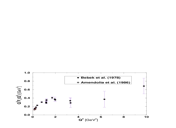
FIG. 7.: Presently available experimental data for the spacelike pion electromagnetic form factor.

A Predictions obtained with $\mu_{R}^{2}=\mu_{F}^{2}=Q^{2}$

The first NLO prediction for the pion form factor was obtained in Ref. [5]. Using the $\overline{MS}$ renormalization scheme and the choice $\mu_{R}^{2}=\mu_{F}^{2}=Q^{2}$ it was found that for the $\phi_{as}(x)$ distribution (with the evolution of the distribution amplitude neglected), the perturbative series took the form

$$Q^{2}F_{\pi}(Q^{2})=(0.43\mbox{ GeV}^{2})\,\alpha_{S}(Q^{2})\,[1+2.10\,\alpha_{S}(Q^{2})+\cdots]\,,$$ (149)

which is in agreement with our result given by (148), (140), and (146). The conclusion based on this result was that a reliable result for $F_{\pi}(Q^{2})$ was not obtained until $\alpha_{S}(Q^{2})\approx 0.1$, or with $\Lambda_{\overline{MS}}=0.5$ GeV, $Q^{2}=10000$ GeV². This prediction has been widely cited in the literature and initiated a lot of discussion regarding the applicability of PQCD to the calculation of exclusive processes at large momentum transfer. With the presently accepted value of 0.2 GeV for $\Lambda_{\overline{MS}}$, we find that the criteria from Ref. [5] are satisfied for $Q^{2}\sim 1600$ GeV², and that for $Q^{2}=700$ GeV², the corrections to the LO prediction are of order 30%. Thus, this result shows that for the choice of the renormalization and factorization scales $\mu_{R}^{2}=\mu_{F}^{2}=Q^{2}$, the region in which perturbative predictions can be considered reliable is still well beyond the region in which experimental data exist. The inclusion of the distribution amplitude evolution effects, although extremely important for the end-point concentrated amplitudes, does not change this conclusion.

Numerical results of our complete NLO QCD calculation, obtained using the four candidate distribution amplitudes, with $\mu_{R}^{2}=\mu_{F}^{2}=Q^{2}$, and for $Q^{2}\geq 4$ GeV², are displayed in Tables II, III, IV, and V. The entries in these tables include various contributions given by Eqs. (140–148), comprising the full NLO result. A comparison of our results with presently available experimental data is shown in Fig. 9. The ratio of the NLO to the LO contribution to $F_{\pi}(Q^{2})$, i.e., $F_{\pi}^{(1)}(Q^{2})/F_{\pi}^{(0)}(Q^{2})$, as a useful measure of the importance of the NLO corrections, is plotted as a function of $Q^{2}$ in Fig. 9. The shaded areas appearing in Figs. 9 and 9 denote the region of $Q^{2}$ where $\alpha_{S}(Q^{2})>0.3$. We take that outside of this region the effective coupling is acceptably small.

TABLE II.: Complete leading-twist NLO QCD results for the pion form factor, $Q^{2}F_{\pi}(Q^{2})$, obtained using the $\phi_{as}(x,\mu_{F}^{2})$ distribution amplitude and assuming $\mu_{R}^{2}=\mu_{F}^{2}=Q^{2}$.

$Q^{2}$	$\alpha_{S}(\mu_{R}^{2})$	$Q^{2}F_{\pi}^{(0)}(Q^{2})$	$Q^{2}F_{\pi}^{(1a)}(Q^{2})$	$Q^{2}F_{\pi}^{(1b)}(Q^{2})$	$Q^{2}F_{\pi}^{(1)}(Q^{2})$	$F_{\pi}^{(1)}(Q^{2})/F_{\pi}^{(0)}(Q^{2})$	$Q^{2}F_{\pi}(Q^{2})$
$[\mbox{GeV}^{2}]$		$[\mbox{GeV}^{2}]$	$[\mbox{GeV}^{2}]$	$[\mbox{GeV}^{2}]$	$[\mbox{GeV}^{2}]$	%	$[\mbox{GeV}^{2}]$
4	0.303	0.131	0.083	-0.001	0.082	62.8	0.213
6	0.279	0.120	0.070	-0.001	0.069	57.6	0.189
8	0.264	0.114	0.063	-0.001	0.062	54.4	0.176
10	0.253	0.109	0.058	-0.001	0.057	52.2	0.166
20	0.225	0.097	0.046	-0.001	0.045	46.2	0.142
30	0.211	0.091	0.040	-0.001	0.039	43.3	0.130
40	0.202	0.087	0.037	-0.001	0.036	41.4	0.123
50	0.196	0.085	0.035	-0.001	0.034	40.1	0.118
75	0.185	0.080	0.031	-0.001	0.030	37.9	0.110
100	0.178	0.077	0.029	-0.001	0.028	36.4	0.105

TABLE III.: Same as Table II but for the $\phi_{CZ}(x,\mu_{F}^{2})$ distribution amplitude.

$Q^{2}$	$\alpha_{S}(\mu_{R}^{2})$	$Q^{2}F_{\pi}^{(0)}(Q^{2})$	$Q^{2}F_{\pi}^{(1a)}(Q^{2})$	$Q^{2}F_{\pi}^{(1b)}(Q^{2})$	$Q^{2}F_{\pi}^{(1)}(Q^{2})$	$F_{\pi}^{(1)}(Q^{2})/F_{\pi}^{(0)}(Q^{2})$	$Q^{2}F_{\pi}(Q^{2})$
$[\mbox{GeV}^{2}]$		$[\mbox{GeV}^{2}]$	$[\mbox{GeV}^{2}]$	$[\mbox{GeV}^{2}]$	$[\mbox{GeV}^{2}]$	%	$[\mbox{GeV}^{2}]$
4	0.303	0.248	0.241	-0.015	0.225	90.8	0.474
6	0.279	0.222	0.195	-0.014	0.181	81.6	0.403
8	0.264	0.206	0.170	-0.013	0.157	76.1	0.363
10	0.253	0.195	0.153	-0.012	0.141	72.2	0.336
20	0.225	0.167	0.115	-0.011	0.104	62.2	0.271
30	0.211	0.154	0.098	-0.010	0.088	57.4	0.243
40	0.202	0.146	0.089	-0.009	0.079	54.3	0.225
50	0.196	0.140	0.082	-0.009	0.073	52.2	0.213
75	0.185	0.131	0.072	-0.008	0.064	48.7	0.194
100	0.178	0.125	0.065	-0.008	0.058	46.4	0.182

TABLE IV.: Same as Table II but for the $\phi_{P2}(x,\mu_{F}^{2})$ distribution amplitude.

$Q^{2}$	$\alpha_{S}(\mu_{R}^{2})$	$Q^{2}F_{\pi}^{(0)}(Q^{2})$	$Q^{2}F_{\pi}^{(1a)}(Q^{2})$	$Q^{2}F_{\pi}^{(1b)}(Q^{2})$	$Q^{2}F_{\pi}^{(1)}(Q^{2})$	$F_{\pi}^{(1)}(Q^{2})/F_{\pi}^{(0)}(Q^{2})$	$Q^{2}F_{\pi}(Q^{2})$
$[\mbox{GeV}^{2}]$		$[\mbox{GeV}^{2}]$	$[\mbox{GeV}^{2}]$	$[\mbox{GeV}^{2}]$	$[\mbox{GeV}^{2}]$	%	$[\mbox{GeV}^{2}]$
4	0.303	0.274	0.278	-0.019	0.259	94.6	0.532
6	0.279	0.244	0.224	-0.017	0.207	85.0	0.451
8	0.264	0.226	0.195	-0.016	0.179	79.1	0.404
10	0.253	0.213	0.175	-0.015	0.160	75.0	0.374
20	0.225	0.182	0.130	-0.013	0.117	64.5	0.300
30	0.211	0.167	0.111	-0.012	0.100	59.4	0.267
40	0.202	0.158	0.100	-0.011	0.089	56.2	0.247
50	0.196	0.152	0.093	-0.011	0.082	54.0	0.234
75	0.185	0.141	0.081	-0.010	0.071	50.2	0.212
100	0.178	0.134	0.074	-0.009	0.064	47.9	0.199

TABLE V.: Same as Table II but for the $\phi_{P3}(x,\mu_{F}^{2})$ distribution amplitude.

$Q^{2}$	$\alpha_{S}(\mu_{R}^{2})$	$Q^{2}F_{\pi}^{(0)}(Q^{2})$	$Q^{2}F_{\pi}^{(1a)}(Q^{2})$	$Q^{2}F_{\pi}^{(1b)}(Q^{2})$	$Q^{2}F_{\pi}^{(1)}(Q^{2})$	$F_{\pi}^{(1)}(Q^{2})/F_{\pi}^{(0)}(Q^{2})$	$Q^{2}F_{\pi}(Q^{2})$
$[\mbox{GeV}^{2}]$		$[\mbox{GeV}^{2}]$	$[\mbox{GeV}^{2}]$	$[\mbox{GeV}^{2}]$	$[\mbox{GeV}^{2}]$	%	$[\mbox{GeV}^{2}]$
4	0.303	0.335	0.402	-0.029	0.372	111.0	0.708
6	0.279	0.295	0.318	-0.026	0.292	100.0	0.587
8	0.264	0.272	0.273	-0.024	0.249	91.8	0.521
10	0.253	0.255	0.244	-0.023	0.222	86.7	0.477
20	0.225	0.215	0.178	-0.019	0.158	73.8	0.373
30	0.211	0.196	0.150	-0.017	0.133	67.7	0.328
40	0.202	0.184	0.134	-0.016	0.118	63.8	0.302
50	0.196	0.176	0.123	-0.015	0.108	61.1	0.284
75	0.185	0.163	0.106	-0.014	0.092	56.6	0.255
100	0.178	0.154	0.096	-0.013	0.083	53.7	0.237

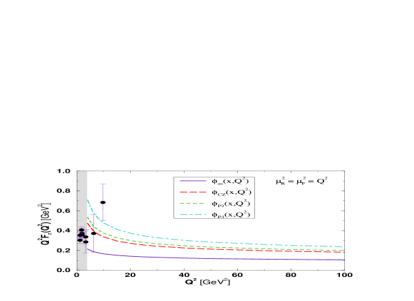
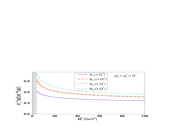
FIG. 8.: Comparison of the complete leading-twist NLO QCD predictions for the pion form factor, $Q^{2}F_{\pi}(Q^{2})$, obtained using the four candidate distribution amplitudes, with the presently available experimental data. The shaded area denotes the region of $Q^{2}$ in which $\alpha_{S}(Q^{2})\!>\!0.3$.

FIG. 9.: The ratio of the NLO to the LO contributions to the pion form factor, $F_{\pi}^{(1)}(Q^{2})/F_{\pi}^{(0)}(Q^{2})$, for the four candidate distribution amplitudes. The shaded area denotes the region of $Q^{2}$ in which $\alpha_{S}(Q^{2})\!>\!0.3$.

It is evident from Figs. 9 and 9 and Tables II–V that the leading-twist NLO results for the pion form factor obtained with $\mu_{R}^{2}=\mu_{F}^{2}=Q^{2}$ display the following general features. First, the results are quite sensitive to the assumed form of the pion distribution amplitude. Thus, the more end-point concentrated distribution amplitude is, the larger result for the pion form factor is obtained, and also the NLO corrections are larger (which has already been obvious looking at Eqs. (140-148)). Second, whereas the NLO correction arising from the corrections to the hard-scattering amplitude are positive, the corrections due to the inclusion of the evolutional corrections to the distribution amplitude are negative, with the former being generally an order of magnitude larger than the latter. Thus, in all the cases considered, the full NLO correction to the pion form factor is positive, i.e., its inclusion increases the LO prediction.

We now briefly comment on the results obtained with each of the four distribution amplitudes.

Table II, which corresponds to the $\phi_{as}(x,Q^{2})$ distribution amplitude, shows that the NLO correction $Q^{2}F_{\pi}^{(1)}(Q^{2})$ is rather large (36% at $Q^{2}=100$ GeV²). Most of the contribution to $Q^{2}F_{\pi}^{(1)}(Q^{2})$ is due to the NLO correction to the hard-scattering amplitude $Q^{2}F_{\pi}^{(1a)}(Q^{2})$, while the contribution $Q^{2}F_{\pi}^{(1b)}(Q^{2})$ arising from the NLO evolutional correction of the distribution amplitude is rather small, being of order 1%. The ratio $F_{\pi}^{(1)}(Q^{2})/F_{\pi}^{(0)}(Q^{2})\approx 30\%$ is reached at $Q^{2}\approx 500$ GeV².

The results derived from the $\phi_{CZ}(x,Q^{2})$ distribution are presented in Table III. The full NLO correction $Q^{2}F_{\pi}^{(1)}(Q^{2})$ is somewhat larger than for $\phi_{as}(x,Q^{2})$ (and at $Q^{2}=100$ GeV² it amounts to 46%). The ratio $F_{\pi}^{(1)}(Q^{2})/F_{\pi}^{(0)}(Q^{2})$ is greater than $30\%$ until $Q^{2}\approx 2400$ GeV². It is important to observe that the evolutional corrections, especially the LO ones, are rather significant in this case. Also, as it is seen from Table III, the NLO evolutional correction $Q^{2}F_{\pi}^{(1b)}(Q^{2})$ is of order $\approx 6\%$, i.e., nonnegligible. To show the importance of the correction arising from the inclusion of the distribution amplitude evolution, the results for $Q^{2}F_{\pi}(Q^{2})$ and the ratio $F_{\pi}^{(1)}(Q^{2})/F_{\pi}^{(0)}(Q^{2})$ obtained using the $\phi_{CZ}(x)$, $\phi_{CZ}^{LO}(x,Q^{2})$, and $\phi_{CZ}(x,Q^{2})$ distributions, are exhibited in Figs. 11 and 11, respectively.

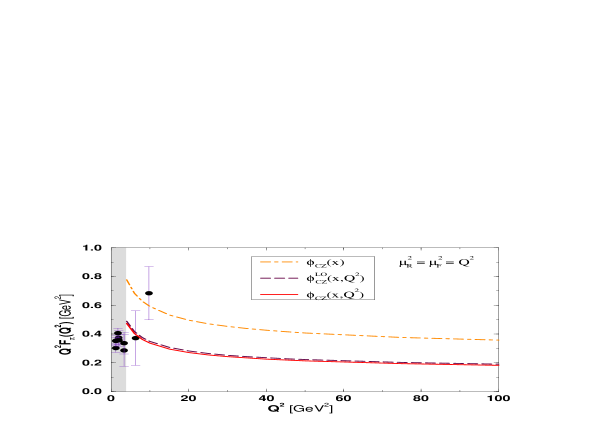
FIG. 10.: Leading-twist NLO QCD predictions for the pion form factor, $Q^{2}F_{\pi}(Q^{2})$, obtained with the $\phi_{CZ}(x)$, $\phi_{CZ}^{LO}(x,Q^{2})$, and $\phi_{CZ}(x,Q^{2})$ distributions. The shaded area denotes the region of $Q^{2}$ in which $\alpha_{S}(Q^{2})\!>\!0.3$.

FIG. 11.: The ratio of the NLO to the LO contributions to the pion form factor, $F_{\pi}^{(1)}(Q^{2})/F_{\pi}^{(0)}(Q^{2})$, obtained for the $\phi_{CZ}(x)$, $\phi_{CZ}^{LO}(x,Q^{2})$, and $\phi_{CZ}(x,Q^{2})$ distributions. The shaded area denotes the region of $Q^{2}$ in which $\alpha_{S}(Q^{2})\!>\!0.3$.

The results based on the $\phi_{P2}(x,Q^{2})$ and $\phi_{P3}(x,\mu_{F}^{2})$ distributions are listed in Table IV and V, respectively. As it can be easily seen by looking at Figs. 9 and 9 and by comparing the corresponding entries in Tables III and IV, the results obtained with the $\phi_{P2}(x,Q^{2})$ and $\phi_{CZ}(x,Q^{2})$ distributions are practically the same qualitatively, while differ quantitatively by a few percent. From Table V and Figs. 9 and 9, one can see that the behavior of the results obtained with the $\phi_{P3}(x,\mu_{F}^{2})$ distribution is qualitatively similar to the behavior of the results obtained with other two end-point concentrated distributions. For this reason, we leave the $\phi_{P2}(x,Q^{2})$ and $\phi_{P3}(x,\mu_{F}^{2})$ distributions out of our further consideration.

In view of what has been said above, we may conclude the following. If the pion is modeled by the $\phi_{as}(x,\mu_{F}^{2})$, $\phi_{CZ}(x,\mu_{F}^{2})$, $\phi_{P2}(x,\mu_{F}^{2})$, or $\phi_{P3}(x,\mu_{F}^{2})$ distribution amplitude, and if the renormalization and factorization scale are chosen to be $\mu_{R}^{2}=\mu_{F}^{2}=Q^{2}$, one finds that the NLO corrections to the lowest-order prediction for the pion form factor are large. The NLO predictions obtained cannot be made reliable, i.e., $F_{\pi}^{(1)}(Q^{2})/F_{\pi}^{(0)}(Q^{2})$ less than, say, 30 %, until the momentum transfer $Q\gg 10$ GeV is reached. Based on these findings and considering the region of $Q^{2}$ in which the data exist, it is clear that we are not in a position to rule out any of the four distributions considered. One can only note that the predictions for $Q^{2}F_{\pi}(Q^{2},\mu_{R}^{2},\mu_{F}^{2})$ obtained with the $\phi_{as}(x,\mu_{F}^{2})$ distribution are below the trend indicated by the existing experimental data, while the end-point concentrated distributions $\phi_{CZ}(x,\mu_{F}^{2})$, $\phi_{P2}(x,\mu_{F}^{2})$, and $\phi_{P3}(x,\mu_{F}^{2})$ give higher predictions. It is worth mentioning here that the theoretical predictions for the photon–to–pion transition form factor $F_{\pi\gamma}(Q^{2})$ are in very good agreement with the data, assuming the pion distribution amplitude is close to the asymptotic one, i.e., $\phi_{as}(x,\mu_{F}^{2})$ [39].

B Predictions obtained using $\mu_{R}^{2}=a\,Q^{2}$ and $\mu_{F}^{2}=b\,Q^{2}$

In this subsection we present a detailed analysis of the dependence of the complete leading$-$twist NLO predictions for the pion form factor obtained with the ${\phi}_{as}(x,\mu_{F}^{2})$ and ${\phi}_{CZ}(x,\mu_{F}^{2})$ distributions, on the renormalization and factorization scales, ${\mu}_{R}$ and ${\mu}_{F}$. In the following we shall restrict our attention to two most exploited pion distribution amplitudes ${\phi}_{as}(x,\mu_{F}^{2})$ and ${\phi}_{CZ}(x,\mu_{F}^{2})$.

In the preceding subsection, we have found that the NLO corrections calculated using these two distributions are large, especially for the latter. The reason for this lies in the fact that the renormalization scale choice $\mu_{R}^{2}=Q^{2}$ is not appropriate one. Namely, owing to the partitioning of the overall momentum transfer $Q^{2}$ among the particles in the parton subprocess, the essential virtualities of the particles are smaller than $Q^{2}$, so that the physical renormalization scale, better suited for analyzing the process under consideration, is inevitably lower than the external scale $Q^{2}$.

Compared with the scale $\mu_{R}$, the factorization scale $\mu_{F}$ turns out to be of secondary importance.

A characteristic feature of the asymptotic distribution ${\phi}_{as}(x,\mu_{F}^{2})$ is that in the LO it shows no evolution. A consequence of this, as it can be seen from Eqs. (140-148), is that the NLO predictions for the pion form factor based on this distribution are essentially independent of the factorization scale $\mu_{F}$. Namely, the only dependence on this scale is contained in the term arising from the NLO evolutional effects, which are tiny, as we have seen in Sec. III. On the other hand, the predictions calculated with the ${\phi}_{CZ}(x,\mu_{F}^{2})$ are ${\mu}_{F}$ dependent, but this dependence turns out to be very weak. Thus, for a given value of $\mu_{R}$, variation of the value of $\mu_{F}$ in the range $Q^{2}/4\leq\mu_{F}^{2}\leq Q^{2}$ leads to practically the same results. Therefore, when using the ${\phi}_{as}(x,\mu_{F}^{2})$ and ${\phi}_{CZ}(x,\mu_{F}^{2})$ distributions, one is allowed to set $\mu_{F}^{2}=Q^{2}$, for all practical purposes.

1 Examining the renormalization scale dependence of the NLO corrections

FIG. 12.: The numerical results for $Q^{2}F_{\pi}^{(0)}(Q^{2})$ obtained with the $\phi_{as}(x,\mu_{F}^{2})$ distribution amplitude and the choices of $\mu_{R}^{2}$ given by Eqs. (127), with $\mu_{F}^{2}=Q^{2}$ and $\left<\overline{x}\,\right>_{as}=1/2$. The solid curve (included for comparison) corresponds to the case $\mu_{R}^{2}=\mu_{F}^{2}=Q^{2}$ considered in the preceding subsection. The shaded area denotes the range of the LO prediction $Q^{2}F_{\pi}^{(0)}(Q^{2})$ for $\mu_{R}^{2}/Q^{2}\in\left[e^{-5/3}\left<\overline{x}\,\right>^{2},1\right]$.

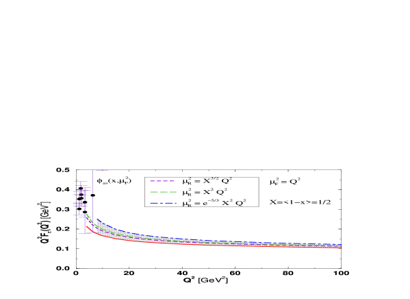
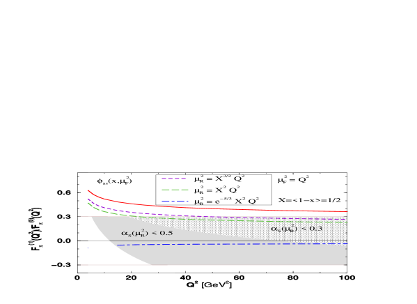
FIG. 13.: Leading-twist NLO QCD results for $Q^{2}F_{\pi}(Q^{2})$ obtained with the $\phi_{as}(x,\mu_{F}^{2})$ distribution amplitude and the choices of $\mu_{R}^{2}$ given by Eqs. (127), with $\mu_{F}^{2}=Q^{2}$ and $\left<\overline{x}\,\right>_{as}=1/2$. The solid curve (included for comparison) corresponds to the case $\mu_{R}^{2}=\mu_{F}^{2}=Q^{2}$ considered in the preceding subsection. The shaded area denotes the range of the total NLO prediction $Q^{2}F_{\pi}(Q^{2})$ where the upper limit corresponds to $\mu_{R}^{2}=\mu_{PMS}^{2}$ obtained from (154).

FIG. 14.: The ratio $F_{\pi}^{(1)}(Q^{2})/F_{\pi}^{(0)}(Q^{2})$ obtained with the $\phi_{as}(x,\mu_{F}^{2})$ distribution amplitude and the choices of $\mu_{R}^{2}$ given by Eqs. (127), with $\mu_{F}^{2}=Q^{2}$ and $\left<\overline{x}\,\right>_{as}=1/2$. The solid curve (included for comparison) is for the result corresponding to $\mu_{R}^{2}=\mu_{F}^{2}=Q^{2}$ obtained in the preceding subsection, and the shaded area denotes the region of the predictions which correspond to $\alpha_{S}(\mu_{R}^{2})\!<\!0.5$ ($\alpha_{S}(\mu_{R}^{2})\!<\!0.3$), while $|F_{\pi}^{(1)}(Q^{2})/F_{\pi}^{(0)}(Q^{2})|<0.3$.

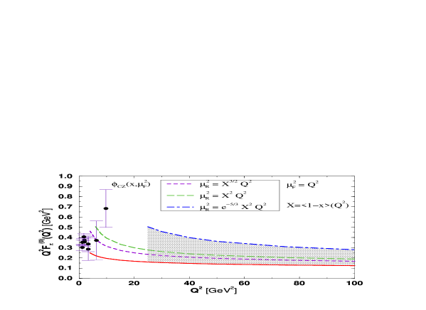
FIG. 15.: The numerical results for $Q^{2}F_{\pi}^{(0)}(Q^{2})$ obtained with the $\phi_{CZ}(x,\mu_{F}^{2})$ distribution amplitude and the choices of $\mu_{R}^{2}$ given by Eqs. (127), with $\mu_{F}^{2}=Q^{2}$ and $\left<\overline{x}\,\right>_{CZ}(Q^{2})$ calculated according to (135). The solid curve (included for comparison) corresponds to the case $\mu_{R}^{2}=\mu_{F}^{2}=Q^{2}$ considered in the preceding subsection. The shaded area denotes the range of the LO prediction $Q^{2}F_{\pi}^{(0)}(Q^{2})$ for $\mu_{R}^{2}/Q^{2}\in\left[e^{-5/3}\left<\overline{x}\,\right>^{2},1\right]$.

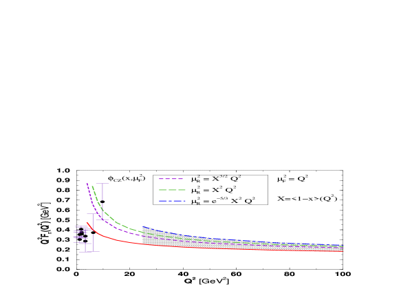
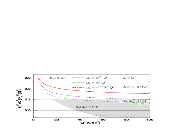
FIG. 16.: Leading-twist NLO QCD results for $Q^{2}F_{\pi}(Q^{2})$ obtained with the $\phi_{CZ}(x,\mu_{F}^{2})$ distribution amplitude and the choices of $\mu_{R}^{2}$ given by Eqs. (127), with $\mu_{F}^{2}=Q^{2}$ and $\left<\overline{x}\,\right>_{CZ}(Q^{2})$ calculated according to (135). The solid curve (included for comparison) corresponds to the case $\mu_{R}^{2}=\mu_{F}^{2}=Q^{2}$ considered in the preceding subsection. The shaded area denotes the range of the total NLO prediction $Q^{2}F_{\pi}(Q^{2})$ where the upper limit corresponds to $\mu_{R}^{2}=\mu_{PMS}^{2}$ obtained from (154).

FIG. 17.: The ratio $F_{\pi}^{(1)}(Q^{2})/F_{\pi}^{(0)}(Q^{2})$ obtained with the $\phi_{CZ}(x,\mu_{F}^{2})$ distribution amplitude and the choices of $\mu_{R}^{2}$ given by Eqs. (127), with $\mu_{F}^{2}=Q^{2}$ and $\left<\overline{x}\,\right>_{CZ}(Q^{2})$ calculated according to (135). The solid curve (included for comparison) is for the result corresponding to $\mu_{R}^{2}=\mu_{F}^{2}=Q^{2}$ obtained in the preceding subsection, and the shaded area denotes the region of the predictions which correspond to $\alpha_{S}(\mu_{R}^{2})\!<\!0.5$ ($\alpha_{S}(\mu_{R}^{2})\!<\!0.3$), while $|F_{\pi}^{(1)}(Q^{2})/F_{\pi}^{(0)}(Q^{2})|<0.3$.

The three specific physically motivated choices of ${\mu}_{R}$, given by (127), can be conveniently written as

$$\mu_{R}^{2}=a\,Q^{2},$$ (151)

where

$$a\in\{{\left<\overline{x}\,\right>}^{3/2},{\left<\overline{x}\,\right>}^{2},e^{-5/3}{\left<\overline{x}\,\right>}^{2}\}\,.$$ (152)

Our complete leading-twist NLO predictions for the pion form factor calculated with the ${\phi}_{as}(x,\mu_{F}^{2})$ distribution and with the three specific values of the renormalization scale ${\mu}_{R}$ are summarized in Figs. 14 and 14, showing the results for $Q^{2}F_{\pi}(Q^{2})$ and the ratio $F_{\pi}^{(1)}(Q^{2})/F_{\pi}^{(0)}(Q^{2})$, respectively. For the purpose of the discussion of the effects of the inclusion of the NLO corrections on the LO predictions, we have also included Fig. 12 showing the LO predictions for the three different values of ${\mu}_{R}$ given in Eq. (17). The corresponding results but obtained assuming the ${\phi}_{CZ}(x,\mu_{F}^{2})$ distribution are displayed in Figs. 15, 17, and 17.

The solid curves in Figs. 12 - 17 correspond to the results with $\mu_{R}^{2}=\mu_{F}^{2}=Q^{2}$ obtained in the preceding subsection, are included for comparison. The other curves refer to the choices of $\mu_{R}^{2}$ given by (17).

Some general comments concerning the results presented above are in order. First of all, it is interesting to note that the predictions based on the ${\phi}_{as}(x,\mu_{F}^{2})$ and ${\phi}_{CZ}(x,\mu_{F}^{2})$ distributions amplitudes almost share the qualitative features, although these two distributions are quite different in shape. Next, by looking at Figs. 14 and 17, one notices that the full NLO result for $Q^{2}F_{\pi}(Q^{2})$, shows a very weak dependence on the value of $\mu_{R}^{2}$, and that it increases with decreasing $\mu_{R}^{2}$. As far as the ratio $F_{\pi}^{(1)}(Q^{2})/F_{\pi}^{(0)}(Q^{2})$ is concerned, as evident from Figs. 14 and 17, the situation is quite different. It is rather sensitive to the variation of $\mu_{R}^{2}$, and decreases as $\mu_{R}^{2}$ decreases. The choice $\mu_{R}^{2}=Q^{2}$, represented by solid curves, when compared with the other possibilities considered, leads to the lowest value for $Q^{2}F_{\pi}(Q^{2})$, and to the highest value for the ratio $F_{\pi}^{(1)}(Q^{2})/F_{\pi}^{(0)}(Q^{2})$. In contrast to that, the choice of the BLM scale, represented by the dashed-dotted curve, leads to somewhat higher values of $Q^{2}F_{\pi}(Q^{2})$, but to considerably lower values of the ratio $F_{\pi}^{(1)}(Q^{2})/F_{\pi}^{(0)}(Q^{2})$.

Adopting the previously stated criteria, we now comment on the reliability of the NLO predictions for $Q^{2}F_{\pi}(Q^{2})$ displayed in Figs. 14 and 17. Imposing the requirements $\left|F_{\pi}^{(1)}(Q^{2})/F_{\pi}^{(0)}(Q^{2})\right|<0.3$, and ${\alpha}_{S}(\mu_{R}^{2})<0.3$, we find from Fig. 14 that for the ${\phi}_{as}(x,{\mu}_{F}^{2})$ distribution the results corresponding to $a={\left<\overline{x}\,\right>}^{3/2}$, ${\left<\overline{x}\,\right>}^{2}$, and $e^{-5/3}{\left<\overline{x}\,\right>}^{2}$, become reliable for the momentum transfer $Q^{2}>50$, $25$, and $90$ GeV², respectively. It might be that the requirement ${\alpha}_{S}(\mu_{R}^{2})<0.3$ is too stringent. Thus, by relaxing it and taking ${\alpha}_{S}(\mu_{R}^{2})<0.5$ instead, we find that the results corresponding to $a={\left<\overline{x}\,\right>}^{3/2}$, ${\left<\overline{x}\,\right>}^{2}$, and $e^{-5/3}{\left<\overline{x}\,\right>}^{2}$, become reliable for the momentum transfer $Q^{2}>50$, $25$, and $15$ GeV², respectively.

Applying the same criteria to the case of the ${\phi}_{CZ}(x,\mu_{R}^{2})$ distribution, we find from Fig. 17 that the results for $Q^{2}F_{\pi}(Q^{2})$, shown in Fig. 17, obtained with $a={\left<\overline{x}\,\right>}^{3/2}$, ${\left<\overline{x}\,\right>}^{2}$, and $e^{-5/3}{\left<\overline{x}\,\right>}^{2}$, become reliable for the momentum transfer $Q^{2}>95$, $60$, and $300$ GeV², respectively, if we demand that ${\alpha}_{S}(\mu_{R}^{2})<0.3$, and for $Q^{2}>95$, $35$, and $50$ GeV², respectively, if ${\alpha}_{S}(\mu_{R}^{2})<0.5$ is regarded as a stringent enough requirement.

Summarizing the above, one can say that contrary to the rather high value of $Q^{2}\approx 500$ GeV² required to obtain a reliable prediction assuming the ${\phi}_{as}(x,\mu_{R}^{2})$ distribution with $\mu_{R}^{2}=Q^{2}$, one finds that by choosing the renormalization scale determined by the dynamics of the pion rescattering process, the size of the NLO corrections is significantly reduced and reliable predictions are obtained at considerably lower values of $Q^{2}$, namely, for $Q^{2}<100$ GeV². The same conclusion also applies to the results obtained with the ${\phi}_{CZ}(x,\mu_{R}^{2})$ distribution, for which choosing the renormalization scale related to the virtuality of the particles in the parton subprocess lowers the bound of the reliability of the results from $Q^{2}\approx 2400$ GeV² to $Q^{2}<100$ GeV².

2 Theoretical uncertainty of the NLO predictions related to the renormalization scale ambiguity

Unfortunately, at present we do not have at our disposal any absolutely reliable method of determining the “optimal” (or “correct”) value of the renormalization scale for any particular order of PQCD. Our ignorance concerning the “optimal” value for ${\mu}_{R}$ implies that any particular choice of this scale leads to an intrinsic theoretical uncertainty (error) of the perturbative results. Therefore, the NLO results displayed in Figs. 14 and 17, being obtained with the four singled-out values of the renormalization scale ${\mu}_{R}$, contain theoretical uncertainty. In what follows we try to estimate this uncertainty. In order to do that, we have to make some assumptions, regarding the range of the renormalization scale ambiguity.

As already mentioned in addition to the BLM method, two more renormalization scale-settings have been proposed: the FAC and PMS methods. All three of them are somewhat ad hoc and have no strong justification. Nevertheless, the principles underlying these methods are plausible, so that they give us at least a range of scale ${\mu}_{R}$ which should be considered.

Let $\mu_{FAC}$, $\mu_{PMS}$, and $\mu_{BLM}$ designate the scales determined by the BLM, PMS, and FAC scale setting methods, respectively.

According to the FAC procedure, the scale ${\mu}_{R}$ is determined by the requirement that the NLO coefficient in the perturbative expansion of $F_{\pi}(Q^{2})$ vanishes, which, in our case, effectively reduces to solving the equation

$$F_{\pi}^{(1)}(Q^{2},\mu_{R}^{2}=\mu_{FAC}^{2})=0.$$ (153)

On the other hand, in the PMS procedure, one chooses the renormalization scale ${\mu}_{R}$ at the stationary point of the truncated perturbative series for $F_{\pi}(Q^{2})$. Operationally, this amounts to

$$\frac{dF_{\pi}(Q^{2},\mu_{R}^{2})}{d\mu_{R}^{2}}\left|{}_{\displaystyle\mu_{R}^{2}=\displaystyle\mu_{PMS}^{2}}\right.=0.$$ (154)

The BLM-determined scale is given by

$$\mu_{BLM}^{2}=e^{-5/3}\left<\overline{x}\,\right>^{2}Q^{2}\,.$$ (155)

The explicit expressions for $F_{\pi}(Q^{2})$ and $F_{\pi}^{(1)}(Q^{2})$ are given by (140-148) with $\mu_{F}^{2}=Q^{2}$. By solving Eqs. (153) and (154), and taking (155) into account we find that for the ${\phi}_{as}(x,{\mu}_{F}^{2})$ distribution:

$$\mu_{BLM}^{2}=Q^{2}/21\,,$$ (157)

$$\mu_{PMS}^{2}\approx Q^{2}/18\,,$$ (158)

$$\mu_{FAC}^{2}\approx Q^{2}/18\,,$$ (159)

while, for the ${\phi}_{CZ}(x,{\mu}_{F}^{2})$ distribution:

$$Q^{2}/79<\mu_{BLM}^{2}<Q^{2}/77\,,$$ (161)

$$Q^{2}/59<\mu_{PMS}^{2}<Q^{2}/54\,,$$ (162)

$$Q^{2}/53<\mu_{FAC}^{2}<Q^{2}/48\,,$$ (163)

for $50$ GeV${}^{2}<Q^{2}<100$ GeV². Therefore, we find that for both distributions

$$\mu_{BLM}^{2}<\mu_{PMS}^{2}<\mu_{FAC}^{2}\,.$$ (164)

The FAC, PMS, and BLM scales, as evident from (V B 2) and (V B 2), are very close to each other, and the curves corresponding to the NLO prediction for $Q^{2}F_{\pi}(Q^{2})$ obtained with the FAC and PMS scales practically coincide with the dashed-dotted curves in Figs. 14 and 17 corresponding to the BLM scale.

If the renormalization scale is interpreted as a “typical” scale of virtual momenta in the corresponding Feynman diagrams, then, despite the fact that we do not know what the “best” value of this scale is, it is (based on physical grounds and on the above considerations) reasonable to assume that it belongs to the interval ranging from ${\mu}_{BLM}^{2}$ to $Q^{2}$. Namely, ${\mu}_{BLM}^{2}$, being the lowest of the above considered scales and of the order of $Q^{2}/21$ and $Q^{2}/80$ for the ${\phi}_{as}(x,{\mu}_{F}^{2})$ and ${\phi}_{CZ}(x,{\mu}_{F}^{2})$ distributions, respectively, is a low enough to serve as the lower limit of the renormalization scale ambiguity interval. On the other hand, $Q^{2}$ is (too) high a scale and as such can safely be used for the upper limit of the same interval.

In the following, then, instead of using any singled-out value, we vary the renormalization scale in the form

$$\mu_{R}^{2}=a\,Q^{2}\,,$$ (166)

where $a$ is a continuous parameter

$$a\in[e^{-5/3}\left<\overline{x}\,\right>^{2},1]\,.$$ (167)

Doing this will enable us to draw some qualitative conclusions concerning, first, the theoretical uncertainty related to the renormalization scale ambiguity, and, second, the effects that the inclusion of the NLO corrections has on the LO predictions.

The LO result for the pion form factor is a monotonous function of the renormalization scale $\mu_{R}$. Namely, all of the $\mu_{R}$ dependence of the LO prediction $Q^{2}F_{\pi}^{(0)}(Q^{2})$, as it is seen from (140), is contained in the strong coupling constant $\alpha_{S}(\mu_{R}^{2})$. Thus, in accordance with (4), as $\mu_{R}$ decreases the LO result increases, and it increases without bound. In contrast to the LO, the NLO contribution $Q^{2}F_{\pi}^{(1)}(Q^{2})$, as evident from the explicit expression given in (146), decreases (becomes more negative) with decreasing $\mu_{R}$. Upon adding up the LO and NLO contributions, we find that the full NLO result, as a function of $\mu_{R}$ stabilizes and reaches a maximum value for $\mu_{R}^{2}=\mu_{PMS}^{2}$. The values of the scale $\mu_{PMS}$ are, for the $\phi_{as}(x,Q^{2})$ and $\phi_{CZ}(x,Q^{2})$ distributions given by (158) and (162), respectively.

If the renormalization scale continuously changes in the interval defined by (V B 2), we find that the curves representing the LO and NLO results for $Q^{2}F_{\pi}(Q^{2})$ fill out the shaded regions in Figs. 12 and 14, for the $\phi_{as}(x,Q^{2})$, and in Figs. 15 and 17 for the $\phi_{CZ}(x,Q^{2})$ distribution.

Next we turn to discuss the intrinsic theoretical uncertainty of the NLO prediction related to the renormalization scale ambiguity. Regarding this uncertainty, there is in fact no consensus on how to estimate it, or how to identify what the central value of $Q^{2}F_{\pi}(Q^{2})$ should be.

Nevertheless, the simplest but still a good measure of this uncertainty is the quantity

$${\Delta}F_{\pi}(Q^{2},{\mu}_{min}^{2},{\mu}_{max}^{2})=F_{\pi}(Q^{2},{\mu}_{min}^{2})-F_{\pi}(Q^{2},{\mu}_{max}^{2})\,,$$ (168)

i.e., the difference of the results for $F_{\pi}(Q^{2})$ corresponding to the lower and the upper limit of the renormalization scale ambiguity interval (V B 2). This quantity, therefore, for a given value of $Q^{2}$, represents the “width” of the shaded regions in Figs. 12, 14, 15, and 17. In this sense, the shaded regions in these figures limited by the curves corresponding to $\mu_{R}^{2}=Q^{2}$ and $\mu_{R}^{2}=\mu_{BLM}^{2}$ essentially determine the theoretical accuracy allowed by the LO and NLO calculation.

A glance at Figs. 12 and 14, displaying the LO and NLO predictions for $Q^{2}F_{\pi}(Q^{2})$ calculated with the $\phi_{as}(x,Q^{2})$ distribution, reveals that, compared to the LO, the NLO results exibit a much smaller renormalization scale dependence. The same holds true for the predictions depicted in Figs. 15 and 17, based on the $\phi_{CZ}(x,Q^{2})$ distribution.

To be more quantitative, we thus find that, if, for the $\phi_{as}(x,Q^{2})$ distribution, at $Q^{2}=50$ GeV² ($100$ GeV²), instead of ${\mu}_{R}^{2}=Q^{2}$ one takes ${\mu}_{R}^{2}=\mu_{BLM}^{2}=Q^{2}/21$, the LO result (Fig. 12) increases by $75\%$ ($64\%$), whereas the NLO result (Fig. 14) increases by $20\%$ ($16\%$). Analogously, for the same values of $Q^{2}$, but for the $\phi_{CZ}(x,Q^{2})$ distribution we find that taking ${\mu}_{R}^{2}=\mu_{BLM}^{2}\approx Q^{2}/79$ instead $\mu_{R}^{2}=Q^{2}$ the LO result increases by $158\%$ ($125\%$), while the NLO result increases by $47\%$ ($34\%$).

Therefore, the NLO corrections improve the situation because the terms in the NLO hard-scattering amplitude arise that cancel part of the scale dependence of the LO result.

It should be pointed out that our estimate of the renormalization scale ambiguity interval given in (V B 2) is very conservative, overestimating the theoretical uncertainty of the calculated NLO predictions. Namely, one could, almost at no risk replace $Q^{2}$ by $\left<\overline{x}\,\right>^{3/2}Q^{2}$ as the upper limit of the interval. If this is done, the dotted rather than solid curves would then provide the lower bound of the shaded regions in Figs. 14 and 17. Then, for $Q^{2}\geq 50$ GeV² theoretical uncertainty of the NLO result for $Q^{2}F_{\pi}(Q^{2})$ turns out to be less than $5\%$ for the $\phi_{as}(x,Q^{2})$ and $8\%$ for the $\phi_{CZ}(x,Q^{2})$ distribution.

Before closing this subsection, a remark is appropriate. If the shaded areas in Figs. 14 and 17 are displayed in the same figure they would not overlap. This implies that an unambiguous discrimination between the $\phi_{as}(x,Q^{2})$ and $\phi_{CZ}(x,Q^{2})$ distributions is possible, as soon as the data extending to higher values of $Q^{2}$ are obtained.

Based on the above considerations, we may conclude that the inclusion of the NLO corrections stabilizes the LO prediction for the pion form factor by considerably reducing the intrinsic theoretical uncertainty related to the renormalization scale ambiguity. This uncertainty for both distributions turns out to be of the order of a few percent.

VI Summary and conclusions

In this paper we have presented the results of a complete leading$-$twist NLO QCD analysis of the spacelike electromagnetic form factor of the pion at large momentum transfer.

To clarify the discrepancies in the analytical expression for the hard$-$scattering amplitude present in previous calculations, we have carefully recalculated the one$-$loop Feynman diagrams shown in Fig. 3. Working in the $\overline{\rm MS}$ renormalization scheme and employing the dimensional regularization method to treat all divergences (UV, IR, and collinear), we have obtained results which are in agreement with those of Refs. [5] (up to the typographical errors listed in [9]) and [7].

As nonperturbative input at the reference momentum scale of 0.5 GeV, we have used the four available pion distribution amplitudes defined by Eq. (III) and plotted in Fig. 5: the asymptotic distribution ${\phi}_{as}(x,{{\mu}_{F}}^{2})$ and the three QCD sum$-$rule inspired distributions ${\phi}_{CZ}(x,{{\mu}_{F}}^{2})$, ${\phi}_{P2}(x,{{\mu}_{F}}^{2})$, and ${\phi}_{P3}(x,{{\mu}_{F}}^{2})$. The NLO evolution of these distributions has been determined using the formalism developed in Ref. [20].

By convoluting, according to Eq. (1), the hard-scattering amplitude with the pion distribution amplitude, both calculated in the NLO approximation, we have obtained the NLO numerical predictions for the pion form factor, for the four candidate distributions, and for several different choices of the renormalization and factorization scales, ${\mu}_{R}$ and ${\mu}_{F}$. All the predictions have been obtained assuming $n_{f}=3$ and ${\Lambda}_{\overline{MS}}$=0.2 GeV.

We have first used the most simple choice of the scales where ${{\mu}_{R}}^{2}={{\mu}_{F}}^{2}=Q^{2}$. The results are summarized in Figs. 9 and 9 and Tables II–V. Although the predictions for the pion form factor $Q^{2}F_{\pi}(Q^{2})$ obtained with the four candidate distributions differ considerably, the lack of reliable experimental data, especially in the higher $Q^{2}$ region, does not allow us to confirm or discard any of them. The size of the NLO corrections and the size of the running coupling constant at given $Q^{2}$ can be used as indicators of the reliability of the perturbative treatment. Our numerical results based on the asymptotic distribution amplitude ${\phi}_{as}(x,{{\mu}_{F}}^{2})$ differ from those of Ref. [5] (the difference is due to the different value of $\Lambda_{\overline{MS}}$). Thus, in contrast to Ref. [5], where it was concluded that “reliable perturbative predictions can not be made until momentum transfers Q of about 100 GeV are reached”, we have found that reliable predictions can already be made at momentum transfers of the order of 25 GeV. It has been shown that the inclusion of the (NLO) evolutional corrections only slightly influences the NLO prediction obtained assuming the $\phi_{as}(x,\mu_{F}^{2})$ distribution. On the other hand, for the case of the end-point concentrated distributions, the evolutional corrections, both the LO and the NLO, are important. For the $\mu_{R}^{2}=\mu_{F}^{2}=Q^{2}$ choice of scales, the NLO corrections based on the $\phi_{as}(x,\mu_{F}^{2})$, $\phi_{CZ}(x,\mu_{F}^{2})$ $\phi_{P2}(x,\mu_{F}^{2})$, and $\phi_{P3}(x,\mu_{F}^{2})$ distributions, are large, which implies that one must demand that the momentum transfer $Q$ be considerably larger than $10$ GeV before the corresponding results become reliable.

In order to reduce the size of the NLO corrections and to examine the extent to which the NLO predictions for the pion form factor depend on the scales ${\mu}_{R}$ and ${\mu}_{F}$, in addition to the simplest choice ${{\mu}_{R}}^{2}={{\mu}_{F}}^{2}=Q^{2}$ (which certainly is not best suited for the process of interest), we have also considered the choices of ${\mu}_{R}$ and ${\mu}_{F}$ given by Eqs. (127) and (132), respectively. The results appear to be insensitive to the choice of $\mu_{F}$ considered. Using alternative choices for $\mu_{R}$, and modeling the pion with the ${\phi}_{as}(x,Q^{2})$ and ${\phi}_{CZ}(x,Q^{2})$ distribution amplitudes, leads to the predictions shown in Figs. 14, 14, 17, and 17. The ${\phi}_{P2}(x,{{\mu}_{F}}^{2})$ and ${\phi}_{P3}(x,{{\mu}_{F}}^{2})$ distributions are not separately considered, since the corresponding results are very similar to those obtained with ${\phi}_{CZ}(x,{{\mu}_{F}}^{2})$.

For a given distribution amplitude, the values of the pion form factor $Q^{2}F_{\pi}(Q^{2})$ are rather insensitive to various choices of the scales ${\mu}_{R}$. This is evident from Figs. 14 and 17, and is a reflection of the stabilizing effect that the inclusion of the NLO corrections has on the LO predictions. On the other hand, the ratio of the NLO corrections to the LO prediction, $F_{\pi}^{(1)}(Q^{2})/F_{\pi}^{(0)}(Q^{2})$ is very sensitive to the values of ${\mu}_{R}$, as can be seen from Figs. 14 and 17. Requiring this ratio to be less than $0.3$ and taking the less stringent condition on the value of the strong coupling $\alpha_{S}(\mu_{R}^{2})<0.5$, we find that the predictions can be considered reliable for the momentum transfer $Q<10$ GeV, provided the renormalization scale related to the average virtuality of the particles in the parton subprocess or given by the BLM scale, is used.

Given the fact that we do not know what the “optimal” value of the renormalization scale is, choosing any particular value for this scale introduces a theoretical uncertainty in the NLO predictions. Based on a reasonable guess of the renormalization scale ambiguity interval, we have estimated this uncertainty to be less than $10\%$.

The difference between the absolute predictions based on the $\phi_{as}(x,\mu_{F}^{2})$, $\phi_{CZ}(x,\mu_{F}^{2})$ ($\phi_{P2}(x,\mu_{F}^{2})$), and $\phi_{P3}(x,\mu_{F}^{2})$ distributions is large enough to allow an unambiguous experimental discrimination between them, as soon as the data extending to higher values of $Q$ become available.

In conclusion, the results of the complete leading-twist NLO QCD analysis, which has been carried out in this paper, show that reliable perturbative predictions for the pion electromagnetic form factor with all the four distribution amplitudes considered can already be made at a momentum transfer $Q<10$ GeV. The theoretical uncertainty related to the renormalization scale ambiguity, which constitutes a reasonable range of physical values, has been shown to be less than $10\%$. To check our predictions and to choose between the distribution amplitudes, it is necessary that experimental data at higher values of $Q^{2}$ are obtained.

- [1] S. J. Brodsky and G. P. Lepage, Phys. Lett. 87B, 359 (1979); Phys. Rev. Lett. 43, 545 (1979); Phys. Rev. Lett. 43, 1625 (1979) (E); G. P. Lepage and S. J. Brodsky, Phys. Rev. D 22, 2157 (1980).
- [2] A. V. Efremov and A. V. Radyushkin, Theor. Mat. Phys. 42, 97 (1980); Phys. Lett. 94B, 245 (1980).
- [3] A. Duncan and A. H. Mueller, Phys. Lett. 90B, 159 (1980); Phys. Rev. D 21, 1636 (1980).
- [4] S. J. Brodsky and G. P. Lepage, in Perturbative QCD, edited by A. H. Mueller (World Scientific Publishing Co., Singapore, 1989); V. L. Chernyak, in High Physics and Higher Twists, Proceedings of the Conference, Paris, France, 1988, edited by M. Benayoun, M. Fontannaz, and J. L. Narjoux, [Nucl. Phys. Proc. Suppl. 7B, 297 (1989)].
- [5] R. D. Field, R. Gupta, S. Otto, and L. Chang, Nucl. Phys. B186, 429 (1981).
- [6] F.-M. Dittes and A. V. Radyushkin, Yad. Fiz. 34, 529 (1981), [Sov. J. Nucl. Phys. 34, 293 (1981) ].
- [7] M. H. Sarmadi, Ph. D. thesis, University of Pittsburgh, 1982.
- [8] R. S. Khalmuradov and A. V. Radyushkin, Yad. Fiz. 42, 458 (1985), [Sov. J. Nucl. Phys. 42, 289 (1985)].
- [9] E. Braaten and S.-M. Tse, Phys. Rev. D 35, 2255 (1987).
- [10] E. P. Kadantseva, S. V. Mikhailov, and A. V. Radyushkin, Yad. Fiz. 44, 507 (1986), [Sov. J. Nucl. Phys. 44, 326 (1986) ].
- [11] F. D. Aguila and M. K. Chase, Nucl. Phys. B193, 517 (1981).
- [12] E. Braaten, Phys. Rev. D 28, 524 (1983).
- [13] B. Nižić, Phys. Rev. D 35, 80 (1987).
- [14] N. Isgur and C. H. Llewellyn Smith, Phys. Rev. Lett. 52, 1080 (1984); Phys. Lett. 217B, 535 (1989); Nucl. Phys. B 317, 526 (1989).
- [15] A. V. Radyushkin, Nucl. Phys. A 532, 141 (1991).
- [16] H.-N. Li and G. Sterman, Nucl. Phys. B 381, 129 (1992); D. Tung and H.-N. Li, Chin. J. Phys. 35, 651 (1997).
- [17] R. Jakob and P. Kroll, Phys. Lett. 315B, 463 (1993); ibid. 319B, 545 (E) (1993).
- [18] F.-M. Dittes and A. V. Radyushkin, Phys. Lett. 134B, 359 (1984); M. H. Sarmadi, ibid. 143B, 471 (1984); G. R. Katz, Phys. Rev. D 31, 652 (1985); S. V. Mikhailov and A. V. Radyushkin, Nucl. Phys. B254, 89 (1985).
- [19] S. V. Mikhailov and A. V. Radyushkin, Nucl. Phys. B273, 297 (1986).
- [20] D. Müller, Phys. Rev. D 49, 2525 (1994); Phys. Rev. D 51, 3855 (1995).
- [21] G. Curci, W. Furmanski, and R. Petronzio, Nucl. Phys. B175, 27 (1980).
- [22] S. J. Brodsky, P. Damgaard, Y. Frishman, and G. P. Lepage, Phys. Rev. D 33, 1881 (1986).
- [23] V. L. Chernyak and A. R. Zhitnitsky, Phys. Rep. 112, 173 (1984).
- [24] G. Martinelli and C. Sacharadja, Phys. Lett. 190B, 151 (1987); Phys. Lett. 217B, 319 (1989).
- [25] E. G. Floratos, D. A. Ross, and C. T. Sachrajda, Nucl. Phys. B129, 66 (1977); ibid. B 139, 545 (E) (1978).
- [26] A. Gonzales-Arroyo, C. Lopez, and F. J. Yndurain, Nucl. Phys. B153, 161 (1979).
- [27] G. R. Farrar, K. Huleihel, and H. Zhang, Nucl. Phys. B349, 655 (1991).
- [28] S. J. Brodsky, G. P. Lepage, and P. B. Mackenzie, Phys. Rev. D 28, 228 (1983).
- [29] G. Grunberg, Phys. Lett. 95B, 70 (1980); Phys. Lett. 110B, 501 (1982); Phys. Rev. D 29, 2315 (1984).
- [30] P. M. Stevenson, Phys. Lett. 100B, 61 (1981); Phys. Rev. D 23, 2916 (1981); Nucl. Phys. B203, 472 (1982); Nucl. Phys. B231, 65 (1984).
- [31] G. Kramer and B. Lampe, Z. Phys. A 339, 189 (1991).
- [32] G. Parisi and R. Petronzio, Phys. Lett. 94B, 51 (1980); A. C. Mattingly and P. M. Stevenson, Phys. Rev. D 49, 437 (1994); V. N. Gribov, Lund Report No. LU-TP 91-7, 1991 (unpublished); K. D. Born, E. Laermann, R. Sommer, P. M. Zerwas, and T. F. Walsh, Phys. Lett. 329B, 325 (1994); J. M. Cornwall, Phys. Rev. D 26, 1453 (1982); A. Donnachie and P. V. Landshoff, Nucl. Phys. B311, 509 (1989).
- [33] S. Peris and E. de Rafael, Nucl. Phys. B500, 325 (1997).
- [34] M. B. Gay Ducati, F. Halzen, and A. A. Natale, Phys. Rev. D 48, 2324 (1993).
- [35] J. Bebek et al., Phys. Rev. D 17, 1693 (1978).
- [36] S. R. Amendolia et al., Nucl. Phys. B277, 168 (1986).
- [37] C. E. Carlson and J. Milana, Phys. Rev. Lett. 65, 1717 (1990).
- [38] S. Dubnička and L. Martinovič, Phys. Rev. D 39, 2079 (1989); J. Phys. G 15, 1349 (1989).
- [39] A. V. Radyushkin, Acta Phys. Polon. B26, 2067 (1995); S. Ong, Phys. Rev. D 52, 3111 (1995); P. Kroll and M. Raulfs, Phys. Lett. 387B, 848 (1996).