section0.  subsection0.0.   
MPI-Ph/97-043 DESY 97-208
TUM-HEP-281/97 hep-ph/9802202

Determination of the CKM angle $\gamma$ and $|V_{ub}/V_{cb}|$ from inclusive direct CP asymmetries and branching ratios in charmless $B$ decays
Alexander Lenz,
Max-Planck-Institut für Physik — Werner-Heisenberg-Institut,
Föhringer Ring 6, D-80805 München, Germany,
Ulrich Nierste,
DESY - Theory group, Notkestrasse 85, D-22607 Hamburg, Germany,
and
Gaby Ostermaier
Physik-Department, TU München, D-85747 Garching, Germany

Abstract

We have calculated inclusive direct CP-asymmetries for charmless $B^{\pm}$–decays. After summing large logarithms to all orders the CP-asymmetries in $\Delta S=0$ and $\Delta S=1$ decays are found as

$$a_{CP}\left(\Delta S=0\right)\;=\;\left(2.0\raisebox{-2.15277pt}{\shortstack[l]{$\scriptstyle+1.2$\\ $\scriptstyle-1.0$}}\right)\%, \qquad a_{CP}\left(\Delta S=1\right)\;=\;\left(-1.0\pm 0.5\right)\%.$$

These results are much larger than previous estimates based on a work without summation of large logarithms. We further show that the dominant contribution to $a_{CP}\left(\Delta S=0\right)$ is proportional to $\sin\gamma\cdot|V_{cb}/V_{ub}|$. The constraints on the apex $(\overline{\rho},\overline{\eta})$ of the unitarity triangle obtained from these two CP-asymmetries define circles in the $(\overline{\rho},\overline{\eta})$-plane. We have likewise analyzed the information on the unitarity triangle obtainable from a measurement of the average non-leptonic branching ratios $\overline{Br}(\Delta S=0)$, $\overline{Br}(\Delta S=1)$ and their sum $\overline{Br}_{NL}(B\rightarrow\textit{no charm})$. These CP-conserving quantities define circles centered on the $\overline{\rho}$-axis of the $(\overline{\rho},\overline{\eta})$-plane. We expect a determination of $|V_{ub}/V_{cb}|$ from $\overline{Br}_{NL}(B\rightarrow\textit{no charm})$ to be promising. Our results contain some new QCD corrections enhancing $\overline{Br}(\Delta S=1)$, which now exceeds $\overline{Br}(\Delta S=0)$ by roughly a factor of two.

1 Introduction

CP-violation is a litmus test for the Standard Model, which parametrizes all CP-violating quantities by a single parameter, the complex phase in the Cabibbo-Kobayashi-Maskawa (CKM) matrix. The related amplitudes are further suppressed due to the smallness of CKM elements and loop graphs, so that new physics effects may become detectable. CP-violating observables are commonly expressed in terms of the angles $\alpha$, $\beta$ and $\gamma$ of the unitarity triangle. Yet we can determine its shape not only from its angles, but also from the length of its sides, which are obtained from measurements of CP-conserving quantities. This interplay is a special feature of the CKM mechanism. In order to overconstrain the unitarity triangle one must find sufficiently many theoretically clean observables. While, for example, $\beta$ can be extracted without hadronic uncertainties from the mixing-induced CP asymmetry in $B_{d}\rightarrow J/\psi K_{S}$, the angle $\gamma$ is notoriously hard to measure in experiments with $B_{d}$ and $B^{\pm}$ mesons.

Direct CP-violation in exclusive $B^{\pm}$-decays does not help to determine any of the angles because of the unknown strong phases in the decay amplitudes. On the contrary direct inclusive CP-asymmetries can be cleanly predicted, because quark-hadron duality allows the reliable calculation of strong interaction effects within perturbation theory. Such direct inclusive asymmetries have been analyzed in [1, 2, 3, 4, 5, 6] and mixing-induced inclusive CP-asymmetries studied in [7] are now investigated by the SLD collaboration [8]. Semi-inclusive direct CP-asymmetries have been studied in [9]. While inclusive final states are experimentally difficult to identify, inclusive branching ratios are huge compared to exclusive ones. As we will see in the following, inclusive CP-asymmetries in charmless decays have a promising size, so that it is worthwile to study them experimentally. Further they can be obtained from branching ratios only and therefore do not require an asymmetric $B$-factory.

In this paper we calculate direct inclusive CP-asymmetries in charmless $B^{\pm}$-decays extending our recent calculation of decay rates in [10]. In [10] the corresponding branching ratios have been calculated in renormalization group improved perturbation theory including the dominant contributions of the next-to-leading order. In the following section we set up our notations and summarize previous work on the subject. In sect. 3 we analyze $\Delta S=0$ decays. We discuss the relation of the CP-asymmetries to the angles of the unitarity triangle and their impact on the determination of the improved Wolfenstein parameters $\overline{\rho}$ and $\overline{\eta}$. Here we also investigate the constraint on $(\overline{\rho},\overline{\eta})$ imposed by a measurement of the average branching ratio of $B$ and $\overline{B}$ decays with $\Delta S=0$. In sect. 4 we repeat the procedure for $\Delta S=1$ decays. Readers mainly interested in phenomenology may draw their attention to sect. 5, where we will give numerical predictions for the newly calculated quantities. In sect. 5 we also predict the total charmless non-leptonic branching ratio of the $B$ meson and exemplify how the unitarity triangle is constructed from the branching ratios and CP-asymmetries. Finally we summarize our findings. An appendix contains details of our analytical results.

2 Preliminaries

We start our discussion with $B$ decays corresponding to the quark level transition $b\rightarrow q\overline{q}d$, $q=u,d,s,c$. They are triggered by the $|\Delta B|=1$, $|\Delta S|=0$ hamiltonian $H$:

$$H = \frac{G_{F}}{\sqrt{2}}\left\{\sum_{j=1}^{2}C_{j}\left(\xi_{c}^{*}Q_{j}^{c}+\xi_{u}^{*}Q_{j}^{u}\right)-\xi_{t}^{*}\sum_{j\in\mathcal{P}}C_{j}Q_{j}\right\}+h.c.\;,\qquad\qquad\xi_{q}\;=\;V_{qb}^{*}V_{qd}\;.$$ (1)

Here $Q_{1,2}^{c,u}$ are the familiar current-current operators, which originate from the tree-level $W$-exchange in $b\rightarrow c\overline{c}d$ and $b\rightarrow u\overline{u}d$. Further $\mathcal{P}=\{3,\ldots 6,8\}$, and $Q_{3-6}$ and $Q_{8}$ are the penguin operators. More details can be found in [10], where the numerical values for the Wilson coefficients $C_{i}$ are tabulated. For the following we only have to keep in mind that the coefficients $C_{3-6}$ and $C_{8}$ accompanying $\xi_{t}^{*}$ are much smaller in magnitude than $C_{1}$ and $C_{2}$.

Now we express the decay rate for $b\rightarrow q\overline{q}d$ as

$$\Gamma = \frac{G_{F}^{2}m_{b}^{5}}{64\pi^{3}}\cdot{\rm Re}\,\left[\left|\xi_{u}\right|^{2}\Gamma_{uu}+\left|\xi_{t}\right|^{2}\Gamma_{tt}+\left|\xi_{c}\right|^{2}\Gamma_{cc}+\xi_{u}\xi_{c}^{*}\Gamma_{uc}+\xi_{t}\xi_{u}^{*}\Gamma_{tu}+\xi_{t}\xi_{c}^{*}\Gamma_{tc}\right].$$ (2)

The coefficients $\Gamma_{ij}$ encode the various contributions of the different operators in (1). For example in $b\rightarrow u\overline{u}d$ the interference of the tree diagram of $Q_{2}^{u}$ in Fig. 2 with the penguin diagram of $Q_{2}^{c}$ with $q^{\prime}=c$ in Fig. 2 contributes to $\Gamma_{uc}$. The average branching ratio for the decay of $B^{\pm}$ into some inclusive final state $X$ reads

$$\overline{Br} = \frac{\Gamma\left(B^{+}\rightarrow X\right)+\Gamma\left(B^{-}\rightarrow\overline{X}\right)}{2\Gamma_{tot}}.$$ (3)

Similarly we define the CP-asymmetries as

$$A_{CP} = \frac{1}{2}\left[Br\left(B^{+}\rightarrow X\right)-Br\left(B^{-}\rightarrow\overline{X}\right)\right],\qquad\quad a_{CP}\;=\;\frac{A_{CP}}{\overline{Br}}.$$ (4)

Of course the average branching ratio in (3) may also be considered for $B_{d}$ and $\overline{B}_{d}$ instead of $B^{+}$ and $B^{-}$. We do not consider small spectator effects in this work, so that all given formulae for $\overline{Br}$ likewise apply to the neutral $B$ mesons. We will classify the inclusive final state $X$ by its strangeness quantum number $S$. Hence if also $B_{s}$ mesons are included in the consideration of $\overline{Br}$, the strangeness of $X$ must be corrected for the non-zero strangeness of the spectator quark.

Our strategy is to express $\overline{Br}$ and the CP-asymmetries in (4) in terms of the $\Gamma_{ij}$’s. The constraints for the CKM matrix obtained from measurements of $\overline{Br}$ and $a_{CP}$ are most conveniently expressed in terms of the improved Wolfenstein parameters $(\overline{\rho},\overline{\eta})$ [11]. The calculation of $(\overline{\rho},\overline{\eta})$ from $\overline{Br}$ and $a_{CP}$ involves certain combinations of the $\Gamma_{ij}$’s, for which we will derive compact approximate formulae. The exact expressions for the $\Gamma_{ij}$’s can be found in the appendix.

 

Figure 1: Tree diagram of $Q^{u}_{1,2}$.

Figure 2: Penguin diagram involving $Q_{2}^{q^{\prime}}$. It contributes the absorptive part necessary for a non-zero $a_{CP}$.

 

The three angles of the unitarity triangle are

$$\arg\left(-\xi_{t}\xi_{u}^{*}\right) = \alpha,\quad\qquad\arg\left(-\xi_{c}\xi_{t}^{*}\right)\;=\;\beta,\quad\qquad\arg\left(-\xi_{u}\xi_{c}^{*}\right)\;=\;\gamma.$$ (5)

Then $\overline{Br}$ and $A_{CP}$ are easily found as

$$\overline{Br} = F\cdot\frac{1}{|V_{cb}|^{2}}\cdot\left[\left|\xi_{u}\right|^{2}\Gamma_{uu}+\left|\xi_{t}\right|^{2}\Gamma_{tt}+\left|\xi_{c}\right|^{2}\Gamma_{cc}\right.$$ (6)

$$\phantom{F\cdot\frac{1}{|V_{cb}|^{2}}\cdot}-\left.\left|\xi_{u}\xi_{c}\right|\,\cos\gamma\,{\rm Re}\,\Gamma_{uc}-\left|\xi_{t}\xi_{u}\right|\,\cos\alpha\,{\rm Re}\,\Gamma_{tu}-\left|\xi_{t}\xi_{c}\right|\,\cos\beta\,{\rm Re}\,\Gamma_{tc}\right]$$

$$A_{CP} = F\cdot\frac{1}{|V_{cb}|^{2}}\cdot\left[-\left|\xi_{u}\xi_{c}\right|\,\sin\gamma\,{\rm Im}\,\Gamma_{uc}-\left|\xi_{t}\xi_{u}\right|\,\sin\alpha\,{\rm Im}\,\Gamma_{tu}+\left|\xi_{t}\xi_{c}\right|\,\sin\beta\,{\rm Im}\,\Gamma_{tc}\right].$$ (7)

The common factor $F$ reads

$$F = \frac{B_{SL}^{exp}}{0.1045}\cdot\left[0.715+3.0(x_{c}-0.3)+11(x_{c}-0.3)^{2}\right]\cdot\left[1-0.04\log\frac{\mu}{m_{b}}\right].$$ (8)

Here $x_{c}=m_{c}/m_{b}$ and $\mu=O(m_{b})$ is the renormalization scale. $F$ is inverse proportional to the total decay rate $\Gamma_{tot}$, which we calculate via $\Gamma_{tot}=\Gamma_{SL}/B_{SL}$ from the measured semileptonic branching ratio $B_{SL}$. The numerical approximation in (8) holds to an accuracy of 1 % in the range $0.25\leq x_{c}\leq 0.35$ and for variations of the renormalization scale $\mu$ in the range $m_{b}/2\leq\mu\leq 2m_{b}$. The exact expression can be found in the appendix.

From (7) one can nicely verify that one needs two different CKM structures and a non-zero absorptive part ${\rm Im}\,\Gamma_{ij}$ in order to obtain a non-vanishing $A_{CP}$. It is known for long that the CPT theorem correlates the CP-asymmetries for different subsets of final states $X$ in (4) [2, 5]. For example $A_{CP}(\Delta|C|=2,\Delta S=0)=-A_{CP}(\Delta|C|=0,\Delta S=0)$, where ($\Delta|C|=2$, $\Delta S=0$) denotes the decay into the inclusive final state with total strangeness zero containing a $c$ and a $\overline{c}$ quark, while $\Delta|C|=0$ corresponds to a charmless final state. In the following we will focus on charmless final state and omit “$\Delta|C|=0$” in our notation. The non-zero contributions to $A_{CP}(\Delta S=0)$ come from the absorptive parts of penguin diagrams (see Fig. 2) involving the annihilation process $(c,\overline{c})\rightarrow(q,\overline{q})$, $q=u,d,s$. We have illustrated the leading $O(\alpha_{s})$ contribution to ${\rm Im}\,\Gamma_{uc}$, ${\rm Im}\,\Gamma_{tc}$ and ${\rm Im}\,\Gamma_{tu}$ in Figs. 3 and 4. The results of all possible operator insertions into Figs. 3 and 4 can be expressed in terms of a single function $g(m_{q^{\prime}}/m_{b},\mu/m_{b})$, e.g. ${\rm Im}\,\Gamma_{tc}\propto{\rm Im}\,g(x_{c},\mu/m_{b})$ (for details see the appendix and [10]). We will need some special values:

$$g(0,1) = -0.67-0.93i,\qquad g(x_{c}=0.3,1)\;=\;-0.69-0.23i,\qquad g(1,1)\;=\;0.28.$$ (9)

The imaginary part of $g$ is $\mu$-independent. Incidentally we will omit the second argument of $g$.

 

Figure 3: Diagram constituing ${\rm Im}\,\Gamma_{uc}$ to order $\alpha_{s}$ for $\Delta S=0$ decays. The right cut marks the final state $u\overline{u}d$. The left cut denotes the absorptive part of the penguin diagram of Fig. 2.

 

 

Figure 4: The diagrams show the contributions to ${\rm Im}\,\Gamma_{tc}$ and ${\rm Im}\,\Gamma_{tu}$ to order $\alpha_{s}$. ${\rm Im}\,\Gamma_{tc}$ corresponds to $q^{\prime}=c$ with the right cut denoting the final state with $q=u,d$ or $s$. Likewise ${\rm Im}\,\Gamma_{tu}$ is obtained for $q^{\prime}=u$, but now also the left cut marks a possible charmless final state. Then the right cut denotes the absorptive part of a penguin diagram with internal quarks $q=u,d,s$ or $c$. The contributions of this figure are suppressed with respect to those of Fig. 3, because they involve a small penguin coefficient $C_{3-6}$.

 

Let us now look at the CP-asymmetry related to a specific quark final state, for definiteness we consider $u\overline{u}d$: The contribution from $\Gamma_{uc}$ depicted in Fig. 3 involves $Q_{2}^{c}$ and $Q_{2}^{u}$ and is therefore proportional to $C_{2}^{2}$, while $\Gamma_{tc}$ and $\Gamma_{tu}$ involve $\xi_{t}^{*}$ and a small penguin coefficient $C_{3-6}$ thereby. Now ${\rm Im}\,\Gamma_{uc}\propto{\rm Im}\,g(x_{c})=-0.23$ for $x_{c}=0.3$. The smallness of ${\rm Im}\,g(0.3)$ compared to ${\rm Im}\,g(0)$ in (9) reflects the fact that ${\rm Im}\,g(x_{c})$ vanishes for $x_{c}\geq 1/2$. Yet Gérard and Hou [2] have made the important observation that this kinematic suppression is absent in the higher order contributions to $\Gamma_{uc}$, so that the result of Fig. 3 receives a correction of order $\alpha_{s}(m_{b})/\pi\cdot{\rm Im}\,g(0)/{\rm Im}\,g(x_{c})\approx 30\%$. But these unsuppressed terms cancel in the sum $A_{CP}\left(u\overline{u}d\right)+A_{CP}\left(s\overline{s}d\right)+A_{CP}\left(d\overline{d}d\right)=A_{CP}\left(\Delta S=0\right)=-A_{CP}\left(\Delta|C|=2,\Delta S=0\right)$, because the latter asymmetry vanishes in the kinematically forbidden region $x_{c}\geq 1/2$ [5, 2]. In this work we will only calculate the inclusive CP asymmetries for charmless $\Delta S=0$ and $\Delta S=1$ decays and therefore do not need to include terms of order $\alpha_{s}^{2}$. This, however, is not true for the separate inclusive CP-asymmetries $A_{CP}\left(s\overline{s}d^{\prime}\right)$ and $A_{CP}\left(d\overline{d}d^{\prime}\right)$, $d^{\prime}=d,s$, calculated to order $C_{2}C_{3-6}\alpha_{s}$ in [4]. In addition the $O(\alpha_{s}^{2})$-contributions to these quantities involve the large results of “double penguin” diagrams proportional to $C_{2}^{2}$ corresponding to the square of the diagram in Fig. 2.

Still there is an important difference between our calculations and those in [2]: We use the effective hamiltonian of (1), while Gérard and Hou perform their calculation in the full theory and thereby invoke large logarithms, which are summed to all orders in our approach. These large logarithms lead to an apparently large contribution of order $\alpha_{s}^{2}$ in [2], which had been found to cancel the leading contribution of order $\alpha_{s}$ numerically, so that the authors of [2] have claimed the total inclusive asymmetries to be vanishingly small, of order of a few permille. As we will see in the following, the correct summation of the large logarithms leads to a different result: The inclusive CP-asymmetries $a_{CP}(\Delta S=0)$ and $a_{CP}(\Delta S=1)$ are sizeable, of the order of two and one percent, respectively.

CP-asymmetries with resummed large logarithms have also been calculated in [6], but for the case of a light $m_{t}\simeq 15~{}\mbox{GeV}$. In [6] therefore no penguin operators $Q_{3-6}$ and $Q_{8}$ appear. The actual numerical results for $m_{t}\simeq 170~{}\mbox{GeV}$ are substantially different. In [6] also the observation has been made that corrections of order $\alpha_{s}^{2}$ are small for $a_{CP}(\Delta S=0)$ and $a_{CP}(\Delta S=1)$.

3 $\mathbf{\Delta S=0}$ decays

We first look at the dominant contributions to $\overline{Br}$ and $a_{CP}$: Keeping only the lowest nonvanishing order in $\alpha_{s}$ and neglecting the contributions of the small penguin coefficients one finds

$$\overline{Br}\left(\Delta S=0\right) = F\,|V_{ud}|^{2}\,\left|\frac{V_{ub}}{V_{cb}}\right|^{2},\qquad a_{CP}\left(\Delta S=0\right)\;=\;-{\rm Im}\,\Gamma_{uc}\,\left|\frac{V_{cd}}{V_{ud}}\right|\,\left|\frac{V_{cb}}{V_{ub}}\right|\,\sin\gamma.$$ (10)

Hence from $\overline{Br}$ one can determine $\left|V_{ub}/V_{cb}\right|$, because $F$ and $V_{ud}$ are well-known. Likewise $a_{CP}$ measures the product of $\sin\gamma$ and $\left|V_{cb}/V_{ub}\right|$. The corrections to (10) stemming from the penguin coefficients and higher order corrections to $\overline{Br}$ are reliably calculable and small. The best way to exploit (10) and to include these corrections is the use of the improved Wolfenstein parameters $A$, $\lambda$, $\overline{\rho}$ and $\overline{\eta}$ [11]. Then $\overline{Br}$ of (6) reads

$$\overline{Br}\left(\Delta S=0\right) = L_{B}\left[(\overline{\rho}-\overline{\rho}_{0})^{2}+\overline{\eta}^{2}-K\right].$$ (11)

Here

$$L_{B} = F\,\lambda^{2}\,\left[\Gamma_{tt}+\Gamma_{uu}-{\rm Re}\,\Gamma_{tu}\right]$$ (12a)

$$\overline{\rho}_{0} = \frac{2\Gamma_{tt}+{\rm Re}\,\left[\Gamma_{uc}-\Gamma_{tc}-\Gamma_{tu}\right]}{2\left[\Gamma_{tt}+\Gamma_{uu}-{\rm Re}\,\;\Gamma_{tu}\right]}$$ (12b)

$$K = \frac{1}{4\,\left[\Gamma_{tt}+\Gamma_{uu}-{\rm Re}\,\Gamma_{tu}\right]^{2}}\cdot\left[-4\Gamma_{uu}\Gamma_{tt}+4\Gamma_{uu}{\rm Re}\,\Gamma_{tc}+\left[{\rm Re}\,\Gamma_{uc}\right]^{2}-2{\rm Re}\,\Gamma_{uc}\,{\rm Re}\,\Gamma_{tu}\right.$$ (12c)

$$\phantom{\frac{1}{4\,\left[\Gamma_{tt}+\Gamma_{uu}-{\rm Re}\,\Gamma_{tu}\right]}}-4\Gamma_{cc}\Gamma_{uu}+4\Gamma_{cc}{\rm Re}\,\Gamma_{tu}+\left[{\rm Re}\,\Gamma_{tu}\right]^{2}-2{\rm Re}\,\Gamma_{tu}\,{\rm Re}\,\Gamma_{tc}$$

$$\phantom{\frac{1}{4\,\left[\Gamma_{tt}+\Gamma_{uu}-{\rm Re}\,\Gamma_{tu}\right]}}\left.-4\Gamma_{tt}\Gamma_{cc}+4\Gamma_{tt}{\rm Re}\,\Gamma_{uc}+\left[{\rm Re}\,\Gamma_{tc}\right]^{2}-2{\rm Re}\,\Gamma_{tc}\,{\rm Re}\,\Gamma_{uc}\right].$$

We stress here that our notation of $\overline{Br}(\Delta S=0)$ only comprises non-leptonic decays, but not the semileptonic decay $B\rightarrow X_{u}\ell\overline{\nu}_{\ell}$, which is measured in a different way. In addition to the quark final states $u\overline{u}d$, $s\overline{s}d$ and $d\overline{d}d$ we have also included the decay $b\rightarrow d\,g$, which gives a small contribution of order 3% to $\overline{Br}(\Delta S=0)$, but has a non-negligible impact on $K$ and $\rho_{0}$. Notice that the Wolfenstein parameter $A$ drops out in (12). The corrections to the formulae in (12) are of order $\lambda^{6}$ and therefore negligible. From (11) one sees that the measurement of the CP-conserving quantity $\overline{Br}$ defines a circle in the $(\overline{\rho},\overline{\eta})$-plane centered at $(\overline{\rho}_{0},0)$ with radius $R_{B}$, where

$$R_{B}^{2} = \frac{\overline{Br}\left(\Delta S=0\right)}{L_{B}}+K.$$ (13)

The center $(\overline{\rho}_{0},0)$ and $K$ are independent of the measured $\overline{Br}$, they vanish in the limit considered in (10). For the constraint from the CP asymmetry we likewise define

$$L_{a} = \frac{{\rm Im}\,\left[\Gamma_{tc}-\Gamma_{tu}-\Gamma_{uc}\right]}{\Gamma_{tt}+\Gamma_{uu}-{\rm Re}\,\Gamma_{tu}}.$$ (14)

Then

$$A_{CP}\left(\Delta S=0\right) = L_{a}L_{B}\,\overline{\eta},\qquad\qquad a_{CP}\left(\Delta S=0\right)\;=\;L_{a}\,\frac{\overline{\eta}}{(\overline{\rho}-\overline{\rho}_{0})^{2}+\overline{\eta}^{2}-K}.$$ (15)

Again the corrections to (15) are suppressed with four powers of $\lambda$ and therefore negligible. Now (15) reveals that a measurement of $a_{CP}$ likewise fixes a circle in the $(\overline{\rho},\overline{\eta})$-plane. This new circle is centered at $(\overline{\rho}_{0},\overline{\eta}_{0})$ and its radius equals $R_{a}$ with

$$\overline{\eta}_{0} = \frac{L_{a}}{2a_{CP}\left(\Delta S=0\right)},\qquad\qquad R_{a}^{2}\;=\;\overline{\eta}_{0}^{2}+K.$$ (16)

Again in the approximation with $K=\overline{\rho}_{0}=0$ adopted in (10) the circle defined by (15) is centered exactly on the $\overline{\eta}$-axis. Its radius equals $\overline{\eta}_{0}$, so that it passes through the origin. In (10) $\sin\gamma$ comes with $\left|V_{cb}/V_{ub}\right|$, which is inverse proportional to $\sqrt{\overline{\rho}^{2}+\overline{\eta}^{2}}$. The geometrical construction of $\gamma$ from $a_{CP}$ corresponding to (10) is therefore done by intersecting the circle in (15) with the one centered at $(0,0)$ stemming from any measurement of $|V_{ub}/V_{cb}|$. Of course any other information on the apex $(\overline{\rho},\overline{\eta})$ of the unitarity triangle can be included in the usual way, and ideally the hyperbola from $\epsilon_{K}$ [12, 13], the circle from $\Delta m_{B}$ [13] and the new circles in (11) and (15) intersect in the same point $(\overline{\rho},\overline{\eta})$ — or we may find new physics.

We close this section by giving compact approximate expressions for the quantities in (12) and (14), which enter the circles defined by (12b), (13) and (16):

$$\begin{array}[]{|rcr@{\:}l@{\:}l|l|}\hline\cr&&\>&\hfil\>&&\\[-5.69054pt] \displaystyle L_{B}&=&\displaystyle\big{(}0.0362\>&\displaystyle+\>0.151\,(x_{c}-0.3)\hfil\>&\displaystyle+\>0.58\,(x_{c}-0.3)^{2}\big{)}&\\[2.84526pt] &&\displaystyle\cdot\big{(}1\>&\displaystyle-\>0.12\,\ln\frac{\mu}{m_{b}}\hfil\>&\displaystyle+\>0.02\,\ln^{2}\frac{\mu}{m_{b}}\big{)}&\displaystyle\textrm{uncertainty:\ }0.80\%\\[8.53581pt] \hline\cr&&\>&\hfil\>&&\\[-5.69054pt] \displaystyle L_{a}&=&\displaystyle\big{(}0.00734\>&\displaystyle-\>0.0905\,(x_{c}-0.3)\hfil\>&\displaystyle+\>0.220\,(x_{c}-0.3)^{2}\big{)}&\\[2.84526pt] &&\displaystyle\cdot\big{(}1\>&\displaystyle-\>0.22\,\ln\frac{\mu}{m_{b}}\hfil\>&\displaystyle+\>0.08\,\ln^{2}\frac{\mu}{m_{b}}\big{)}&\displaystyle\textrm{uncertainty:\ }3.6\%\\[8.53581pt] \hline\cr&&\>&\hfil\>&&\\[-5.69054pt] \displaystyle K&=&\displaystyle\big{(}-0.0133\>&\displaystyle+\>0.0219\,(x_{c}-0.3)\hfil\>&\displaystyle+\>0.032\,(x_{c}-0.3)^{2}\big{)}&\\[2.84526pt] &&\displaystyle\cdot\big{(}1\>&\displaystyle-\>0.44\,\ln\frac{\mu}{m_{b}}\hfil\>&\displaystyle+\>0.16\,\ln^{2}\frac{\mu}{m_{b}}\big{)}&\displaystyle\textrm{uncertainty:\ }3.3\%\\[8.53581pt] \hline\cr&&\>&\hfil\>&&\\[-5.69054pt] \overline{\rho}_{0}&=&\big{(}-0.0254\>&\displaystyle+\>0.034\,(x_{c}-0.3)\hfil\>&\displaystyle+\>0.12\,(x_{c}-0.3)^{2}\big{)}&\\[2.84526pt] &&\>&\hfill\displaystyle\cdot\big{(}1\hfil\>&\displaystyle+\>0.03\,\ln^{2}\frac{\mu}{m_{b}}\big{)}&\displaystyle\textrm{uncertainty:\ }1.8\%\\[8.53581pt] \hline\cr\end{array}$$ (29)

In the last column we have listed the error of our approximate formulae compared to the exact expressions for the range $0.25\leq x_{c}\leq 0.35$ and $0.5\leq\mu/m_{b}\leq 2.0$. Further $\alpha_{s}(M_{Z})=0.118$ and $L_{B}$ is calculated with $B_{SL}=0.1045$. The $\mu$-dependence in (29) results from the truncation of the perturbation series and is small in $L_{B}$, for which the dominant next-to-leading order corrections are known. A future calculation of the full $O(\alpha_{s})$ corrections to $\overline{Br}$ and the $O(\alpha_{s}^{2})$ corrections to $A_{CP}$ will change the numbers in the first brackets in (29) by a term of order $\alpha_{s}(m_{b})/\pi$ and will reduce the size of the coefficients of $\ln(\mu/m_{b})$ and $\ln^{2}(\mu/m_{b})$.

4 $\mathbf{\Delta S=1}$ decays

To obtain the $|\Delta S|=1$ hamiltonian from (1) we must simply replace $\xi_{q}$ by $\xi_{q}^{(s)}=V_{qb}^{*}V_{qs}$. Instead of (5) we invoke the CKM angles

$$\arg\left(-\xi_{t}^{(s)}\xi_{u}^{(s)*}\right) = -\phi\;=\;-\left(\gamma-\lambda^{2}\,\overline{\eta}\right)+O\left(\lambda^{4}\right),$$

$$\arg\left(-\xi_{c}^{(s)}\xi_{t}^{(s)*}\right) = -\varepsilon\;=\;-\lambda^{2}\,\overline{\eta}\left(1+\lambda^{2}(1-\overline{\rho})\right)+O\left(\lambda^{6}\right),$$

$$\arg\left(-\xi_{u}^{(s)}\xi_{c}^{(s)*}\right) = \gamma-\pi+O\left(\lambda^{4}\right).$$

Hence the corresponding unitarity triangle with angles $\pi-\gamma$, $\phi$ and $\varepsilon$ is squashed. In the limit of vanishing penguin coefficients one has

$$A_{CP}\left(\Delta S=1\right) \propto |V_{ub}V_{cb}|\sin\gamma.$$

Yet an approximate formula for $a_{CP}\left(\Delta S=1\right)$ similar to (10) cannot be found, because the tree-level contribution to $\overline{Br}\left(\Delta S=1\right)$ is CKM suppressed and the different $\Gamma_{ij}$’s are equally important. An analogue of (10) would involve more than one CKM angle.

Next we express $\overline{Br}$, $A_{CP}$ and $a_{CP}$ as in (11) and (15):

$$\overline{Br}\left(\Delta S=1\right) = L_{B}^{\prime}\left[(\overline{\rho}-\overline{\rho}_{0}^{\prime})^{2}+\overline{\eta}^{2}-K^{\prime}\right],$$ (30)

$$A_{CP}\left(\Delta S=1\right) = L_{a}^{\prime}L_{B}^{\prime}\,\overline{\eta},\qquad\qquad a_{CP}\left(\Delta S=1\right)\;=\;L_{a}^{\prime}\,\frac{\overline{\eta}}{(\overline{\rho}-\overline{\rho}_{0}^{\prime})^{2}+\overline{\eta}^{2}-K^{\prime}}.$$ (31)

The primed coefficients read

$$L_{B}^{\prime} = F\,\lambda^{4}\left(1+\lambda^{2}\right)\left(\Gamma_{uu}+\Gamma_{tt}-{\rm Re}\,\Gamma_{tu}\right),$$

$$\overline{\rho}_{0}^{\prime} = \frac{-2\Gamma_{tt}+{\rm Re}\,\left(\Gamma_{tu}+\Gamma_{tc}-\Gamma_{uc}\right)}{2\,\lambda^{2}\left(1+\lambda^{2}\right)\left(\Gamma_{uu}+\Gamma_{tt}-{\rm Re}\,\Gamma_{tu}\right)},$$

$$L_{a}^{\prime} = \frac{{\rm Im}\,\left(\Gamma_{uc}+\Gamma_{tu}-\Gamma_{tc}\right)}{\lambda^{2}\left(1+\lambda^{2}\right)\left(\Gamma_{uu}+\Gamma_{tt}-{\rm Re}\,\Gamma_{tu}\right)},$$

$$K^{\prime} = \frac{-\left(1-\lambda^{2}\right)\left(\Gamma_{cc}+\Gamma_{tt}-{\rm Re}\,\Gamma_{tc}\right)}{\lambda^{4}\left(1+\lambda^{2}\right)\left(\Gamma_{uu}+\Gamma_{tt}-{\rm Re}\,\Gamma_{tu}\right)}+\frac{\left[-2\Gamma_{tt}+{\rm Re}\,\left(\Gamma_{tu}+\Gamma_{tc}-\Gamma_{uc}\right)\right]^{2}}{4\,\lambda^{4}\left(1+\lambda^{2}\right)^{2}\left(\Gamma_{uu}+\Gamma_{tt}-{\rm Re}\,\Gamma_{tu}\right)^{2}}.$$ (32)

In $L_{B}^{\prime}$, $\overline{\rho}_{0}^{\prime}$ and $K^{\prime}$ we have kept corrections of order $\lambda^{2}$ and omitted corrections of order $\lambda^{4}$ and higher in accordance with the adopted improved Wolfenstein approximation [11]. The powers of $\lambda$ in the denominators of $\overline{\rho}_{0}^{\prime}$ and $K^{\prime}$ are partially numerically compensated by the smallness of the penguin coefficients entering the $\Gamma_{ij}$’s in the numerators. The corresponding approximate formulae read

$$\begin{array}[]{|rcr@{\:}l@{\:}l|l|}\hline\cr&&\>&\hfil\>&&\\[-5.69054pt] L_{B}^{\prime}&=&\displaystyle\big{(}0.00185\>&\displaystyle+\>0.0077\,(x_{c}-0.3)\hfil\>&\displaystyle+\>0.03\,(x_{c}-0.3)^{2}\big{)}&\\[2.84526pt] &&\displaystyle\cdot\big{(}1\>&\displaystyle-\>0.12\,\ln\frac{\mu}{m_{b}}\hfil\>&\displaystyle+\>0.02\,\ln^{2}\frac{\mu}{m_{b}}\big{)}&\displaystyle\textrm{uncertainty:\ }1.0\%\\[8.53581pt] \hline\cr&&\>&\hfil\>&&\\[-5.69054pt] L_{a}^{\prime}&=&\displaystyle\big{(}-0.144\>&\displaystyle+\>1.77\,(x_{c}-0.3)\hfil\>&\displaystyle-\>4\,(x_{c}-0.3)^{2}\big{)}&\\[2.84526pt] &&\displaystyle\cdot\big{(}1\>&\displaystyle-\>0.22\,\ln\frac{\mu}{m_{b}}\hfil\>&\displaystyle+\>0.08\,\ln^{2}\frac{\mu}{m_{b}}\big{)}&\displaystyle\textrm{uncertainty:\ }4.3\%\\[8.53581pt] \hline\cr&&\>&\hfil\>&&\\[-5.69054pt] K^{\prime}&=&\displaystyle\big{(}-5.08\>&\displaystyle+\>8.4\,(x_{c}-0.3)\hfil\>&\displaystyle+\>12\,(x_{c}-0.3)^{2}\big{)}&\\[2.84526pt] &&\displaystyle\cdot\big{(}1\>&\displaystyle-\>0.44\,\ln\frac{\mu}{m_{b}}\hfil\>&\displaystyle+\>0.16\,\ln^{2}\frac{\mu}{m_{b}}\big{)}&\displaystyle\textrm{uncertainty:\ }2.9\%\\[8.53581pt] \hline\cr&&\>&\hfil\>&&\\[-5.69054pt] \overline{\rho}_{0}^{\prime}&=&\displaystyle\big{(}0.498\>&\displaystyle-\>0.67\,(x_{c}-0.3)\hfil\>&\displaystyle-\>2.4\,(x_{c}-0.3)^{2}\big{)}&\\[2.84526pt] &&\>&\displaystyle\hfill\cdot\big{(}1\hfil\>&\displaystyle+\>0.03\,\ln^{2}\frac{\mu}{m_{b}}\big{)}&\displaystyle\textrm{uncertainty:\ }1.8\%\\[8.53581pt] \hline\cr\end{array}$$ (45)

Here we emphasize that in (45) we have not only included the final states with quark contents $u\overline{u}s$, $d\overline{d}s$ and $s\overline{s}s$, but also the decay $b\rightarrow s\,g$, which gives a non-negligible contribution to $\overline{Br}(\Delta S=1)$ in (30). Further we had to include the contributions to the decay rate stemming from the square of the penguin diagram in Fig. 2. These contributions are of order $\alpha_{s}^{2}$, but are proportional to $C_{2}^{2}$ and the fourth power of $\lambda$. They belong to $\Gamma_{cc}$ in (2) and amount to 13 % of $\overline{Br}(\Delta S=1)$. The large contributions of penguin operators and penguin diagrams imply that $\overline{Br}(\Delta S=1)$ is quite insensitive to $\overline{\rho}$ and $\overline{\eta}$. This is reflected by the large value of $K^{\prime}$ in (45). Consequently $\overline{Br}(\Delta S=1)$ becomes only a useful observable to constrain $(\overline{\rho},\overline{\eta})$ once its experimental accuracy is better than 10 %.

The geometrical constructions of the circles obtained from $\overline{Br}(\Delta S=1)$ and $a_{CP}(\Delta S=1)$ is done in a completely analogous way to sect. 3. One merely has to replace the unprimed quantities in (13) and (16) by the primed ones of (45) to obtain the $\Delta S=1$ parameters $R_{B}^{\prime}$, $\overline{\eta}_{0}^{\prime}$ and $R_{a}^{\prime}$. Since the denominator of $a_{CP}(\Delta S=1)$ in (15) depends very weakly on $\overline{\rho}$ and $\overline{\eta}$, $a_{CP}(\Delta S=1)$ is almost proportional to $\overline{\eta}$ and both radius $R_{a}^{\prime}$ and offset $\overline{\eta}_{0}^{\prime}$ of the corresponding circle are very large. This is very different from the situation in $\Delta S=0$ decays.

Finally we mention that

$$A_{CP}\left(\Delta S=1\right) = -A_{CP}\left(\Delta S=0\right)$$ (46)

for $m_{s}=0$. This is a consequence of the CKM mechanism of CP violation. The relation in (46) receives corrections by terms of order $m_{s}^{2}/m_{b}^{2}$ and $m_{s}/m_{b}\cdot\alpha_{s}(m_{b})/\pi$. A larger deviation from (46) would be an experimental sign of non-standard CP-violation outside the quark mass matrix.

5 Phenomenology

In this section we give numerical predictions for the branching ratios and CP asymmetries and exemplify, how the apex $(\overline{\rho},\overline{\eta})$ is constructed from future measurements of $\overline{Br}_{NL}(B\rightarrow\textit{no charm})$, $a_{CP}(\Delta S=0)$ and $a_{CP}(\Delta S=1)$.

First we express $\overline{Br}_{NL}(B\rightarrow\textit{no charm})$ analogously to (11) and (30):

$$\overline{Br}_{NL}\left(B\rightarrow\textit{no charm}\right) = \overline{Br}\left(\Delta S=0\right)+\overline{Br}\left(\Delta S=1\right)\;=\;\widetilde{L}_{B}\left(\overline{\rho}^{2}+\overline{\eta}^{2}-\widetilde{K}\right).$$ (47)

There is no dependence on $\gamma$ here, i.e. $\widetilde{\rho}_{0}=0$, for the same reason as (46). It is easy to relate $\widetilde{L}_{B}$ and $\widetilde{K}$ to $L_{B}$, $L_{B}^{\prime}$, $K$ and $K^{\prime}$. The approximate formulae read

$$\begin{array}[]{|rcr@{\:}l@{\:}l|l|}\hline\cr&&\>&\hfil\>&&\\[-5.69054pt] \widetilde{L}_{B}&=&\displaystyle\big{(}0.0380\>&\displaystyle+\>0.158\,(x_{c}-0.3)\hfil\>&\displaystyle+\>0.6\,(x_{c}-0.3)^{2}\big{)}&\\[2.84526pt] &&\displaystyle\cdot\big{(}1\>&\displaystyle-\>0.12\,\ln\frac{\mu}{m_{b}}\hfil\>&\displaystyle+\>0.02\,\ln^{2}\frac{\mu}{m_{b}}\big{)}&\displaystyle\textrm{uncertainty:\ }0.80\%\\[8.53581pt] \hline\cr&&\>&\hfil\>&&\\[-5.69054pt] \widetilde{K}&=&\displaystyle\big{(}-0.272\>&\displaystyle+\>0.46\,(x_{c}-0.3)\hfil\>&\displaystyle+\>0.7\,(x_{c}-0.3)^{2}\big{)}&\\[2.84526pt] &&\displaystyle\cdot\big{(}1\>&\displaystyle-\>0.42\,\ln\frac{\mu}{m_{b}}\hfil\>&\displaystyle+\>0.15\,\ln^{2}\frac{\mu}{m_{b}}\big{)}&\displaystyle\textrm{uncertainty:\ }2.7\%.\\[8.53581pt] \hline\cr\end{array}$$ (54)

As usual the last column lists the error of the approximate formulae for the range $0.25\leq x_{c}\leq 0.35$ and $0.5\leq\mu/m_{b}\leq 2.0$ with $\alpha_{s}(M_{Z})=0.118$ and $B_{SL}=0.1045$.

5.1 Numerical predicitions

Next we predict the average branching ratios and the CP asymmetries as a function of $|V_{ub}/V_{cb}|$ and $\gamma$. For this we recall the relation of these quantities to the improved Wolfenstein parameters $(\overline{\rho},\overline{\eta})$ [11]:

$$\left|\frac{V_{ub}}{V_{cb}}\right| = \left(1+\frac{\lambda^{2}}{2}\right)\,\lambda\,\sqrt{\overline{\rho}^{2}+\overline{\eta}^{2}},\qquad\quad\tan\gamma\;=\;\frac{\overline{\eta}}{\overline{\rho}}.$$ (55)

The predictions for the branching ratios can be found in Tabs. 1, 2 and 3. Then $a_{CP}$ is tabulated in Tabs. 4 and 5. The range of $\gamma$ in the tables is the one favoured by the standard next-to-leading order [12, 13] analysis of the unitarity triangle from $\epsilon_{K}$ and $\Delta m_{B}$. The central values in the tables correspond to the following set of input parameters:

$$\begin{array}[b]{lll}&\displaystyle x_{c}=0.29,&\displaystyle\mu=m_{b}=4.8~{}\mbox{GeV},\\[2.84526pt] \displaystyle\alpha_{s}\left(M_{Z}\right)=0.118,&\displaystyle m_{t}\left(m_{t}\right)=168~{}\mbox{GeV},&\displaystyle B_{SL}^{exp}=0.1045.\end{array}$$ (58)

Here $m_{b}$ is the one-loop pole mass. The errors in the tables correspond to a variation of $x_{c}=m_{c}/m_{b}$ and the renormalization scale $\mu$ within the range

$$0.25\leq x_{c}\leq 0.33, \qquad\qquad 0.5\leq\mu/m_{b}\leq 2.0.$$

The corresponding error bars are added in quadrature. The experimental uncertainty in $\alpha_{s}$ has a smaller impact on the listed quantities, the errors of the remaining input quantities in (58) have a negligible influence.

 

$\displaystyle\left|\frac{V_{ub}}{V_{cb}}\right|=0.06$	$\displaystyle\left|\frac{V_{ub}}{V_{cb}}\right|=0.07$	$\displaystyle\left|\frac{V_{ub}}{V_{cb}}\right|=0.08$	$\displaystyle\left|\frac{V_{ub}}{V_{cb}}\right|=0.09$	$\displaystyle\left|\frac{V_{ub}}{V_{cb}}\right|=0.10$
0.0127 $\scriptstyle+0.0057$ $\scriptstyle-0.0034$	0.0136 $\scriptstyle+0.0058$ $\scriptstyle-0.0035$	0.0147 $\scriptstyle+0.0060$ $\scriptstyle-0.0036$	0.0159 $\scriptstyle+0.0062$ $\scriptstyle-0.0038$	0.0172 $\scriptstyle+0.0064$ $\scriptstyle-0.0040$

Table 1: The total nonleptonic charmless branching ratio $\overline{Br}_{NL}(B\rightarrow\textit{no charm})$ as a function of $|V_{ub}/V_{cb}|$. It is independent of $\gamma$.

 

 

	$\displaystyle\left|\frac{V_{ub}}{V_{cb}}\right|=0.06$	$\displaystyle\left|\frac{V_{ub}}{V_{cb}}\right|=0.07$	$\displaystyle\left|\frac{V_{ub}}{V_{cb}}\right|=0.08$	$\displaystyle\left|\frac{V_{ub}}{V_{cb}}\right|=0.09$	$\displaystyle\left|\frac{V_{ub}}{V_{cb}}\right|=0.10$
$\displaystyle\gamma=60^{\circ}$	0.0032 $\scriptstyle+0.0007$ $\scriptstyle-0.0005$	0.0041 $\scriptstyle+0.0009$ $\scriptstyle-0.0007$	0.0052 $\scriptstyle+0.0011$ $\scriptstyle-0.0008$	0.0064 $\scriptstyle+0.0014$ $\scriptstyle-0.0010$	0.0077 $\scriptstyle+0.0017$ $\scriptstyle-0.0012$
$\displaystyle\gamma=75^{\circ}$	0.0031 $\scriptstyle+0.0007$ $\scriptstyle-0.0005$	0.0040 $\scriptstyle+0.0009$ $\scriptstyle-0.0007$	0.0050 $\scriptstyle+0.0011$ $\scriptstyle-0.0008$	0.0062 $\scriptstyle+0.0014$ $\scriptstyle-0.0010$	0.0075 $\scriptstyle+0.0016$ $\scriptstyle-0.0012$
$\displaystyle\gamma=90^{\circ}$	0.0029 $\scriptstyle+0.0007$ $\scriptstyle-0.0005$	0.0038 $\scriptstyle+0.0009$ $\scriptstyle-0.0006$	0.0048 $\scriptstyle+0.0011$ $\scriptstyle-0.0008$	0.0060 $\scriptstyle+0.0013$ $\scriptstyle-0.0010$	0.0073 $\scriptstyle+0.0016$ $\scriptstyle-0.0012$
$\displaystyle\gamma=105^{\circ}$	0.0028 $\scriptstyle+0.0007$ $\scriptstyle-0.0005$	0.0037 $\scriptstyle+0.0009$ $\scriptstyle-0.0006$	0.0047 $\scriptstyle+0.0011$ $\scriptstyle-0.0008$	0.0058 $\scriptstyle+0.0013$ $\scriptstyle-0.0010$	0.0071 $\scriptstyle+0.0016$ $\scriptstyle-0.0012$
$\displaystyle\gamma=120^{\circ}$	0.0027 $\scriptstyle+0.0007$ $\scriptstyle-0.0005$	0.0035 $\scriptstyle+0.0008$ $\scriptstyle-0.0006$	0.0045 $\scriptstyle+0.0010$ $\scriptstyle-0.0008$	0.0056 $\scriptstyle+0.0013$ $\scriptstyle-0.0009$	0.0069 $\scriptstyle+0.0015$ $\scriptstyle-0.0011$

Table 2: The average inclusive branching ratio into nonleptonic final states with zero strangeness, $\overline{Br}\left(\Delta S=0\right)$, as a function of $|V_{ub}/V_{cb}|$ and $\gamma$.

 

 

	$\displaystyle\left|\frac{V_{ub}}{V_{cb}}\right|=0.06$	$\displaystyle\left|\frac{V_{ub}}{V_{cb}}\right|=0.07$	$\displaystyle\left|\frac{V_{ub}}{V_{cb}}\right|=0.08$	$\displaystyle\left|\frac{V_{ub}}{V_{cb}}\right|=0.09$	$\displaystyle\left|\frac{V_{ub}}{V_{cb}}\right|=0.10$
$\displaystyle\gamma=60^{\circ}$	0.0095 $\scriptstyle+0.0051$ $\scriptstyle-0.0029$	0.0095 $\scriptstyle+0.0051$ $\scriptstyle-0.0029$	0.0095 $\scriptstyle+0.0051$ $\scriptstyle-0.0029$	0.0095 $\scriptstyle+0.0051$ $\scriptstyle-0.0029$	0.0096 $\scriptstyle+0.0051$ $\scriptstyle-0.0029$
$\displaystyle\gamma=75^{\circ}$	0.0096 $\scriptstyle+0.0051$ $\scriptstyle-0.0029$	0.0096 $\scriptstyle+0.0051$ $\scriptstyle-0.0029$	0.0097 $\scriptstyle+0.0051$ $\scriptstyle-0.0029$	0.0097 $\scriptstyle+0.0051$ $\scriptstyle-0.0030$	0.0097 $\scriptstyle+0.0051$ $\scriptstyle-0.0030$
$\displaystyle\gamma=90^{\circ}$	0.0097 $\scriptstyle+0.0051$ $\scriptstyle-0.0030$	0.0098 $\scriptstyle+0.0051$ $\scriptstyle-0.0030$	0.0098 $\scriptstyle+0.0051$ $\scriptstyle-0.0030$	0.0099 $\scriptstyle+0.0051$ $\scriptstyle-0.0030$	0.0099 $\scriptstyle+0.0051$ $\scriptstyle-0.0030$
$\displaystyle\gamma=105^{\circ}$	0.0098 $\scriptstyle+0.0051$ $\scriptstyle-0.0030$	0.0099 $\scriptstyle+0.0051$ $\scriptstyle-0.0030$	0.0100 $\scriptstyle+0.0051$ $\scriptstyle-0.0030$	0.0101 $\scriptstyle+0.0052$ $\scriptstyle-0.0030$	0.0102 $\scriptstyle+0.0052$ $\scriptstyle-0.0030$
$\displaystyle\gamma=120^{\circ}$	0.0100 $\scriptstyle+0.0051$ $\scriptstyle-0.0030$	0.0100 $\scriptstyle+0.0052$ $\scriptstyle-0.0030$	0.0101 $\scriptstyle+0.0052$ $\scriptstyle-0.0030$	0.0102 $\scriptstyle+0.0052$ $\scriptstyle-0.0030$	0.0103 $\scriptstyle+0.0052$ $\scriptstyle-0.0030$

Table 3: The average inclusive branching ratio into nonleptonic final states with strangeness one, $\overline{Br}\left(\Delta S=1\right)$, as a function of $|V_{ub}/V_{cb}|$ and $\gamma$.

 

 

	$\displaystyle\left|\frac{V_{ub}}{V_{cb}}\right|=0.06$	$\displaystyle\left|\frac{V_{ub}}{V_{cb}}\right|=0.07$	$\displaystyle\left|\frac{V_{ub}}{V_{cb}}\right|=0.08$	$\displaystyle\left|\frac{V_{ub}}{V_{cb}}\right|=0.09$	$\displaystyle\left|\frac{V_{ub}}{V_{cb}}\right|=0.10$
$\displaystyle\gamma=60^{\circ}$	0.021 $\scriptstyle+0.010$ $\scriptstyle-0.009$	0.019 $\scriptstyle+0.009$ $\scriptstyle-0.008$	0.017 $\scriptstyle+0.009$ $\scriptstyle-0.007$	0.016 $\scriptstyle+0.008$ $\scriptstyle-0.007$	0.014 $\scriptstyle+0.007$ $\scriptstyle-0.006$
$\displaystyle\gamma=75^{\circ}$	0.024 $\scriptstyle+0.012$ $\scriptstyle-0.010$	0.022 $\scriptstyle+0.011$ $\scriptstyle-0.009$	0.020 $\scriptstyle+0.010$ $\scriptstyle-0.008$	0.018 $\scriptstyle+0.009$ $\scriptstyle-0.008$	0.016 $\scriptstyle+0.008$ $\scriptstyle-0.007$
$\displaystyle\gamma=90^{\circ}$	0.026 $\scriptstyle+0.013$ $\scriptstyle-0.011$	0.023 $\scriptstyle+0.012$ $\scriptstyle-0.010$	0.021 $\scriptstyle+0.011$ $\scriptstyle-0.009$	0.019 $\scriptstyle+0.010$ $\scriptstyle-0.008$	0.017 $\scriptstyle+0.009$ $\scriptstyle-0.007$
$\displaystyle\gamma=105^{\circ}$	0.026 $\scriptstyle+0.013$ $\scriptstyle-0.011$	0.023 $\scriptstyle+0.012$ $\scriptstyle-0.010$	0.021 $\scriptstyle+0.011$ $\scriptstyle-0.009$	0.019 $\scriptstyle+0.010$ $\scriptstyle-0.008$	0.017 $\scriptstyle+0.009$ $\scriptstyle-0.007$
$\displaystyle\gamma=120^{\circ}$	0.024 $\scriptstyle+0.012$ $\scriptstyle-0.010$	0.022 $\scriptstyle+0.011$ $\scriptstyle-0.009$	0.019 $\scriptstyle+0.010$ $\scriptstyle-0.008$	0.018 $\scriptstyle+0.009$ $\scriptstyle-0.007$	0.016 $\scriptstyle+0.008$ $\scriptstyle-0.007$

Table 4: The inclusive indirect CP-asymmetry for charmless final states with zero strangeness, $a_{CP}(\Delta S=0)$.

 

 

	$\displaystyle\left|\frac{V_{ub}}{V_{cb}}\right|=0.06$	$\displaystyle\left|\frac{V_{ub}}{V_{cb}}\right|=0.07$	$\displaystyle\left|\frac{V_{ub}}{V_{cb}}\right|=0.08$	$\displaystyle\left|\frac{V_{ub}}{V_{cb}}\right|=0.09$	$\displaystyle\left|\frac{V_{ub}}{V_{cb}}\right|=0.10$
$\displaystyle\gamma=60^{\circ}$	-0.007 $\scriptstyle+0.003$ $\scriptstyle-0.003$	-0.008 $\scriptstyle+0.003$ $\scriptstyle-0.004$	-0.009 $\scriptstyle+0.004$ $\scriptstyle-0.004$	-0.010 $\scriptstyle+0.004$ $\scriptstyle-0.005$	-0.012 $\scriptstyle+0.005$ $\scriptstyle-0.005$
$\displaystyle\gamma=75^{\circ}$	-0.008 $\scriptstyle+0.003$ $\scriptstyle-0.003$	-0.009 $\scriptstyle+0.004$ $\scriptstyle-0.004$	-0.010 $\scriptstyle+0.004$ $\scriptstyle-0.004$	-0.011 $\scriptstyle+0.004$ $\scriptstyle-0.005$	-0.013 $\scriptstyle+0.005$ $\scriptstyle-0.005$
$\displaystyle\gamma=90^{\circ}$	-0.008 $\scriptstyle+0.003$ $\scriptstyle-0.003$	-0.009 $\scriptstyle+0.004$ $\scriptstyle-0.004$	-0.010 $\scriptstyle+0.004$ $\scriptstyle-0.004$	-0.012 $\scriptstyle+0.005$ $\scriptstyle-0.005$	-0.013 $\scriptstyle+0.005$ $\scriptstyle-0.006$
$\displaystyle\gamma=105^{\circ}$	-0.007 $\scriptstyle+0.003$ $\scriptstyle-0.003$	-0.009 $\scriptstyle+0.003$ $\scriptstyle-0.004$	-0.010 $\scriptstyle+0.004$ $\scriptstyle-0.004$	-0.011 $\scriptstyle+0.004$ $\scriptstyle-0.005$	-0.012 $\scriptstyle+0.005$ $\scriptstyle-0.005$
$\displaystyle\gamma=120^{\circ}$	-0.007 $\scriptstyle+0.003$ $\scriptstyle-0.003$	-0.008 $\scriptstyle+0.003$ $\scriptstyle-0.003$	-0.009 $\scriptstyle+0.003$ $\scriptstyle-0.004$	-0.010 $\scriptstyle+0.004$ $\scriptstyle-0.004$	-0.011 $\scriptstyle+0.004$ $\scriptstyle-0.005$

Table 5: The inclusive indirect CP-asymmetry for charmless final states with strangeness one, $a_{CP}(\Delta S=1)$.

 

From a comparison of Tab. 3 with Tab. 2 one realizes that charmless non-leptonic $B$–decays occur preferably with $\Delta S=1$, with $\overline{Br}\left(\Delta S=1\right)$ exceeding $\overline{Br}\left(\Delta S=0\right)$ by roughly a factor of two:

$$\frac{\overline{Br}\left(\Delta S=0\right)}{\overline{Br}\left(\Delta S=1\right)} = 0.50\pm 0.12\qquad\mbox{for~{}~{}}\frac{|V_{ub}|}{|V_{cb}|}=0.08.$$

Most of the dependence on $x_{c}$ stems from the normalization factor $F$ and cancels in ratios of different $\overline{Br}$’s. The $\mu$-dependence of $\overline{Br}\left(\Delta S=1\right)$ is much larger than the one of $\overline{Br}\left(\Delta S=0\right)$ leading to larger error bars in Tab. 2. This comes from the penguin dominance of $\overline{Br}\left(\Delta S=1\right)$ and the fact that current-current type radiative corrections to penguin operators have not been calculated yet. The newly calculated contributions enhance $\overline{Br}\left(\Delta S=1\right)$ explaining the increase of $\overline{Br}_{NL}(B\rightarrow\textit{no charm})$ in Tab. 1 compared to the result in [10]. In order to obtain the total charmless branching ratio $\overline{Br}(B\rightarrow\textit{no charm})$ one must add twice the charmless semileptonic branching ratio $Br(B\rightarrow X_{u}\ell\overline{\nu}_{\ell})$, for $\ell=e$ and $\ell=\mu$ [14]:

$$Br\left(B\rightarrow X_{u}\ell\overline{\nu}_{\ell}\right) = \left(0.0012\raisebox{-2.15277pt}{\shortstack[l]{$\scriptstyle+0.0002$\\ $\scriptstyle-0.0002$}}\right)\cdot\left(\frac{\left|V_{ub}/V_{cb}\right|}{0.08}\right)^{2}.$$

Hence for the input of (58) one finds from Tab. 1:

$$\overline{Br}(B\rightarrow\textit{no charm}) = 0.0097\raisebox{-2.15277pt}{\shortstack[l]{$\scriptstyle+0.0051$\\ $\scriptstyle-0.0030$}}+\left(0.0073\raisebox{-2.15277pt}{\shortstack[l]{$\scriptstyle+0.0012$\\ $\scriptstyle-0.0009$}}\right)\left(\frac{\left|V_{ub}/V_{cb}\right|}{0.08}\right)^{2}.$$

The present experimental result for the total charmless branching ratio reads

$$\overline{Br}^{exp}(B\rightarrow\textit{no charm}) = 0.002\pm 0.041,$$

obtained in [15] from CLEO data [16].

We conclude that the measurement of $\overline{Br}\left(\Delta S=0\right)$ provides a competitive method to determine $|V_{ub}/V_{cb}|$ compared to the standard analysis from semileptonic decays. Once a complete next-to-leading order calculation is done for the $\Delta S=1$ decays, the error bars in Tab. 1 will reduce significantly and $\overline{Br}_{NL}(B\rightarrow\textit{no charm})$ will likewise become a promising observable to measure $|V_{ub}/V_{cb}|$.

The most important results of our calculations, however, are those listed in Tab. 4 and Tab. 5. Adding the errors stemming from the uncertainties in $|V_{ub}/V_{cb}|$ and $\gamma$ in quadrature to the ones already included in the tables, we predict:

$$a_{CP}\left(\Delta S=0\right)\;=\;\left(2.0\raisebox{-2.15277pt}{\shortstack[l]{$\scriptstyle+1.2$\\ $\scriptstyle-1.0$}}\right)\%, \qquad a_{CP}\left(\Delta S=1\right)\;=\;\left(-1.0\pm 0.5\right)\%.$$ (59)

These results have to be contrasted with those of Table 1 in [2], where predictions for the $a_{CP}$’s are given, which are five times smaller than those in (59). This discrepancy is partly due to the fact that we sum large logs to all orders whereas this has not been done in [2]. It is further related to the use of an extremely small $|\sin\gamma\cdot V_{cb}/V_{ub}|$ in [2]. The reduction of the $\mu$-dependence in Tab. 4 and Tab. 5 requires the calculation of ${\rm Im}\,\Gamma$ to order $\alpha_{s}^{2}$. The corresponding diagrams are obtained by dressing Fig. 3 and Fig. 4 with an extra gluon. A part of this calculation has been performed in [3]. In a perfect experiment the detection of $a_{CP}\left(\Delta S=0\right)=2\%$ with $\overline{Br}\left(\Delta S=0\right)=5\cdot 10^{-3}$ at the $3\sigma$ level requires the production of $4.5\cdot 10^{6}$ $B^{\pm}$ mesons. This should be worth looking at by our experimental colleagues. Finally we remark that our results satisfy

$$a_{CP}\left(\Delta S=1\right)\cdot\overline{Br}\left(\Delta S=1\right) = -a_{CP}\left(\Delta S=0\right)\cdot\overline{Br}\left(\Delta S=0\right).$$

as required by (46).

5.2 Construction of $\mathbf{(\overline{\rho},\overline{\eta})}$

In this section we exemplify how the circles in the $(\overline{\rho},\overline{\eta})$-plane will be constructed from a future measurement of $\overline{Br}_{NL}(B\rightarrow\textit{no charm})$, $\overline{Br}\left(\Delta S=0\right)$, $\overline{Br}\left(\Delta S=1\right)$, $a_{CP}\left(\Delta S=0\right)$ and $a_{CP}\left(\Delta S=1\right)$.

We first show this construction for the CP-conserving quantities. We assume that the three charmless non-leptonic branching ratios are measured as

$$\overline{Br}_{NL}\left(B\rightarrow\textit{no charm}\right) = 1.47\,\%,$$

$$\overline{Br}\left(\Delta S=0\right)\;=\;0.50\,\%, \qquad\qquad\overline{Br}\left(\Delta S=1\right)\;=\;0.97\,\%.$$

For illustration we assume an experimental error of $5\,\%$ in all quantities and neglect the present theoretical uncertainty here by setting $\mu=m_{b}$ and $x_{c}=0.29$. The three circles are defined by (11), (30) and (47). To draw the circles we must only read off the coefficients from (29), (45) or (54) and calculate the radii $R_{B}$, $R_{B}^{\prime}$ and $\widetilde{R}_{B}$ from (13). The results are shown in Fig. 5.

 

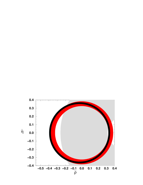
Figure 5: The black annulus shows the region allowed by a measurement of $\overline{Br}\left(\Delta S=0\right)$. The dark shading corresponds to $\overline{Br}_{NL}(B\rightarrow\textit{no charm})$ and the lightly shaded area shows the constraint on $(\overline{\rho},\overline{\eta})$ obtained from $\overline{Br}\left(\Delta S=1\right)$.

 

The figure reveals that $\overline{Br}\left(\Delta S=0\right)$ is a very good observable for the phenomenology of the unitarity triangle. This remains true even if the actual theoretical uncertainty of $20\,\%$ is included. By contrast $\overline{Br}\left(\Delta S=1\right)$ is not very sensitive to $(\overline{\rho},\overline{\eta})$ and thereby yields a much poorer information on the unitarity triangle. Still the center $(\overline{\rho}_{0},0)$ of the circle largely deviates from the origin, so that upper or lower bounds on $\overline{Br}\left(\Delta S=1\right)$ could help to exclude a part of the $(\overline{\rho},\overline{\eta})$-plane allowed by other observables. Also Fig. 5 shows that $\overline{Br}_{NL}(B\rightarrow\textit{no charm})$ is a very useful observable to determine $\sqrt{\overline{\rho}^{2}+\overline{\eta}^{2}}$, once the large $\mu$-dependence of the entries in Tab. 1 is reduced by a complete next-to-leading order calculation of the $\Delta S=1$ decay rates.

The circles from the CP-asymmetries are likewise obtained from (16). Here the measured value of $a_{CP}$ enters the $\overline{\eta}$-coordinate $\overline{\eta}_{0}$ or $\overline{\eta}_{0}^{\prime}$ of the center of the circle and its radius $R_{a}$ or $R_{a}^{\prime}$. For the CP-asymmetries we assume an experimental precision of $20\,\%$ and

$$a_{CP}\left(\Delta S=0\right)\;=\;2.0\,\%, \qquad\qquad a_{CP}\left(\Delta S=1\right)\;=\;-1.0\,\%.$$

 

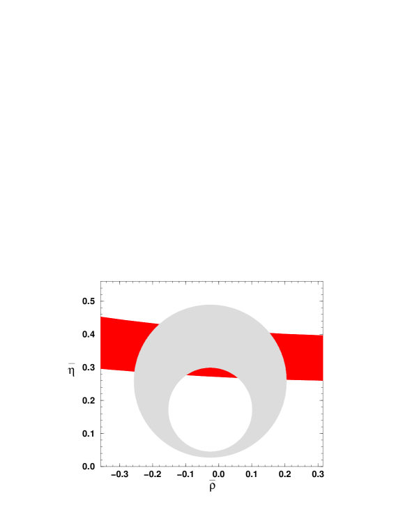
Figure 6: The lightly shaded area shows the constraint stemming from $a_{CP}\left(\Delta S=0\right)$ and the dark shading marks the area allowed from $a_{CP}\left(\Delta S=1\right)$.

 

The results are displayed in Fig. 6. If one switches off the effects of penguin operators, the circle from $a_{CP}\left(\Delta S=0\right)$ touches the $\overline{\rho}$–axis in the point $(0,0)$. The distance of the points on the circle to the origin is therefore proportional to $\sin\gamma$, so that $a_{CP}\left(\Delta S=0\right)$ measures $\sin\gamma/\sqrt{\overline{\rho}^{2}+\overline{\eta}^{2}}$ in this limit as found in (10). The circle from $a_{CP}\left(\Delta S=1\right)$, however, looks totally different: $\overline{\eta}_{0}$ and $R_{a}^{\prime}$ are so large that only a small fraction of the circle can be seen in Fig. 6. $a_{CP}\left(\Delta S=1\right)$ weakly depends on $\overline{\rho}$ and yields good information on $\overline{\eta}$. Hence from Fig. 6 we learn that inclusive CP-asymmetries yield interesting information on the unitarity triangle, which is complementary to the one obtained from other observables in the $B$ system. Alternatively one can multiply $a_{CP}$ with the measured $\overline{Br}$ and obtain $A_{CP}$ of (4), which defines a horizontal straight line in the $(\overline{\rho},\overline{\eta})$-plane (see (15) and (31)).

6 Ten messages from this work

• Inclusive direct CP-asymmetries in charmless $B^{\pm}$–decays are larger than previously believed:

  $$a_{CP}\left(\Delta S=0\right)\;=\;\left(2.0\raisebox{-2.15277pt}{\shortstack[l]{$\scriptstyle+1.2$\\ $\scriptstyle-1.0$}}\right)\%, \quad a_{CP}\left(\Delta S=1\right)\;=\;\left(-1.0\pm 0.5\right)\%.$$

• The dominant contribution to $a_{CP}\left(\Delta S=0\right)$ satisfies

  $$a_{CP}\left(\Delta S=0\right) \propto \frac{\sin\gamma}{\left|V_{ub}/V_{cb}\right|}$$ (60)

  with small and calculable corrections.

• The constraints on the apex $(\overline{\rho},\overline{\eta})$ of the unitarity triangle obtained from a measurement of $a_{CP}\left(\Delta S=0\right)$ and $a_{CP}\left(\Delta S=1\right)$ are circles in the $(\overline{\rho},\overline{\eta})$-plane. These constraints are complementary to the information from other observables in $K$ and $B$ physics.

• Inclusive direct CP-asymmetries are theoretically clean: The uncertainties can be controlled and systematically reduced by higher order calculations.

• The CP-conserving observables $\overline{Br}\left(\Delta S=0\right)$, $\overline{Br}\left(\Delta S=1\right)$ and $\overline{Br}_{NL}(B\rightarrow\textit{no charm})$ define circles in the $(\overline{\rho},\overline{\eta})$-plane centered on the $\overline{\rho}$-axis.

• $\overline{Br}\left(\Delta S=0\right)$ is well suited to determine $|V_{ub}/V_{cb}|$, with little sensitivity to $\gamma$.

• “Double penguin” contributions, which are part of the next-to-next-to-leading order, enhance $\overline{Br}\left(\Delta S=1\right)$ by $13\,\%$.

• The present incomplete next-to-leading order (NLO) result imposes a large $\mu$-dependence on $\overline{Br}\left(\Delta S=1\right)$. Here a calculation of all NLO corrections to penguin operator matrix elements is necessary.

• $\overline{Br}\left(\Delta S=1\right)$ exceeds $\overline{Br}\left(\Delta S=0\right)$ by roughly a factor of two.

• The determination of $|V_{ub}/V_{cb}|$ from $\overline{Br}_{NL}(B\rightarrow\textit{no charm})$ is competitive to the standard method from semileptonic decays, once the NLO calculation mentioned in 8) has been done.

Appendix A Exact formulae

Here we show how the quantities entering sect. 3 and sect. 4 are related to the results of [10]. These expression are useful for readers who are not satisfied with the approximate formulae for $F$, $L_{B}$, $L_{a}$, etc. They are also helpful, if one wants to calculate the branching ratios and CP-asymmetries in extensions of the Standard Model. Then one needs to change the Wilson coefficients entering the $\Gamma_{ij}$’s accordingly.

Now $F$ [14] reads

$$F = \frac{G_{F}^{2}m_{b}^{5}|V_{cb}|^{2}}{64\pi^{3}\Gamma_{tot}}\left(1+\frac{\lambda_{1}}{2m_{b}^{2}}\right)\;=\;\frac{G_{F}^{2}m_{b}^{5}|V_{cb}|^{2}}{64\pi^{3}}\cdot\frac{B_{SL}^{exp}}{\Gamma_{SL}}\left(1+\frac{\lambda_{1}}{2m_{b}^{2}}\right)$$ (61)

$$= \frac{3B_{SL}^{exp}}{f_{1}(x_{c}^{2})\left[1+\alpha_{s}(\mu)/(2\pi)h_{SL}(x_{c})\right]-6\,(1-x_{c}^{2})^{4}\,\lambda_{2}/m_{b}^{2}}$$

in terms of the notation of [10]. Here we have used the common trick to evaluate $\Gamma_{tot}=\Gamma_{SL}/B_{SL}$ via the semileptonic rate and the experimental value of the semileptonic branching ratio $B_{SL}$. This eliminates various uncertainties associated with the theoretical prediction for $\Gamma_{tot}$. The non-perturbative corrections involving the kinetic energy parameter $\lambda_{1}$ has been factored out in (61), because $\lambda_{1}$ cancels in $\overline{Br}$ and $A_{CP}$.

Likewise for the decay rates corresponding to the quark level transition $b\rightarrow q\overline{q}d^{\prime}$, $q=u,d,s$ and $d^{\prime}=d,s$, one has

$$\Gamma_{uu} = t\sum_{i,j=1}^{2}C_{i}C_{j}\left[b_{ij}\left(1-6\frac{\lambda_{2}}{m_{b}^{2}}\right)+\delta b_{ij}+\frac{\alpha_{s}}{4\pi}\,2\,{\rm Re}\,\left[h_{ij}+g_{ij}(0)\right]\right]$$

$$\Gamma_{uc} = t\frac{\alpha_{s}}{2\pi}C_{2}^{2}g_{22}(x_{c})$$

$$\Gamma_{tu} = -2\!\!\!\sum_{\scriptstyle i=1,2\atop\scriptstyle j=3,\ldots 6}\!\!C_{i}C_{j}\left[t\,b_{ij}\left(1-6\frac{\lambda_{2}}{m_{b}^{2}}\right)+t\,\delta b_{ij}+\frac{\alpha_{s}}{4\pi}\left(g_{ij}(0)+tg_{ji}^{*}\left(x_{c}\right)\right)\right]-C_{8}C_{2}\,\frac{\alpha_{s}}{2\pi}\,b_{28}t$$

$$\Gamma_{tc} = -2\!\!\!\sum_{\scriptstyle i=1,2\atop\scriptstyle j=3,\ldots 6}\!\!C_{i}C_{j}\frac{\alpha_{s}}{4\pi}g_{ij}(x_{c})$$

$$\Gamma_{tt} = \sum_{i,j=3,\ldots 6}\!\!C_{i}C_{j}\left[b_{ij}\left(1-6\frac{\lambda_{2}}{m_{b}^{2}}\right)+\delta b_{ij}\right]+\frac{\alpha_{s}}{2\pi}C_{8}\sum_{j=3,\ldots 6}C_{j}b_{j8}$$

$$\Gamma_{cc} = \left(\frac{\alpha_{s}}{4\pi}\right)^{2}C_{2}^{2}\,k_{22}\left(x_{c},x_{c},\frac{\mu}{m_{b}}\right).$$ (62)

Here $t=1$ for $b\rightarrow u\overline{u}d^{\prime}$, while $t=0$ for $b\rightarrow s\overline{s}d^{\prime}$ and $b\rightarrow d\overline{d}d^{\prime}$. The $C_{j}$’s, $\alpha_{s}$ and the loop functions $h_{ij},g_{ij}$ in (62) are understood to be evaluated at the scale $\mu=O(m_{b})$. The $\Gamma_{ij}$’s depend sizeably on $\mu$ and $x_{c}$ as indicated in the approximate formulae in sect. 3. Further they depend on $m_{t}$ and $M_{W}$, this dependence, however, is marginally small. $g_{22}(x_{c})=g(x_{c},\mu/m_{b})$ is the fundamental penguin functions entering all $g_{ij}$’s. For this work we have newly calculated

$$g_{42}\left(x_{c},\frac{\mu}{m_{b}}\right) = g_{62}\left(x_{c},\frac{\mu}{m_{b}}\right)\;=\;n_{f}g\left(0,\frac{\mu}{m_{b}}\right)+g\left(x_{c},\frac{\mu}{m_{b}}\right)+g\left(1,\frac{\mu}{m_{b}}\right),\qquad n_{f}=3,$$

$$g_{32}\left(x,\frac{\mu}{m_{b}}\right) = g\left(0,\frac{\mu}{m_{b}}\right)+g\left(1,\frac{\mu}{m_{b}}\right),\qquad\quad g_{52}\left(x,\frac{\mu}{m_{b}}\right)\;=\;0,$$

$$g\left(1,\frac{\mu}{m_{b}}\right) = -\frac{16}{27}\ln\frac{\mu}{m_{b}}+\frac{98}{8}-\frac{8}{\sqrt{3}}\pi+\frac{32}{81}\pi^{2}.$$ (63)

These quantities correspond to the diagrams of Fig. 4 with $q^{\prime}=u$, $q=u,d,s,c,b$ and the left cut marking the final state $u\overline{u}d$. For the remaining $g_{ij}$’s we refer to [10], where also analytic formulae for $g(x,\mu/m_{b})$ and the $b_{ij}$’s and $h_{ij}$’s [17] can be found. In (62) the leading nonperturbative corrections are also included, the $\delta b_{ij}$’s [18] depend on $\lambda_{2}=0.12$ GeV². The values in (63) correspond to the NDR scheme, the vanishing of $g_{52}$ involves in addition the standard finite renormalization of $Q_{5}$ introduced in [19] and related to the definition of the “effective” coefficient $C_{8}$.

Another new result is $\Gamma_{cc}$ in (62). We have calculated the “double penguin” contribution stemming from the square of Fig. 2 with $q^{\prime}=c$. Although being of order $\alpha_{s}^{2}$ this term is numerically relevant in $\Delta S=1$ decays, because it is proportional to $C_{2}^{2}$ and the tree-level result is CKM suppressed. We have also included $\Gamma_{cc}$ in the $\Delta S=0$ coefficients of (29). Approximately one finds

$$k_{22}\left(x_{c},x_{c},x_{\mu}\right) = \left(1-\frac{r}{6}\right)\big{[}1.52-\>11.5\,(x_{c}-0.3)+\>7\,(x_{c}-0.3)^{2}$$ (64)

$$\quad+\left(1.84-\>5.6\,(x_{c}-0.3)-\>19\,(x_{c}-0.3)^{2}\right)\ln x_{\mu}+0.79\ln^{2}x_{\mu}\big{]}.$$

with $r=0$ for the quark final states $u\overline{u}d$, $u\overline{u}s$, $s\overline{s}d$, $d\overline{d}s$, and $r=1$ for $d\overline{d}d$ and $s\overline{s}s$. The result in (64) receives corrections of order $(x_{c}-0.3)^{3}$ and reproduces $k_{22}$ with an error of 2.6 % for $0.25\leq x_{c}\leq 0.35$ and $0.5\leq\mu/m_{b}\leq 2.0$.

Our results for $\overline{Br}\left(\Delta S=0\right)$ and $\overline{Br}\left(\Delta S=1\right)$ also include the decay rates for $b\rightarrow s\,g$ and $b\rightarrow d\,g$. Here to order $\alpha_{s}$ all $\Gamma_{ij}$’s are zero except for

$$\Gamma_{tt}\left(b\rightarrow s\,g\right)\;=\;\Gamma_{tt}\left(b\rightarrow d\,g\right) = \frac{8}{3}\frac{\alpha_{s}(\mu)}{\pi}C_{8}^{2}.$$

The approximate formulae in (29), (45) and (54) further correspond to $\alpha_{s}(M_{Z})=0.118$ corresponding to $\alpha_{s}(\mu=4.8\mathrm{GeV})=0.216$. The dependence on $\alpha_{s}(M_{Z})$ is non-negligible, but smaller than the $\mu$-dependence.

When calculating $A_{CP}$ for the inclusive $\Delta S=0$ or $\Delta S=1$ final state, we must add the $\Gamma_{ij}$’s for $b\rightarrow u\overline{u}d^{\prime}$, $b\rightarrow s\overline{s}d^{\prime}$ and $b\rightarrow d\overline{d}d^{\prime}$. ${\rm Im}\,\Gamma_{tu}$ contains ${\rm Im}\,g(0)$, which, however, cancels when summing ${\rm Im}\,\Gamma_{tu}$ for the three decay modes $b\rightarrow u\overline{u}d^{\prime}$, $b\rightarrow s\overline{s}d^{\prime}$ and $b\rightarrow d\overline{d}d^{\prime}$, so that $A_{CP}(\Delta S=0)$ and $A_{CP}(\Delta S=1)$ vanish for $x_{c}\geq 1/2$ as required by the CPT theorem. The cancellation takes place when summing the contributions of different cuts of the diagrams in Fig. 4 as found in [2].

One comment is in order here: The terms of order $\alpha_{s}$ in (62) depend on the renormalization scheme. This originates from the fact that when renormalizing $H$ in (1) one already uses the unitarity relation $\xi_{u}+\xi_{c}+\xi_{t}=0$. After using this relation to eliminate, say, $\xi_{c}$ in (2) one finds the coefficients of $|\xi_{u}|^{2}$, $|\xi_{t}|^{2}$ and $\xi_{t}\xi_{u}^{*}$ scheme independent. Consequently by changing the scheme one can shift terms in $A_{CP}$ in (7) from e.g. the term proportional to $\sin\gamma$ to the one multiplying $\sin\beta$. This scheme ambiguity, however, is suppressed by a factor of $C_{3-6}/C_{1,2}$ with respect to the dominant contribution to $a_{CP}$. The constraints on $(\overline{\rho},\overline{\eta})$ derived from $\overline{Br}$ and $a_{CP}$ are scheme independent, of course.

References

- [1] M. Bander, D. Silverman and A. Soni, Phys. Rev. Lett. 43 (1979) 242.
- [2] J.-M. Gérard and W.-S. Hou, Phys. Rev. D43 (1991) 2909.
- [3] H. Simma, G. Eilam and D. Wyler, Nucl. Phys. B352 (1991) 367.
- [4] R. Fleischer, Z. Phys. C 58 (1993) 483.
- [5] L. Wolfenstein, preprint no. NSF-ITP-90-29 (unpublished), and Phys. Rev. D43 (1991) 151.
-
[6]
Yu. Dokshitser and N. Uraltsev,
JETP. Lett. 52 (1990) 509.
N. Uraltsev, hep-ph/9212233. - [7] M. Beneke, G. Buchalla and I. Dunietz, Phys. Lett. B393 (1997) 132.
- [8] M. Daoudi for the SLD Collaboration (K. Abe et al.), hep-ex/9712031, talk at International Europhysics Conference on High-Energy Physics (HEP 97), 19-26 Aug 1997, Jerusalem.
- [9] T.E. Browder, A. Datta, X.-G. He and S. Pakvasa, hep-ph/9705320.
- [10] A. Lenz, U. Nierste and G. Ostermaier, Phys. Rev. D56 (1997) 7228.
- [11] A. J. Buras, M. E. Lautenbacher, G. Ostermaier, Phys. Rev. D50 (1994) 3433.
-
[12]
S. Herrlich and U. Nierste, Nucl. Phys. B419 (1994) 292.
S. Herrlich and U. Nierste, Nucl. Phys. B476 (1996) 27.
S. Herrlich and U. Nierste, Phys. Rev. D52 (1995) 6505.
U. Nierste, hep-ph/9609310, Proceedings of the Workshop on K Physics, Orsay, 30 May- 4 June 1996, ed. L. Iconomidou-Fayard, 163-170, Editions Frontieres 1997. - [13] A. J. Buras, M. Jamin and P. H. Weisz, Nucl. Phys. B347 (1990) 491.
- [14] Y. Nir, Phys. Lett. B221 (1989) 184.
- [15] M. Neubert, hep-ph/9801269, plenary talk at International Europhysics Conference on High-Energy Physics (HEP 97), 19-26 Aug 1997, Jerusalem.
- [16] CLEO coll. (T.E. Coan et. al.), hep-ex/9710028.
-
[17]
G. Altarelli, G. Curci, G. Martinelli and S. Petrarca,
Nucl. Phys. B187 (1981) 461.
G. Buchalla, Nucl. Phys. B391 (1993) 501.
E. Bagan, P. Ball, V.M. Braun and P. Gosdzinsky, Nucl. Phys. B432 (1994) 3. - [18] I.I. Bigi, B. Blok, M. Shifman and A. Vainshtein, Phys. Lett. B323 (1994) 408.
- [19] M. Ciuchini, E. Franco, G. Martinelli, L. Reina and L. Silvestrini, Phys. Lett. B316 (1993) 127.