SAGA-HE-129-98 January 10, 1998

 

* Email: kumanos@cc.saga-u.ac.jp.

Information on his research is available at

http://www.cc.saga-u.ac.jp/saga-u/riko/physics/quantum1/structure.html.

to be published in Genshikaku Kenkyu

      

      

      

      

      

1 Introduction

Internal spin structure of the proton has been investigated extensively for the last ten years. Although the proton spin is no more considered at the stage of “crisis”, the clear explanation is still far from the final one. In particular, there is essentially no information on sea-quark and gluon polarizations. Furthermore, parton’s angular momenta may have influence on the issue. In order to clarify these problems, the RHIC-Spin project was proposed [1]. Obtained data at the RHIC facility should be able to pin down how the proton spin consists of internal constituent spins.

The RHIC facility will provide us fruitful information on the proton spin structure. In order to understand the situation of proton-spin studies and also to explore possible RHIC-Spin physics, we established a Japanese working group on parametrization of polarized parton distributions [2]. For the time being, the purpose is to obtain the optimum parton distributions for explaining existing polarized experimental data. Our study is still at the preliminary stage [3]. The parametrization of unpolarized parton distributions has been well studied since 1980’s. It is also fortunate that abundant experimental data are available through various reactions in the unpolarized case. Accurate distributions are now known from very small $x$ to relatively large $x$. The same parametrization study can be done for the longitudinally polarized parton distributions because many experimental data are now available for the structure function $g_{1}$ [4].

The proton spin is so far investigated mainly in the longitudinally polarized structure function $g_{1}$. However, it is also interesting to test it by transversely polarized structure functions. In particular, the leading-twist structure function $h_{1}$ should be an interesting topic. It is expected to be measured in the transversely polarized Drell-Yan processes at RHIC. We should try to understand the properties of $h_{1}$ before the experimental data are taken. The transversity distribution is an unexplored subject experimentally. If future experimental data on $h_{1}$ are much different from theoretical expectation, a new field of spin physics could be developed.

We have been working on calculation of the next-to-leading-order (NLO) anomalous dimensions for $h_{1}$ and also on numerical solution of its evolution equation [5]. We also studied the numerical solution of the Dokshitzer-Gribov-Lipatov-Altarelli-Parisi (DGLAP) evolution equations for the longitudinally polarized distributions [6]. In general, parton distributions are provided at $Q^{2}\sim O$(1 GeV²) and experimental data are taken at different $Q^{2}$ points. Therefore, our studies on the numerical solution should be useful for extracting information on the polarized parton distributions from polarized RHIC data.

The major audience are traditional nuclear physicists at this symposium, so that we first discuss how each unpolarized parton distribution is obtained from various experimental data in section 2. The section 3 is devoted to the activities of the RHIC-Spin-J working group. A brief outline of the parametrization project is explained. We discuss the numerical solution of the DGLAP $Q^{2}$ evolution equations for the longitudinally polarized and transversity distributions in section 4. The summary is given in section 5.

2 Extraction of parton distributions

Nucleon substructure has been investigated through various high-energy experiments. For example, electron or muon deep inelastic scattering has been used. Its unpolarized cross section is related to two structure functions $F_{1}$ and $F_{2}$. They depend in general on two kinematical variables $Q^{2}=-q^{2}$ and $x=Q^{2}/2p\cdot q$ where $q$ is the virtual photon momentum and $p$ is the nucleon momentum. It is known that the structure functions are almost independent of $Q^{2}$, which is referred to as Bjorken scaling. It indicates that the photon scatters on structureless objects, which are called partons. They are now identified with quarks and gluons. Because the variable $x$ is the light-cone momentum fraction carried by the struck quark, it is possible to extract quark-momentum distributions from the $F_{2}$ data.

The $x$ dependence of the parton distributions are expressed by several parameters at fixed $Q^{2}$ (=$Q_{0}^{\,2}$): for example $x\,f_{i}(x,Q_{0}^{\,2})\,=\,A_{i}\,\eta_{i}\,x^{\alpha_{i}}\,(1-x)^{\beta_{i}}\,(1+\gamma_{i}\,x+\rho_{i}\,\sqrt{x})$, and the parameters are optimized so as to explain the existing data. There are abundant experimental data on unpolarized parton distributions such as those taken by electron/muon/neutrino deep inelastic scattering, Drell-Yan, and direct-photon process. With these experimental data, accurate parton distributions are now known although there are still detailed issues on the distributions at large $x$ and very small $x$. The updated information on the optimum parton distributions is given at http://durpdg.dur.ac.uk/HEPDATA/HEPDATA.html and http://www.phys.psu.edu/$\tilde{\ }$cteq. The major parametrization groups are CTEQ (Coordinated Theoretical/Experimental Project on QCD Phenomenology and Tests of the Standard Model), GRV (Glück, Reya, and Vogt), and MRS (Martin, Roberts, and Stirling). In this section, we introduce how the parton distributions are extracted from various experimental data for a novice.

2.1 Valence-quark distributions

The parton distributions are usually separated into valence-quark, sea-quark, and gluon distributions. The valence-quark distribution is defined by the difference between quark and antiquark distributions: $q_{v}\equiv q-\bar{q}$. It can be obtained by analyzing neutrino deep inelastic data. The cross section of the neutrino reaction ${\nu}_{\mu}+p\rightarrow{\mu}^{-}+X$ is expressed as $d\sigma\propto\ell^{\mu\nu}W_{\mu\nu}$ with the lepton tensor $\ell^{\mu\nu}$ and hadron tensor $W_{\mu\nu}$ [7]. The lepton tensor is calculated as

$${\ell}^{\mu\nu}= {\overline{\sum_{spins}}}\,\overline{u}(k){\gamma}^{\mu}(1-{\gamma}_{5})u(k^{\prime})\cdot\rm\overline{u}(k^{\prime}){\gamma}^{\nu}(1-{\gamma}_{5})u(k)$$

$$= \,2\left[{\,{k}^{\mu}{k^{\prime}}^{\nu}+{k}^{\nu}{k^{\prime}}^{\mu}-{g}^{\mu\nu}k\cdot k^{\prime}+i{\varepsilon}^{\mu\nu\rho\sigma}{k}_{\rho}{k^{\prime}}_{\sigma}\,}\right]\ \ .$$ (2.1)

Because of the axial vector term $\gamma^{\mu}\gamma_{5}$ in the neutrino reaction, there appears the antisymmetric term ${\varepsilon}^{\mu\nu\rho\sigma}$, which does not exist in the electron scattering. Due to the existence of this term in the lepton tensor, the hadron tensor could also have an antisymmetric one:

$$\!\!\!\!{W}_{\mu\nu}=-\,W_{1}\,({g}_{\mu\nu}-\frac{{q}_{\mu}{q}_{\nu}}{{q}^{2}})+\,W_{2}\,\frac{1}{{M}^{2}}\,({p}^{\mu}-\frac{p\cdot q}{{q}^{2}}{q}^{\mu})({p}^{\nu}-\frac{p\cdot q}{{q}^{2}}{q}^{\nu})-\frac{i}{M}\,W_{3}\,{\varepsilon}_{\mu\nu\rho\sigma}\,{p}^{\rho}\,{q}^{\sigma}\,.$$ (2.2)

From these expressions, the cross section becomes

$$\!\!\!\!\frac{{d\sigma}^{\pm}}{d{E}^{{}^{\prime}}d\Omega}=\frac{{G}_{F}^{2}\,{E^{\prime}}^{2}}{2{\pi}^{2}(1+{Q}^{2}/{M}_{W}^{2}{)}^{2}}{\bigg{[}}2{W}_{1}(\nu,{q}^{2})\,{\sin}^{2}\frac{\theta}{\rm 2}+{W}_{2}(\nu\rm,{q}^{2})\,{\cos}^{2}\frac{\theta}{2}\mp\frac{E+E^{\prime}}{M}{W}_{3}\,{\sin}^{2}\frac{\theta}{2}{\bigg{]}}\,,$$ (2.3)

where $\pm$ indicates W^± exchange processes. The new term with $W_{3}$ is associated with the parity violation, and it is given by the difference between the left and right cross sections for the W: ${W}_{3}\ \propto{\sigma}_{{}_{L}}-{\sigma}_{{}_{R}}$. Instead of $W_{3}$, the scaling function ${F}_{3}=\nu{\rm W}_{\rm 3}$ is usually used. Because of the ${\sigma}_{{}_{L}}-{\sigma}_{{}_{R}}$ property, the structure function $F_{3}$ is given as the quark $-$ antiquark distribution form: ${F}_{3}^{\nu\rm p}=2\,(d+s-\overline{u}-\overline{c})$ and ${F}_{3}^{\overline{\nu}p}=2\,(u+c-\overline{d}-\overline{s})$. Hence, we have

$${F}_{3}^{\ p}=\frac{{F}_{3}^{\nu\rm p}+{F}_{3}^{\overline{\nu}p}}{2}={u}_{v}+{d}_{v}\ ,$$ (2.4)

if $s=\overline{s}$ and $c=\overline{c}$. It is known theoretically, for example, that the $s$ distribution is not exactly equal to the $\bar{s}$. However, because the corrections are expected to be small, the valence quark distribution $u_{v}+d_{v}$ can be extracted from the neutrino data.

2.2 Sea-quark distributions

The $F_{2}$ structure function can be used for extracting both valence and sea quark distributions. It is given by quark distributions weighted by the square of their charges:

$$F_{2}(x,Q^{2})=\sum_{i}e_{i}^{\,2}\,x\,[\,q(x,Q^{2})\,+\,\bar{q}(x,Q^{2})\,]\ ,$$ (2.5)

in the leading order. Because it is dominated by the valence distributions at medium and large $x$ regions, $q_{v}$ can be obtained directly from the $F_{2}$ data in these regions. The $F_{2}$ structure function at small $x$ is , on the other hand, dominated by the sea-quark distributions. Therefore, $q_{sea}$ ($=\bar{q}$) can be obtained in the small $x$ region from the $F_{2}$ data.

The other method is to use Drell-Yan processes ${p}_{1}+{p}_{2}\rightarrow{\mu}^{+}{\mu}^{\bf-}+X$. Its cross section is described by the $q\bar{q}$ annihilation processes:

$$s\,\frac{d\sigma}{d\sqrt{\tau}\,dy}=\frac{8\,\pi\,{\alpha}^{2}}{9\,\sqrt{\tau}}\,\sum\limits_{\rm i}{e}_{i}^{\,2}\,[\,q({x}_{1},{Q}^{2})\,\overline{q}({x}_{2},{Q}^{2})+\overline{q}({x}_{1},{Q}^{2})\,q({x}_{2},{Q}^{2})\,]\ ,$$ (2.6)

where $Q^{2}$ is the dimuon mass squared: $Q^{2}=m_{\mu\mu}^{2}$, and $\tau$ is given by $\tau=m_{\mu\mu}^{2}/s=x_{1}x_{2}$. The rapidity $y$ is defined by dimuon longitudinal momentum $P_{L}^{*}$ and dimuon energy $E^{*}$ in the c.m. system: $y=(1/2)ln[(E^{*}+P_{L}^{*})/(E^{*}-P_{L}^{*})]$. The momentum fractions $x_{1}$ and $x_{2}$ can be written by these kinematical variables: $x_{1}=\sqrt{\tau}e^{y}$ and $x_{2}=\sqrt{\tau}e^{-y}$. In the large $x_{{}_{F}}=x_{1}-x_{2}$ region, namely at large $x_{1}$, the cross section is dominated by the projectile-quark annihilation process with an target antiquark: $d\sigma\propto{q}_{v}({x}_{1})\overline{q}({x}_{2})$ because of $\bar{q}(x_{1})<<1$. This equation indicates that the sea-quark distribution $\overline{q}({x}_{2})$ can be measured if the valence-quark distributions in the projectile are known.

In these days, the details are investigated for the sea-quark distributions. Neutrino-induced dimuon events are interpreted by the charm-production process: $\nu_{\mu}+(s,d)\rightarrow$$\mu^{-}+c$ then $c\rightarrow s+\mu^{+}+\nu_{\mu}$, so that the strange quark distribution can be extracted from the data. It is now known $s+\bar{s}\approx 0.5\,(\bar{u}+\bar{d})$ at $Q^{2}\approx 20$ GeV². Furthermore, flavor asymmetry in light antiquark distributions was also found by the Gottfried-sum-rule violation and by the p-n asymmetry in the Drell-Yan experiments [8].

2.3 Gluon distribution

There are two major methods for finding the gluon distribution. The first one is to use scaling violation data of the $F_{2}$ structure function, and the second is to use direct photon data. We mentioned that the structure functions are almost independent of $Q^{2}$. However, it is known that they vary as a function of $ln\,Q^{2}$ even though it is small. This is called scaling violation. The $Q^{2}$ dependence is described by the DGLAP evolution equations, which are the coupled integrodifferential equations:

$$\frac{\partial}{\partial\ln Q^{2}}\,\left(\begin{array}[]{c}{q}_{s}(x,Q^{2})\\ g(x,Q^{2})\end{array}\right)=\frac{\alpha_{s}(Q^{2})}{2\pi}\,\left(\begin{array}[]{cc}P_{qq}(x,Q^{2})&P_{qg}(x,Q^{2})\\ P_{gq}(x,Q^{2})&P_{gg}(x,Q^{2})\\ \end{array}\right)\otimes\left(\begin{array}[]{c}{q}_{s}(x,Q^{2})\\ g(x,Q^{2})\end{array}\right)\ ,$$ (2.13)

where $q_{s}=\sum_{i}(q_{i}+\bar{q}_{i})$ is the singlet quark distribution. The convolution integral $\otimes$ is defined by $f(x)\otimes g(x)=\int^{1}_{x}f(x/y)\,g(y)\,dy/y$. Each term describes the process that a parton $p_{j}$ with the nucleon’s momentum fraction $y$ splits into a parton $p_{i}$ with the momentum fraction $x$ and another parton. The splitting function $P_{p_{i}p_{j}}(z)$ determines the probability that such a splitting process occurs and the $p_{j}$-parton momentum is reduced by the fraction $z$. The $Q^{2}$ dependence of the quark distribution is affected by the gluon distribution through the splitting function. In the small $x$ region, the right-hand sides of the evolution equations are dominated by the gluon terms. Therefore, the gluon distribution can be extracted from the $Q^{2}$ dependent data of $F_{2}$. To be explicit, the $Q^{2}$ dependence of $F_{2}$ is approximately proportional to the gluon distribution: $\partial F_{2}(x,Q^{2})/\partial(\ln\,Q^{2})\approx 10\,\alpha_{s}G(2x,Q^{2})/(27\,\pi)$.

Figure 1: QCD Compton process.

The second method is to use direct photon data. The leading-order cross section is calculated by the QCD Compton scattering ($gq\rightarrow\gamma q$) and annihilation ($\bar{q}q\rightarrow\gamma g$) processes. Because the gluon distribution is involved in the Compton process in Fig. 1, it is possible to extract it from the experimental data. The quark and antiquark distributions are also involved in the reaction; however, they are relatively well known from deep inelastic scattering data. It is also possible to isolate the annihilation contribution by using both $pp$ and $p\bar{p}$ reaction data. From the scaling violation and direct photon data, the gluon distribution in the nucleon is now well known except for the small and large $x$ regions. The large $x$ distribution is particularly important for judging whether the CDF jet production data could suggest “subquark” structure. It is desirable to measure the gluon distribution in the $x$ region, $x\sim 0.5$, directly by some kind of experiments. On the other hand, the small $x$ distribution is not well fixed as it is obvious from the R1, R2, R3, and R4 type distributions in the MRS parametrizations [9]. It is partly because a wide range of $Q^{2}$ data is not available in the structure function $F_{2}$. These $x$ regions of the gluon distribution should be studied experimentally in future.

3 Activities of the RHIC-Spin-J working group

With the completion of the RHIC facility in mind, we created a working group within Japan for studying possible spin physics at RHIC. We have a monthly meeting at Riken among related theorists and experimentalists. One of the activities is to study the parametrization of the polarized parton distributions. Even though the study is still preliminary, we discuss an outline of our efforts.

The parametrization of the unpolarized distributions has been studied extensively as discussed in the previous section. On the other hand, the polarized distributions are not well known yet due to lack of a variety of experimental data. However, several sets of longitudinally polarized distributions are proposed by analyzing the $g_{1}$ structure functions for the proton, deuteron, and ${}^{3}He$ [4]. With stimulation of these studies and recent polarized measurements, we initiated a parametrization project within Japan [2]. Because this is a part of the Japanese RHIC-Spin activities, the ultimate purpose is to use our studies for the RHIC-Spin experiments. At this stage, the group consists of Y. Goto, N. Hayashi, M. Hirai, H. Horikawa, S. Kumano, M. Miyama, T. Morii, N. Saito, T.-A. Shibata, E. Taniguchi, and T. Yamanishi. For the time being, this collaboration intends to obtain optimum polarized parton distributions for explaining all the available experimental data. We have been working for a year, and we should be able to complete our first work in a few months. It includes complete NLO analyses of the $g_{1}$ structure functions. The obtained distributions will be used for experimental studies at RHIC. Furthermore, once new experimental results are obtained at RHIC or at other facilities, we try to reanalyze the data for getting updated distributions.

We work in three subgroups: data analysis, parametrization, and $Q^{2}$ evolution. The data analysis subgroup (Y. Goto, N. Hayashi, N. Saito, T.-A. Shibata, and E. Taniguchi) collects all the available experimental data and investigate their systematic uncertainties. At this stage, the data come from measurements of the $g_{1}$ structure functions for the proton and “neutron”. The parametrization group (T. Morii, H. Horikawa, and T. Yamanishi) tries to understand the meaning of obtained parameter values. They also spend much time for running the fitting program. The third subgroup (M. Hirai, S. Kumano, and M. Miyama) contributes to the $Q^{2}$ evolution program. The evolution equations are coupled integrodifferential equations with complicated splitting functions. This subgroup develops an efficient program for numerical solution of the evolution equations. Our parametrization studies were reported by N. Saito at the spring JPS meeting in 1997 [3]. Recent studies were also reported by M. Hirai and T. Yamanishi at this meeting [3].

The distributions are set up at certain $Q^{2}$ ($\equiv Q_{0}^{\,2}$). Experimental data are taken, in general, at different $Q^{2}$ points. The DGLAP evolution equations are used for calculating the distribution variations from $Q_{0}^{\,2}$ to experimental $Q^{2}$. The DGLAP equations assume perturbative QCD, so that both $Q_{0}^{\,2}$ and $Q^{2}$ have to be in the perturbative region. The $Q_{0}^{\,2}$ is taken typically in the 1$-$4 GeV² region except for the GRV distributions, where small $Q_{0}^{\,2}\,(\sim$0.3 GeV${}^{2})$ is chosen. If it is possible, it is desirable to take very large $Q_{0}^{\,2}$ where perturbative QCD is certainly valid. However, because many data are taken in the $Q^{2}$ region 1 GeV${}^{2}<Q^{2}<$a few dozen GeV², we end up taking relatively small $Q_{0}^{\,2}$ at this stage.

We provide polarized parton distributions with a number of parameters at $Q_{0}^{\,2}$, for example at 1 GeV². These parameters are determined by fitting the existing experimental data on $A_{1}$, which is given by

$$A_{1}\cong\frac{g_{1}(x,Q^{2})}{F_{1}(x,Q^{2})}=g_{1}(x,Q^{2})\,\frac{2\,x\,(1+R)}{F_{2}(x,Q^{2})}\ ,$$ (3.1)

where the $F_{1}$ structure function is related to the $F_{2}$ structure function and the $R$ function by $R=(F_{2}-2xF_{1})/(2xF_{1})$. The $g_{1}$ structure function is calculated by the convolution integral of the polarized parton distributions with the coefficient functions:

$${g}_{1}(x,{Q}^{2})=\frac{1}{2}\,\sum\limits_{q}e_{q}^{2}\,\bigg{\{} \int_{x}^{1}\frac{dy}{y}\,\Delta C_{q}(x/y,Q^{2})\,[\,\Delta q(y,Q^{2})\,+\,\Delta\overline{q}(y,Q^{2})\,]$$

$$+ \int_{x}^{1}\frac{dy}{y}\,\Delta C_{g}(x/y,Q^{2})\,\Delta g(y,Q^{2})\,\bigg{\}}\ .$$ (3.2)

It is not a good idea to analyze the published $g_{1}$ values directly because it is often assumed in the experimental analyses that $A_{1}$ is $Q^{2}$ independent. As it is obvious from the results in the next section (see Figs. 5 and 5), it is not a correct assumption. However, considering the present experimental errors, one cannot help using the assumption. In our analysis, the asymmetry $A_{1}$ data are analyzed without using the $Q^{2}$ independent assumption. We investigated various functional forms of the initial distributions; however, the studies have not been completed yet. For example, the $x$ dependence is given as $x\,\Delta f_{i}(x,Q_{0}^{\,2})\,=\,A_{i}\,\eta_{i}\,x^{\alpha_{i}}\,(1-x)^{\beta_{i}}\,(1+\gamma_{i}\,x+\rho_{i}\,\sqrt{x})$ in the analysis of Gehrmann and Stirling (GS). The $F_{2}$ structure function is given in the similar way as

$$F_{2}(x,Q^{2})=\sum\limits_{q}e_{q}^{2}\,x\,\bigg{\{} \int_{x}^{1}\frac{dy}{y}\,C_{q}(x/y,Q^{2})\,[\,q(y,Q^{2})+\overline{q}(y,Q^{2})\,]$$

$$+ \int_{x}^{1}\frac{dy}{y}\,C_{g}(x/y,Q^{2})\,g(y,Q^{2})\,\bigg{\}}\ .$$ (3.3)

Figure 2: Fitting results (preliminary) [3].

Because the unpolarized distributions are not studied by our group at least at this stage , we take distributions $f_{i}(x,Q_{0}^{\,2})$ by CTEQ, GRV, or MRS. With these preparations, we are ready for the optimization. We compare the theoretical asymmetries $A_{1}$ with the experimental data and minimize

$$\chi^{2}\,=\,\sum\limits\frac{(A_{1}^{data}\,-\,A_{1}^{calc})^{2}}{(\sigma_{A_{1}^{data}})^{2}}$$ (3.4)

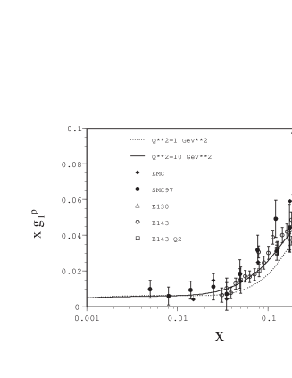
by using the CERN subroutine MINUIT. Because the only information comes from the longitudinally polarized structure function $g_{1}$, the polarized sea-quark and gluon distributions are not well determined at this stage. We tried to find the optimum parameter set by fitting the data with the $Q^{2}$ evolution effects. In Fig. 2, our preliminary fitting results are shown with various experimental data for $g_{1}^{\,p}$ [3]. The dotted curve is the initial distribution at $Q^{2}$=1 GeV², and the solid one is the distribution at $Q^{2}$=10 GeV². We are still working on obtaining the best fit.

We have been studying the parametrization for almost a year. The leading order (LO) fitting program was completed a half year ago, and we try to understand physics meaning of the obtained parameters. On the other hand, we completed the NLO program and the NLO analysis is in progress. We should be able to report our results within a few months.

4 Numerical solution of longitudinal and transversity $Q^{2}$ evolution equations

The DGLAP evolution equations are frequently used in theoretical and experimental analyses. In fact, our evolution program is used in the parametrization studies in the last section. The evolution equations are coupled integrodifferential equations with complex splitting functions in the NLO case. It is, therefore, important to create a computer program to solve them accurately and to publish it so that other people could use the subroutine. We have been working on this topic for several years [5, 6, 10]. In this section, we report the numerical solution of the $Q^{2}$ evolution equations for the longitudinally polarized and transversity distributions.

The longitudinal DGLAP equations are given in the similar way with the unpolarized ones. The nonsinglet equation is

$$\frac{\partial}{\partial\ln Q^{2}}\,\Delta\widetilde{q}_{{}_{NS}}(x,Q^{2})\ =\frac{\alpha_{s}(Q^{2})}{2\pi}\,\Delta\widetilde{P}_{q^{\pm},{NS}}(x)\otimes\Delta\widetilde{q}_{{}_{NS}}(x,Q^{2})\ ,$$ (4.1)

where $\Delta\widetilde{q}_{{}_{NS}}=x\Delta q_{{}_{NS}}$ is a longitudinally polarized nonsinglet parton distribution with $\Delta q=q_{\uparrow}-q_{\downarrow}$. The parton distribution and the splitting function multiplied by $x$ are denoted as $\widetilde{f}(x)=xf(x)$. The function $\Delta\widetilde{P}_{q^{\pm},{NS}}=x\Delta P_{q^{\pm},{NS}}$ is the polarized nonsinglet splitting function. The notation $q^{\pm}$ in the splitting function indicates a $\Delta q^{+}=\Delta q+\Delta\bar{q}$ or $\Delta q^{-}=\Delta q-\Delta\bar{q}$ distribution type. The singlet $Q^{2}$ evolution is described by the coupled integrodifferential equations due to the gluon participation:

$$\frac{\partial}{\partial\ln Q^{2}}\left(\begin{array}[]{c}\Delta\widetilde{q}_{s}(x,Q^{2})\\ \Delta\widetilde{g}(x,Q^{2})\end{array}\right)=\frac{\alpha_{s}(Q^{2})}{2\pi}\left(\begin{array}[]{cc}\Delta\widetilde{P}_{qq}(x,Q^{2})&\Delta\widetilde{P}_{qg}(x,Q^{2})\\ \Delta\widetilde{P}_{gq}(x,Q^{2})&\Delta\widetilde{P}_{gg}(x,Q^{2})\\ \end{array}\right)\otimes\left(\begin{array}[]{c}\Delta\widetilde{q}_{s}(x,Q^{2})\\ \Delta\widetilde{g}(x,Q^{2})\end{array}\right)\!.$$ (4.8)

The singlet quark distribution is defined by $\Delta\widetilde{q}_{s}\equiv\sum_{i}^{N_{f}}x\,\Delta q_{i}^{+}$ where $i$ is the flavor, and $\Delta\widetilde{g}(x,Q^{2})$ is the gluon distribution $\Delta\widetilde{g}=x\,(g_{+1}-g_{-1})$. The LO and NLO [11] evolution equations are described by the above integrodifferential equations. The differences between the LO and NLO are contained in the running coupling constant $\alpha_{s}$ and in the splitting functions. The renormalization scheme is the modified minimal subtraction scheme ($\overline{MS}$) in the NLO analysis.

In addition to the unpolarized and longitudinally polarized evolution equations, the NLO evolution for the transversity distribution was completed recently [12]. The transversity distribution is denoted as $h_{1}$, $\delta q$, or $\Delta_{{}_{T}}q$. Throughout this paper, the notation $\Delta_{{}_{T}}q$ is used. Because the gluon does not couple due to the chiral-odd nature of $\Delta_{{}_{T}}q$, the evolution is described by a single integrodifferential equation,

$$\frac{\partial}{\partial\ln Q^{2}}\,\Delta_{{}_{T}}q^{\pm}(x,Q^{2})\,=\frac{\alpha_{s}(Q^{2})}{2\pi}\,\Delta_{{}_{T}}P_{q^{\pm}}(x)\otimes\Delta_{{}_{T}}q^{\pm}(x,Q^{2})\ .$$ (4.9)

Numerical analysis of the transversity evolution is simple in the sense that it is given only by the “nonsinglet” type equation.

The longitudinally polarized and transversity distributions will be measured at RHIC by polarized p+p reactions. However, they are measured at different $Q^{2}$ points. In order to extract information on the polarized parton distributions, an accurate program for solving the evolution equations should be developed. We have been studying on this topic, and the following discussions are based on the numerical results in Refs. [5, 6]. We simply divide the variables $Q^{2}$ and $x$ into small steps. Then, the integration and differentiation are defined by

$$\frac{df(x)}{dx} =\frac{f(x_{m+1})-f(x_{m})}{\delta x_{m}}\ ,$$ (4.10)

$$\int f(x)\ dx =\sum_{m=1}^{N_{x}}\delta x_{m}\,f(x_{m})\ .$$ (4.11)

With these replacements, the evolution equations could be solved rather easily. We call this method a “brute-force” method [6]. The better method, by means of convergence and computing time, was studied in Ref. [5] by changing the $x$ integration for the Simpson’s method. As the step number becomes larger, the numerical accuracy becomes better. We obtain the numerical accuracy better than 1% in the $x$ region $10^{-8}<x<0.8$ with two hundred $Q^{2}$ steps and one thousand $x$ steps in the brute-force method and with fifty $Q^{2}$ steps and five hundred $x$ steps in the Simpson’s method.

Figure 3: $Q^{2}$ evolution results for $g_{1}^{p}$ [6].

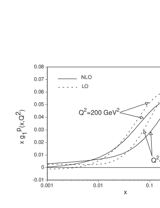
We show evolution results of the longitudinally polarized parton distributions and transversity distributions by using the developed programs, BFP1 [6] and H1EVOL [5]. First, the longitudinal evolution is discussed. The initial distributions are the GS set-A distributions at $Q^{2}$=4 GeV². The evolution results are shown in Fig. 3. The same GS-A distributions are assumed for the LO and NLO cases, so that the differences between the LO and NLO curves at $Q^{2}$=4 GeV² are solely due to the NLO coefficient functions. The $xg_{1}$ distributions are evolved to those at $Q^{2}$=200 GeV². They increase at small $x$ and decrease at large $x$. The major differences between the LO and NLO distributions at $Q^{2}$=200 GeV² are also due to the coefficient functions.

Figure 4: $Q^{2}$ dependence of $A_{1}^{p}$ is calculated in the LO (dashed curve) and NLO (solid curve) cases at $x=0.035$ [6].

Figure 5: Spin asymmetry $A_{1}^{p}$ at $x=0.25$ [6].

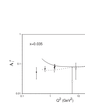
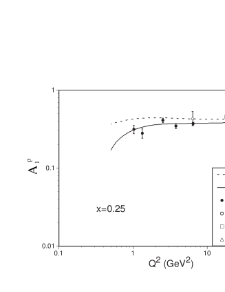
In Fig. 5, our evolution curves at $x$=0.035 are shown with the asymmetry $A_{1}$ data. The dashed and solid curves indicate the LO and NLO evolution results, respectively. In the large $Q^{2}$ region, both results are almost the same; however, they differ significantly at small $Q^{2}$ particularly in the region $Q^{2}<\,$2 GeV². In the medium $x$ region ($x$=0.25), the difference becomes larger again at small $Q^{2}$ as shown in Fig. 5. From these figures, we find that the asymmetry has $Q^{2}$ dependence although it is not large. People used to assume that the asymmetry is independent of $Q^{2}$ by neglecting the $Q^{2}$ evolution difference between $g_{1}$ and $F_{1}$ in analyzing the experimental data. We find clearly that it is not the case. For a precise analysis, the $Q^{2}$ dependence in the asymmetry has to be taken into account.

Next, we discuss the transversity evolution $\Delta_{{}_{T}}q$. It has a chiral-odd property so that it cannot be found in inclusive deep inelastic electron scattering. It is expected to be measured in the RHIC-Spin project by the transversely polarized Drell-Yan processes. The distribution $\Delta_{{}_{T}}q$ is the probability to find a quark with spin polarized along the transverse spin of a polarized proton minus the probability to find it polarized oppositely. There is a problem in studying the transversity evolution in the sense that the input distribution is not available. However, it is known within quark models that the transversity distributions are almost the same as the corresponding longitudinally polarized distributions. Therefore, we may use a longitudinal distribution as an input transversity distribution at small $Q^{2}$, where the quark models would be valid. This consideration is fine at $Q^{2}\sim\Lambda_{QCD}^{\,2}$. On the other hand, the perturbative QCD cannot be used at such a small $Q^{2}$. In the following numerical analysis, we simply assume $\Delta q=\Delta_{{}_{T}}q$ at relatively large $Q^{2}$ (=$\,4$ GeV²) by taking the GS-A distributions as the input.

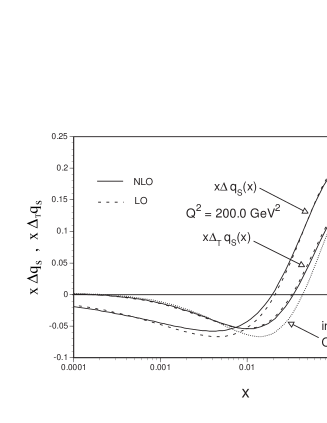
We show the evolution results of two distributions, the singlet distribution $x\sum_{i}(\Delta_{{}_{T}}q+\Delta_{{}_{T}}\bar{q})$ and the valence distribution $x(\Delta_{{}_{T}}u_{v}+\Delta_{{}_{T}}d_{v})$. First, the singlet evolution is shown in Fig. 7. The same GS-A distribution is assumed for the transversity and longitudinally-polarized parton distributions at $Q^{2}$=4 GeV². The initial distribution is shown by the dotted curve. It is evolved to the distributions at $Q^{2}$=200 GeV² by the transverse or longitudinal evolution equation. The transversity NLO effects increase the evolved distribution at medium-large $x$ and also at small $x$ ($<$0.01), and they decrease the distribution in the intermediate $x$ region ($0.01<x<0.1$). The transversity evolution differs significantly from the longitudinal one either in the LO case or in the NLO. The evolved transversity distribution $\Delta_{{}_{T}}q_{s}$ is significantly smaller than the longitudinal one $\Delta q_{s}$ in the region $x\sim 0.1$. The magnitude of $\Delta_{{}_{T}}q_{s}$ itself is also smaller than that of $\Delta q_{s}$ at very small $x$ ($<0.07$).

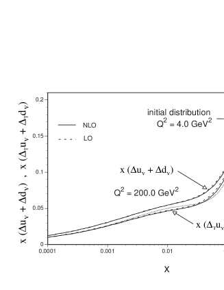
Second, the evolution of the valence-quark distribution is shown in Fig. 7. The evolution calculations are done in the same way. The dotted curve is the initial distribution, and the evolved distributions are solid and dashed curves. The evolved transversity distributions are significantly smaller than the longitudinally polarized ones, in particular at small $x$.

Figure 6: The singlet transversity evolution results are compared with those of longitudinally polarized singlet distribution [5].

Figure 7: Evolution results of the valence-quark transversity distribution $x(\Delta_{{}_{T}}u_{v}+\Delta_{{}_{T}}d_{v})$ are compared with those of the longitudinally polarized one [5].

We have created the useful computer programs, BFP1 and H1EVOL, for solving the DGLAP evolution equations for the longitudinally polarized parton distributions and for the transversity distributions. They should be convenient for theoretical and experimental researchers, who are involved in high-energy spin physics. Our program can be obtained from M. Hirai, SK, or M. Miyama upon email request. For the details, the reader may look at the WWW home page: http://www.cc.saga-u.ac.jp/saga-u/riko/physics/quantum1/program.html.

5 Summary

Since the Riken decided to join the RHIC-Spin project, we have been studying the physics aspects of the project. In particular, the parametrization of polarized parton distributions has been investigated among the members. For general audience at this symposium, the method of extracting unpolarized parton distributions is first discussed. Then, our parametrization project was explained although the results are still preliminary. The optimum parton distributions are obtained by fitting existing experimental data of the spin asymmetry $A_{1}$. On the other hand, we have been working on creating efficient computer programs of solving the $Q^{2}$ evolution equations. Now, the evolution programs for the unpolarized, longitudinally polarized, and transversity parton distributions are available. Our efforts should be useful for researchers in the area of high-energy spin physics.

Acknowledgments

SK thanks the members of the RHIC-Spin-J working group (Y. Goto, N. Hayashi, M. Hirai, H. Horikawa, S. Kumano, M. Miyama, T. Morii, N. Saito, T.-A. Shibata, E. Taniguchi, and T. Yamanishi) for discussions. The material in section 3 is quoted from their studies [2, 3]. The section 4 is based on the works with M. Hirai and M. Miyama [5, 6].

* Email: kumanos@cc.saga-u.ac.jp;

http://www.cc.saga-u.ac.jp/saga-u/riko/physics/quantum1/structure.html.

References

- [1] Proposal on Spin Physics Using the RHIC Polarized Collider (RHIC-Spin collaboration), August 1992; update, Sept. 2, 1993.
- [2] RHIC-Spin-J working group on parametrization (RHIC-Spin-J-WG): Y. Goto, N. Hayashi, M. Hirai, H. Horikawa, S. Kumano, M. Miyama, T. Morii, N. Saito, T.-A. Shibata, E. Taniguchi, and T. Yamanishi, research in progress; preliminary results are presented by T. Yamanishi at the International Workshop on “Symmetry and Spin”, Prague, Czech Republic, Aug. 24 - 30, 1997.
- [3] RHIC-Spin-J-WG, talk given by N. Saito at the JPS meeting, Nagoya, Japan, Mar. 28 - 31, 1997; talks given by M. Hirai and by T. Yamanishi at the JPS meeting, Tokyo, Japan, Sept. 20 - 23, 1997.
- [4] Proposed parametrizations are summarized, for example, in G. A. Ladinsky, hep-ph/9601287.
- [5] M. Hirai, S. Kumano, and M. Miyama, hep-ph/9712410, submitted for publication.
- [6] M. Hirai, S. Kumano, and M. Miyama, Comput. Phys. Commun. 108 (1998) 38. An efficient program for the parametrization is in progress [2].
- [7] R. G. Roberts, The Structure of the Proton (Cambridge University Press, Cambridge, 1990).
- [8] S. Kumano, hep-ph/9702367, Phys. Rep. in press.
- [9] See http://durpdg.dur.ac.uk/HEPDATA/HEPDATA.html.
- [10] S. Kumano and J. T. Londergan, Comput. Phys. Commun. 69 (1992) 373; R. Kobayashi, M. Konuma, and S. Kumano, Comput. Phys. Commun. 86 (1995) 264; M. Miyama and S. Kumano, Comput. Phys. Commun. 94 (1996) 185.
- [11] R. Mertig and W. L. van Neerven, Z. Phys. C70 (1996) 637; W. Vogelsang, Phys. Rev. D54 (1996) 2023.
- [12] S. Kumano and M. Miyama, Phys. Rev. D56 (1997) 2504; W. Vogelsang, hep-ph/9706511, Phys. Rev. D in press; A. Hayashigaki, Y. Kanazawa, and Y. Koike, Phys. Rev. D56 (1997) 7350.