Abstract

We calculate the leading quark mass corrections of order $m_{q}\log(m_{q})$, $m_{q}$ and $m_{q}^{3/2}$ to the vector meson decay constants within Heavy Vector Meson Chiral Perturbation Theory. We discuss the issue of electromagnetic gauge invariance and the heavy mass expansion. Reasonably good fits to the observed decay constants are obtained.

1 Introduction

In this letter our aim is to determine within the Heavy Meson Effective Theory (HMET) the decay constants for the vector nonet. HMET was introduced [1] as the non–relativistic limit of an interacting theory between vector mesons (heavy mesons) and a pseudoscalar meson background (light mesons). The theory is formulated in terms of operators involving the hadronic fields. The main reason to introduce such a formalism is to recover a well defined power counting in small masses and momenta. This is similar to the Heavy Baryon Chiral Perturbation Theory [2].

We list here the extra terms needed up to order $p^{3}$ for the vector decay constants. All the other relevant terms were already classified in [3] and their coefficients estimated there. In principle these coefficients or Low-Energy-Constants (LEC’s) should be determined directly from QCD. We simply fit their values to experiment, using Zweig’s rule to limit the number of relevant constants, just as was done for the vector meson masses in [3]. Here we fit 5 new data with 3 new parameters. The poor experimental knowledge in the vector meson sector together with the rapid increase in the number of LECs when we introduce higher orders in the effective lagrangian is the main lack of this method. Some other recent papers using HMET for Vector mesons are [4, 5].

The vector decay constants are experimentally determined through the branching ratios of $\rho^{0},\omega,\phi\to e^{+}e^{-},\mu^{+}\mu^{-}$, via an electromagnetic current in the matrix element, or the branching ratios of $\tau^{-}\to\nu_{\tau}\rho^{-},\nu_{\tau}K^{*-}$, via the vector part of the weak current.

Corrections to the decay constants appear at order $m_{q}\log(m_{q})$. We calculate here up to order $m_{q}^{3/2}$. Two-loop contributions start appearing at order $m_{q}^{2}$.

We first discuss our notation and a few definitions. In Sect. 3 we discuss how gauge invariance can be used to connect terms at different orders in the heavy mass expansion. Using this we then proceed in Section 4 to list all the terms in the Lagrangian that are needed. Then we give our main results, the vector decay constants up to order $p^{3}$ in the HMET expansion. We then present the numerical results and compare with the experimental values.

In the appendices we describe the slight extension needed for the weak currents and we quote approximate expressions for the vector isospin states.

2 Definitions and Notation

We define here our notation and the basis of chiral transformations. For a general introduction to Chiral Perturbation Theory see [6].

Under $SU(3)_{L}\times SU(3)_{R}$ global chiral rotations the goldstone fields can be collected in an unitary matrix field, $U(\phi)$ transforming as:

$$U(\phi)\rightarrow g_{R}U(\phi)g_{L}^{\dagger},\qquad g_{L}\times g_{R}\in SU(3)_{L}\times SU(3)_{R}$$ (1)

For the chiral coset space $SU(3)_{L}\times SU(3)_{R}/SU(3)_{V}$ our choice of coordinates allows us to write:

$$U(\phi)=\exp{i\frac{\lambda^{a}\phi_{a}}{F}}=u^{2}(\phi),\quad\frac{\lambda^{a}\phi_{a}}{\sqrt{2}}=\left[\begin{array}[]{ccc}{\pi^{0}\over\sqrt{2}}+{\eta\over\sqrt{6}}&\pi^{+}&K^{+}\\ \pi^{-}&-{\pi^{0}\over\sqrt{2}}+{\eta\over\sqrt{6}}&K^{0}\\ K^{-}&\overline{K}^{0}&-{2\eta\over\sqrt{6}}\end{array}\right]$$ (2)

where $F\sim F_{\pi}=92.4$ MeV and $u(\phi)$ transforms as

$$u(\phi)\rightarrow g_{R}u(\phi)h(\phi,g)^{-1}=h(\phi,g)u(\phi)g_{L}^{-1},$$ (3)

with $h(\phi,g)$ the so–called compensator field, an element of the conserved subgroup $SU(3)_{V}$.
In the nonet case the annihilation modes for the effective vector meson fields are collected in a $3\times 3$ matrix given by

$$W_{\mu}=\lambda_{a}\varphi^{a}_{\mu}=\left[\begin{tabular}[]{ccc}$\displaystyle{{\omega_{\mu}+\rho^{0}_{\mu}\over\sqrt{2}}}$,&$\rho_{\mu}^{+}$,&$K_{\mu}^{*+}$\\ $\rho_{\mu}^{-}$,&$\displaystyle{{\omega_{\mu}-\rho^{0}_{\mu}\over\sqrt{2}}}$,&$K_{\mu}^{*0}$\\ $K_{\mu}^{*-}$,&$\overline{K}_{\mu}^{*0}$,&$\phi_{\mu}$\end{tabular}\right]$$ (4)

while its hermitian conjugate, $W_{\mu}^{\dagger}$, parametrizes the creation modes. In what follows we are only concerned with the transverse components of the $W_{\mu}$ fields, i.e. $v\cdot W=v\cdot W^{\dagger}=0$, $v$ is the chosen reference velocity for the heavy Vector meson. The ’longitudinal’ component of $W_{\mu}$ can easily be expressed in terms of the transverse components. This is due to the fact that a massive vector meson has 4 components, but only 3 degrees of freedom. This should be understood in the remainder.

Under chiral symmetry the effective vector fields transform as

$$W_{\mu}\rightarrow h(\phi,g)W_{\mu}h^{\dagger}(\phi,g)\qquad W_{\mu}^{\dagger}\rightarrow h(\phi,g)W_{\mu}^{\dagger}h^{\dagger}(\phi,g).$$ (5)

As has been mentioned already, our purpose is to compute the vector decay constants in the effective theory. They are defined through the matrix elements:

$$\langle 0\mid\overline{q}_{i}\gamma_{\mu}q_{j}\mid W\rangle=F_{W}\varepsilon_{\mu}$$ (6)

for a vector meson state normalized to 1 and with momentum $m_{W}v_{\mu}$. $m_{W}$ is the mass of the relevant meson and $\varepsilon_{\mu}$ its polarization vector.

In order to introduce photons (we extend the formalism to weak currents in the App. A) we use the external field formalism [6], coupling the pseudoscalar fields to external hermitian matrix fields, $a_{\mu}$, $v_{\mu}$ defined as:

$$r_{\mu}=v_{\mu}+a_{\mu}=eQA_{\mu}^{ext}+\ldots$$

$$l_{\mu}=v_{\mu}-a_{\mu}=eQA_{\mu}^{ext}+\ldots$$ (7)

where Q is the diagonal quark charge matrix, $Q=(1/3)\mbox{diag}(2,-1,-1)$.

This inclusion of $a_{\mu}$, $v_{\mu}$ fields promotes the global chiral symmetry to a local one, allowing thus to define a covariant derivative and a connection:

$$D_{\mu}U=\partial_{\mu}U-ir_{\mu}U+iUl_{\mu},\quad\Gamma_{\mu}={1\over 2}(u^{\dagger}[\partial_{\mu}-ir_{\mu}]u+u[\partial_{\mu}-il_{\mu}]u^{\dagger}).$$ (8)

Instead of using the $r_{\mu}$ and $l_{\mu}$ fields, we will use the combination

$$Q_{\pm}=e\left(u^{\dagger}Qu\pm uQu^{\dagger}\right),$$ (9)

where $Q_{\pm}$ transforms as $Q_{\pm}\to h(\phi,g)Q_{\pm}h(\phi,g)^{\dagger}$ under chiral transformations.

Notice that the insertion of external field (photon or a weak current) does not modify the power counting, i.e ${\cal{O}}(e)=1$.

3 Gauge and reparametrization invariance

In this section we discuss briefly the constraints from reparametrization invariance[7] and the additional constraints from gauge invariance on the HMET lagrangian. We will discuss it simply in terms of a single neutral vector meson and the photon. It is convenient to start from the relation between the relativistic and the effective fields [8], see also the discussion of [3]:

$$V^{\mu}={1\over\sqrt{2m_{V}}}\bigg{(}e^{-im_{V}v\cdot x}W_{v}^{\mu}+e^{im_{V}v\cdot x}W_{v}^{\dagger\mu}\bigg{)}+W^{\mu}_{\parallel}$$ (10)

where the subindex $v$ denotes the velocity of the heavy meson particle referred to an inertial observer, $W_{v}$ has momenta small compared to $m_{V}v$ and satisfies $v\cdot W_{v}=0$. The longitudinal component is suppressed by $1/m_{V}$, see Sect. 4 in [3]. Instead, choosing a second reference frame related with the first by a Lorentz transformation we should get the same description of the physics. This fact relates the expression of the vector field in both frames:

$$v\rightarrow w=v+q,\qquad W_{v}^{\nu}=e^{-im_{V}q\cdot x}\bigg{(}W_{w}^{\nu}+w^{\nu}{q\cdot W_{w}}\bigg{)}\,.$$ (11)

$q$ is infinitesimal and satisfies $v\cdot q=0$ since $v^{2}=w^{2}=1$. This determines some ${1}/{m_{V}}$ coefficients in the chiral expansion, that can not be modified by non–perturbative corrections[7].

For the photon we need also to consider gauge invariance. The lagrangian has to be invariant under

$$A_{\mu}(x)\rightarrow A_{\mu}(x)+\partial_{\mu}\epsilon(x).$$ (12)

where $\epsilon(x)$ is the gauge field. This transformation is in a particular frame, for fixed $v$. Relevant momenta are around $\pm m_{V}v$ and $0$, we therefore perform a Fourier decomposition into low and high momenta in all the fields entering in the gauge transformation:

$$A_{\mu}(x) = e^{-im_{V}v\cdot x}\hat{A}_{\mu}(x)+e^{im_{V}v\cdot x}\hat{A}_{\mu}^{\dagger}(x)+\tilde{A}_{\mu}(x)$$

$$\epsilon(x) = e^{-im_{V}v\cdot x}\hat{\epsilon}(x)+e^{im_{V}v\cdot x}\hat{\epsilon}^{\dagger}(x)y+\tilde{\epsilon}(x)$$ (13)

where $\hat{A}_{\mu}(x)$, $\tilde{A}_{\mu}(x)$, $\tilde{\epsilon}(x)$ and $\hat{\epsilon}(x)$ are all low momentum fields. As was mentioned in [9] a similar decomposition allows to take into account properly the low momentum component for the vector meson field.

Since the (low momentum) electromagnetic $U(1)$ is a subgroup of (the low momentum) $SU(3)_{V}$, the effect of $\tilde{\epsilon}(x)$ and $\tilde{A}_{\mu}$ will be ignored in what follows, it is treated by the covariant derivatives defined above. Contrary the high momentum of the electromagnetic field, $U(1)$, is not included in that group. In order to obtain a gauge invariant lagrangian under this high momentum subgroup the electromagnetic field should transform as

$$\hat{A}_{\mu}(x)\rightarrow\hat{A}_{\mu}(x)-im_{V}v_{\mu}\hat{\epsilon}(x)+\partial_{\mu}\hat{\epsilon}(x).$$ (14)

The transformation in Eq. (14) is the equivalent of Eq. (11) for the gauge invariance. As Eq. (11) it determines higher order coefficients in the $1/m_{V}$ expansion.

For instance, if we take the following toy lagrangian:

$${\cal L} = W_{\mu}^{\dagger}\bigg{(}\hat{A}^{\mu}+\alpha_{1}\partial^{\mu}(v\cdot\hat{A})+\alpha_{2}(v\cdot\partial)\hat{A}^{\mu}\bigg{)}+h.c.$$ (15)

$$= W_{\mu}^{\dagger}v_{\nu}\bigg{(}v^{\nu}\hat{A}^{\mu}+\alpha_{1}\partial^{\mu}\hat{A}^{\nu}+\alpha_{2}\partial^{\nu}\hat{A}^{\mu}\bigg{)}+h.c.$$

a high momentum gauge invariance transformation Eq. (14) implies:

$$\alpha_{1}=-{i\over m_{V}},\qquad\alpha_{2}={i\over m_{V}}.$$ (16)

those coefficients cannot by modified by non-perturbative corrections. Reparametrization invariance then requires in addition the (separately gauge invariant) term

$$\frac{1}{m_{V}^{2}}\partial^{\nu}W^{\dagger\mu}\left(\partial^{\nu}\hat{A}^{\mu}-\partial^{\mu}\hat{A}^{\nu}\right)+h.c.$$ (17)

with the coefficient fixed. Notice that this is precisely the combination of terms that the relativistic term $\partial^{\nu}V^{\mu}\left(\partial^{\nu}A^{\mu}-\partial^{\mu}A^{\nu}\right)$ produces, taking into account $v\cdot W_{v}=0$. So terms that are not gauge invariant at first sight can be made gauge invariant by adding terms of higher order in the heavy mass expansion. We will work in a fixed gauge, $v\cdot A=0$ to avoid this complication.

4 The effective lagrangian

To construct the relevant terms in the lagrangian we use both

$$v\cdot W_{v}=0\mbox{ and }v\cdot\hat{A}=0\,,$$ (18)

corresponding to the temporal gauge. Together with Eq. (9) which involves vertices with photons and pseudoscalars, we also use the following building blocks:

$$\chi_{\pm}=u^{\dagger}\chi u^{\dagger}\pm u\chi^{\dagger}u,\quad u_{\mu}=iu^{\dagger}\partial_{\mu}Uu^{\dagger},$$ (19)

where $\chi$ contains the quark mass matrix, $\chi=2B_{0}\mbox{diag}(m_{u},m_{d},m_{s})$.

We now construct the most general structure involving pseudoscalar, vector meson and photon fields which should be invariant under Lorentz transformations, chiral transformations charge conjugation, parity and time reversal.

Making use of the lowest order equation of motion, $v\cdot DW_{\mu}=0$, which eliminates terms removable by field redefinitions, and all other constraints, we have the following non anomalous lagrangian to leading order in $1/N_{c}$, with $N_{c}$ the number of colors and $\langle B\rangle=\mbox{tr}(B)$:

$${\cal L}_{1}=\lambda_{1}\langle W_{\mu}^{\dagger}Q_{+}\rangle\hat{A}^{\mu}+\lambda_{2}\langle W_{\mu}^{\dagger}\{\chi_{+},Q_{+}\}\rangle\hat{A}^{\mu}+h.c.$$ (20)

And to next order in $1/N_{c}$:

$${\cal L}_{2}=\lambda_{3}\langle W_{\mu}^{\dagger}Q_{+}\rangle\langle\chi_{+}\rangle\hat{A}^{\mu}+\lambda_{4}\langle W_{\mu}^{\dagger}\rangle\langle\chi_{+}Q_{+}\rangle\hat{A}^{\mu}+h.c.$$ (21)

Notice that in the three flavour case, terms involving only a trace over $Q_{\pm}$ vanishes, so they never appear.
Terms at next-to-leading order in $N_{c}$ are Zweig rule suppressed and we will treat the terms in Eq. (21) as ${\cal O}(p^{4})$.

At lowest order the odd intrinsic parity sector of the lagrangian is given by:

$${\cal L}_{3}=ig\langle\{W_{\mu}^{\dagger},W_{\nu}\}u_{\alpha}\rangle v_{\beta}\epsilon^{\mu\nu\alpha\beta}+i\lambda_{5}\left(\langle W_{\mu}^{\dagger}\{Q_{+},u_{\alpha}\}\rangle\hat{A}_{\nu}v_{\beta}\epsilon^{\mu\nu\alpha\beta}+h.c.\right)\,.$$ (22)

In Eq. (20), Eq. (21) and Eq. (22), all the coupling constants are real numbers.

In fact, reparametrization invariance requires the presence of higher order terms proportional to $g$ and $\lambda_{5}$. They only contribute to the vector decay constants at order $p^{4}$. The connection between a relativistic formulation and the present one can be done as in [3, 9] but the external fields need to be split up as was done for the photon field in Sect. 3.

5 Calculation of the Vector Decay Constants

The Vector Meson leptonic widths are given by

$$\Gamma(W\rightarrow l^{+}l^{-})={8\pi\alpha_{em}^{2}\over 3}{F_{W}^{2}\over m_{W}^{5}}(m_{W}^{2}+2m_{l}^{2})\sqrt{m_{W}^{2}-4m_{l}^{2}}\$$ (23)

for a $|\overline{q}_{i}q_{j}|$ hadronic system which decays via $W\rightarrow\gamma\rightarrow l^{+}l^{-}$ with a $eF_{W}\hat{A}_{\mu}^{\dagger}W^{\mu}$ effective coupling. Otherwise if a weak decay current is involved (i.e. a $\tau$ lepton decay), the width is determined by

$$\Gamma(\tau\rightarrow W\nu)={|V_{CKM}|^{2}G_{F}^{2}F_{W}^{2}\over 8\pi}{(m_{\tau}^{2}-m_{W}^{2})^{2}(m_{\tau}^{2}+2m_{W}^{2})\over m_{W}m_{\tau}^{3}},$$ (24)

where $G_{F}=\sqrt{2}e^{2}/(8\sin^{2}\theta_{W}M_{\cal W}^{2})$ is the Fermi constant and an effective coupling $F_{W}\,[e/(2\sqrt{2}\sin\theta_{W})V_{CKM}]\,W^{\dagger}_{\mu}\hat{\cal W}_{+}^{\mu}$ has been used. $V_{CKM}$ is equal to $V_{ud}$, $V_{us}$ for $\tau^{+}$ decay to $\rho^{+}\bar{\nu}_{\tau}$, $K^{*+}\bar{\nu}_{\tau}$ respectively. $m_{W}$ is the mass of the vector meson, $M_{\cal W}=80.3$ GeV is the mass of the weak vector boson. The only difference with the definition (6) is that we use the electromagnetic current for the neutral vector bosons.

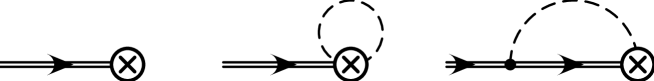
Figure 1: The three effective diagrams contributing to the width. A double line is a Vector Meson, a dashed line a pseudoscalar meson and the circled cross a vertex from ${\cal L}_{1,2,3}$.

To determine inside the effective theory the $F_{W}$ constants of Eq. (23) and (24) one has to compute the diagrams depicted in Fig. 1 and in addition the contribution coming from the Vector Meson wave function renormalization (w.f.r.). For that purpose we first define the physical vector meson basis, to be used in what follows ($T_{ext}$), fully diagonalizing the two point Green function ($G_{2}(p^{2},m_{phys}^{2}$)) at the 1–loop level, this contribution is found using the results of Ref. [3] for $G_{2}$ up to ${\cal O}(p^{4})$. This is sufficient to compute the w.f.r. as defined by

$$Z_{V}=\frac{\partial}{\partial k_{W}}G_{2}^{-1}(k_{W},m_{phys})\mid_{on-shell},$$ (25)

to order $p^{3}$, they include the electromagnetic corrections of [10]. Here $k_{W\mu}=p_{W\mu}-m_{V}v_{\mu}$ and $p_{W}^{2}=m_{W}^{2}$, $k_{W}$ is the momentum in the HMET.

The other contributions are found by direct calculation using Eq. (20) and Eq. (22). We define

$$\chi_{+}^{0}=\left.\chi_{+}\right|_{u=0}\quad\mbox{ and }\quad Q_{+}^{0}=\left.Q_{+}\right|_{u=0}\quad$$ (26)

to be the quantities $Q_{+}$ and $\chi$ with $u=0$. The extension of $Q_{+}$ needed for the charged case is defined in (A.4). The contribution of the tree diagram, the first diagram of Fig. 1, to the decay constant corresponding to $T^{a}_{ext}$ is

$$\lambda_{1}\langle T_{ext}^{a}Q_{+}^{0}\rangle+\lambda_{2}\langle T_{ext}^{a}\{\chi_{+}^{0},Q_{+}^{0}\}\rangle\,.$$ (27)

The tadpole type (second) diagram is given by:

$$\sum_{M=1,8}{\lambda_{1}\over 4F_{\pi}^{2}}\langle T_{ext}^{a}\big{[}T^{M},\big{[}T^{M\dagger},Q_{+}^{0}\big{]}\big{]}\rangle\mu_{M}\,,$$ (28)

and finally the sunrise type diagram (last diagram):

$$\sum_{M=1,8}\sum_{c=1,9}{4g\lambda_{5}\over F_{\pi}^{2}}\langle\{T_{int}^{c\dagger},T_{ext}^{a}\}T^{M}\rangle\langle T_{int}^{c}\{Q_{+}^{0},T^{M\dagger}\}\rangle K(p_{ext},\Delta m_{c},m_{M})\,,$$ (29)

where the $T_{int}$ basis was defined in [3] and the $\mu_{M}$ , $K(p_{ext},\Delta m_{c},m_{M})$ functions are defined in Eq. (B.5) of App. (B). The full result is then given by the sum of equations (27), (28) and (29) divided by the square root of the relevant $Z_{V}$. We have kept also some higher order terms required by reparametrization invariance. This corresponds to using instead of the function $K(p_{ext},\Delta m_{c},m_{M})$ the full combination $[G,\Omega]$ defined in (B).

We have checked that the non–analytical pieces of the relativistic diagram in Fig. 2 are fully recovered by the second diagram in Fig. 1 as was explicitly shown in [9] for the scalar form–factor case.

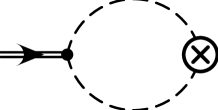
Figure 2: One of the relativistic diagram contributing to the decay constant.

6 Numerical results and conclusions

From the decay widths of Eqs. (23,24) we obtain the experimental results of the second column of Table 1. The Cabibbo-Kobayashi-Maskawa mixing angles, lifetimes, masses and branching ratios are taken from the particle data book [11].

Scenario	exp	LO	III	IV	VI
$100\lambda_{1}$ (GeV3/2)	–	6.42	6.97(36)	7.55(39)	7.74(38)
$100\lambda_{2}$ (GeV-1/2)	–	0.00	$-$0.26(50)	0.40(49)	1.21(69)
$100\lambda_{5}$ (GeV1/2)	–	0.00	3.56(75)	5.12(71)	7.24(1.43)
$F_{\rho^{0}}$ (GeV3/2)	0.0946(23)	0.0908	0.0951	0.0955	0.0937
$F_{\omega}$ (GeV3/2)	0.0287(5)	0.0303	0.0286	0.0278	0.0282
$-F_{\phi}$ (GeV3/2)	0.0565(10)	0.0428	0.0563	0.0544	0.0534
$F_{\rho^{+}}$ (GeV3/2)	0.1284(10)	input	0.1275	0.1234	0.1280
$F_{K^{*+}}$ (GeV3/2)	0.1447(45)	0.1284	0.1460	0.1571	0.1554

Table 1: The experimental Decay Constants and various good fits. The column labeled LO (lowest order) is Eq. (30) with $F_{\rho^{+}}$ as input. For an explanation of the scenarios and the values of the other constants see Table 1 in [3].

The naive prediction, using all the pure isospin states, is

$$\sqrt{2}F_{\rho^{0}}=3\sqrt{2}F_{\omega}=-3F_{\phi}=F_{\rho^{+}}=F_{K^{*+}}\,.$$ (30)

This is satisfied to about 5% for $\rho^{+},\rho^{0},\omega$, to about 13% for $\rho^{+},K^{*+}$ and about 32% for $\rho^{+},\phi$. The signs we have fixed to agree with (30).

The input parameters used are scenarios III,IV and VI from Ref. [3]. III and VI were fits to the masses only for two different values of $g$, one high and one low, fit IV also included the $\rho-\omega$ mixing in the input but otherwise as fit III. We find a reasonable fit to all the decay constants for reasonable values of $\lambda_{1,2,5}$. The higher order corrections are also reasonable, below 40%. The fit for scenario IV is worse for the following reason: Using the mixings from [3] for the $\omega$, including $p^{4}$ effects, the contributions at tree level from the $\lambda_{1}$ term essentially cancel, leaving the loop diagrams of Fig. 1 and $\lambda_{2}$ as the main contributions. This makes the predictions for the $\omega$ somewhat unstable. We also have a rather large w.f.r. factor for the $\phi$. The total size of the higher order corrections can be judged by comparing the results from Eq. (30), column LO, with those of the three scenarios.

What we have minimized in order to get the values of $\lambda_{1,2,5}$ in Table 1 is $F_{fit}=\sum_{W=1,5}\left(|F^{theo}_{W}/F^{exp}_{W}|-1\right)^{2}$. The error on the $\lambda_{i}$ corresponds to changes in $F_{fit}$ by about 0.01, i.e. at most 10% for an individual $F_{W}$, minimizing the other two $\lambda_{i}$ at the same time.

In conclusion we have calculated the corrections to the vector decay constants in heavy vector meson chiral perturbation theory and found acceptable fits to all the measured ones. We have determined 5 observables in terms of 3 parameters.

Appendix A Weak currents

In this appendix we give the main features to incorporate charged weak current effects to our formalism. The neutral weak current is not phenomenologically relevant at present. To do so one needs to extend the left current defined in Eq. (2) to:

$$l_{\mu}=eQA_{\mu}+{e\over\sqrt{2}\sin{\theta_{W}}}({\cal W}_{\mu}^{\dagger}T_{+}+{\cal W}_{\mu}T_{-})$$ (A.1)

where $\sin(\theta_{W})$ is Weinberg’s angle, ${\cal W}_{\mu}$ parametrizes the spin–1 gauge boson fields – it creates an $W^{+}$ gauge boson field and destroys an $W^{-}$ one - and we have introduced the $T$ matrices in terms of the relevant Cabibbo– Kobayashi–Maskawa factors

$$T_{+}=\left(\begin{array}[]{ccc}0&V_{ud}&V_{us}\\ 0&0&0\\ 0&0&0\end{array}\right),\qquad\qquad T_{-}=T_{+}^{\dagger}=\left(\begin{array}[]{ccc}0&0&0\\ V_{ud}&0&0\\ V_{us}&0&0\end{array}\right).$$ (A.2)

As in the QED sector, the requirement of not breaking chiral symmetry force us to split the ${\cal W}_{\mu}$ field in different components in the momenta space according to

$${\cal W}_{\mu}=e^{-im_{V}v\cdot x}\hat{\cal W}_{+\mu}+e^{im_{V}v\cdot x}\hat{\cal W}_{-\mu}^{\dagger},\qquad{\cal W}_{\mu}^{\dagger}=e^{-im_{V}v\cdot x}\hat{\cal W}_{-\mu}+e^{im_{V}v\cdot x}\hat{\cal W}_{+\mu}^{\dagger}\,.$$ (A.3)

The inclusion of the charged currents is now achieved by replacing

$$eQ_{+}\hat{A}_{\mu}\qquad\mbox{ by }\qquad eQ_{+}\hat{A}_{\mu}+{e\over\sqrt{2}\sin\theta_{W}}\,u(T_{+}\hat{\cal W}_{-\mu}^{\dagger}+T_{-}\hat{\cal W}_{+\mu})u^{\dagger}$$ (A.4)

in lagrangians Eq. (20), Eq. (21) and Eq. (22). Where now $P$ violation is allowed.

Appendix B Vector Decay Constant Contributions

In this appendix we show the formulae for the contribution coming from the effective diagrams of Fig. 1. Where we take the approximation of non–diagonal fields inside $T_{ext}$ and $T_{int}$, i.e. we use the pure isospin 1 state for $\rho^{0}$, pure isospin 0 for $\omega$ and $\phi$ and the $\phi$ as the pure strange vector state, i.e. we neglect here $\rho^{0}-\omega-\phi$ mixing.

For the tree level contribution we find

$$F_{\rho^{0}} = \sqrt{2}\lambda_{1}+{8\sqrt{2}\over 3}B_{0}\lambda_{2}(m_{d}+2m_{u})$$

$$F_{\omega} = {\sqrt{2}\over 3}\lambda_{1}-{8\sqrt{2}\over 3}B_{0}\lambda_{2}(m_{d}-2m_{u})$$

$$F_{\phi} = -{2\over 3}\lambda_{1}-{16\over 3}B_{0}m_{s}\lambda_{2}$$

$$F_{\rho^{+}} = 2\lambda_{1}+8B_{0}(m_{u}+m_{d})\lambda_{2}$$

$$F_{K^{*+}} = 2\lambda_{1}+8B_{0}(m_{u}+m_{s})\lambda_{2}\,.$$ (B.1)

For the tadpole type diagrams, we find

$$F_{\rho^{0}} = {\lambda_{1}\over\sqrt{2}F_{\pi}^{2}}(\mu_{K^{+}}+2\mu_{\pi^{+}})$$

$$F_{\omega} = {\lambda_{1}\over\sqrt{2}F_{\pi}^{2}}\mu_{K^{+}}$$

$$F_{\phi} = -{\lambda_{1}\over F_{\pi}^{2}}\mu_{K^{+}}$$

$$F_{\rho^{+}} = {\lambda_{1}\over F_{\pi}^{2}}\bigg{(}{\mu_{K^{+}}\over 2}+{\mu_{K^{0}}\over 2}+\mu_{\pi^{+}}+c^{2}\mu_{\pi^{0}}+s^{2}\mu_{\eta}\bigg{)}$$

$$F_{K^{*+}} = {\lambda_{1}\over F_{\pi}^{2}}\bigg{(}\mu_{K^{+}}+{\mu_{K^{0}}\over 2}+{\mu_{\pi^{+}}\over 2}+(\sqrt{3}c+s)^{2}{\mu_{\eta}\over 4}+(c-\sqrt{3}s)^{2}{\mu_{\pi^{0}}\over 4}\bigg{)}.$$

And finally the contribution coming from the sunrise diagram

$$F_{\rho^{0}} = \Lambda\bigg{\{}\bigg{(}{cs\over 3\sqrt{6}}+{s^{2}\over\sqrt{2}}\bigg{)}[\eta,\omega]+\bigg{(}{c^{2}\over 3\sqrt{2}}+{cs\over 3\sqrt{6}}\bigg{)}[\eta,\rho^{0}]$$

$$+{1\over 3\sqrt{2}}[K^{+},K^{*+}]+{\sqrt{2}\over 3}[K^{0},K^{*0}]$$

$$+\bigg{(}{c^{2}\over\sqrt{2}}-{cs\over 3\sqrt{6}}\bigg{)}[\pi^{0},\omega]+\bigg{(}{s^{2}\over 3\sqrt{2}}-{cs\over 3\sqrt{6}}\bigg{)}[\pi^{0},\rho^{0}]\bigg{\}}$$

$$F_{\omega} = \Lambda\bigg{\{}\bigg{(}{c^{2}\over 9\sqrt{2}}+{cs\over\sqrt{6}}\bigg{)}[\eta,\omega]+\bigg{(}{cs\over\sqrt{6}}+{s^{2}\over 3\sqrt{2}}\bigg{)}[\eta,\rho^{0}]$$

$$+{1\over 3\sqrt{2}}[K^{+},K^{*+}]-{\sqrt{2}\over 3}[K^{0},K^{*0}]$$

$$+{\sqrt{2}\over 3}[\pi^{+},\rho^{+}]+\bigg{(}{s^{2}\over 9\sqrt{2}}-{cs\over\sqrt{6}}\bigg{)}[\pi^{0},\omega]+\bigg{(}{c^{2}\over 3\sqrt{2}}-{cs\over\sqrt{6}}\bigg{)}[\pi^{0},\rho^{0}]\bigg{\}}$$

$$F_{\phi} = -\frac{\Lambda}{3}\bigg{\{}{4c^{2}\over 3}[\eta,\phi]-[K^{+},K^{*+}]+2[K^{0},K^{*0}]+{4s^{2}\over 3}[\pi^{0},\phi]\bigg{\}}$$

$$F_{\rho^{+}} = \Lambda\bigg{\{}{c^{2}\over 3}[\eta,\rho^{+}]+{1\over 2}[K^{+},K^{*0}]+{1\over 2}[K^{0},K^{*+}]+[\pi^{+},\omega]+{s^{2}\over 3}[\pi^{0},\rho^{+}]\bigg{\}}$$

$$F_{K^{*+}} = {\Lambda\over 2}\bigg{\{}{1\over 2}\bigg{(}{c\over\sqrt{3}}-s\bigg{)}^{2}[\eta,K^{*+}]+{1\over 2}[K^{+},\omega]+[K^{+},\phi]+{1\over 2}[K^{+},\rho_{0}]$$ (B.3)

$$+[K^{0},\rho^{+}]+[\pi^{+},K^{*0}]+{1\over 2}\bigg{(}c+{s\over\sqrt{3}}\bigg{)}^{2}[\pi^{0},K^{*+}]\bigg{\}}$$

with

$$\Lambda={16g\lambda_{5}\over F_{\pi}^{2}},\quad\cos\theta=c\quad and\quad\sin\theta=s.$$ (B.4)

In addition to Eq. (B), Eq. (B) and Eq. (B) one has the w.f.r. terms.

We have defined the following integrals

$$i(Kg_{\mu\nu}+Lv_{\mu}v_{\nu})=\int\frac{d^{d}q}{(2\pi)^{d}}\frac{q_{\mu}q_{\nu}}{v\cdot q-\omega+i\eta}\frac{1}{q^{2}-m^{2}+i\eta}$$ (B.5)

$$i\mu_{m}=\int\frac{d^{d}q}{(2\pi)^{d}}\frac{1}{q^{2}-m^{2}}=\frac{im^{2}}{16\pi^{2}}\left[\lambda-\log\left(\frac{m^{2}}{\mu^{2}}\right)\right]\,,$$

with $\lambda=1/\epsilon-\gamma+\log(4\pi)+1$ and $d=4-2\epsilon$, and

$$[G,\Omega]=\left(1+{p\cdot v\over m_{V}}-{m_{G}^{2}\over 2m_{V}}{\partial\over\partial m_{\Omega}}\right)K(m_{G},m_{\Omega}-m_{V}-{p\cdot v})\\$$

Here $\eta$ and $\pi_{0}$ stand for the physical pseudoscalar fields.

References

[1] E. Jenkins, A. Manohar and M. Wise, Phys. Rev. Lett. 75
(1995) 2272.
[2] E. Jenkins and A. Manohar, Phys. Lett. B255 (1991) 558
[3] J. Bijnens, P. Gosdzinsky, P. Talavera Nucl. Phys. B501
(1997) 495.
[4] H. Davoudiasl and M. Wise, Phys. Rev. D53 (1996) 2523.
[5] C–K. Chow and S–J. Rey, hep-ph/9708432.
[6] G. Ecker, Prog.Part.Nucl.Phys.35 (1995) 1;
J Gasser, Aspects of Chiral Dynamics, hep-ph/9711503
[7] M. Luke and A. V. Manohar, Phys. Lett. B286 (1992) 348.
[8] H. Georgi, Phys. Lett. B240, (1990) 447.
[9] J. Bijnens, P. Gosdzinsky, P. Talavera, hep-ph/9708232,
LU TP 97/16 and NORDITA-97/50 N/P.
[10] J. Bijnens and P. Gosdzinsky, Phys. Lett. B388 (1996) 203
[11] Review of Particle Physics, R.M. Barnett et al.,
Phys. Rev. D54 (1996) 1