MIT-CTP-2708

Supersymmetric Partners of Oblique Corrections

Emanuel Katz, Lisa Randall and Shufang Su
Center for Theoretical Physics
Laboratory for Nuclear Science and Department of Physics
Massachusetts Institute of Technology
Cambridge, MA 02139, USA

Abstract

We discuss the violation of the equality of the gauge coupling and gaugino coupling in the presence of soft supersymmetry breaking. Although this is a hard supersymmetry breaking effect, there are finite contributions to this difference which can be determined as a function of the soft supersymmetry breaking masses. The largest sources of this difference are the “super-oblique” corrections, which can be enhanced by a multiplicity factor and a logarithm of the soft supersymmetry breaking mass. This is to be contrasted to standard oblique corrections to the electroweak sector which decouple for large supersymmetry breaking. We show that these parameters can be relatively large, particularly in models of supersymmetry breaking motivated by solving the supersymmetric flavor problem. We also perform a detailed study of the non-oblique corrections for the example of squark decay. We find that they can be significant, and should be accounted for in the theoretical prediction.

1 Introduction

Supersymmetry has yet to be discovered. If/When it is, the information about the underlying theory will be limited but powerful. For example, the spectrum of superpartners might tell us about the mechanism of communication of supersymmetry breaking. It is conceivable that there is very large supersymmetry breaking within multiplets and that there are many as-yet undetected multiplets carrying standard model gauge charge. Although the heavy superparticles will elude direct detection, there can be large virtual effects which could be detectable through the difference in the gauge and gaugino coupling.

In this paper, we will discuss a new category of precision measurements which one might use to probe supersymmetric theories. As we will discuss in detail in Sec. 2, these measurements have much in common with the well-studied “oblique” corrections which characterize corrections to the standard model. In supersymmetry, the gauge coupling $g$ is equal to the gaugino Yukawa coupling $\tilde{g}$ when supersymmetry is exact. However, when supersymmetry is broken, components of the supermultiplet (for example, q and q̃) no longer have the same masses, which leads to different contributions to gauge and gaugino propagators. This is the supersymmetric analog of the “oblique” corrections and gives rise to finite differences between $g$ and $\tilde{g}$. The experiments will certainly be more difficult because they require very precise measurements and good measurements of other supersymmetric parameters. However, these measurements could yield invaluable insights into the underlying physics of supersymmetry breaking.

The key to understanding the quantities we wish to consider is to distinguish hard and soft supersymmetry breaking parameters. Supersymmetry can only be broken softly if it is to serve as a solution to the hierarchy problem. The focus of most research on supersymmetric phenomenology is on the soft supersymmetry breaking parameters, and in particular the superpartner masses. Hard supersymmetry breaking, on the other hand, is “forbidden”. However, this is not true, even in the softly broken supersymmetric theory! The only constraint is that the coefficients of hard supersymmetry breaking operators are finite. There are no available counterterms in the supersymmetric Lagrangian. Nonetheless, finite corrections are permissible and present. This is precisely analogous to the precision electroweak parameters $S$, $T$, and $U$ which are parameters of the effective theory which can be calculated as a function of the underlying heavy masses. In fact, our focus here is on new parameters which reflect hard supersymmetry breaking in the form of oblique corrections in the gauge sector as well. As with the precision electroweak parameters, these parameters will serve as a test of the supersymmetric model, and give insights into non-standard physics. While the standard oblique corrections were sensitive to large violations of custodial SU(2) symmetry, the super-oblique corrections are sensitive to large splittings within a supersymmetric multiplet.

The largest effects will occur if some superpartners have multi-TeV masses, though there are potentially measurable effects even with smaller mass splittings. Examples of models with large mass splittings are given in [1, 2, 3, 4] in which the partners of the first two generations are heavy, suppressing potential flavor changing neutral current (FCNC) problems. The squark masses could also be heavier than the slepton masses because of the larger contribution from the running of the masses due to the SU(3) strong coupling constant, or because of a larger tree-level mass in a gauge-mediated model. In Sec. 4 we present three different models which give different predictions of the super-oblique corrections motivated by these considerations and compare the effects.

Oblique corrections are also important because they are process independent, and therefore can be constrained by different experiments. Non-oblique corrections on the other hand depend on the particular process under consideration. Furthermore, virtual heavy states decouple and will not give large effects. Finally, there is no multiplicity factor (if there are many multiplets with large splittings). However, it is possible that non-oblique supersymmetric loop corrections could be important when extracting the oblique parameters. This is because of the enhancement by a group theory factor (from diagrams with internal gauge bosons and gauginos). Since the dominance of the oblique corrections requires that these effects are small, we have also calculated non-oblique corrections. These include vertex, wave function renormalizations, and gluon emission. A detailed check on our calculation is the cancellation of infrared divergences, as is discussed in Appendix E. For simplicity, in this paper, we apply our calculation of non-oblique corrections only to squark decay; we find the non-oblique corrections can in fact be significant. This indicates that it will be important to also incorporate non-oblique corrections in order to extract the masses of heavy parameters dominating the oblique-corrections.

Our work is in some ways complementary to the recent papers by Cheng, Feng, and Polonsky[5] and Pierce, Nojiri, and Yamada[6] who considered in greater detail methods for extracting oblique parameters from experiments. We instead focus on the theoretical “uncertainty” arising from non-oblique corrections which could corrupt the extraction of parameters if they are large. Of course, these can ultimately all be incorporated. We also add to the consideration of experimental signatures by giving the prediction for the production of $b\tilde{b}\tilde{g}$ and $t\tilde{t}\tilde{g}$ (assuming it is kinematically accessible) which could prove to be a promising method of extracting SU(3) gaugino Yukawa coupling if the supersymmetric partners are light.

We begin in Sec. 2 discussing the analogy between the super-oblique and oblique corrections and the non-decoupling effect of heavy superparticles. In Sec. 3, we present different examples of models that contain heavy superpartners. We give the results for super-oblique correction for these models in Sec. 4. In Sec. 5, we consider additional gauge representations and their contribution to the super-oblique corrections. In Sec. 6, we discuss possible ways to measure the super-oblique parameters and give the results for the $b\tilde{b}\tilde{g}$ and $t\tilde{t}\tilde{g}$ production cross sections. In Sec. 7, we investigate the non-oblique corrections and show that they could be quite significant compared to the oblique corrections. In Sec. 8, we conclude. We have several appendices with details of our calculations. Appendix A contains the $O(\alpha)$ corrections to vertices and self-energies for arbitrary parameters. Appendix B gives the super-oblique corrections. Appendix C gives the results of gluon emission, which will be necessary to cancel infrared divergences. In Appendix D, we consider the results in the limit of exact supersymmetry. Appendix E shows that the results of Appendices A and C combine to give infrared finite results. The final appendix gives the results for super-oblique corrections from a messenger sector.

2 Oblique and Super-Oblique

It is useful first to review standard oblique corrections. Precision electroweak corrections were important in that they tested consistency of the standard model and gave insight into the high-energy world. The oblique corrections are the corrections to the gauge boson propagator. The parameters which characterize the most important effects can be obtained by retaining the leading pieces in a derivative expansion, accounting for gauge invariance. The six “parameters” are $\Pi^{\prime}_{\gamma\gamma}$, $\Pi^{\prime}_{\gamma Z}$, $\Pi_{WW}$, $\Pi^{\prime}_{WW}$, $\Pi_{ZZ}$, $\Pi^{\prime}_{ZZ}$. We chose to work in the basis of tree-level mass eigenstates and retained only the nondecoupling pieces of the propagator, those of dimension four or less. It is useful to absorb three of the parameters into $g$, $g^{\prime}$, $v$, which leaves three new finite parameters which are forbidden by gauge invariance but are permitted once it is spontaneously broken. In Ref. [7], these three parameters were identified as as $\delta Z_{ZZ}$, $\delta Z_{\gamma Z}$, $\delta m_{ZZ}$. In the more widely utilized Peskin-Takeuchi naming convention, they were absorbed into parameters [8, 9] $S$, $T$, $U$, while a third popular convention from a paper of Altarelli and Barbieri [10] absorbed them in the three parameters $\epsilon_{1}$, $\epsilon_{2}$, $\epsilon_{3}$. The importance of these parameters is that even heavy states do not decouple. For example, one can compute the contributions of a heavy doublet to the standard $S$ parameter,

$$\Delta S={1\over 6\pi}\left[1-Y\log({m_{\rm N}^{2}\over m_{\rm E}^{2}})\right].$$ (2.1)

Of course, the many new particles present in a supersymmetric theory can contribute to the standard oblique corrections. In general, these effects are small because heavy superpartners decouple. However, there is a potentially more interesting class of “oblique” corrections for supersymmetric theories. Supersymmetry guarantees equality of the gauge and gaugino Yukawa couplings. When supersymmetry is broken, these are no longer guaranteed to be equal at low energy.

We consider the relative difference of the gauge and gaugino Yukawa couplings, which is sensitive to supersymmetry breaking. Due to supersymmetry, this difference is UV-finite and hence independent of the renormalization scale $\mu$. This difference could be measured by comparing the Yukawa coupling $\tilde{g}$, extracted from some physical process at energy scale $q^{2}$, to the gauge coupling $g$ at that same energy. Because $\alpha$ is reasonably small, and logarithms are not large, we choose to work to leading order in $\alpha$, rather than taking an effective theory approach and performing a full leading log calculation. This is useful since the finite pieces can be competitive with the logarithmically enhanced terms, while higher order terms are negligible. Note also that these parameters are $\mu$-independent and well defined, so one can calculate both logarithmically enhanced and nonlogarithmically enhanced contributions.

We define the gauge coupling $g(q^{2})$, and the gaugino Yukawa coupling $\tilde{g}(q^{2})$, as the couplings containing all the “super-oblique” corrections; in other words, as the couplings containing contributions to the gauge (or gaugino) propagator from all possible squarks and quarks running in the loops. We note that our definition of $g(q^{2})$ (which is process independent) differs from the convention of Ref. [11], who used an effective theory language and therefore did not include in their definition oblique contributions from light fermion loops. Our two conventions differ by these finite contributions, which are generally smaller than the logarithmic contribution but not by a substantial amount. Since one can readily calculate these additional loops, which the full order $\alpha$ calculation would require in any case, we choose to include these pieces also in our definition of oblique corrections.

Hence, in our case the difference between the couplings will receive contributions from all “super-oblique” diagrams (including the light fermion loops). These consist of the quark and squark contributions to the the gauge propagator (Fig. 6 (3) and (4)), and the gaugino propagator (Fig. 3 (2)). For general choices of superpartner masses, the difference at one loop takes the form of a function

$$\frac{g(q^{2})-\tilde{g}(q^{2})}{g(q^{2})}=\frac{\alpha}{4\pi}F_{\rm ob}\left(\frac{m_{q_{\rm i}}^{2}}{q^{2}},\frac{m_{\tilde{q_{\rm i}}}^{2}}{q^{2}},\frac{m_{\tilde{g}}^{2}}{q^{2}}\right)=\frac{\alpha}{4\pi}\frac{F_{g3}+F_{g4}-F_{\tilde{g}2}}{2},$$ (2.2)

which depends on the ratios of the various masses with the scale $q^{2}$ ($F_{g3}$, $F_{g4}$, $F_{\tilde{g}2}$ are explicitly given in Appendix A as integrals over Feynman parameters). For example, in the case of the SU(3) gauge and gaugino Yukawa couplings, the contribution of a single heavy doublet superfield to this difference at $q^{2}\sim m_{\tilde{g}}^{2}$ is

$${g_{3}-\tilde{g}_{3}\over g_{3}}={\alpha_{3}\over 24\pi}\left({\rm Log}\left({m_{\tilde{g}}\over m_{\tilde{q}}}\right)^{2}-{11\over 12}\right).$$ (2.3)

This formula is only true in the limit ${m_{q}}^{2}\ll{q}^{2}$ and $q^{2}\ll{m_{\tilde{q}}}^{2}$. A detailed derivation of this formula is given in Appendix B. Also notice that because physical quarks are generally lighter than the gauginos, the logarithm is cut off at the gaugino mass. Therefore, the logarithm is only large if there is a sizable splitting between the squark or slepton and gaugino masses.

Although the oblique corrections first arise at one loop (and there is an additional 1/6 suppression compared to the usual $\alpha/(4\pi)$), there are factors which can make it large. First of all, we see that there is a logarithm; if there is a large mass splitting, there will be a corresponding enhancement. Second, there is a multiplicity factor; “every” particle with gauge charge contributes. The logarithm here differs from standard oblique corrections in that decoupling works differently. Heavy scalar superpartners contribute more rather than less.

If we call the soft scalar mass $m_{0}$ and the coefficient of the trilinear scalar coupling $A$, for the standard oblique corrections (e.g. the $S$ parameter), it is easy to see that

$$\Delta S\propto{m_{\rm LR}^{2}\over m^{2}}\sim{(\lambda_{q}Am_{q})^{2}\over m_{0}^{2}},$$ (2.4)

which decouples for large $m_{0}$.

In the case of the super-oblique corrections which we discuss, one finds

$$\delta g(m_{q})\propto{\rm Log}{m_{\tilde{q}}^{2}\over m_{q}^{2}},$$ (2.5)

(where we now assume the quark mass is bigger than the gaugino’s and take $q^{2}\sim{m_{q}}^{2}$) which clearly does not decouple, and is in fact logarithmically enhanced. This logarithm can however be readily understood [12]. If we assume a chiral multiplet in which the scalar partner is heavy, there is an energy regime between the fermion (or gaugino) mass and the heavy scalar mass in which the gauge and gaugino coupling run differently. In fact one can also determine that when the scalar is the heavy partner, the gauge coupling at low energy will be reduced relative to the gaugino couplings due to the sign of the fermion contribution to the $\beta$ function for the gauge coupling.

Decoupling does occur however for super-oblique corrections when $m_{q}\sim m_{\tilde{q}}$

$$\delta g\propto{(m_{\tilde{q}}^{2}-m_{q}^{2})\over m_{q}^{2}}.$$ (2.6)

Notice here that we have assumed the squark and quark to be nearly degenerate and heavier than the gaugino. Therefore what is relevant to super-oblique corrections are standard model gauge charge multiplets with large supersymmetry breaking splitting in the masses. If these mass splittings are not very large, the constant term $11/12$ in Eq. 2.3 can be somewhat significant. For instance, if $m_{\tilde{q}}=5m_{\tilde{g}}$ the constant term is a $30\%$ correction to the logarithm.

We conclude that heavy scalar partners can lead to interesting deviations from the exact supersymmetric prediction $g=\tilde{g}$.

3 Large Effects and FCNC

It is reasonable to ask whether there is any reason to believe that there are large mass splittings. The answer might be yes, given the current ideas for resolving the FCNC problems in supersymmetric theories. The apparent degeneracy of squarks or alignment with quarks is still not understood. There are two types of scenarios which offer the possibility of large mass splittings among the superpartners. It could be that squarks (and gluinos) are heavier because of the larger SU(3) coupling. Alternatively, a suggested resolution of the FCNC problem involves heavy first two generations [1, 13, 2, 3].

An example of a class of models in which the colored states are heavy is the gauge-mediated models which have been suggested as a resolution of the FCNC problem. It could also be that colored scalars get enhanced masses from renormalization group running. Of course, either of these scenarios would probably make both the squarks and gluino heavy. A very heavy gluino would not be subject to the experimental tests we are discussing, although there could still be measurable oblique corrections for the SU(2) and U(1) sectors. Just to test how big the effects can reasonably be expected to be in a model in which the differences between the gauge coupling and gaugino Yukawa coupling can all be measured, we took a toy model with heavy squarks and a relatively light gluino. Although not motivated by any particular model, it serves to illustrate the potential size of the oblique corrections.

There are several groups who investigated the possibility of heavy first two generations. An example of such a model is [2], where an anomalous U(1) symmetry which served as a mediator of supersymmetry breaking was introduced. If only the first two generations are charged, their mass can be of order $4\pi$ bigger than the lighter third generation states. The gauginos are also among the light states. In Ref. [3], the heaviness of the first two generations is achieved through the constraints of naturalness with some restrictions on fine tuning. All the superparticles can be divided into two groups. The first, called “the brothers of the Higgs”, contains superpartners whose masses will strongly influence the mass running of the Higgs and thus are strong constrained by naturalness. The second, called “the cousins of the Higgs”, consists of superparticels which are less constrained and hence can be heavy. The first two generation squarks are in the latter group and their mass can be in the range of 900 GeV$-$5 TeV. Related ideas are incorporated into the “More Minimal Supersymmetric Standard Model” (also called effective supersymmetry)[1], in which one attempts to allow the maximal masses consistent with naturalness bounds. In this model, a new gauge group $G$ is introduced, which enlarges the accidental symmetry group and thus forbids the renormalizable $B$ and $L$ violating interactions. It also introduces a new mass scale $\tilde{M}\sim 5-20$ TeV which sets the mass scale of the first two generations. This model permits the first two generations of squarks to be heavier which goes a considerable way towards solving flavor changing problems. In addition, the requirement of naturalness implies that some squarks ($\tilde{t}_{\rm L},\tilde{b}_{\rm L}$) and most gauginos must have a mass below $\sim 1$ TeV. One can then imagine $\tilde{m}_{1,2}\sim 20$ TeV, $\tilde{m}_{3}\sim 100$ GeV $-$ 1 TeV.

4 Parameters and Numbers

One can now ask for the magnitude of the finite difference between the gauge and Yukawa couplings for the kinds of models described above. There are three measurable quantities associated with $g_{3}$, $g_{2}$, $g_{1}$, which are the coupling constants of the gauge groups SU(3), SU(2) and U(1) respectively. These fit in well with a modified Peskin-Takeuchi naming convention $v=(g_{3}-\tilde{g}_{3})/g_{3}$, $w=(g_{2}-\tilde{g}_{2})/g_{2}$, $y=(g_{1}-\tilde{g}_{1})/g_{1}$.

We now present the magnitude of each of these quantities for the types of models described in Sec. 3 in which there are mass splittings. We make simple assumptions below to get an idea of the magnitude of the effects. In the following we will use the value of the various couplings at $M_{Z}$ to estimate the effects, and we take $q^{2}\sim{m}_{\rm gaugino}^{2}$.

We define three different models:

Model 1

Only the squarks are heavy. We take $R_{\tilde{q}}^{\tilde{W}}\equiv{m}_{\tilde{W}}/m_{\tilde{q}}=0.05$, and since this is a gauge mediated model $m_{\tilde{g}}:m_{\tilde{W}}=\alpha_{3}:\alpha_{2}\approx 7:2$,where $\alpha_{3}=0.12$, $\alpha_{e}=1/128$, $\sin^{2}\theta_{W}=0.23$. Thus, $R_{\tilde{q}}^{\tilde{g}}\equiv{m}_{\tilde{g}}/m_{\tilde{q}}=0.18$. In Table 1, we present the numerical results for Model 1.

$\hskip 65.04256ptv\hskip 36.135pt$	$3.82\%\log{R}_{\tilde{q}}^{\tilde{g}}-1.8\%$	-8.4%
$\hskip 65.04256ptw\hskip 36.135pt$	$0.81\%\log{R}_{\tilde{q}}^{\tilde{W}}-0.37\%$	-2.8%
$\hskip 65.04256pty\hskip 36.135pt$	$0.30\%\log{R}_{\tilde{q}}^{\tilde{W}}-0.14\%$	-1.0%

Table 1: Super-oblique corrections for Model 1.

Here we have ignored the additional finite contribution from the sleptons. If, for example, $m_{\tilde{l}}=m_{\tilde{W}}$, one calculates the finite contribution $\alpha_{2}/24\pi(11/2-\sqrt{3}\pi/2)$ instead of $\alpha_{2}/24\pi(-11/12)$ in Eq. 2.3 (where we consider SU(2) case, and similarly for U(1) case).

Model 2

A More Minimal Spectrum, in which the masses of $b_{\rm R}$, $u$, $d$, $s$, $c$, $e$, $\mu$ are $m_{\rm H}=20$ TeV, whereas the masses of $b_{\rm L}$, $t$, $\tau$ are $m_{\rm L}=$1 TeV, while $m_{\tilde{W}}=100{\rm GeV}$, and $m_{\tilde{g}}=350{\rm GeV}$. In this model, $R_{\rm L}^{\tilde{g}}\equiv{m_{\tilde{g}}}/{m}_{\rm L}=0.35$, $R_{\rm H}^{\tilde{g}}\equiv{m_{\tilde{g}}}/{m}_{\rm H}=0.018$, $R_{\rm L}^{\tilde{W}}\equiv{m}_{\tilde{W}}/{m}_{\rm L}=0.1$ and $R_{\rm H}^{\tilde{W}}\equiv{m}_{\tilde{W}}/{m}_{\rm H}=0.005$. In Table 2, we present the numerical results for Model 2.

$\hskip 43.36243ptv\hskip 14.45377pt$	$0.95\%\log{R}_{\rm L}^{\tilde{g}}+2.86\%\log{R}_{\rm H}^{\tilde{g}}-1.8\%$	-14.3%
$\hskip 43.36243ptw\hskip 14.45377pt$	$0.36\%\log{R}_{\rm L}^{\tilde{W}}+0.72\%\log{R}_{\rm H}^{\tilde{W}}-0.5\%$	-5.1%
$\hskip 43.36243pty\hskip 14.45377pt$	$0.16\%\log{R}_{\rm L}^{\tilde{W}}+0.38\%\log{R}_{\rm H}^{\tilde{W}}-0.25\%$	-2.6%

Table 2: Super-oblique corrections for Model 2.

Model 3

A modified more minimal model similar to Model 2, in which the sleptons have mass $m_{\rm L}=$1 TeV. In Table 3, we present the numerical results for Model 3.

$\hskip 43.36243ptv\hskip 14.45377pt$	$0.95\%\log{R}_{\rm L}^{\tilde{g}}+2.86\%\log{R}_{\rm H}^{\tilde{g}}-1.8\%$	-14.3 %
$\hskip 43.36243ptw\hskip 14.45377pt$	$0.54\%\log{R}_{\rm L}^{\tilde{W}}+0.54\%\log{R}_{\rm H}^{\tilde{W}}-0.5\%$	-4.6%
$\hskip 43.36243pty\hskip 14.45377pt$	$0.32\%\log{R}_{\rm L}^{\tilde{W}}+0.22\%\log{R}_{\rm H}^{\tilde{W}}-0.25\%$	-2.2%

Table 3: Super-oblique corrections for Model 3.

We can see that $v$ is the same for Models 2 and 3 since changing the slepton mass would not affect the SU(3) coupling constant, which only gets contributions from q, q̃ and g̃. $v$ is much larger than $w$ and $y$ since the corresponding coupling is much larger. We write the super-oblique corrections in terms of the ratio of the mass splittings in Tables 1, 2, 3, where it is evident that the finite piece 11/12 does give a sizable contribution if the logarithm is not much larger than 1. The results we get for Model 1 are consistent with the results for the “heavy QCD models” in Ref. [14] when the gluino is light. Our model 2 is close to the “2-1 models” [14] except that we put $b_{\rm R}$ in the heavy sector. When we let $b_{\rm R}$ also be light, the coefficient before $\log{R}^{\tilde{W}}_{H}$ in Model 2 also fits well with the results given in Ref. [14]. However, in our case, we also calculate the contribution from the finite piece 11/12 and the light squarks, whose masses are still large enough (compared to the gauginos) to give noticeable contribution.

5 More Non-Standard Physics

In this section, we consider the role of the super-oblique correction measurements not only as a test of the parameters of the minimal extension of the standard model but also as a potential probe of other new physics. We have already stressed the fact that heavy squarks can be large. This is especially important as it is precisely when the squarks become kinematically inaccessible that their virtual effects become largest. If one does not find the squarks, or if they are at the edge of the kinematically accessible regime, one would like to be able to confirm their existence and attempt some estimate of their mass through their virtual effects.

However, it might be that the squarks are relatively light, and one still measures large deviations from the supersymmetric relations. Provided they are not too large, one might ask how this could be consistent with supersymmetry. In fact, this is probably the most exciting possibility. It would indicate the existence of nonstandard fields which participate in supersymmetry breaking and therefore have a large mass splitting relative to the mass of the fermions or scalars and which carry standard model gauge charge. An obvious candidate in terms of existing models is a messenger sector, although possibilities extend beyond this. As an example, suppose the messenger sector consisted of a large vectorlike representation under SU(5). One should note that for the “standard” messenger scenario, with a singlet coupled to messengers through a Yukawa term, the masses of the scalars are $\sqrt{\lambda^{2}S^{2}\pm\lambda F_{\rm S}}$ whereas the fermion mass is $\lambda S$. In this case, $q^{2}$ (the external four-momentum squared for $g$ and g̃) is taken to be smaller than the fermion mass. We take the limit $q^{2}\ll{m}_{\rm fermion}^{2}$, $q^{2}\ll{m}_{\rm scalar}^{2}$ to calculate the super-oblique corrections. Let $m_{\rm scalar}^{2}/m_{\rm fermion}^{2}=1\pm{x}$. The effects are unfortunately small unless $x$ is very close to 1 (see Appendix F). Without an enormous multiplicity factor, a nontrivial mass splitting is needed to get a sizable contribution.

6 Measurements of Oblique Parameters

It is clear that there can be fairly sizable effects. It is therefore extremely interesting to ask the question whether the parameters can be measured. The numbers presented above serve as benchmarks for interesting measurements, although a measurement at any level of accuracy will constrain our confidence in supersymmetry or equivalently constrain extensions of the minimal scenario.

Several groups have begun to investigate this question. Initially this was pursued as a test of supersymmetry at tree level [11] and it was later studied in order to extract squark masses if they are heavy [12, 5]. More recently, several groups, [15, 11, 14, 6] have studied super-oblique corrections. We summarize some suggestions for measurements. We also present new results for the $b\tilde{b}\tilde{g}$ and $t\tilde{t}\tilde{g}$ productions.

One measurement which has been suggested of the U(1) coupling is in a paper by Nojiri, Fujii, and Tsukamoto [12] where they studied $\sigma(e^{+}e^{-}\to\tilde{e}_{\rm R}^{+}\tilde{e}_{\rm R}^{-})$. This process proceeds through $s$-channel gauge exchange and $t$-channel neutralino exchange. One can measure $\tilde{g}_{1}$ and $M_{1}$ by measuring the angular distribution of the differential cross section ${d\sigma(e^{+}e^{-}\to\tilde{e}_{\rm R}^{+}\tilde{e}_{\rm R}^{-})}/{d\cos\theta}$. It has also been suggested by Cheng, Feng, and Polonsky [5] to look at the $e^{-}e^{-}$ scattering cross section through $t$-channel neutralino exchange when running the collider in the appropriate mode. This can lead to even greater precision since some of the troublesome backgrounds are absent and the ability to highly polarize the beams increases the $\tilde{e}_{R}\tilde{e}_{R}$ cross section further [11, 14]. It should be borne in mind that although the U(1) coupling might be the most accurately measured, the magnitude of $y$ is the smallest of the three precision measurements. It is therefore worthwhile to investigate the possibility of measuring $w$ and $v$ as well.

Several ways of measuring $w$ have been suggested; the most appropriate will depend on the region of supersymmetry parameter space which is realized [11, 5]. We summarize some of the suggestions of Ref. [5]. If the charginos are kinematically accessible, their production cross section can be used to measure $w$, for example if they are pair produced with a contribution from sneutrino exchange. Neutralino production (and decay if more than one mode is sizable) can also be used to test $w$ (and $y$). It might also be possible to test the gaugino coupling through the chargino mass dependence on the $H\tilde{H}\tilde{W}$ vertex, though this will help only away from the region where charginos are nearly pure gaugino. It should be noted that a good measurement of $m_{\tilde{\nu}}$ will be important when constraining $w$ to high precision by some of these methods. Another possible way to study $w$ is through the branching fraction of charginos if there are appropriate modes which are kinematically accessible. Finally, selectron and sneutrino production could provide important probes.

Finally we consider the measurement of $v$, which requires measuring the SU(3) Yukawa coupling. It is very likely that the best test will be at a hadron collider, where gluino and squark can be produced abundantly. In the case that squark decay is observed, the branching ratios into gluinos and winos can serve as probes of the super-oblique corrections. Notice that the gluino production section goes primarily through the gluon coupling, and therefore does not serve as a test at all. The branching fraction tests are also possible at an $e^{+}e^{-}$ collider if squarks are sufficiently light.

At an $e^{+}e^{-}$ collider, it might be possible to test the 2-1 type models if $\tilde{t}$, $\tilde{g}$ are sufficiently light or if $\tilde{b}$, $\tilde{g}$ are sufficiently light. We consider the the cross section for $t\tilde{t}\tilde{g}$ and $b\tilde{b}\tilde{g}$ production to get an estimate of the possible sensitivity to $v$. For $b$ quark and squark production one predicts a few hundred events according to the gluino and squark mass (below a few hundred GeV) and roughly the same for the top quark. In Fig. 8 and Fig. 9 we present the numbers of events produced per year at an $e^{+}e^{-}$ collider at $E_{\rm cm}=1000$ GeV and luminosity $L=5\times 10^{33}{\rm cm}^{-2}{\rm s}^{-1}$. The number of events decreases with the increase of ${m_{\tilde{q}}}$ and ${m_{\tilde{g}}}$ due to the decrease in phase space. The number of $b$ events is slightly less than $t$ events, though their phase space is larger. This is because of the different couplings of the $b$ and $t$ to $Z$ and $\gamma$. When ${m_{\tilde{q}}}>{m_{\tilde{g}}}$, it is possible that the intermediate squark state is on shell, which gives a peak in the production rate which we have not shown. This is more significant to $b\tilde{b}\tilde{g}$ production since $m_{b}\sim{4}$ GeV, so there is a larger range of parameters for which the intermediate $\tilde{b}$ is on shell. In this case one is in fact measuring the squark decay branching ratio into gluino, which can also determine the gaugino Yukawa coupling. By measuring the branching ratio for the decay of the q̃  into $\tilde{q}\rightarrow{q}\tilde{g}$, $\tilde{q}\rightarrow{q^{\prime}}\tilde{\chi}^{\pm}$ and $\tilde{q}\rightarrow{q}\tilde{\chi}^{0}$, one can hope to extract the coupling, if the other parameters (masses) can be independently determined [14]. The number of events we present here is the event production, not corrected for cuts necessary to remove background events. Nonetheless for sufficiently light gaugino and third generation squarks, it seems likely that a measurement of the gaugino coupling at at least the 15% level should be possible.

7 Non-oblique Contributions

When extracting the q̃qg̃ coupling from a physical process, such as squark decay branching fractions, it is important to consider finite contributions from non-oblique diagrams. Although one usually ignores such terms, they could be significant because of the $C_{2}(G)$ factor ($C_{2}(G)=N$ for SU(N)). For instance, in the non-abelian gluon and gluino loop diagrams (Fig. 2 (4)), even though there are no large logarithms, the $C_{2}(G)$ acts as a multiplicity factor, enhancing their effect. Hence, it is useful to check the relative size of the non-oblique corrections.

It is important to bear in mind that the $\mu$ dependence in the oblique parameters cancel; everything is finite. We will sometimes refer to finite pieces; by this we mean the nonlogarithmically enhanced contribution (that is, the finite pieces in an effective theory approach). The finiteness is important in that it means that the answer at one-loop is renormalization scheme independent. The dependence on momentum is through the dependence on the physical momenta which enter the loops. For any given process these are specified. For example, in the case of squark decay, the mass squared of the squark will enter. In a process with a virtual squark, the loops will be functions of $q^{2}$ and the squark mass squared; the $q^{2}$ dependence of the virtual corrections can be incorporated when one integrates over $q^{2}$. Because it is clearly simpler, we illustrate the non-oblique corrections (which are process dependent) with the specific case of squark decay. One can however apply our results to any process by which the oblique parameters will be measured.

Now let us focus on the q̃ decay process $\tilde{q}\rightarrow{q}\tilde{g}$. The relevant non-oblique diagrams include the quark and squark self energies (Fig. 4, Fig. 5), the non-abelian gluon and gluino self energies (Fig. 6 (1), (2) and Fig. 3 (1)), the $\tilde{q}q\tilde{g}$ vertex diagrams (Fig. 2), and the gluon emission diagrams (Fig. 7). Here, all the diagrams are necessary to render a gauge invariant answer free of infrared divergencies. The quark and gluino are assumed to be always on shell, while the squark could be offshell at energy $q^{2}$. We note that for completeness we have included both abelian diagrams (Fig. 2 (1), (2), Fig. 4, Fig. 5) (proportional to $C_{2}(N)$), and non-abelian diagrams (Fig. 2 (3), (4), Fig. 3 (1), Fig. 6 (1), (2)) (proportional to $C_{2}(G)$). We use the dimensional reduction regularization scheme ($\overline{DR}$), rather than dimensional regularization, to avoid obtaining a finite difference between the gauge and the Yukawa couplings in the supersymmetric limit. This finite difference occurs in dimensional regularization because of the mismatch of fermionic and bosonic degrees of freedom for dimension $d>4$.

In addition, we introduce a gluon mass, $\lambda$, to regulate infrared divergencies. Since the quark mass is usualy much smaller than that of the squark and gluino, we could have set $m_{q}$ to zero. However, we found that because $m_{q}$ effectively regulates the collinear divergences in the angular integral of the real gluon emission, keeping it non-zero made it easier to keep track of the various sources of divergences. As a result, separation of soft emission divergences, proportional to the logarithm of $\lambda$, from those of collinearity (proportional to the logarithm of $m_{q}$) was straightforward. Identifying the infrared divergence in a given vertex diagram with the corresponding divergence in the emission diagram, we were able to explicitly verify that the sum of diagrams is infrared finite (see Appendix E). The total UV-finite virtual non-oblique correction is defined to be

$$F_{\rm virtual}(q^{2},m_{q}^{2},m_{\tilde{q}}^{2},m_{\tilde{g}}^{2},\lambda^{2})=\sum_{i=1}^{4}\tilde{F}_{\rm Vi}+\frac{1}{2}\sum_{{\rm i}=1}^{2}F_{q{\rm i}}+\frac{1}{2}\sum_{{\rm i}=1}^{2}F_{\tilde{q}{\rm i}}+\frac{1}{2}F_{\tilde{g}1},$$ (7.1)

Here, the $\tilde{F}_{\rm Vi}$ are the vertex diagrams contributions, and $F_{q{\rm i}}$, $F_{\tilde{q}{\rm i}}$, $F_{\tilde{g}1}$ are the quark, squark, and gluino self-energies. All the $F$s are explicitly given in terms of integrals over Feynman parameters in Appendix A. We also define the UV-finite contribution arising from gluon emission, $F_{\rm emission}$, by

$$\Gamma_{\tilde{q}\rightarrow q\tilde{g}g}(q^{2})=\frac{\tilde{\alpha}}{4\pi}\tilde{\Gamma}_{0}(q^{2})F_{\rm emission}(q^{2},m_{q}^{2},m_{\tilde{q}}^{2},m_{\tilde{g}}^{2},\lambda^{2}).$$ (7.2)

Here, $\tilde{\Gamma}_{0}$ is the tree level decay rate for $\tilde{q}\rightarrow{q}\tilde{g}$ and its explicit formula is given in Eq. C.6. Note that in the three-body final state decay we are integrating over all of phase space, effectively including soft and hard gluon emission. This constitutes an overestimate of the emission finite contribution. However, the sign is the opposite to the overall sign of the non-oblique corrections, so this constitutes an underestimate of their size.

The total squark decay width is thus given by

$$\Gamma_{\rm total}=\tilde{\Gamma}_{0}\left(1+\frac{\tilde{\alpha}}{4\pi}(2F_{\rm virtual}+F_{\rm emission})\right).$$ (7.3)

Recall that in Eq. 2.2

$$\frac{g(q^{2})-\tilde{g}(q^{2})}{g(q^{2})}=\frac{\alpha}{4\pi}F_{\rm ob},$$ (7.4)

then

$$\tilde{\alpha}=\alpha(1-\frac{\alpha}{4\pi}2F_{\rm ob}).$$ (7.5)

Combining Eq. 7.3 and 7.5 (We use $\alpha$ in stead of $\tilde{\alpha}$ in Eq. 7.3 because the difference is high order.), the squark decay width is given in terms of $g(q^{2})$ as

$$\Gamma_{\rm total} = \Gamma_{0}\left(1+\frac{\alpha}{4\pi}(2F_{\rm virtual}+F_{\rm emission}-2F_{\rm ob})\right)$$ (7.6)

$$= \Gamma_{0}\left(1+\frac{\alpha}{4\pi}(2F_{\rm non-ob}-2F_{\rm ob})\right),$$

where $F_{\rm non-ob}$ is defined by $F_{\rm non-ob}=F_{\rm virtual}+1/2F_{\rm emission}$ and $\Gamma_{0}$ is similar to $\tilde{\Gamma}_{0}$ except that the coupling constant is $g$ instead of $\tilde{g}$.

The numerical results for SU(3) $(\alpha/4\pi)F_{\rm non-ob}$ for on shell q̃ decay is shown in Fig. 10. For a range of ${m_{\tilde{g}}}/{m_{\tilde{q}}}$ of $0.5-0.8$, which is a reasonable range for the parameters which might be accessible to an $e^{+}e^{-}$ collider, $(\alpha/4\pi)F_{\rm non-ob}$ changes from -8.5% to -1.57%. This can be a significant fraction of $v$. Furthermore, it has the same sign to $F_{\rm ob}$ contributions, thereby lessening the observed effect (Notice the relative minus sign between $F_{\rm ob}$ and $F_{\rm non-ob}$). This cancellation is more significant when ${m_{\tilde{g}}}/{m_{\tilde{q}}}$ is smaller. Recall that we are imagining a model like Model 2. For $m_{\tilde{g}}/m_{\rm L}=0.5-0.8$, with $m_{\rm L}/m_{\rm H}=1/20$, we obtain $v=-10.2\%\rightarrow-9.7\%$ (where the parameter is given at $q^{2}=m_{\rm L}^{2}$).

It might seem surprising that the non-oblique corrections are larger in magnitude for smaller ${m_{\tilde{g}}}/{m_{\tilde{q}}}$, which seems to contradict the decoupling effect of the heavy sectors. Actually this is due to some large negative total shift of the non-oblique corrections with respect to zero, while $F_{\rm non-ob}$ still goes proportional to ${m_{\tilde{g}}}/{m_{\tilde{q}}}$, especially when the ratio is small, which shows the decoupling effect of the heavy sector.

$F_{\rm non-ob}$ for SU(2) can be obtained similarly, and is -1.43% for $m_{\tilde{W}}/m_{\tilde{l}}=0.5$ and -0.24% for $m_{\tilde{W}}/m_{\tilde{l}}=0.8$ (as compared to $w=-2.6\%\rightarrow-2.4\%$). A similar calculation for only the abelian part is done in Ref. [16], which is consistent with our result except that in their Eq. (13), the constant in $F_{\rm real}$ should be 7/2 instead of 13/4 and the $F_{\tilde{g}}$ in their Eq. (19) should have the opposite sign.

We only calculated the non-oblique corrections for on-shell squark decay. For other physical processes, the non-oblique corrections can be done similarly using the same method. For example, in the process $e^{+}e^{-}\rightarrow\tilde{W}^{+}\tilde{W}^{-}$ through t-channel $\tilde{\nu}$ exchange, one would also want to include non-oblique corrections. However, there are additional radiation diagrams which in general must be incorporated.

As an additional check of our results, we have verified that in the SUSY limit ($m_{q}=m_{\tilde{q}},m_{\tilde{g}}=0$), the non-oblique UV-finite corrections to $g_{\rm i}$ and $\tilde{g}_{\rm i}$ are identical (See Appendix D).

8 Conclusions

To conclude, it is obvious that if supersymmetry is discovered, we would like to gain as many handles on the underlying supersymmetric theory as can be accessible. Super-oblique corrections provide a different perspective into the physics of supersymmetry breaking and into the consistency of the standard supersymmetric sector. As with the standard oblique corrections, they test consistency of the simplest version of the theory and provide access to nonstandard physics. They are most useful precisely when they are largest; namely there are heavy superpartners which cannot be directly observed. The particular parameters we discussed are the supersymmetric analogs of the standard-oblique parameters. The one-loop gluon and gluino propagators give contributions to the gauge and gaugino Yukawa coupling difference, which are finite. In nonstandard models, especially those addressing the supersymmetric flavor problem, it is likely that the parameters we have described could be large. We have shown that non-oblique corrections are also potentially significant, and should be incorporated in the theoretical predictions.

The super-oblique parameters will be difficult to measure, although there are many potential candidate measurements. Clearly, the better measured are the super-oblique parameters, the more constrained will be the underlying model. These parameters merit further study, both in understanding experiments and in further calculations of non-oblique effects.

Appendix A $O({\alpha})$ corrections to Vertices and Self Energies

In Fig. 1 and 2, we show the one-loop Feynman diagrams that contribute to the corresponding gqq and q̃qg̃ vertex corrections (denoted by $F_{\rm Vi}$ and ${\tilde{F}_{\rm Vi}}$). Using the $\overline{DR}$ renormalization scheme with $D=4-2\epsilon$ and regularizing the infrared divergences by an infinitesimal gluon mass $\lambda$, we get

$$F_{\rm V1}=(C_{2}(N)-1/2C_{2}(G))\left[\frac{1}{\bar{\epsilon}}+\log\mu^{2}-1-\right.$$ (A.1)

$${\int{{\rm d}x{\rm d}y{\rm d}z\,\delta(1-x-y-z)}}(2\log((x^{2}+2xy+y^{2}){m_{q}}^{2}-xyq^{2}+z\lambda^{2})+$$

$$\left.\frac{2(2-2x-2y-x^{2}-2xy-y^{2}){m_{q}}^{2}+2(-1+x+y-xy)q^{2}}{(x^{2}+2xy+y^{2}){m_{q}}^{2}-xyq^{2}+z\lambda^{2}})\right],$$

$$F_{\rm V2}=(C_{2}(N)-1/2C_{2}(G))\left[\frac{1}{\bar{\epsilon}}+\log\mu^{2}-{\int{{\rm d}x{\rm d}y{\rm d}z\,\delta(1-x-y-z)}}\right.$$ (A.2)

$$(2\log((x+y){m_{\tilde{q}}}^{2}+z{m_{\tilde{g}}}^{2}+(-x-y+x^{2}+2xy+y^{2}){m_{q}}^{2}-xyq^{2})-$$

$$\left.\frac{4(x+y)(1-x-y){m_{q}}^{2}}{(x+y){m_{\tilde{q}}}^{2}+z{m_{\tilde{g}}}^{2}+(-x-y+x^{2}+2xy+y^{2}){m_{q}}^{2}-xyq^{2}})\right],$$

$$F_{\rm V3}=C_{2}(G)\left[\frac{3}{2\bar{\epsilon}}+\frac{3}{2}\log\mu^{2}-\frac{1}{2}-{\int{{\rm d}x{\rm d}y{\rm d}z\,\delta(1-x-y-z)}}\right.$$ (A.3)

$$(3\log((-x-y+z+x^{2}+2xy+y^{2}){m_{q}}^{2}-xyq^{2}+(x+y)\lambda^{2})+$$

$$\left.\frac{3(1-2x-2y+x^{2}+2xy+y^{2}){m_{q}}^{2}+(1+x+y-xy)q^{2}}{(-x-y+z+x^{2}+2xy+y^{2}){m_{q}}^{2}-xyq^{2}+(x+y)\lambda^{2}})\right],$$

$$F_{\rm V4}=C_{2}(G)\left[\frac{1}{2\bar{\epsilon}}+\frac{1}{2}\log\mu^{2}-\frac{1}{2}-{\int{{\rm d}x{\rm d}y{\rm d}z\,\delta(1-x-y-z)}}\right.$$ (A.4)

$$(\log(z{m_{\tilde{q}}}^{2}+(x+y){m_{\tilde{g}}}^{2}-(x+y-x^{2}-2xy-y^{2}){m_{q}}^{2}-xyq^{2})-$$

$$\left.\frac{{m_{\tilde{g}}}^{2}+(1-2x-2y+x^{2}+2xy+y^{2}){m_{q}}^{2}+xyq^{2}}{z{m_{\tilde{q}}}^{2}+(x+y){m_{\tilde{g}}}^{2}-(x+y-x^{2}-2xy-y^{2}){m_{q}}^{2}-xyq^{2}})\right],$$

$$\tilde{F}_{\rm V1}=(C_{2}(N)-1/2C_{2}(G))\left[\frac{1}{\bar{\epsilon}}+\log\mu^{2}-\frac{1}{2}-{\int{{\rm d}x{\rm d}y{\rm d}z\,\delta(1-x-y-z)}}\right.$$

$$(2\log(y{m_{\tilde{q}}}^{2}-yz{m_{\tilde{g}}}^{2}+(z-xz){m_{q}}^{2}-xyq^{2}+x\lambda^{2})+$$

$$\left.\frac{(-2x-2y+xy+y^{2}){m_{\tilde{g}}}^{2}+(1+x^{2}+xy){m_{q}}^{2}+(2x-xy)q^{2}+2z{m_{\tilde{g}}}{m_{q}}}{y{m_{\tilde{q}}}^{2}-yz{m_{\tilde{g}}}^{2}+(z-xz){m_{q}}^{2}-xyq^{2}+x\lambda^{2}})\right],$$

$$\tilde{F}_{\rm V2}=(C_{2}(N)-1/2C_{2}(G)){\int{{\rm d}x{\rm d}y{\rm d}z\,\delta(1-x-y-z)}}$$ (A.6)

$$\frac{2((1-y){m_{\tilde{g}}}^{2}+(1-x){m_{q}}^{2}+(x+y){m_{\tilde{g}}}{m_{q}})}{z{m_{\tilde{q}}}^{2}+(x-y+xy+y^{2}){m_{\tilde{g}}}^{2}+(-x+y+x^{2}+xy){m_{q}}^{2}-xyq^{2}},$$

$$\tilde{F}_{\rm V3}=C_{2}(G)\left[\frac{1}{2\bar{\epsilon}}+\frac{1}{2}\log\mu^{2}-\frac{1}{4}-{\int{{\rm d}x{\rm d}y{\rm d}z\,\delta(1-x-y-z)}}\right.$$

$$(\log(x{m_{\tilde{q}}}^{2}+(-y+z+xy+y^{2}){m_{\tilde{g}}}^{2}+(-x+x^{2}+xy){m_{q}}^{2}-xyq^{2}+y\lambda^{2})+$$

$$\left.\frac{(1+xy+y^{2}){m_{\tilde{g}}}^{2}+(-2x-2y+x^{2}+xy){m_{q}}^{2}+y(2-x)q^{2}+2z{m_{\tilde{g}}}{m_{q}}}{2(x{m_{\tilde{q}}}^{2}+(-y+z+xy+y^{2}){m_{\tilde{g}}}^{2}+(-x+x^{2}+xy){m_{q}}^{2}-xyq^{2}+y\lambda^{2})})\right],$$

$$\tilde{F}_{\rm V4}=C_{2}(G)\left[\frac{2}{\bar{\epsilon}}+2\log\mu^{2}-1-{\int{{\rm d}x{\rm d}y{\rm d}z\,\delta(1-x-y-z)}}\right.$$

$$(4\log((xy+y^{2}){m_{\tilde{g}}}^{2}+(x^{2}+xy){m_{q}}^{2}-xyq^{2}+z\lambda^{2})+$$

$$\left.\frac{(1-x-2yz){m_{\tilde{g}}}^{2}+(1-y-2xz){m_{q}}^{2}-(z+2xy)q^{2}-(x+y){m_{\tilde{g}}}{m_{q}}}{(xy+y^{2}){m_{\tilde{g}}}^{2}+(x^{2}+xy){m_{q}}^{2}-xyq^{2}+z\lambda^{2}})\right].$$

Here $1/\bar{\epsilon}=1/\epsilon-\gamma_{\rm E}+\log 4\pi$, $\mu$ is the arbitrary renormalization scale, $x$, $y$, $z$ are the Feynman parameters, $q^{2}$ is the external four-momentum squared for g or q̃  and all the other external particles (q and g̃) are on shell. $C_{2}(R)$ is defined by $t^{a}(R)t^{a}(R)=C_{2}(R)\cdot{\bf 1}$, where $t^{a}(R)$ is the generator of SU(N) in the representation R with normalization ${\rm tr}[t^{a}(N)t^{b}(N)]=1/2\delta^{ab}\equiv{C}(N)\delta^{ab}$ for the fundamental representation $N$.

The one-loop corrections to the g̃ self energies are shown in Fig. 3, giving

$$F_{\tilde{g}1}=C_{2}(G)\left[-\frac{1}{\bar{\epsilon}}-\log\mu^{2}+\right.$$ (A.9)

$$2{\int{{\rm d}x{\rm d}y\,\delta(1-x-y)}}((1-x)\log(x{m_{\tilde{g}}}^{2}+(-x+x^{2})q^{2}+y\lambda^{2})+$$

$$\left.\frac{-4(-x+x^{2}){m_{\tilde{g}}}^{2}+2(1-x)(-x+x^{2})q^{2}}{x{m_{\tilde{g}}}^{2}+(-x+x^{2})q^{2}+y\lambda^{2}})\right],$$

$$F_{\tilde{g}2}=C(N)\left[-\frac{2}{\bar{\epsilon}}-2\log\mu^{2}+\right.$$ (A.10)

$$4{\int{{\rm d}x{\rm d}y\,\delta(1-x-y)}}((1-x)\log(y{m_{\tilde{q}}}^{2}+x{m_{q}}^{2}+(-x+x^{2})q^{2})+$$

$$\left.\frac{2(1-x)(-x+x^{2})q^{2}}{y{m_{\tilde{q}}}^{2}+x{m_{q}}^{2}+(-x+x^{2})q^{2}})\right].\hskip 144.54pt$$

Here again the $q^{2}$ is the external four-momentum squared of the g̃, and is the external four-momentum squared of the q, q̃ or g in the q, q̃ or g self energies below.

With the same conventions we use above, we can get the corrections to the self energies of q, q̃ and g: (the corresponding one-loop Feynman diagrams are Fig. 4, Fig. 5, and Fig. 6)

$$F_{q1}=C_{2}(N)\left[-\frac{1}{\bar{\epsilon}}-\log\mu^{2}+\right.$$ (A.11)

$$2{\int{{\rm d}x{\rm d}y\,\delta(1-x-y)}}((1-x)\log(x{m_{q}}^{2}+(-x+x^{2})q^{2}+y\lambda^{2})+$$

$$\left.\frac{2(-x+x^{2})((1-x)q^{2}-2{m_{q}}^{2})}{x{m_{q}}^{2}+(-x+x^{2})q^{2}+y\lambda^{2}})\right],\hskip 144.54pt$$

$$F_{q2}=C_{2}(N)\left[-\frac{1}{\bar{\epsilon}}-\log\mu^{2}+\right.$$ (A.12)

$$2{\int{{\rm d}x{\rm d}y\,\delta(1-x-y)}}(x\log(x{m_{\tilde{q}}}^{2}+y{m_{\tilde{g}}}^{2}+(-x+x^{2})q^{2})+$$

$$\left.\frac{2x(-x+x^{2})q^{2}}{x{m_{\tilde{q}}}^{2}+y{m_{\tilde{g}}}^{2}+(-x+x^{2})q^{2}})\right],$$

$$F_{\tilde{q}1}=C_{2}(N)\left[-\frac{2}{\bar{\epsilon}}-2\log\mu^{2}+\frac{2}{3}-\right.$$ (A.13)

$$4{\int{{\rm d}x{\rm d}y\,\delta(1-x-y)}}(3(-x+x^{2})\log(x{m_{q}}^{2}+(-x+x^{2})q^{2}+y{m_{\tilde{g}}}^{2})-$$

$$\left.\frac{x(1-x)(-x+x^{2})q^{2}}{x{m_{q}}^{2}+(-x+x^{2})q^{2}+y{m_{\tilde{g}}}^{2}})\right],$$

$$F_{\tilde{q}2}=C_{2}(N)\left[\frac{2}{\bar{\epsilon}}+2\log\mu^{2}+\frac{1}{6}-\right.$$ (A.14)

$${\int{{\rm d}x{\rm d}y\,\delta(1-x-y)}}((4-6x+3x^{2})\log(x{m_{\tilde{q}}}^{2}+(-x+x^{2})q^{2}+y\lambda^{2})+$$

$$\left.\frac{(2-x)^{2}(-x+x^{2})q^{2}}{x{m_{\tilde{q}}}^{2}+(-x+x^{2})q^{2}+y\lambda^{2}})\right],$$

$$F_{g1}=C_{2}(G)\left[\frac{5}{3\bar{\epsilon}}+\frac{5}{3}\log\mu^{2}-\right.$$ (A.15)

$$\left.{\int{{\rm d}x{\rm d}y\,\delta(1-x-y)}}((1+4x-4x^{2})\log(\lambda^{2}+(-x+x^{2})q^{2})\right],$$

$$F_{g2}=C_{2}(G)\left[-\frac{2}{3\bar{\epsilon}}-\frac{2}{3}\log\mu^{2}+\right.$$ (A.16)

$$\left.4{\int{{\rm d}x{\rm d}y\,\delta(1-x-y)}}(x(1-x)\log({m_{\tilde{g}}}^{2}+(-x+x^{2})q^{2})\right],$$

$$F_{g3}=C(N)\left[-\frac{4}{3\bar{\epsilon}}-\frac{4}{3}\log\mu^{2}+\right.$$ (A.17)

$$\left.8{\int{{\rm d}x{\rm d}y\,\delta(1-x-y)}}(x(1-x)\log({m_{q}}^{2}+(-x+x^{2})q^{2})\right],$$

$$F_{g4}=C(N)\left[-\frac{2}{3\bar{\epsilon}}-\frac{2}{3}\log\mu^{2}+\right.$$ (A.18)

$$\left.2{\int{{\rm d}x{\rm d}y\,\delta(1-x-y)}}((1-2x)^{2}\log({m_{\tilde{q}}}^{2}+(-x+x^{2})q^{2})\right].$$

Notice that Fig. 5 (3) does not contribute to the q̃ self energy corrections. The expressions for $F_{g1}$ and $F_{g4}$ are combinations of three or two diagrams.

Appendix B The Super-Oblique Corrections

The super-oblique corrections comes from the gluon self energies $F_{g3}$, $F_{g4}$ (Eq. A.17, Eq. A.18) and g̃ self energy $F_{\tilde{g}2}$ (Eq. A.10). Then the relative difference of $g$ and $\tilde{g}$ is

$$\frac{g-\tilde{g}}{g}=\frac{\alpha}{4\pi}F_{\rm ob}=\frac{\alpha}{4\pi}\frac{F_{g3}+F_{g4}-F_{\tilde{g}2}}{2}.$$ (B.1)

In the limit ${m_{q}}^{2}\ll{q}^{2}$ and $q^{2}\ll{m_{\tilde{q}}}^{2}$, these three integral can easily be done and give

$$F_{\tilde{g}2} = C(N)\left[-\frac{2}{\bar{\epsilon}}-2\log\mu^{2}+2\log{m_{\tilde{q}}}^{2}-1\right],$$ (B.2)

$$F_{g3} = C(N)\left[-\frac{4}{3\bar{\epsilon}}-\frac{4}{3}\log\mu^{2}+\frac{4}{3}\log{q^{2}}-\frac{20}{9}\right],$$ (B.3)

$$F_{g4} = C(N)\left[-\frac{2}{3\bar{\epsilon}}-\frac{2}{3}\log\mu^{2}+\frac{2}{3}\log{{m_{\tilde{q}}}^{2}}\right].$$ (B.4)

Substituting them into Eq. B.1 and taking $C(N)=1/2$, we have

$$\frac{g_{3}-\tilde{g}_{3}}{g_{3}}=\frac{\alpha_{3}}{4\pi}\left(\frac{1}{3}\log\frac{q^{2}}{{m_{\tilde{q}}}^{2}}-\frac{11}{36}\right)=\frac{\alpha_{3}}{12\pi}\left(\log\frac{q^{2}}{{m_{\tilde{q}}}^{2}}-\frac{11}{12}\right).$$ (B.5)

Here we use SU(3) as an example and sum over the contribution from both $\tilde{q}_{L}$ and $\tilde{q}_{R}$. If we want to separate $\tilde{q}_{L}$ and $\tilde{q}_{R}$ (since their mass can be different), then the result is half as big, which is just the the formula given in the paper (Eq. 2.3) when $q^{2}\sim m_{\tilde{g}}^{2}$. The super-oblique corrections we give here take into account the finite contribution even from the light quark states. They are not included in the renormalization of the coupling constant in an effective field theory approach as was done in Ref. [11]. However, the additional loop from light states generates a universal finite term which one might as well include in the definition of the oblique parameter, as it will in any case be included for the physical predictions (assuming one is incorporating the nonlogarithmically enhanced terms).

Appendix C Gluon Emission For $\tilde{q}\rightarrow{q}\tilde{g}$

In order to cancel the infrared divergences (which come from the massless gluon) in the vertex and self energy corrections, we need to include $\tilde{q}\rightarrow{q}\tilde{g}g$ in calculating the decay rate for $\tilde{q}\rightarrow{q}\tilde{g}$. There are three diagrams contributing to the gluon emission in the process $\tilde{q}\rightarrow{q}\tilde{g}$ (Fig. 7). The matrix element $M=M_{1}+M_{2}+M_{3}$, where

$$M_{1} \!\!\!\!= \!\!\!\!-\frac{i\tilde{g}^{2}}{\sqrt{2}}\bar{u}_{q}(p^{\prime},{m_{q}})\gamma_{\mu}t^{b}\epsilon^{*{b}}_{\mu}(k)\frac{p\hbox to0.0pt{\hss/}^{\prime}+k\hbox to0.0pt{\hss/}+{m_{q}}}{(p^{\prime}+k)^{2}-{m_{q}}^{2}}(1+\gamma_{5})t^{a}\nu_{\tilde{g}}(p,{m_{\tilde{g}}}),$$ (C.1)

$$M_{2} \!\!\!\!= \!\!\!\!-\frac{i\tilde{g}^{2}}{\sqrt{2}}\bar{u}_{q}(p^{\prime},{m_{q}})(1+\gamma_{5})t^{a}\frac{(2q-k)^{\mu}}{(q-k)^{2}-{m_{\tilde{q}}}^{2}}t^{b}\epsilon^{*{b}}_{\mu}(k)\nu_{\tilde{g}}(p,{m_{\tilde{g}}}),$$ (C.2)

$$M_{3} \!\!\!\!= \!\!\!\!\frac{\tilde{g}^{2}}{\sqrt{2}}f^{abc}\bar{u}_{q}(p^{\prime},{m_{q}})(1+\gamma_{5})t^{c}\frac{p\hbox to0.0pt{\hss/}+k\hbox to0.0pt{\hss/}-{m_{\tilde{g}}}}{(p+k)^{2}-{m_{\tilde{g}}}^{2}}\gamma^{\mu}\epsilon^{*{b}}_{\mu}(k)\nu_{\tilde{g}}(p,{m_{\tilde{g}}}).$$ (C.3)

The decay rate for on shell q̃ decay $\tilde{q}\rightarrow{q}\tilde{g}g$ is given by

$${\rm d}\Gamma=\frac{1}{(2\pi)^{3}}\frac{1}{32{m_{\tilde{q}}}^{3}}\left|M\right|^{2}\,{\rm d}u\,{\rm d}s,$$ (C.4)

where $\left|M\right|^{2}$ can be expressed in terms of $s=(p+k)^{2},t=(p^{\prime}+k)^{2},u=(p+p^{\prime})^{2}$, ($s+t+u={m_{\tilde{q}}}^{2}+{m_{\tilde{g}}}^{2}+{m_{q}}^{2}$) ${m_{\tilde{q}}}$, ${m_{\tilde{g}}}$, ${m_{q}}$ and $\lambda$. Integrating over the whole phase space, we can get the correction $F_{\rm emission}$, which is given by

$$\Gamma_{\tilde{q}\rightarrow{q}\tilde{g}g}=\frac{\tilde{\alpha}}{4\pi}\tilde{\Gamma}_{0}F_{\rm emission},$$ (C.5)

where $\tilde{\Gamma}_{0}$ is the tree level decay rate for $\tilde{q}\rightarrow{q}\tilde{g}$:

$$\tilde{\Gamma}_{0}=\frac{C_{2}(N)\tilde{g}^{2}}{2\pi{{m_{\tilde{q}}}}^{2}}\left|{\bf p}\right|\left[E_{q}E_{\tilde{g}}+\left|{\bf p}\right|^{2}\right].$$ (C.6)

Here $\left|{\bf p}\right|$, $E_{q}$, $E_{\tilde{g}}$ are all measured in the rest frame of q̃.

Appendix D $O(\alpha)$ Corrections To Couplings In the Exact SUSY Limit

In the SUSY limit, when ${m_{q}}={m_{\tilde{q}}}$ and ${m_{\tilde{g}}}=0$, supersymmetry is exactly preserved, so the supersymmetric Yukawa coupling $\tilde{g}_{\rm i}$ is equal to the Standard Model gauge coupling $g_{\rm i}$ (${\rm i}=1,2,3$ indexing U(1), SU(2) and SU(3) respectively). Using the formulas given in Appendix A for the vertex and self energy diagrams, we show explicitly in Table 4 and 5 that to the first order, $g_{\rm i}=\tilde{g}_{\rm i}$. The vanishing of the $C_{2}(N)$ part is guaranteed by the Ward-Identity. The coefficient of $\log\lambda^{2}$ is the same as $\log\mu^{2}$, which had to be true on dimensional grounds. Notice that there are still infrared divergences (the coefficient for $\log\lambda^{2}$ is not zero). Presumably these will cancel against emission diagrams and other diagrams which don’t appear away from the supersymmetric limit, like the collinear divergence coming from $g\rightarrow\tilde{g}\tilde{g}$.

	$C_{2}(N)$			$C_{2}(G)$
	$\log\mu^{2}$	$\log\lambda^{2}$	#	$\log\mu^{2}$	$\log\lambda^{2}$	#
$\hskip 50.58878ptF_{v1}$	1	2	5	-1/2	-1	-5/2
$\hskip 50.58878ptF_{v2}$	1	0	3	-1/2	0	-3/2
$\hskip 50.58878ptF_{v3}$	0	0	0	3/2	0	5/2
$\hskip 50.58878ptF_{v4}$	0	0	0	1/2	0	3/2
$\hskip 50.58878ptF_{q1}$	-1	-2	-5	0	0	0
$\hskip 50.58878ptF_{q2}$	-1	0	-3	0	0	0
$\hskip 50.58878pt1/2F_{g1}$	0	0	0	5/6	-5/6	0
$\hskip 50.58878pt1/2F_{g2}$	0	0	0	-1/3	1/3	0
$\hskip 50.58878ptF_{\rm total}$	0	0	0	3/2	-3/2	0

Table 4: $O(\alpha)$ Correction to the gauge coupling constant $g$ in the SUSY limit

	$C_{2}(N)$			$C_{2}(G)$
	$\log\mu^{2}$	$\log\lambda^{2}$	#	$\log\mu^{2}$	$\log\lambda^{2}$	#
$\hskip 50.58878pt\tilde{F}_{v1}\hskip 7.22743pt$	1	2	4	-1/2	-1	-2
$\hskip 50.58878pt\tilde{F}_{v2}\hskip 7.22743pt$	0	0	2	0	0	-1
$\hskip 50.58878pt\tilde{F}_{v3}\hskip 7.22743pt$	0	0	0	1/2	-1/2	0
$\hskip 50.58878pt\tilde{F}_{v4}\hskip 7.22743pt$	0	0	0	2	-1/2	3
$\hskip 50.58878pt1/2F_{q1}\hskip 7.22743pt$	-1/2	-1	-5/2	0	0	0
$\hskip 50.58878pt1/2F_{q2}\hskip 7.22743pt$	-1/2	0	-3/2	0	0	0
$\hskip 50.58878pt1/2F_{\tilde{q}1}\hskip 7.22743pt$	-1	0	-2	0	0	0
$\hskip 50.58878pt1/2F_{\tilde{q}2}\hskip 7.22743pt$	1	-1	0	0	0	0
$\hskip 50.58878pt1/2F_{\tilde{g}}\hskip 7.22743pt$	0	0	0	-1/2	1/2	0
$\hskip 50.58878pt\tilde{F}_{\rm total}$	0	0	0	3/2	-3/2	0

Table 5: $O(\alpha)$ Correction to the Yukawa coupling constant $\tilde{g}$ in the SUSY limit

Appendix E The Cancellation Of The Infrared Divergences

Some of the vertices and self energies corrections have infrared divergences when the momentum goes to zero. That is why we introduce an infinitesimal gluon mass $\lambda$ as a regulator. This infrared divergences cannot be cancelled unless we add the contribution of $\tilde{q}\rightarrow{q}\tilde{g}g$ to $\tilde{q}\rightarrow{q}\tilde{g}$ process, so that the decay rate for $\tilde{q}\rightarrow{q}\tilde{g}$ is finite. This is also necessary because experimentally we cannot separate these two processes due to the finite resolution of the detector.

First let us study the infrared divergence of the $M_{1}M_{1}^{*}$ ($M_{1}$ is given in Eq. C.1) in $|M|^{2}$ for $\tilde{q}\rightarrow{q}\tilde{g}g$. When the gluon momentum $k$ is very small, we can find the infrared divergences by keeping only the leading order term in $k$ in both the numerator and denominator. Under this approximation, we can treat gluon as massless until we do the final integral over $k_{0}$, which would be divergent in the lower limit if the gluon is really massless. We then let the gluon have an infinitesinal mass $\lambda$, which would then provide a lower cut off for the integral. For a massless gluon, $k=(k_{0},\vec{{\bf k}})$ with $k_{0}=|\vec{{\bf k}}|$. We get

$$M_{1}M_{1}^{*} \approx {-}4C_{2}(N)\tilde{g}^{2}p\cdot{p}^{\prime}\frac{4C_{2}(N)\tilde{g}^{2}{m_{q}}^{2}}{\left[(p^{\prime}+k)^{2}-{m_{q}}^{2}\right]^{2}}$$ (E.1)

$$= -4C_{2}(N)\tilde{g}^{2}p\cdot{p}^{\prime}\frac{C_{2}(N)\tilde{g}^{2}{m_{q}}^{2}}{(p^{\prime}\cdot{k})^{2}}.$$

The $4C_{2}(N)\tilde{g}^{2}p\cdot{p}^{\prime}$ is the matrix element squared for the tree level $\tilde{q}\rightarrow{q}\tilde{g}$, which will give $\tilde{\Gamma}_{0}$ after we perfom the phase space integral of q and g̃. According to Eq. C.5, we have

$$F_{\rm emission}^{11} = -C_{2}(N)(4\pi)^{2}\int_{\lambda}\frac{{\rm d}^{3}k}{(2\pi)^{3}2k_{0}}\frac{{m_{q}}^{2}}{(p^{\prime}\cdot{k})^{2}}$$ (E.2)

$$= -C_{2}(N)(4\pi)^{2}\int_{\lambda}\frac{k_{0}^{2}{\rm d}k_{0}}{4\pi^{2}k_{0}}\int\frac{{\rm d}\Omega}{4\pi}\frac{{m_{q}}^{2}}{(p^{\prime}\cdot{k})^{2}}$$

$$= -C_{2}(N)(4\pi)^{2}\int_{\lambda}\frac{k_{0}^{2}{\rm d}k_{0}}{4\pi^{2}k_{0}^{3}}=2C_{2}(N)\log\lambda^{2}.\hskip 72.26999pt$$

Similarly we have

$$F_{\rm emission}^{22} = 2C_{2}(N)\log\lambda^{2},$$ (E.3)

$$F_{\rm emission}^{33} = 2C_{2}(G)\log\lambda^{2}.$$ (E.4)

The analysis of the cross term $M_{\rm i}M_{\rm j}^{*}$ is a little bit more complicated, but similar. Considering $F_{\rm emission}^{12}$ as an example, we get

$$F_{\rm emission}^{12}=(C_{2}(N)-\frac{1}{2}C_{2}(G))(4\pi)^{2}\int_{\lambda}\frac{{\rm d}^{3}k}{(2\pi)^{3}2k_{0}}\frac{2p^{\prime}\cdot{q}}{(p^{\prime}\cdot{k})(q\cdot{k})}$$

$$=(C_{2}(N)-\frac{1}{2}C_{2}(G))(4\pi)^{2}\int_{\lambda}\frac{k_{0}^{2}{\rm d}k_{0}}{4\pi^{2}k_{0}^{3}}\int\frac{d\Omega}{4\pi}\frac{{m_{\tilde{q}}}^{2}+{m_{q}}^{2}-{m_{\tilde{g}}}^{2}}{(p^{\prime}\cdot{\hat{k}})(q\cdot{\hat{k}})}$$

$$=(C_{2}(N)-\frac{1}{2}C_{2}(G))(4\pi)^{2}\int_{\lambda}\frac{({m_{\tilde{q}}}^{2}+{m_{q}}^{2}-{m_{\tilde{g}}}^{2}){\rm d}k_{0}}{4\pi^{2}k_{0}}\int^{1}_{0}{\rm d}\xi\frac{1}{(\xi{p^{\prime}}+(1-\xi)q)^{2}}$$

$$=-2(C_{2}(N)-\frac{1}{2}C_{2}(G))\log\lambda^{2}\int^{1}_{0}{\rm d}\xi\frac{{m_{\tilde{q}}}^{2}+{m_{q}}^{2}-{m_{\tilde{g}}}^{2}}{\xi^{2}{m_{\tilde{g}}}^{2}+\xi({m_{q}}^{2}-{m_{\tilde{q}}}^{2}-{m_{\tilde{g}}}^{2})+{m_{\tilde{q}}}^{2}},$$

where to get from step 2 to step 3, we introduced the Feynman parameter $\xi$ and performed the ${\rm d}\Omega$ integral. In the last step, we keep only the term proportional to $\log\lambda^{2}$ and neglecting all the other terms. Similarly, we get

$$F_{\rm emission}^{13}=$$

$$-C_{2}(G)\log\lambda^{2}\int^{1}_{0}{\rm d}\xi\frac{{m_{\tilde{q}}}^{2}-{m_{q}}^{2}-{m_{\tilde{g}}}^{2}}{\xi^{2}(2{m_{\tilde{g}}}^{2}+2{m_{q}}^{2}-{m_{\tilde{q}}}^{2})+\xi({m_{\tilde{q}}}^{2}-3{m_{q}}^{2}-{m_{\tilde{g}}}^{2})+{m_{q}}^{2}},$$

$$F_{\rm emission}^{23}=-C_{2}(G)\log\lambda^{2}\int^{1}_{0}{\rm d}\xi\frac{{m_{\tilde{q}}}^{2}+{m_{\tilde{g}}}^{2}-{m_{q}}^{2}}{\xi^{2}{m_{q}}^{2}+\xi({m_{\tilde{g}}}^{2}-m_{q}^{2}-{m_{\tilde{q}}}^{2})+{m_{\tilde{q}}}^{2}}.$$ (E.7)

Now that we have calculated the infrared divergences in the gluon emission, let us study the infrared divergences of the q̃qg̃ vertex corrections when q̃ is on shell. Only $\tilde{F}_{\rm V1}$, $\tilde{F}_{\rm V3}$, $\tilde{F}_{\rm V4}$ have infrared divergences. For $\tilde{F}_{\rm V1}$ (Eq. A), the denominator of the second integral is divergent only when $x\rightarrow 1$ and $y,z\rightarrow 0$. In this region, we can set $x=1$ and $y=z=0$ in the numerator of Eq. A. We can also set $x=1$ in the $\lambda^{2}$ term in the denominator. Keeping only the term proportional to $\log\lambda^{2}$ and neglecting all the other terms, we have[17]

$$\tilde{F}_{\rm V1}=(C_{2}(N)-1/2C_{2}(G))$$

$$\int{{\rm d}x}{\rm d}y\frac{2({m_{\tilde{q}}}^{2}+{m_{q}}^{2}-{m_{\tilde{g}}}^{2})}{(y-xy){m_{\tilde{q}}}^{2}-y(1-x-y){m_{\tilde{g}}}^{2}+(1-x)(1-x-y){m_{q}}^{2}+\lambda^{2}}.$$

Let $y=(1-x)\xi$, $\omega=(1-x)$, this expression becomes

$$\tilde{F}_{\rm V1}=-(C_{2}(N)-1/2C_{2}(G))$$ (E.9)

$$\int^{1}_{0}{{\rm d}\xi}\int^{1}_{0}{\rm d}{\omega}^{2}\frac{{m_{\tilde{q}}}^{2}+{m_{q}}^{2}-{m_{\tilde{g}}}^{2}}{\omega^{2}\left[\xi{m_{\tilde{q}}}^{2}-\xi(1-\xi){m_{\tilde{g}}}^{2}+(1-\xi){m_{q}}^{2}\right]+\lambda^{2}}.$$

Performing the $\omega^{2}$ integral and let $\xi\rightarrow{1-\xi}$, the result is

$$\tilde{F}_{\rm V1} \!\!\!\!=\!\!\!\! (C_{2}(N)-\frac{1}{2}C_{2}(G))\log\lambda^{2}\int^{1}_{0}{\rm d}\xi\frac{{m_{\tilde{q}}}^{2}+{m_{q}}^{2}-{m_{\tilde{g}}}^{2}}{\xi^{2}{m_{\tilde{g}}}^{2}+\xi({m_{q}}^{2}-{m_{\tilde{q}}}^{2}-{m_{\tilde{g}}}^{2})+{m_{\tilde{q}}}^{2}},$$

which is exactly the same as $-F_{\rm emission}^{12}/2$.

Performing the same calculation, we see that the infrared divergences of $2\tilde{F}_{\rm V3}$ and $2\tilde{F}_{\rm V4}$ cancel $F_{\rm emission}^{23}$ and $F_{\rm emission}^{13}$, and the infrared divergences of $F_{q1}$, $F_{\tilde{q}2}$ and $F_{\tilde{g}}$ cancel $F_{\rm emission}^{11}$, $F_{\rm emission}^{22}$, $F_{\rm emission}^{33}$. Thus we have shown explicitly that the infrared divergences of the vertices, self energies and gluon emission do cancel with each other and give an infrared convergent result at the end.

Appendix F The Super-Oblique Corrections From a Messenger Sector

In this section, We consider the super-oblique contribution from a sample messenger sector which is in the 5, $\overline{5}$ or 10, $\overline{10}$ representation of $SU(5)$. We use $m_{\rm f}$, $m_{\rm s}$ to stand for the mass of the fermion and the scalar, where $m_{\rm f}=\lambda S$ and $m_{\rm s}=\sqrt{\lambda^{2}S^{2}\pm\lambda{F}_{\rm S}}$. In addition, we define $m_{\rm s}^{2}/m_{\rm f}^{2}=1\pm{x}$, thus $x=\lambda{F_{\rm S}}/\lambda^{2}S^{2}$. In the limit $q^{2}\ll{m}_{\rm s}^{2}$, and $q^{2}\ll{m}_{\rm f}^{2}$, Eq. A.10, Eq. A.17 and Eq. A.18 give

$$F_{\tilde{g}2} = C(N)\left[-\frac{2}{\bar{\epsilon}}-2\log\mu^{2}+2\log{m}_{\rm s}^{2}\right.$$ (F.1)

$$\left.+\frac{-m_{\rm s}^{4}+4m_{\rm s}^{2}m_{\rm f}^{2}-3m_{\rm f}^{4}-2m_{\rm f}^{4}\log(m_{\rm s}^{2}/m_{\rm f}^{2})}{(-m_{\rm s}^{2}+m_{\rm f}^{2})^{2}}\right],$$

$$F_{g3} = C(N)\left[-\frac{4}{3\bar{\epsilon}}-\frac{4}{3}\log\mu^{2}+\frac{4}{3}\log{m_{\rm f}^{2}}\right],$$ (F.2)

$$F_{g4} = C(N)\left[-\frac{2}{3\bar{\epsilon}}-\frac{2}{3}\log\mu^{2}+\frac{2}{3}\log{m_{\rm s}^{2}}\right].$$ (F.3)

Substituting them into Eq. B.1 and multiplying by another 1/2 factor as we explained in Appendix B, we get

$$\frac{g_{\rm i}-\tilde{g}_{\rm i}}{g_{\rm i}}=\frac{\alpha}{24\pi}\left[-\frac{1}{2}\log(1-x^{2})+\frac{3(x^{2}+\log(1-x^{2}))}{4x^{2}}\right].$$ (F.4)

The correction is large only when $x$ is very close to 1. In the limit that $|x|\ll{1}$, the correction is

$$\frac{g_{\rm i}-\tilde{g}_{\rm i}}{g_{\rm i}}=\frac{\alpha_{\rm i}}{192\pi}x^{2}.$$ (F.5)

Notice that for U(1) coupling, we need to multiply by the hypercharge squared. Also, there is an additional factor of 2 for the U(1) since there is no $C(N)=1/2$ multiplicity factor. If the messenger sector is in the 5, $\overline{5}$ or 10, $\overline{10}$ of the SU(5) representation, we can decompose it under ${\rm SU(3)}\times{\rm{SU}(2)}_{\rm Y}$

$$5 = (3,1)_{-1/3}+(1,2)_{1/2},$$ (F.6)

$$10 = (3,2)_{1/6}+(\overline{3},1)_{-2/3}+(1,1)_{1}.$$ (F.7)

Each SU(3) triplet or SU(2) doublet will contribute to the super-oblique corrections. In 5, there is one SU(3) triplet and one SU(2) doublet, while for 10, there are three SU(3) triplets and three SU(2) doublets. Thus the multiplicity factor is $2N$, where $N=(n_{5}+3n_{10})$ if we have $n_{5}$ pairs of 5 and $\overline{5}$, $n_{10}$ pairs of 10 and $\overline{10}$. The super-oblique correction from the messenger sector is then

$$\frac{g_{\rm i}-\tilde{g}_{\rm i}}{g_{\rm i}}=\frac{\alpha_{\rm i}}{96\pi}Nx^{2}.$$ (F.8)

Substituting the actual numbers into Eq. F.8, we get

$$SU(3)\ \ \ \ \ \ \frac{g_{3}-\tilde{g}_{3}}{g_{3}}=\ 0.04\%Nx^{2},$$ (F.9)

$$SU(2)\ \ \ \ \ \ \frac{g_{2}-\tilde{g}_{2}}{g_{2}}=0.011\%Nx^{2},$$ (F.10)

$$U(1)\ \ \ \ \ \frac{g_{1}-\tilde{g}_{1}}{g_{1}}=0.0056\%Nx^{2},$$ (F.11)

which is very small.

Figure Captions

Figure 1.

One-loop diagrams for the gqq vertex. The arrow shows the glow of quark number. q̃ can be either $\tilde{q}_{\rm L}$ or $\tilde{q}_{\rm R}$. $F_{\rm Vi}$ corresponds to the correction from diagram (i), ${\rm i}=1,2,3,4$. Similar notations are used in the diagrams below.

Figure 2.

One-loop diagrams for the qq̃g̃ vertex.

Figure 3.

One-loop diagrams for g̃ self energies.

Figure 4.

One-loop diagrams for q self energies.

Figure 5.

One-loop diagrams for q̃ self energies.

Figure 6.

One-loop diagrams for g self energies.

Figure 7.

Feynman diagrams for $\tilde{q}\rightarrow{q}\tilde{g}g$.

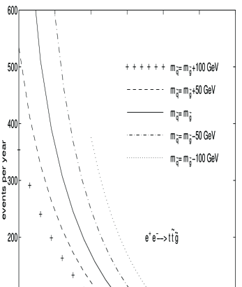
Figure 8.

Number of events per year for $e^{+}e^{-}\rightarrow{t}\,\tilde{t}\,\tilde{g}$ at $E_{\rm cm}=1000$ GeV and luminosity $L=5\times{10}^{33}{\rm cm}^{-2}{\rm s}^{-1}$.

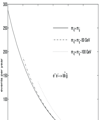
Figure 9.

Number of events per year for $e^{+}e^{-}\rightarrow{b}\,\tilde{b}\,\tilde{g}$ at $E_{\rm cm}=1000$ GeV and luminosity $L=5\times{10}^{33}{\rm cm}^{-2}{\rm s}^{-1}$.

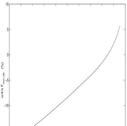
Figure 10.

SU(3) non-oblique corrections for on shell squark decay $\tilde{q}\rightarrow{q}\tilde{g}$.

                                                                                                         

Figure 1: One-loop diagrams for the gqq vertex. The arrow shows the glow of quark number. q̃ can be either $\tilde{q}_{\rm L}$ or $\tilde{q}_{\rm R}$. $F_{\rm Vi}$ corresponds to the correction from diagram (i), ${\rm i}=1,2,3,4$. Similar notations are used in the diagrams below.

                                                                                                         

Figure 2: One-loop diagrams for the qq̃g̃ vertex.

                                                                                                         

Figure 3: One-loop diagrams for g̃ self energies.

                                                                                                         

Figure 4: One-loop diagrams for q self energies.

                                                                                                         

Figure 5: One-loop diagrams for q̃ self energies.

                                                                                                         

Figure 6: One-loop diagrams for g self energies.

                                                                                                         

Figure 7: Feynman diagrams for $\tilde{q}\rightarrow{q}\tilde{g}g$.

                                                                                                         

Figure 8: Number of events per year for $e^{+}e^{-}\rightarrow{t}\,\tilde{t}\,\tilde{g}$ at $E_{\rm cm}=1000$ GeV and luminosity $L=5\times{10}^{33}{\rm cm}^{-2}{\rm s}^{-1}$.

                                                                                                         

Figure 9: Number of events per year for $e^{+}e^{-}\rightarrow{b}\,\tilde{b}\,\tilde{g}$ at $E_{\rm cm}=1000$ GeV and luminosity $L=5\times{10}^{33}{\rm cm}^{-2}{\rm s}^{-1}$.

                                                                                                         

Figure 10: SU(3) non-oblique corrections for on shell squark decay $\tilde{q}\rightarrow{q}\tilde{g}$.

References

- [1] A. Cohen, D. Kaplan, and A. Nelson Phys. Rev. Lett. 78, 2300 (1997).
- [2] G. Dvali and A. Pomarol, Phys. Rev. Lett. 77, 3728 (1996).
- [3] S. Dimopoulos and G. Giudice Phys. Lett. B 357, 573 (1995).
- [4] L. Randall, Nucl. Phys. B 495, 37 (1997).
- [5] H.-C. Cheng, J. Feng, N. Polonsky, Phys. Rev. D 57, 152 (1998).
- [6] D. Pierce, M. Nojiri, and Y. Yamada, SLAC-PUB-7558, in preparation.
- [7] M. Golden and L. Randall, Nucl. Phys. B 361, 3 (1991).
- [8] M. Peskin and T. Takeuchi, Phys. Rev. Lett. 65, 964 (1990).
- [9] M. Peskin and T. Takeuchi, Phys. Rev. D 46, 381 (1992).
- [10] G. Altarelli and R. Barbieri, Phys. Lett. B 253, 161 (1991).
- [11] J. Feng, H. Murayama, M. Peskin, and X. Tata Phys. Rev. D 52, 1418 (1995).
- [12] M. M. Nojiri, K. Fujii, and T. Tsukamoto, Phys. Rev. D 54, 6756 (1996).
- [13] A. Cohen, D. Kaplan, and A. Nelson Phys. Lett. B 388, 588 (1996 ).
- [14] H.-C. Cheng, J. Feng, N. Polonsky, Phys. Rev. D 56, 6875 (1997).
- [15] L. Randall, E. Katz and S. Su,hep-ph/9706478.
- [16] K. Hikasa and Y. Nakamura, hep-ph/9501382.
- [17] M. Peskin, D. Schroeder, “An Introduction to Quantum field Theory”, Addison-Wesley Publishing Company (1995).