LAUR-98-271

Quark Masses, B-parameters, and CP violation parameters $\epsilon$ and $\epsilon^{\prime}/\epsilon$

Rajan Gupta

Group T-8, Mail Stop B-285, Los Alamos National Laboratory

Los Alamos, NM 87545, U. S. A

Email: rajan@qcd.lanl.gov

Abstract

After a brief introduction to lattice QCD, I summarize the results for the light quark masses and the bag parameters $B_{K}$, $B_{6}^{1/2}$, and $B_{8}^{3/2}$. The implications of these results for the standard model estimates of CP violation parameters $\epsilon$ and $\epsilon^{\prime}/\epsilon$ are also discussed.

20 JAN, 1998

1 Introduction

The least well quantified parameters of the Standard Model (SM) are the masses of light quarks and the $\rho$ and $\eta$ parameters in the Wolfenstein representation of the CKM mixing matrix. A non-zero value of $\eta$ signals CP violation. The important question is whether the CKM ansatz explains all observed CP violation. This can be addressed by comparing the SM estimates of the two CP violating parameters $\epsilon$ and $\epsilon^{\prime}/\epsilon$ against experimental measurements. The focus of this talk is to evaluate the dependence of these parameters on the light quark masses and on the bag parameters $B_{K}$, $B_{6}^{1/2}$, and $B_{8}^{3/2}$. I will therefore provide a status report on the estimates of these quantities from lattice QCD (LQCD).

Since this is the only lecture presenting results obtained using LQCD at this school/workshop, I have been asked to give some introduction to the subject. The only way I can cover my charter, introduce LQCD, summarize the results, and make contact with phenomenology is to skip details. I shall try to overcome this shortcoming by giving adequate pointers to relevant literature.

2 Lattice QCD

LQCD calculations are a non-perturbative implementation of field theory using the Feynman path integral approach. The calculations proceed exactly as if the field theory was being solved analytically had we the ability to do the calculations. The starting point is the partition function in Euclidean space-time

$$Z\ =\ \int{\cal D}A_{\mu}\ {\cal D}\psi\ {\cal D}\overline{\psi}\ e^{-S}$$ (1)

where $S$ is the QCD action

$$S\ =\ \int d^{4}x\ \big{(}{1\over 4}F_{\mu\nu}F^{\mu\nu}-\overline{\psi}M\psi\big{)}\ .$$ (2)

and $M$ is the Dirac operator. The fermions are represented by Grassmann variables $\psi$ and $\overline{\psi}$. These can be integrated out exactly with the result

$$Z\ =\ \int{\cal D}A_{\mu}\ {\rm det}M\ e^{\int d^{4}x\ (-{1\over 4}F_{\mu\nu}F^{\mu\nu})}.$$ (3)

The fermionic contribution is now contained in the highly non-local term ${\rm det}M$, and the partition function is an integral over only background gauge configurations. One can write the action, after integration over the fermions, as $S\ ={S_{gauge}+S_{quarks}}=\ \int d^{4}x\ \big{(}{1\over 4}F_{\mu\nu}F^{\mu\nu}\big{)}-\sum_{i}{\rm Ln}({\rm Det}M_{i})$ where the sum is over the quark flavors distinguished by the value of the bare quark mass. Results for physical observables are obtained by calculating expectation values

$$\langle{\cal O}\rangle\ =\ {1\over Z}\int{\cal D}A_{\mu}\ {\cal O}\ e^{-S}\ .$$ (4)

where ${\cal O}$ is any given combination of operators expressed in terms of time-ordered products of gauge and quark fields. The quarks fields in ${\cal O}$ are, in practice, re-expressed in terms of quark propagators using Wick’s theorem for contracting fields. In this way all dependence on quarks as dynamical fields is removed. The basic building block for the fermionic quantities, the Feynman propagator, is given by

$$S_{F}(y,j,b;x,i,a)\ =\ \big{(}M^{-1}\big{)}^{y,j,b}_{x,i,a}\,,$$ (5)

where $M^{-1}$ is the inverse of the Dirac operator calculated on a given background field. A given element of this matrix $\big{(}M^{-1}\big{)}^{y,j,b}_{x,i,a}$ is the amplitude for the propagation of a quark from site $x$ with spin-color $i,a$ to site-spin-color $y,j,b$.

So far all of the above is standard field theory. The problem we face in QCD is how to actually calculate these expectation values and how to extract physical observables from these. I will illustrate the second part first by using as an example the mass and decay constant of the pion.

Consider the 2-point correlation function, $\langle 0|\sum_{x}{\cal O}_{f}(\vec{x},t){\cal O}_{i}(\vec{0},0)|0\rangle$, where the operators ${\cal O}$ are chosen to be the fourth component of the axial current ${\cal O}_{f}={\cal O}_{i}=A_{4}=\overline{\psi}\gamma_{4}\gamma_{5}\psi$ as these have a large coupling to the pion. The 2-point correlation function then gives the amplitude for creating a state with the quantum numbers of the pion out of the vacuum at space-time point $0$ by the “source” operator ${\cal O}_{i}$; the evolution of this state to the point $(\vec{x},t)$ via the QCD Hamiltonian; and finally the annihilation by the “sink” operator ${\cal O}_{f}$ at $(\vec{x},t)$. The rules of quantum mechanics tell us that ${\cal O}_{i}$ will create a state that is a linear combination of all possible eigenstates of the Hamiltonian that have the same quantum numbers as the pion, $i.e.$ the pion, radial excitations of the pion, three pions in $J=0$ state, $\ldots$. The second rule is that on propagating for Euclidean time $t$, a given eigenstate with energy $E$ picks up a weight $e^{-Et}$. Thus, the 2-point function can be written in terms of a sum over all possible intermediate states

$$\langle 0|\sum_{x}{\cal O}_{f}(\vec{x},t){\cal O}_{i}(0)|0\rangle=\sum_{n}{\langle 0|{\cal O}_{f}|n\rangle\langle n|{\cal O}_{i}|0\rangle\over 2E_{n}}\ e^{-E_{n}t}\,.$$ (6)

To study the properties of the pion at rest we need to isolate this state from the sum over $n$. To do this, the first simplification is to use the Fourier projection $\sum_{\vec{x}}$ as it restricts the sum over states to just zero-momentum states, so $E_{n}\to M_{n}$. (Note that it is sufficient to make the Fourier projection over either ${\cal O}_{i}$ or ${\cal O}_{f}$.) The second step to isolate the pion, $i.e.$ project in the energy, consists of a combination of two strategies. One, make a clever choice of the operators ${\cal O}_{i}$ to limit the sum over states to a single state (the ideal choice is to set ${\cal O}_{i}$ equal to the quantum mechanical wave-function of the pion), and two, examine the large $t$ behavior of the 2-point function where only the contribution of the lowest energy state that couples to ${\cal O}_{i}$ is significant due to the exponential damping. Then

$$\langle 0|\sum_{x}{\cal O}_{f}(x,t){\cal O}_{i}(0)|0\rangle\ \ \mathrel{\raise 2.0pt\hbox to24.0pt{\raise-8.0pt\hbox{$t\to\infty$}\hss{$=$}}}\ \ \ \ {\langle 0|{\cal O}_{f}|\pi\rangle\langle\pi|{\cal O}_{i}|0\rangle\over 2M_{\pi}}\ e^{-M_{\pi}t}\,.$$ (7)

The right hand side is now a function of the two quantities we want since $\langle 0|A_{4}|\pi\rangle=M_{\pi}f_{\pi}$. In this way, the mass and the decay constant are extracted from the rate of exponential fall-off in time and from the amplitude.

Let me now illustrate how the left hand side is expressed in terms of the two basic quantities we control in the path integral – the gauge fields and the quark propagator. Using Wick contractions, the correlation function can be written in terms of a product of two quark propagators $S_{F}$,

$$\langle 0|\sum_{x}\overline{\psi}\gamma_{4}\gamma_{5}\psi(x,t)\overline{\psi}\gamma_{4}\gamma_{5}\psi(0,0)|0\rangle\ \equiv\ \langle 0|\sum_{x}S_{F}(0;\vec{x},t)\gamma_{4}\gamma_{5}S_{F}(\vec{x},t;0)\gamma_{4}\gamma_{5}|0\rangle.$$ (8)

This correlation function is illustrated in Fig. 1. It is important to note that one recovers the 2-point function corresponding to the propagation of the physical pion only after the functional integral over the gauge fields, as defined in Eq. 4, is done. To illustrate this Wick contraction procedure further, consider using gauge invariant non-local operators, for example using ${\cal O}=\overline{\psi}(x,t)\gamma_{4}\gamma_{5}({\cal P}e^{\int^{y}_{x}dzigA_{\mu}(z)})\psi(y,t)$ where ${\cal P}$ stands for path-ordered. After Wick contraction the correlation function reads

$$\langle 0|\sum_{x}S_{F}(0;\vec{x},t)\gamma_{4}\gamma_{5}({\cal P}e^{\int^{x}_{z}igA_{\mu}})S_{F}(\vec{z},t;\vec{y},0)\gamma_{4}\gamma_{5}({\cal P}e^{\int^{y}_{0}igA_{\mu}})|0\rangle.$$ (9)

and involves both the gauge fields and quark propagators. This correlation function would have the same long $t$ behavior as shown in Eq. 6, however, the amplitude will be different and consequently its relation to $f_{\pi}$ will no longer be simple. The idea of improving the projection of ${\cal O}$ on to the pion is to construct a suitable combination of such operators that approximates the pion wave-function.

     

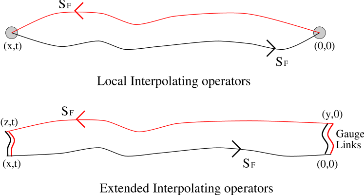
Figure 1: A schematic of the pion 2-point correlation function for local and non-local interpolating operators.

To implement such calculations of correlation functions requires the following steps. A way of generating the background gauge configurations and calculating the action $S$ associated with each; calculating the Feynman propagator on such background fields; constructing the desired correlation functions; doing the functional integral over the gauge fields to get expectation values; making fits to these expectation values, say as a function of $t$ as in Eq. 6 to extract the mass and decay constant; and finally including any renormalization factors needed to properly define the physical quantity. It turns out that at present the only first principles approach that allows us to perform these steps is LQCD. Pedagogical expose to LQCD can be found in [1, 2, 3, 4], and I shall only give a very brief description here.

Lattice QCD – QCD defined on a finite space-time grid – serves two purposes. One, the discrete space-time lattice serves as a non-perturbative regularization scheme. At finite values of the lattice spacing $a$, which provides the ultraviolet cutoff, there are no infinities. Furthermore, renormalized physical quantities have a finite well behaved limit as $a\to 0$. Thus, in principle, one could do all the standard perturbative calculations using lattice regularization, however, these calculations are far more complicated and have no advantage over those done in a continuum scheme. The pre-eminent utility of transcribing QCD on the lattice is that LQCD can be simulated on the computer using methods analogous to those used in Statistical Mechanics. These simulations allow us to calculate correlation functions of hadronic operators and matrix elements of any operator between hadronic states in terms of the fundamental quark and gluon degrees of freedom following the steps discussed above.

The only tunable input parameters in these simulations are the strong coupling constant and the bare masses of the quarks. Our belief is that these parameters are prescribed by some yet more fundamental underlying theory, however, within the context of the standard model they have to be fixed in terms of an equal number of experimental quantities. This is what is done in LQCD. Thereafter all predictions of LQCD have to match experimental data if QCD is the correct theory of strong interactions.

A summary of the main points in the calculations of expectation values via simulations of LQCD are as follows.

• The Yang-Mills action for gauge fields and the Dirac operator for fermions has to be transcribed on to the discrete space-time lattice in such a way as to preserve all the key properties of QCD – confinement, asymptotic freedom, chiral symmetry, topology, and a one-to-one relation between continuum and lattice fields. This step is the most difficult, and even today we do not have a really satisfactory lattice formulation that is chirally symmetric in the $m_{q}=0$ limit and preserves the one-to-one relation between continuum and lattice fields, $i.e.$ no doublers. In fact, the Nielson-Ninomiya theorem states that for a translationally invariant, local, hermitian formulation of the lattice theory one cannot simultaneously have chiral symmetry and no doublers [5]. One important consequence of this theorem is that, in spite of tremendous effort, there is no viable formulation of chiral fermions on the lattice. For a review of the problems and attempts to solve them see [6, 7, 8].

  A second problem is encountered when approximating derivatives in the action by finite differences. As is well known this introduces discretization errors proportional to the lattice spacing $a$. These errors can be reduced by either using higher order difference schemes with coefficients adjusted to take into account effects of renormalization, or equivalently, by adding appropriate combinations of irrelevant operators to the action that cancel the errors order by order in $a$. The various approaches to improving the fermion and gauge actions are discussed in [9, 10, 11]. Here I simply list the three most frequently used discretizations of the Dirac action – Wilson [12], Sheikholeslami-Wohlert (clover) [13], and staggered [14], which have errors of $O(a)$, $O(\alpha_{s}a)-O(a^{2})$ depending on the value of the coefficient of the clover term, and $O(a^{2})$ respectively. The important point to note is that while there may not yet exist a perfect action (no discretization errors) for finite $a$, improvement of the action is very useful but not necessary. Even the simplest formulation, Wilson’s original gauge and fermion action [12], gives the correct results in the $a=0$ limit. It is sufficient to have the ability to reliably extrapolate to $a=0$ to quantify and remove the discretization errors.

• The Euclidean action $S=\int d^{4}x(\ {1\over 4}F_{\mu\nu}F^{\mu\nu}-{\rm TrLn}M)$ for QCD at zero chemical potential is real and bounded from below. Thus $e^{-S}$ in the path integral is analogous to the Boltzmann factor in the partition function for statistical mechanics systems, $i.e.$ it can be regarded as a probability weight for generating configurations. Since $S$ is an extensive quantity the configurations that dominate the functional integral are those that minimize the action. The “importance sampled” configurations (configurations with probability of occurrence given by the weight $e^{-S}$) can be generated by setting up a Markov chain in exact analogy to say simulations of the Ising model. For a discussion of the methods used to update the configurations see [1] or the lectures by Creutz and Sokal in [2].

• The correlation functions are expressed as a product of quark propagators and path ordered product of gauge fields using Wick contractions. This part of the calculation is standard field theory. The only twist is that the calculation is done in Euclidean space-time.

• For a given background gauge configuration, the Feynman quark propagator is a matrix labeled by three indices – site, spin and color. A given element of this matrix gives the amplitude for the propagation of a quark with some spin, color, and space-time point to another space-time point, spin, and color. Operationally, it is simply the inverse of the Dirac operator. Once space-time is made discrete and finite, the Dirac matrix is also finite and its inverse can be calculated numerically. The gauge fields live on links between the sites with the identification $U_{\mu}(x,x+\hat{\mu})=e^{iagA_{\mu}(x+\hat{\mu}/2)}$, $i.e.$ the link at site $x$ in the $\mu$ direction is an SU(3) matrix $U_{\mu}(x,x+\hat{\mu})$ denoting the average gauge field between $x$ and $x+\hat{\mu}$ and labeled by the point $x+\hat{\mu}/2$. Also $U_{\mu}(x,x-\hat{\mu})\equiv U^{\dagger}_{\mu}(x-\hat{\mu},x)$. The links and propagators can be contracted to form gauge invariant correlation functions as discussed above in the case of the pion.

• On the “importance sampled” configurations, the expectation values reduce to simple averages of the correlation functions. The problem is that the set of background gauge configurations is infinite. Thus, while it is possible to calculate the correlation functions for specified background gauge configurations, doing the functional integral exactly is not feasible. It is, therefore, done numerically using monte carlo methods.

The simplest way to understand the numerical aspects of LQCD calculations is to gain familiarity with the numerical treatment of any statistical mechanics system, for example the Ising model. The differences are: (i) the degrees of freedom in LQCD are much more complicated – SU(3) link matrices rather than Ising spins, and quark propagators given by the inverse of the Dirac operator; (ii) The action involves the highly nonlocal term ${\rm Ln\ Det\ }M$ which makes the update of the gauge configurations very expensive; and (iii) the correlation functions are not simple products of spin variables like the specific heat or magnetic susceptibility, but complicated functions of the link variables and quark propagators.

The subtleties arising due to the fact that LQCD is a renormalizable field theory and not a classical statistical mechanics system come into play in the behavior of the correlation functions as the lattice spacing $a$ is varied, and in the quantum corrections that renormalize the input parameters (quark and gluon masses and fields) and the composite operators used in the study of correlation functions. At first glance it might seem that one has introduced an additional parameter in LQCD, the lattice spacing $a$, however, recall that the coupling $\alpha_{s}$ and the cutoff $a$ are not independent quantities but are related by the renormalization group

$$\Lambda_{QCD}={1\over a}e^{-1/2\beta_{0}g^{2}(a)}\ \big{(}\beta_{0}g^{2}(a)\big{)}^{-\beta_{1}/2\beta_{0}^{2}}+\ldots\ ,$$ (10)

where $\Lambda_{QCD}$ is the non-perturbative scale of QCD, and $\beta_{0}=(11-2n_{f}/3)/16\pi^{2}$ and $\beta_{1}=(102-38n_{f}/3)/(16\pi^{2})^{2}$ are the first two, scheme independent, coefficients of the $\beta$-function. In statistical mechanics systems, the lattice spacing $a$ is a physical quantity – the intermolecular separation. In QFT it is simply the ultraviolet regulator that must eventually be taken to zero keeping physical quantities, like the renormalized coupling, spectrum, etc, fixed.

The reason that lattice results are not exact is because in numerical simulations we have to make a number of approximations. The size of these is dictated by the computer power at hand. They are being improved steadily with computer technology, better numerical algorithms, and better theoretical understanding. To evaluate the reliability of current lattice results, it is important to understand the size of the various systematic errors and what is being done to control them. I, therefore, consider it important to discuss these next before moving on to results.

3 Systematic Errors in Lattice Results

The various sources of errors in lattice calculations are as follows.

Statistical errors: The monte carlo method for doing the functional integral employs statistical sampling. The results, therefore, have statistical errors. The current understanding, based on agreement of results from ensembles generated using different algorithms and different initial starting configuration in the Markov process, is that the functional integral is dominated by a single global minimum. Also, configurations with non-trivial topology are properly represented in an ensemble generated using a Markov chain based on small changes to link variables. Another way of saying this is that the data indicate that the energy landscape is simple. As a result, the statistical accuracy can be improved by simply generating more statistically independent configurations with current update methods.

Finite Size errors: Using a finite space-time volume with (anti-)periodic boundary conditions introduces finite size effects. On sufficiently large lattices these effects can be analyzed in terms of interactions of the particle with its mirror images. Lüscher has shown that in this regime these effects vanish exponentially [15]. Current estimates indicate that for $L\mathrel{\raise 2.0pt\hbox to8.0pt{\raise-5.0pt\hbox{$\sim$}\hss{$>$}}}3$ fermi and $M_{\pi}L\geq 6$ the errors are $\mathrel{\raise 2.0pt\hbox to8.0pt{\raise-5.0pt\hbox{$\sim$}\hss{$<$}}}1\%$, and decrease exponentially with increasing $L$.

Discretization errors: The discretization of the Euclidean action on a finite discrete lattice with spacing $a$ leads, in general, to errors proportional to $a$, $\alpha_{s}^{n}a$, $a^{2}$, $\ldots$. The precise form of the leading term depends on the choice of the lattice action and operators [16]. For example, lattice artefacts in the fermion action modify the quark propagator $M^{-1}$ at large $p$ from its continuum form. Numerical data show that the coefficients of the leading term are large, consequently the corrections for $1/a\approx 2{\rm GeV}$ are significant in many quantities, 10-30% [17]. The reliability of lattice results, with respect to $O(a)$ errors, is being improved by a two pronged strategy. First, for a given action extrapolations to the continuum limit $a=0$ are performed by fitting data at a number of values of $a$ using leading order corrections. Second, these extrapolations are being done for different types of actions (Wilson, Clover, staggered) that have significantly different discretization errors. We consider the consistency of the results in the $a=0$ limit as a necessary check of the reliability of the results.

Extrapolations in Light Quark Masses: The physical $u$ and $d$ quark masses are too light to simulate on current lattices. For $1/a=2$ ${\rm GeV}$, realistic simulations require $L/a\mathrel{\raise 2.0pt\hbox to8.0pt{\raise-5.0pt\hbox{$\sim$}\hss{$>$}}}90$ to avoid finite volume effects, $i.e.$ keeping $\tilde{M}_{\pi}L\geq 6$ where $\tilde{M}_{\pi}$ is the lightest pseudoscalar meson mass on the lattice. Current best lattice sizes are $L/a=32$ for quenched and $L/a=24$ for unquenched. Thus, to get results for quantities involving light quarks, one typically extrapolates in $m_{u}=m_{d}$ from the range $m_{s}/3-2m_{s}$ using simple polynomial fits based on chiral perturbation theory. For quenched simulations there are additional problems for $m_{q}\mathrel{\raise 2.0pt\hbox to8.0pt{\raise-5.0pt\hbox{$\sim$}\hss{$<$}}}m_{s}/3$ as discussed below in the item on quenching errors.

Discretization of heavy quarks: Simulations of heavy quarks ($c$ and $b$) have discretization errors of $O(ma)$ and $O(pa)$. This is because quark masses measured in lattice units, $m_{c}a$ and $m_{b}a$, are of order unity for $2{\rm GeV}\leq 1/a\leq 5{\rm GeV}$. It turns out that these discretization errors are large even for $m_{c}$. Extrapolations of lattice data from lighter masses to $m_{b}$ using HQET have also not been very reliable as the corrections are again large. The three most promising approaches to control these errors are non-relativistic QCD, $O(a)$ improved heavy Dirac, and HQET. These are discussed in [19, 20, 21]. There will not be any discussion of heavy quark physics in this talk.

Matching between lattice and the continuum (renormalization constants): Experimental data are analyzed using some continuum renormalization scheme like $\overline{MS}$, so results in the lattice scheme have to be converted to this scheme. The perturbative relation between renormalized quantities in say $\overline{MS}$ and the lattice scheme, are in almost all cases, known only to 1-loop. Data show that the $O(\alpha_{s}^{2})$ corrections can be large, $\sim 10-50\%$ depending on the quantity at hand, even after implementation of the improved perturbation theory technique of Lepage-Mackenzie [18]. Recently, the technology to calculate these factors non-perturbatively has been developed and is now being exploited [22]. As a result, the reliance on perturbation theory for these matching factors will be removed.

Operator mixing: The lattice operators that arise in the effective weak Hamiltonian can, in general, mix with operators of the same, higher, and lower dimensions because at finite $a$ the symmetries of the lattice and continuum theories are not the same. Perturbative estimates of this mixing can have an even more serious problem than the uncertainties discussed above in the matching coefficients. In cases where there is mixing with lower dimensional operators, the mixing coefficients have to be known very accurately otherwise the power divergences overwhelm the signal as $a\to 0$. In cases where there is mixing, due to the explicit chiral symmetry breaking in Wilson like actions, with operators of the same dimension but with different tensor structures, the chiral behavior may again be completely overwhelmed by the artefacts. In both of these cases a non-perturbative calculation of the mixing coefficients is essential.

Quenched approximation: The inclusion of the fermionic contribution, ${\rm Ln\ det}(M)$, in the Boltzmann factor $e^{-S}$ for the generation of background gauge configurations increases the computational cost by a factor of $10^{3}-10^{4}$. The strategy, therefore, has been to initially neglect this factor, and to bring all other above mentioned sources of errors under quantitative control. The justification is that the quenched theory retains a number of the key features of QCD – confinement, asymptotic freedom, and the spontaneous breaking of chiral symmetry – and is expected to be good to within $10-20\%$ for a number of quantities. One serious drawback is that the quenched theory is not unitary and $\chi$PT analysis of it shows the existence of unphysical singularities in the chiral limit. For example, the chiral expansions of pseudoscalar masses and decay constants in the quenched theory are modified in two ways. One, the normal chiral coefficients are different in the quenched theory, and second there are additional terms that are artefacts and are singular in the limit $m_{q}=0$ [23, 24]. These artefacts are expected to start becoming significant for $m_{q}\mathrel{\raise 2.0pt\hbox to8.0pt{\raise-5.0pt\hbox{$\sim$}\hss{$<$}}}m_{s}/3$ [25, 26]. Thus, in quenched simulations one of the strategies for extrapolations in the light quark masses is to use fits based on $\chi$PT, keep only the normal coefficients, and restrict the data to the range $m_{s}/3-2m_{s}$ where the artifacts are expected to be small. In this talk I shall use this procedure to “define” the quenched results.

The above mentioned systematic errors are under varying degrees of control depending on the quantity at hand. Of the systematics effects listed above, quenching errors are by far the least well quantified, and are, to first approximation, unknown. Of the remaining sources the two most serious are the discretization errors and the matching of renormalized operators between the lattice and continuum theories. An example of the latter is the connection between the quark mass in lattice scheme and in a perturbative scheme like $\overline{MS}$. We shall discuss the status of control over these errors in more details when discussing data.

4 Light Quark Masses from $\chi$PT

The masses of light quarks cannot directly be measured in experiments as quarks are not asymptotic states. One has to extract the masses from the pattern of the observed hadron spectrum. Three approaches have been used to estimate these – chiral perturbation theory ($\chi$PT), QCD sum-rules, and lattice QCD.

$\chi$PT relates pseudoscalar meson masses to $m_{u}$, $m_{d}$, and $m_{s}$. However, due to the presence of an overall unknown scale in the chiral Lagrangian, $\chi$PT can predict only two ratios amongst the three light quark masses. The current estimates are [27, 28, 29]

	Lowest order	Next order
$2m_{s}/(m_{u}+m_{d})$	$24.2-25.9$	$24.4(1.5)$
$m_{u}/m_{d}$	$0.55$	$0.553(43)$  .

These ratios have been calculated neglecting the Kaplan-Manohar symmetry [30]. The subtle point here is that the masses $\mu_{i}$ extracted from low energy phenomenology are related to the fundamental parameters $m_{i}$, defined at some high scale by the underlying theory, as $\mu_{i}=m_{i}+\beta*\det M/m_{i}\Lambda_{\chi SB}$, where the second, correction, term is an instanton induced additive renormalization. For the $u$ quark, the magnitude of this term is roughly equal to the $\chi$PT estimates of $\mu_{u}$ for $\beta\approx 2$ [31]. Consequently, using $\chi$PT, one cannot estimate the size of isospin breaking from low energy phenomenology alone. At next to leading order, only one combination of ratios ($Q^{2}=(m_{s}^{2}-\hbox{$\overline{m}$}^{2})/(m_{d}^{2}-m_{u}^{2})$ as defined in [29]) can be determined unambiguously from $\chi$PT. Even if one ignores the Kaplan-Manohar subtlety (such an approach has been discussed by Leutwyler under the assumption that the higher order terms are small [29]) one still needs input from sum-rules or LQCD to get absolute values of quark masses.

5 Light Quark Masses from LQCD

The most extensive and reliable results from LQCD have been obtained in the quenched approximation. In the last year the statistical quality of the quenched data has been improved dramatically especially by the work of the two Japanese Collaborations CP-PACS and JLQCD (see [32] for a recent review). Simultaneously, the lattice sizes have been pushed to $\mathrel{\raise 2.0pt\hbox to8.0pt{\raise-5.0pt\hbox{$\sim$}\hss{$>$}}}3$ fermi for the lattice spacing in the range $0.5-0.25$ ${\rm GeV}^{-1}$. In Fig. 2 we show the CP-PACS data obtained using Wilson fermions. To highlight the statistical improvement we show data at $\beta=6.0$ from the next best calculation (with respect to both statistics and lattice size) [33].

To reliably extrapolate the lattice data to the continuum limit one needs control over discretization errors and over the matching relations between the lattice scheme and the continuum scheme, say $\overline{\rm MS}$. The first issue has been addressed by the community by simulating three different discretizations of the Dirac action – Wilson, SW clover, and staggered – which have discretization errors of $O(a)$, $O(\alpha_{s}(a)a)$, and $O(a^{2})$ respectively. The second issue, reliability of the 1-loop perturbative matching relations, is being checked by using non-perturbative estimates.

For Wilson and SW clover formulations, the internal consistency of the lattice calculations can be checked by calculating the quark masses two different ways. The first is based on methods of $\chi$PT, $i.e.$ the calculated hadron masses are expressed as functions of the quark masses as in $\chi$PT. This method, based on hadron spectroscopy, is labeled HS for brevity. In the second method, labeled WI, quark masses are defined using the ward identity $\partial_{\mu}\overline{\psi}\gamma_{5}\gamma_{\mu}\psi=(m_{1}+m_{2})\overline{\psi}\gamma_{5}\psi$. An example of such checks is shown in Fig. 2. The solid lines are fits to the HS and WI estimates using the Wilson action and on the same statistical sample of configurations. The very close agreement of the extrapolated values is probably fortuitous since the linear extrapolation in $a$, shown in Fig. 2, neglects both the higher order discretization errors and the $O(\alpha_{s}(a)^{2})$ errors in the 1-loop perturbative matching relations. The figure also shows preliminary results for the same WI data but now with non-perturbative Z’s. The correction is large, note the large change in the slope in $a$, yet the extrapolated value is $\mathrel{\raise 2.0pt\hbox to8.0pt{\raise-5.0pt\hbox{$\sim$}\hss{$<$}}}4$ ${\rm MeV}$. The final analysis using non-perturbative Z’s will be available soon, and it is unlikely that the central value presented below will shift significantly.

     

Figure 2: Linear extrapolation of $\overline{m}$ versus $a(M_{\rho})$ for Wilson fermions using HS and WI methods. The WI data corrected by using non-perturbative estimates for the matching constants are also shown.

Lastly, in the quenched approximation, estimates of quark masses can and do depend on the hadronic states used to fix them. The estimates of $\overline{m}$ given below were extracted using the pseudoscalars mesons, $i.e.$ pions, with the scale $a$ set by $M_{\rho}$. Using either the nucleon or the $\Delta$ to fix $\overline{m}$ would give $\sim 10\%$ smaller estimates. Similarly, extracting $m_{s}$ using $M_{K}$ gives estimates that are $\sim 20\%$ smaller that those using $M_{K^{*}}$ or $M_{\phi}$ as shown below. While these estimates of quenching errors are what one would expect naively, we really have to wait for sufficient unquenched data to quantify these more precisely.

A summary of the quenched results in ${\rm MeV}$at scale $\mu=2\ {\rm GeV}$, based on an analysis of the 1997 world data [32], is

	Wilson	TI Clover	Staggered
$\hbox{$\overline{m}$}(M_{\pi})$	$4.1(1)$	$3.8(1)$	$3.5(1)$
$m_{s}(M_{K})$	$107(2)$	$99(3)$	$91(2)$
$m_{s}(M_{\phi})$	$139(11)$	$117(8)$	$109(5)$ .

The difference in estimates between Wilson, tadpole improved (TI) clover, and staggered results could be due to the neglected higher order discretization errors and/or due to the difference between non-perturbative and 1-loop estimates of $Z$’s. This uncertainty is currently $\approx 15\%$. Similarly, the $\approx 20\%$ variation in $m_{s}$ with the state used to extract it, $M_{K}$ versus $M_{K^{*}}$ (or equivalently $M_{\phi}$) could be due to the quenched approximation or again an artifact of keeping only the lowest order correction term in the extrapolations. To disentangle these discretization and quenching errors we again need precise unquenched data.

Thus, for our best estimate of quenched results we average the data and use the spread as the error. To these, we add a second uncertainty of $10\%$ as due to the determination of the scale $1/a$ (another estimate of quenching errors). The final results, in $\overline{\rm MS}$ scheme evaluated at $2$ GeV, are [32]

$$\overline{m} = 3.8(4)(4)\ {\rm MeV}$$

$$m_{s} = 110(20)(11)\ {\rm MeV}\,.$$ (11)

The important question is how do these estimates change on unquenching. The 1996 analyses suggested that unquenching could lower the quark masses by $\approx 20\%$ [34, 35], however, as discussed in [32] I no longer feel confident making an assessment of the magnitude of the effect. The data does still indicate that the sign of the effect is negative, $i.e.$ that unquenching lowers the masses. An estimate of the size requires more unquenched data.

To end this section let me comment on a comparison of the quenched estimates with values extracted from sum-rules as there seems to be a general feeling that the two estimates are vastly different. In fact the recent analyses indicate that the quenched lattice results and the sum-rule estimates are actually consistent. A large part of the apparent difference is due to the use of different scales at which results are presented. Lattice QCD results are usually stated at $\mu=2\ {\rm GeV}$, while the sum-rules community uses $\mu=1\ {\rm GeV}$, and the running of the masses between these two scales is an $\approx 30\%$ effect in full QCD. This issue is important enough that I would like to briefly review the status of sum-rule estimates.

6 Sum rule determinations of $\overline{m}$ and $m_{s}$

A summary of light quark masses from sum-rules is given in Table 1. Sum rule calculations proceed in one of two ways. (i) Using axial or vector current Ward identities one writes a relation between two 2-point correlation functions. One of these is evaluated perturbatively after using the operator product expansion, and the other by saturating with intermediate hadronic states [36, 37]. The quark masses are the constant of proportionality between these two correlation functions. (ii) Evaluating a given correlation function both by saturating with known hadronic states and by evaluating it perturbatively [38]. The perturbative expression depends on quark masses, and defines the renormalization scheme in which they are measured. The main sources of systematic errors arise from using (i) finite order calculation of the perturbative expressions, and (ii) the ansatz for the hadronic spectral function. Of these the most severe is the second as there does not exist enough experimental data to constrain the spectral function even for $\mu<2$ GeV. Since there are narrow resonances in this region, one cannot match the two expressions point by point in energy scale. The two common approaches are to match the moments integrated up to some sufficiently high scale (finite energy sum rules) or to match the Borel transforms. The hope then is that the result is independent of this scale or of the Borel parameter.

reference	$\overline{m}$ (MeV)	$m_{s}$ (MeV)
[39] 1989	${}=6.2(0.4)$	${}=138(8)$
[36] 1995	${}=4.7(1.0)$
[38] 1995	${}=5.1(0.7)$	${}=144(21)$
[37] 1995		${}=137(23)$
[40] 1996		${}=148(15)$
[41] 1997		${}=91-116$
[42] 1997		${}=115(22)$
[43] 1997	${}=4.9(1.9)$
[45] 1997	${}\geq 3.8-6$	${}\geq 118-189$
[46] 1997	${}\geq 3.4$	${}\geq 88(9)$
[47] 1997	${}\geq 4.1-4.4$	${}\geq 104-116$

Table 1: Values and bounds on $\overline{m}$ and $m_{s}$, in $\overline{\rm MS}$ scheme at 2 GeV, from sumrule analyses.

Progress in sum-rules analyses has also been incremental as in LQCD. The perturbative expressions have now been calculated to $O(\alpha_{s}^{3})$ [40], and the value of $\Lambda_{QCD}^{(3)}$ has settled at $\approx 380{\rm MeV}$. A detailed analysis of the convergence of the perturbation expansion suggests that the error associated with the truncation at $O(\alpha_{s}^{3})$ is $\approx 10\%$ for $\mu\geq 2$ GeV [40].

Improving the spectral function has proven to be much harder. For example, Colangelo et al. [41] have extended the analysis of $m_{s}$ in [37, 40] by constructing the hadronic spectral function up to the first resonance ($K^{*}(1430)$) from known $K\pi$ phase shift data. Similarly, Jamin [42] has used a different parametrization of the Omnes representation of the scalar form factor using the same phase shift data. In both cases the reanalysis lowers the estimate of the strange quark mass significantly. The new estimates, listed in Table 1, are consistent with the quenched estimates discussed in Section 5.

One can circumvent the uncertainties in the ansatz for the spectral function by deriving rigorous lower bounds using just the positivity of the spectral function [44, 45, 46, 47]. Of these the most stringent are in [47] which rule out $\hbox{$\overline{m}$}<3$ and $m_{s}<80$ ${\rm MeV}$ for $\mu\mathrel{\raise 2.0pt\hbox to8.0pt{\raise-5.0pt\hbox{$\sim$}\hss{$<$}}}2.5$ GeV. The bounds, however, have a significant dependence on the scale $\mu$ as evident by comparing the above values to those in the last row in Table 1, and the open question is how to fix $\mu$, $i.e.$ the upper limit of integration in the finite energy sum rules at which duality between PQCD and hadronic physics becomes valid? Unfortunately, this question cannot be answered ab initio.

7 Implications for $\epsilon^{\prime}/\epsilon$

The Standard Model (SM) prediction of $\epsilon^{\prime}/\epsilon$ can be written as [48]

$$\epsilon^{\prime}/\epsilon=A\bigg{\{}c_{0}+\big{[}c_{6}B_{6}^{1/2}+c_{8}B_{8}^{3/2}\big{]}M_{r}\bigg{\}}\ ,$$ (12)

where $M_{r}=(158{\rm MeV}/(m_{s}+m_{d}))^{2}$ and all quantities are to be evaluated at the scale $m_{c}=1.3{\rm GeV}$. Eq. 12 highlights the dependence on the light quark masses and the bag parameters $B_{6}^{1/2}$ and $B_{8}^{3/2}$. For the other SM parameters that are needed in obtaining this expression we use the central values quoted by Buras et al. [48]. Then, we get $A=1.29\times 10^{-4}$, $c_{0}=-1.4$, $c_{6}=7.9$, $c_{8}=-4.0$. Thus, to a good approximation $\epsilon^{\prime}/\epsilon\propto M_{r}$.

Conventional analysis, with $m_{s}+m_{d}=158{\rm MeV}$ and $B_{6}^{1/2}=B_{8}^{3/2}=1$, gives $\epsilon^{\prime}/\epsilon\approx 3.2\times 10^{-4}$. The uncertainties in the remaining SM parameters used to determine $A,c_{0},c_{6},$ and $c_{8}$ in Eq. 12 are large enough that, in fact, any value between $-1\times 10^{-4}$ and $16\times 10^{-4}$ is acceptable[48]. Current experimental estimates are $7.4(5.9)\times 10^{-4}$ from Fermilab E731 [49] and $23(7)\times 10^{-4}$ from CERN NA31 [50]. So at present there is no resolution of the issue whether the CKM ansatz explains all observed CP violation.

The new generation of experiments, Fermilab E832, CERN NA48, and DA$\Phi$NE KLOE, will reduce the uncertainty to $\approx 1\times 10^{-4}$. First results from these experiments should be available in the next couple of years. Thus, it is very important to tighten the theoretical prediction.

As is clear from Eq. 12, both the values of quark masses and the interplay between $B_{6}^{1/2}$ and $B_{8}^{3/2}$ will have a significant impact on $\epsilon^{\prime}/\epsilon$. The lower values of quark masses suggested by lattice QCD analyses would increase the estimate. The status of results for the various B-parameters relevant to the study of CP violation are discussed in the next section.

8 B-parameters, $B_{K}$, $B_{6}$, $B^{3/2}_{7}$, $B^{3/2}_{8}$

Considerable effort has been devoted by the lattice community to calculate the various B-parameters needed in the standard model expressions describing CP violation. A summary of the results and the existing sources of uncertainties are as follows.

8.1 $B_{K}$

The standard model expression for the parameter $\epsilon$, which characterizes the strength of the mixing of CP odd and even states in $K_{L}$ and $K_{S}$, is of the form  [51]

$$|\epsilon|\sim{\rm Im}(V_{td}V_{ts}^{*})B_{K}(\mu)\ \Phi\big{(}{m_{c}\over M_{W}},{m_{t}\over M_{W}},\mu\big{)}\ ,$$ (13)

where $\Phi$ is a known function involving Inami-Lim functions and CKM elements. This relation provides a crucial constraint in the effort to pin down the $\rho$ and $\eta$ parameters in the Wolfenstein parameterization of the CKM matrix  [52]. The quantity $B_{K}$ parameterizes the QCD corrections to the basic box diagram responsible for $K^{0}-\overline{K^{0}}$ mixing. This transition matrix element is what we calculate on the lattice.

The calculation of $B_{K}$ is one of the highlights of LQCD simulations. It was one of the first quantities for which theoretical estimates were made, using quenched chiral perturbation theory, of the lattice size dependence, dependence on quark masses, and on the effects of quenching [53, 54, 26, 55]. Numerical data in the staggered formulation (which has the advantage of retaining a chiral symmetry which preserves the continuum like behavior of the matrix elements) is consistent with these estimates in both the sign and the magnitude. Since all these corrections have turned out to be small, results for $B_{K}$ with staggered fermions have remained stable over the last five years.

Three collaborations have pursued calculations of $B_{K}$ using staggered fermions. The results are $B_{K}(NDR,2\ {\rm GeV})=0.62(2)(2)$ by Kilcup, Gupta, and Sharpe [55], $0.552(7)$ by Pekurovsky and Kilcup [56], and $0.628(42)$ by the JLQCD collaboration[57]. Of these, the results by the JLQCD collaboration are based on a far more extensive analysis. The quality of their data are precise enough to include both the leading $O(a^{2})$ discretization corrections, and the $O(\alpha_{s}^{2})$ corrections in the 1-loop matching factors. Their data, along with the extrapolation to $a=0$ limit including both factors, are shown in Fig. 3. I consider theirs the current best estimate of the quenched value.

     

Figure 3: JLQCD data for $B_{K}(NDR,2\ {\rm GeV})$, and their extrapolation to the continuum limit keeping both the $O(a^{2})$ discretization corrections, and the $O(\alpha_{s}^{2})$ in the 1-loop matching factors for two different discretizations of the weak operator. The extrapolation of the data without including the $O(\alpha_{s}^{2})$ corrections are shown by the dashed lines.

The two remaining uncertainties in the above estimate of $B_{K}$ are quenching errors and SU(3) breaking effects (all current results have been obtained using degenerate quarks $m_{u}=m_{d}=m_{s}$, with kaons composed of two quarks of mass $\sim m_{s}/2$ instead of $m_{s}$ and $m_{d}$). There exists only preliminary unquenched data [58] which suggest that the effect of sea quarks is to increase the estimate by $\approx 5\%$. Lastly, Sharpe has used $\chi$PT to estimate that the SU(3) breaking effects could also increase $B_{K}$ by another $4-8\%$ [26]. Confirmation of these corrections requires precise unquenched data which is still some years away.

In a number of phenomenological applications what one wants is the renormalization group invariant quantity $\hat{B}_{K}$ defined, at two-loops, as

$$\hat{B}_{K}=B_{K}(\mu)\ \big{(}\alpha_{s}(\mu)\big{)}^{-\gamma_{0}/2\beta_{0}}\big{(}1+{\alpha_{s}(\mu)\over 4\pi}\big{[}{\beta_{1}\gamma_{0}-\beta_{0}\gamma_{0}\over 2\beta_{0}^{2}}\big{]}\big{)}\ .$$ (14)

Unfortunately, to convert the quenched JLQCD number, $0.628(42)$, one has to face the issue of the choice of the value of $\alpha_{s}$ and the number of flavors $n_{f}$. It turns out that the two-loop evolution of $B_{K}$ is such that one gets essentially the same number for the quenched theory, $0.87(6)$ for $n_{f}=0$ and $\alpha_{s}(2GeV)=0.192$, and $0.84(6)$ for the physical case of $n_{f}=3$ and $\alpha_{s}(M_{\tau})=0.354$. One might interpret this near equality to imply that the quenching errors are small. Such an argument is based on the assumption that there exists a perturbative scale at which the full and quenched theories match. Since there is no a priori reason to believe that this is true, my preference is to double the difference and assign a second error of $0.06$, an estimate also suggested by the preliminary unquenched data and the $\chi$PT analysis. With this caveat I arrive at the lattice prediction

$$\hat{B}_{K}=0.86(6)(6).$$ (15)

8.2 $\langle\pi^{+}\pi^{0}|{\cal O}_{4}|K^{+}\rangle$ and its relation to $B_{K}$

The $\Delta S=2$ operator $\overline{s}L_{\mu}d\overline{s}L_{\mu}d$ responsible for the $K^{0}-\overline{K^{0}}$ transition belongs to the same 27 representation of SU(3) as the $\Delta S=1,\Delta I=3/2$ operator ${\cal O}_{4}=\overline{s}L_{\mu}d(\overline{u}L_{\mu}u-\overline{d}L_{\mu}d)+\overline{s}L_{\mu}u\overline{u}L_{\mu}d$. At tree level in $\chi$PT, one gets the relation [59, 60]

$$\langle K^{0}|{\cal O}_{\Delta S=2}|\overline{K^{0}}\rangle={\sqrt{2}f_{\pi}\over 3i}\ {2M_{K}^{2}\over{M_{K}^{2}-M_{\pi}^{2}}}\langle\pi^{+}\pi^{0}|{\cal O}_{4}|K^{+}\rangle$$ (16)

So one way to calculate $B_{K}$ is to measure $\langle\pi^{+}\pi^{0}|{\cal O}_{4}|K^{+}\rangle$ on the lattice and then use Eq. 16. The motivation for doing this is that, for Wilson-like lattice actions, ${\cal O}_{4}$ is only multiplicatively renormalized due to CPS symmetry [61], whereas the $\Delta S=2$ operator mixes with all other chirality operators of dimension six. Using 1-loop values for these mixing coefficients has proven inadequate, though the recent implementation of non-perturbative estimates has made this situation much better [62].

The first lattice calculations of the $\Delta I=3/2$ part of the $K^{+}\to\pi^{+}\pi^{0}$ amplitude [63, 65] gave roughly twice the experimental value, even though the $B_{K}$ extracted from this “wrong” amplitude “agrees” with modern lattice estimates. The important question therefore is how reliable are the $\chi$PT relations between $\langle\pi^{+}\pi^{0}|{\cal O}_{4}|K^{+}\rangle\big{|}_{lattice}$ and $\langle\pi^{+}\pi^{0}|{\cal O}_{4}|K^{+}\rangle\big{|}_{physical}$, and between $\langle\pi^{+}\pi^{0}|{\cal O}_{4}|K^{+}\rangle\big{|}_{lattice}$ and $\langle K^{0}|{\cal O}_{\Delta S=2}|\overline{K^{0}}\rangle$, $i.e.$ does one or both fail?

There are three sources of systematic errors in lattice calculations of $\langle\pi^{+}\pi^{0}|{\cal O}_{4}|K^{+}\rangle$ that could explain the contradiction. The calculation is done in the quenched approximation, on finite size lattices, and with unphysical kinematics (in the lattice calculation the final state pions are degenerate with the kaon since $m_{u}=m_{d}=m_{s}$, and are at rest). Of the three possibilities, the last is the most serious as it gives a factor of two even at the tree-level

$${2M_{K}^{2}\over{M_{K}^{2}-M_{\pi}^{2}}}\langle\pi^{+}\pi^{0}|{\cal O}_{4}|K^{+}\rangle\big{|}_{physical}=\langle\pi^{+}\pi^{0}|{\cal O}_{4}|K^{+}\rangle\big{|}_{unphysical}\ .$$ (17)

This tree-level correction was taken onto account in [63, 65]. The source of the remaining discrepancy by a factor of two was anticipated by Bernard as due to the failure of the tree-level expression [64]. Recently, Golterman and Leung [59] have calculated the 1-loop corrections to Eq. 17. This calculation involves a number of unknown $O(p^{4})$ chiral coefficients of the weak interactions and thus has a number of caveats. However, under reasonable assumptions about the value of these $O(p^{4})$ constants, the corrections due to finite volume, quenching, and unphysical kinematics all go in the right direction, and the total 1-loop correction can modify Eq. 17 by roughly a factor of two. On the other hand the modification to the connection with $B_{K}$ at the physical point is small.

The JLQCD Collaboration [66] has recently updated the calculations in [63, 65]. By improving the statistical errors they are able to validate the trends predicted by 1-loop $\chi$PT expressions. Thus one has a plausible resolution of the problem. I say plausible because the calculation involves a number of unknown chiral couplings in both the full and quenched theory and also because of the size of the 1-loop correction. The conclusive statement is the failure of $\chi$PT for the relation Eq. 17.

The other relevant question is what bearing does the analysis of Golterman and Leung [59] have on the calculations of other $B$-parameters. In the calculation of $B_{K}$, based on measuring the $\langle K^{0}|{\cal O}_{\Delta S=2}|\overline{K^{0}}\rangle$ transition matrix element as discussed in section 8.1, $\chi$PT has been used only to understand effects of finite volume and chiral logs. These are found to be small and the data show the predicted behavior. Based on this success of $\chi$PT we estimate that the two remaining errors – quenching and the use of degenerate quarks – are each $\approx 5\%$ as suggested by 1-loop $\chi$PT. On the other hand, in present calculations of $B_{6}$, $B^{3/2}_{7}$, and $B^{3/2}_{8}$ $\chi$PT is used in an essential way, $i.e.$ to relate $\langle\pi^{+}\pi^{0}|{\cal O}|K^{+}\rangle$ to $\langle\pi^{+}|{\cal O}|K^{+}\rangle$. Second, the calculations are done for unphysical kinematics, $i.e.$ the final state pion is degenerate with the kaon. It would be interesting to know the size of the one-loop corrections to these relations.

8.3 $B^{3/2}_{7}$ and $B^{3/2}_{8}$

Assuming the reduction of $\langle\pi^{+}\pi^{0}|{\cal O}_{7,8}^{\Delta I=3/2}|K^{+}\rangle$ to $\langle\pi^{+}|{\cal O}_{7,8}^{\Delta I=3/2}|K^{+}\rangle$ using tree-level $\chi$PT is reliable, the lattice calculations of $B^{3/2}_{7}$ and $B^{3/2}_{8}$ are as straightforward as those for $B_{K}$. There are three “modern” quenched estimates of $B^{3/2}_{7}$ and $B^{3/2}_{8}$ which supercede all previous reported values. These, in the NDR-$\overline{\rm MS}$ scheme at $2$ ${\rm GeV}$, are

Fermion type	Matching $Z$	$\beta$	$1/a$ GeV	$B^{3/2}_{7}$	$B^{3/2}_{8}$
(A) Staggered [55]	1-loop	$6.0,\ 6.2$	$a\to 0$	$0.62(3)(6)$	$0.77(4)(4)$
(B) Wilson [67]	1-loop	$6.0$	$2.3$	$0.58(2)(7)$	$0.81(3)(3)$
(C) Tree-level Clover [62]	1-loop	$6.0$	$2.0$	$0.58(2)$	$0.83(2)$
(D) Tree-level Clover [62]	Non-pert.	$6.0$	$2.0$	$0.72(5)$	$1.03(3)$ .

where I have also given the type of lattice action used, the $\beta$’s at which the calculation was done, the lattice scale $1/a$ at which the results were extracted, and how the 1-loop matching coefficients were determined.

The difference between (C) and (D) is the use of perturbative versus non-perturbative Z’s. Thus (D) is the more reliable of the APE numbers. The agreement between (B) and (C), in spite of the difference in the action, is a check that the numerics are stable. All three of these results suffer from the fact that these calculations were done at $\beta=6.0$ ($1/a\approx 2$ GeV) and there does not yet exist data at other $\beta$ needed to do the extrapolation to the continuum limit.

The result (A) does incorporate an extrapolation to a=0, but with only two beta values. For example, $B^{3/2}_{8}=1.24(1)$ and $1.03(2)$ at $\beta=6.0$ and $6.2$ respectively. Due to the large slope in $a^{2}$, such an extrapolation based on two points should be considered preliminary. Lastly, one needs to demonstrate that corrections to 1-loop $Z^{\prime}s$ are under control.

8.4 $B_{6}$

The recent work of Pekurovsky and Kilcup [56] provides the best lattice estimate for $B_{6}$. Their results $B_{6}=0.67(4)(5)$ for quenched and $0.76(3)(5)$ for two flavors have the following systematics that are not under control. The calculation is done for degenerate quarks, $m_{u}=m_{d}=m_{s}$ and uses the lowest order $\chi$PT to relate $\langle\pi\pi|{\cal O}|K^{+}\rangle$ to $\langle\pi|{\cal O}|K^{+}\rangle$. There is no reason to believe that higher order corrections may not be as or more significant as discussed above for ${\cal O}_{4}$. The second issue is that the 1-loop perturbative corrections in the matching coefficients are large. Lastly, there is no estimate for the discretization errors as the calculation has been done at only one value of $\beta$. Thus, at this point there is no solid prediction from the lattice.

9 Conclusions and Acknowledgements

In view of the new generation of ongoing experiments to measure $\epsilon^{\prime}/\epsilon$ with the proposed accuracy of $1\times 10^{-4}$, it is very important to firm up the theoretical prediction. The standard model estimate depends very sensitively on the sum $m_{s}+m_{d}$ and on the interplay between the strong and electromagnetic penguin operators, $i.e.$ $B_{6}^{1/2}$ and $B_{8}^{3/2}$. Quenched lattice results for $(m_{s}+m_{d})(2\ {\rm GeV})$ are settling down at $115(25)$ MeV, and preliminary evidence is that unquenching further lowers these estimates. The calculations of $B_{6}^{1/2}$ and $B_{8}^{3/2}$ are less advanced. Hopefully we can provide reliable quenched estimates for these parameters in the next year or so. Thereafter, we shall start to chip away at realistic full QCD simulations.

Acknowledgements

I would like to thank the organizers of CPMASS97 and ORBIS SCIENTIAE’97 for very stimulating conferences, and my collaborators Tanmoy Bhattacharya, Greg Kilcup, and S. Sharpe for many discussions. I also thank the DOE and the Advanced Computing Laboratory for support of our work.

References

- [1] M. Creutz, Quarks, Gluons, and Lattices, Cambridge University Press, 1983
- [2] Quantum Fields on the Computer, Ed. M. Creutz, World Scientific, 1992.
- [3] Quantum Fields on a Lattice, I. Montvay and G. Münster, Cambridge Monographs on
- [4] H. J. Rothe, Quantum Gauge Theories: An Introduction, World Scientific, 1997.
- [5] H.B.Nielsen and M. Ninomiya, .
- [6] Y. Shamir, ; .
- [7] R. Narayanan, hep-lat/9707035.
- [8] M. Testa, hep-lat/9707007.
- [9] M. Alford, T. Klassen, and P. Lepage, ; and hep-lat/9712005
- [10] M. Lüscher, et al., .
- [11] P. Hasenfratz, hep-lat/9709110.
- [12] K. G. Wilson, ; in New Phenomena in Subnuclear Physics (Erice 1975), Ed. A. Zichichi, Plenum New York, 1977.
- [13] B. Sheikholesalami and R. Wohlert, .
- [14] J. Kogut and L. Susskind, ; T. Banks, J. Kogut, and L. Susskind, ; L. Susskind, .
- [15] M. Lüscher, Selected Topics In Lattice Field Theory, Lectures at the 1988 Les Houches summer school, North Holland, 1990.
- [16] K. Symanzik, in Mathematical Problems in Theoretical Physics, Springer Lecture Notes in Physics, bf 153 (1982) 47; M. Lüscher and P. Weisz, it Commun. Math. Phys. 97 1985 59; G. Heatlie, et al., .
- [17] H. Wittig, hep-lat/9710013; M. Peardon, hep-lat/9710029
- [18] P. Lepage and P. Mackenzie, .
- [19] Phys. Rev. D48 (1993) 266 P. Lepage and B. Thacker, ; G. Lepage, L. Magnea, C. Nakhleh, U. Magnea and K. Hornbostel, .
- [20] A. El-Khadra, A. Kronfeld, and P. Mackenzie, .
- [21] M. Neubert, ; G. Martinelli and C. Sachrajda, ; J. Mandula and M. Ogilvie, hep-lat/9703020.
- [22] G.C. Rossi, ; M. Lüscher, et al., ; G. Martinelli, et al., .
- [23] S. Sharpe, , , , .
- [24] C. Bernard and M. Golterman, ; ; ; M. Golterman, hep-lat/9405002 and hep-lat/9411005.
- [25] R. Gupta, .
- [26] S. Sharpe, .
- [27] J. Gasser et al., .
- [28] H. Leutwyler, .
- [29] H. Leutwyler, hep-ph/9609467.
- [30] D. Kaplan and A. Manohar, .
- [31] T. Banks, Y. Nir, N. Sieberg, hep-ph/9403203.
- [32] T. Bhattacharya, R. Gupta, hep-lat/9710095.
- [33] T. Bhattacharya, R. Gupta, G. Kilcup, and S. Sharpe, .
- [34] R. Gupta and T. Bhattacharya et al., .
- [35] B. Gough et al., .
- [36] J. Bijnens, J. Prades, and E. de Rafael, .
- [37] M. Jamin and M. Münz, .
- [38] S. Narison, .
- [39] S. Narison, .
- [40] K.G. Chetyrkin, D. Pirjol, and K. Schilcher, .
- [41] P. Colangelo, F. De Fazio, G. Nardulli, and N. Paver, .
- [42] M. Jamin, hep-ph/9709484.
- [43] J. Prades, hep-ph/9708395.
- [44] T. Bhattacharya, R. Gupta, K. Maltman, hep-ph/9703455.
- [45] F.J. Ynduráin, hep-ph/9708300.
- [46] H.G. Dosch and S. Narison, hep-ph/9709215.
- [47] L. Lellouch, E. de Rafael, J. Taron, .
- [48] A. Buras, M. Jamin, and M. E. Lautenbacher, ; hep-ph/9608365.
- [49] L. K. Gibbons, et al., .
- [50] G. D. Barr, et al., .
- [51] G. Buchalla, A. Buras, and M. E. Lautenbacher, .
- [52] A. Buras, hep-ph/9711217.
- [53] G. Kilcup, S. Sharpe, R. Gupta, and A. Patel, .
- [54] S. Sharpe, .
- [55] G. Kilcup, R. Gupta, and S. Sharpe, , hep-lat/9707006.
- [56] D. Pekurovsky and G. Kilcup, hep-lat/9709146.
- [57] S. Aoki, et al., JLQCD collaboration, hep-lat/9710073.
- [58] G. Kilcup, D. Pekurovsky, and L. Venkatraman, .
- [59] M. Golterman and K. C. Leung, .
- [60] J. Donoghue, E. Golowich, and B. Holstein, .
- [61] C. Bernard, et al., .
- [62] L. Conti, A. Donini, V. Gimenez, G. Martinelli, M. Talevi, A. Vladikas, hep-lat/9711053.
- [63] C. Bernard and A. Soni, ; .
- [64] C. Bernard, in From Actions to Answers, Proceedings of the 1989 TASI School, edited by T. DeGrand and D. Toussaint, (World Scientific, 1990).
- [65] M.B.Gavela, et al., ; .
- [66] S. Aoki, et al., JLQCD Collaboration, hep-lat/9711046.
- [67] R. Gupta, T. Bhattacharya, and S. Sharpe, .
- [68] G. Kilcup, .