SUSY Before the Next Lepton Collider

Abstract

After a brief review of the Minimal Supersymmetric Standard Model (MSSM) and specifically the Minimal Supergravity Model (SUGRA), the prospects for discovering and studying SUSY at the CERN Large Hadron Collider are reviewed. The possible role for a future Lepton Collider — whether $\mu^{+}\mu^{-}$ or $e^{+}e^{-}$ — is also discussed.

I Introduction

The many attractive features of the Minimal Supersymmetric Standard ModelSUSY or MSSM have made it a leading candidate for physics beyond the Standard Model. Of course there is no direct evidence for SUSY. The current limitsJanot on SUSY masses from LEP are close to its ultimate kinematic reach. LEP will extend the limits on a Higgs boson from the present $77\,{\rm GeV}$Janot up to $\mathrel{\hbox to0.0pt{\raise 2.20013pt\hbox{$>$}\hss}{\lower 2.20013pt\hbox{$\sim$}}}95\,{\rm GeV}$LEPhiggs . Discovery of a light Higgs would not prove the existence of SUSY but would be a strong hint: the light Higgs boson must have a mass less than $130\,{\rm GeV}$ in the MSSM and less than $150\,{\rm GeV}$ in a rather general class of SUSY modelsKane93 , while in the Standard Model it must be heavier than about $130\,{\rm GeV}$ if the theory holds up to a high scaleSher96 . The next run of the Tevatron will have a better chance to find SUSY particles; the channel ${\tilde{\chi}}_{1}^{\pm}{\tilde{\chi}}_{2}^{0}\to\ell^{+}\ell^{-}\tilde{\chi}_{1}^{0}\ell^{\pm}\nu\tilde{\chi}_{1}^{0}$ can be sensitive to masses up to $\sim 200\,{\rm GeV}$ for some choices of the other parametersDPF95 . But the reach in this channel is quite model dependent.

The definitive search for weak-scale SUSY, therefore, will have to await the LHC. The LHC with $10\,{\rm fb}^{-1}$, 10% of its design luminosity per year, can detect gluinos and squarks up to about $2\,{\rm TeV}$ in the multi-jet plus missing transverse energy $\hbox to0.0pt{\hbox to7.95831pt{\hfil/\hfil}\hss}E_{T}$ channelsBCPT1 ; ATLAS ; CMS compared to an expected mass scale of less than $1\,{\rm TeV}$Anderson . It is difficult to reconstruct masses directly because every SUSY event contains two missing lightest SUSY particles $\tilde{\chi}_{1}^{0}$. It is possible, however, to use endpoints of kinematic distributions to determine combinations of masses. In favorable cases these combinations can be used in a global fit to determine the model parameters. If SUSY is indeed the right answer, there should be a lot known about it before the Next Lepton Collider — whether $\mu^{+}\mu^{-}$ or $e^{+}e^{-}$ — is built. It is probably difficult to study the whole SUSY spectrum at the LHC, however, so an NLC is also expected to play an important role.

II Minimal SUSY Standard Model

The Minimal Supersymmetric Standard ModelSUSY (MSSM) has for each Standard Model particle a partner differing in spin by $\Delta J=1/2$. For each gauge boson there is a $J=1/2$ gaugino, and for each chiral fermion there is a scalar sfermion. Two Higgs doublets and their corresponding Higgsinos are needed to give masses to all the quarks and to cancel anomalies. The SUSY particles have couplings determined by supersymmetry and are degenerate in mass with their Standard Model partners.

There is at present no experimental evidence for SUSY. There is one possible experimental hint: the renormalization group equations imply that the $SU(3)\times SU(2)\times U(1)$ gauge couplings measured at the $Z$ mass meet in a way consistent with grand unification for the MSSM with $M_{\rm SUSY}\sim 1\,{\rm TeV}$ but not for the Standard Model.Langacker The unification is actually not quite perfect, but it is within the range that could be covered by GUT threshold corrections. Other possible hints have been widely discussed but have mostly been discredited.

SUSY must of course be broken, since there is certainly no selectron degenerate with the electron. It is not possible to obtain an acceptable spectrum by breaking SUSY spontaneously using only the MSSM fields. However, mass terms for gauginos, Higgsinos, and sfermions do not break the $SU(3)\times SU(2)\times U(1)$ gauge invariance of the MSSM, so they can be added by hand without spoiling its renormalizability. There are also soft bilinear ($B$) and trilinear ($A_{ijk}$) couplings that are also gauge invariant and can be added. Finally, it is necessary to add a SUSY-conserving Higgsino mass ($\mu$). It is generally assumed that SUSY breaking occurs spontaneously in a “hidden sector” and is communicated to the MSSM via some common interaction such as gravity. If SUSY is discovered, understanding the mechanism for its breaking will become an important issue in particle physics.

After SUSY is broken, all the states with the same quantum numbers mix. The $\tilde{\gamma},\tilde{Z},\tilde{H}_{1},and\tilde{H}_{2}$ mix to give four neutralinos ${\tilde{\chi}}_{1,2,3,4}^{0}$. The $\tilde{W}^{\pm}and\tilde{H}^{\pm}$ mix to give two charginos ${\tilde{\chi}}_{1,2}^{\pm}$. The left and right squarks and sleptons also mix; this mixing is proportional to the fermion mass and so is significant only for the third generation.

The most general MSSM allows baryon and lepton number violation, giving proton decay at the weak scale. The simplest solution is to impose invariance under a discrete symmetry

$$R=(-1)^{3(B-L)+2S}$$

Note that $R=+1$ for all Standard Model particles, and $R=-1$ for all SUSY particles. Thus $R$ parity invariance implies that SUSY particles are produced in pairs, that they decay to other SUSY particles, and that the lightest SUSY particle (LSP) is absolutely stable. Cosmological constraints then require that the LSP be neutral and weakly interacting, so that it escapes from any detector. Thus, the basic signature of ($R$ parity conserving) SUSY is missing transverse energy $\hbox to0.0pt{\hbox to7.95831pt{\hfil/\hfil}\hss}E_{T}$.

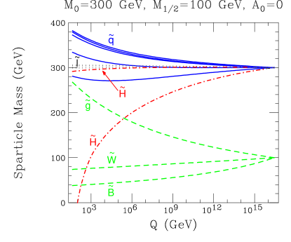
Figure 1: Evolution of masses in the SUGRA model, from Ref. Bagger95.

III Minimal SUGRA Model

The most general MSSM has more than 100 parameters. Many recent phenomenological studies have been based on a more restrictive model, the minimal supergravity (SUGRA) modelSUGRA . This is very similar to the Constrained MSSMCMSSM , although the latter adds some additional constraints. If SUSY breaking is communicated through gravity, then it is plausible that the SUSY breaking terms, like gravity, are universal at the GUT scale. In particular, if all the scalar masses are identical, then electroweak symmetry must be unbroken. It turns out that the Clebsch-Gordon coefficients are such that when the parameters are run from the GUT scale to the weak scale using the renormalization group equations, the large top Yukawa coupling drives the mass-squared of the Higgs negative, breaking electroweak symmetry but not color or charge. A example of this evolution is shown in Fig. 1. It is convenient to eliminate $B$ and $\mu^{2}$ in favor of $M_{Z}$ and $\tan\beta$. Then the minimal SUGRA model is characterized by just four parameters and the sign of $\mu$:

• $m_{0}$: the common squark, slepton, and Higgs mass at $M_{\rm GUT}$.

• $m_{1/2}$: the common gaugino mass at $M_{\rm GUT}$.

• $A_{0}$: the common trilinear coupling at $M_{\rm GUT}$.

• $\tan\beta=v_{1}/v_{2}$: the ratio of Higgs vacuum expectation values at $M_{Z}$.

• $\mathop{\rm sgn}\mu=\pm 1$.

It turns out that $A_{0}$ is not very important for phenomenology at the weak scale.

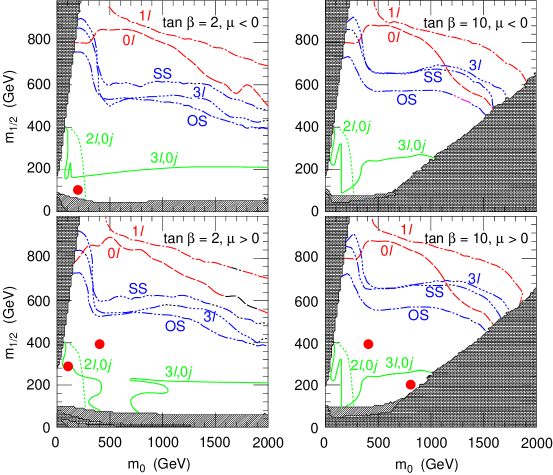
Figure 2: SUGRA discovery limits in the SUGRA model at the LHC with $10\,{\rm fb}^{-1}$ integrated luminosity. $0\ell$: $\hbox to0.0pt{\hbox to7.95831pt{\hfil/\hfil}\hss}E_{T}$ + jets + no leptons. $1\ell$: $\hbox to0.0pt{\hbox to7.95831pt{\hfil/\hfil}\hss}E_{T}$ + jets + one lepton. $OS$: Opposite sign dileptons. $SS$: same sign dileptons. $3\ell$: trileptons. $2\ell,0j$: dileptons with jet veto (from slepton production). $3\ell,0j$: trileptons with jet veto (from gaugino production). From Ref. BCPT2.

While the SUGRA model provides a much more tractable parameter space than the general MSSM, one should remember that it is only one possible model. It is possible that the assumption of universal masses is not correct. It is also possible that SUSY breaking is communicated at a much lower mass scale, as in gauge mediated modelsDine .

IV SUSY Signatures at LHC

The LHC is a $pp$ collider with an energy of $14\,{\rm TeV}$, enough to produce ${\tilde{g}}$ and ${\tilde{q}}$ pairs with $\mathrel{\hbox to0.0pt{\raise 2.20013pt\hbox{$<$}\hss}{\lower 2.20013pt\hbox{$\sim$}}}2\,{\rm TeV}$ even with $10\,{\rm fb}^{-1}$. These are typically produced with $p_{T}\sim M$, so they move slowly in the lab frame and their decay products are widely separated. If $R$ parity is conserved, they will decay into the LSP $\tilde{\chi}_{1}^{0}$ plus multiple jets and perhaps multiple leptons. A typical decay chain might be:

$${\tilde{g}} \to {\tilde{q}}_{L}+\bar{q}$$

$${\tilde{q}}_{L} \to {\tilde{\chi}}_{2}^{0}+q$$

$${\tilde{\chi}}_{2}^{0} \to {\tilde{\ell}}_{R}+\bar{\ell}$$

$${\tilde{\ell}}_{R} \to \tilde{\chi}_{1}^{0}+\ell$$

Such decay chains produce many possible signatures combining jets, leptons, and $\hbox to0.0pt{\hbox to7.95831pt{\hfil/\hfil}\hss}E_{T}$ from $\tilde{\chi}_{1}^{0}$ and $\nu$’s. For example, since the ${\tilde{g}}$ is self-conjugate, there are isolated same-sign dileptons $\ell^{\pm}\ell^{\pm}$.

The $5\sigma$ discovery limits at the LHC for $10\,{\rm fb}^{-1}$ integrated luminosity are shown in Figure 2. Note that the reach is $>2\,{\rm TeV}$ in the missing energy channels and $>1\,{\rm TeV}$ in the multi-lepton channels. Thus the LHC should find multiple signatures for SUSY with only $10\,{\rm fb}^{-1}$ if it exists at the weak scale.

V Precision Measurements at LHC

While it is easy to find signals for SUSY at LHC, there are two missing $\tilde{\chi}_{1}^{0}$’s in each event, making it difficult to reconstruct masses. However, it is possibleHPSSY to exploit the cascade decays characteristic of the MSSM to determine combinations of masses. The strategy is to start at the bottom of the decay chain and work up, partially reconstruct specific final states and relating precision measurements of endpoints of kinematic distributions to combinations of masses. A global fit to these combinations can then be used to determine the model parameters, at least in favorable cases. It would be better to make the global fit not just to such endpoints but to all distributions, but this is more difficult technically and perhaps premature at this stage.

What combinations of masses can be determined in this way depends on the decay modes and so requires study of specific SUSY models. The CERN LHC Program Committee (LHCC) chose five SUGRA points for detailed study by the ATLAS and CMS Collaborations. The parameters of these points and some representative masses are listed in Table 1. Point 3 is the “comparison point,” selected so that every existing or proposed accelerator can discover something. Point 5 was chosen to give the right cold dark matter for cosmology and so is perhaps the most realistic. Points 1 and 2 have gluino and squark masses of order $1\,{\rm TeV}$. Point 4 has the squarks much heavier than the gluinos. It is close to the boundary allowed by electroweak symmetry breaking (at least with ISAJET 7.22) and so has a relatively small $\mu$ and a large mixing between gauginos and Higgsinos. Studying these specific points has proved surprisingly usefulBartl96 ; HPSSY ; ATLASSUSY ; CMSSUSY .

Table 1: Parameters of the LHCC SUGRA points and some representative masses from ISAJET 7.22ISAJET .

Point	$m_{0}$	$m_{1/2}$	$A_{0}$	$\tan\beta$	$\mathop{\rm sgn}{\mu}$	$M_{\tilde{g}}$	$M_{\tilde{u}_{R}}$	$M_{\tilde{W}_{1}}$	$M_{\tilde{e}_{R}}$	$M_{h}$
	(GeV)	(GeV)	(GeV)			(GeV)	(GeV)	(GeV)	(GeV)	(GeV)
1	400	400	0	02.0	$+$	1004	925	325	430	111
2	400	400	0	10.0	$+$	1008	933	321	431	125
3	200	100	0	02.0	$-$	0298	313	096	207	068
4	800	200	0	10.0	$+$	0582	910	147	805	117
5	100	300	300	02.1	$+$	0767	664	232	157	104

VI Effective Mass

Gluinos and squarks are strongly produced at the LHC. But production cross sections fall rapidly with the produced mass, so it is important to find a variable that measures the produced mass for events with missing particles. A variable that works well for SUSY is the effective mass, defined as the sum of the missing energy and the $p_{T}$’s of the first four jets,

$$M_{\rm eff}=\hbox to0.0pt{\hbox to7.95831pt{\hfil/\hfil}\hss}E_{T}+p_{T,1}+p_{T,2}+p_{T,3}+p_{T,4}$$

Samples of signal and Standard Model background events were generated with ISAJETISAJET . To separate SUSY from the Standard Model background, events were selected with multiple jets plus missing energy:

• $\hbox to0.0pt{\hbox to7.95831pt{\hfil/\hfil}\hss}E_{T}>\max(100\,{\rm GeV},0.2M_{\rm eff})$;

• $\geq 4$ jets with $p_{T}>50\,{\rm GeV}$ and $p_{T,1}>100\,{\rm GeV}$;

• Transverse sphericity $S_{T}>0.2$;

• No $\mu$ or isolated $e$ with $p_{T}>20\,{\rm GeV}$, $\eta<2.5$.

Then the SUSY signal emerges from the Standard Model background for large $M_{\rm eff}$, as can be seen from Figure 3. The signal cross section is of order $1\,{\rm pb}$ in the region where it dominates, so it could be discovered in about one month at $10^{32}\,{\rm cm^{-2}s^{-1}}$. (Of course, it would take much longer than this to understand the detectors.)

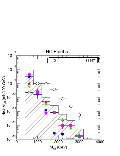
Figure 3: $M_{\rm eff}$ distributions after cuts. Open circles: SUSY signal. Solid circles: $t\bar{t}$. Upward triangles: $W$ + jets. Downward triangles: $Z$ + jets. Squares: QCD jets. Shaded histogram: Sum of Standard Model backgrounds. From Ref HPSSY.

The value of $M_{\rm eff}$ at which the signal emerges from the background scales with the SUSY mass scale. To test this, 100 random SUGRA models were generated, and the peak of the $M_{\rm eff}$ signal was compared with the SUSY mass scale, defined by

$$M_{\rm SUSY}=\min(M_{\tilde{g}},M_{\tilde{u}})$$

The scatter plot, shown in Fig. 4, shows a good correlation between the peak and the SUSY mass scale, allowing one to determine the SUSY mass scale to about 10%.

Figure 4: Scatter plot of signal peak in $M_{\rm eff}$ vs. ${M_{\rm SUSY}}$ defined in text. From Ref. HPSSY.

VII Reconstruction of Specific Final States

The precision measurements of specific combinations of masses are based on the partial reconstruction of the corresponding final states. For each case, SUSY and Standard Model background event samples were generated with ISAJETISAJET or PYTHIAPYTHIA , a simple particle-level detector simulation incorporating resolutions characteristic of ATLAS and CMS was made, and analysis cuts as described below were applied.

VII.1 Measurement of $M({\tilde{\chi}}_{2}^{0})-M(\tilde{\chi}_{1}^{0})$

The prototype of all the precision measurements is based on the decay ${\tilde{\chi}}_{2}^{0}\to\tilde{\chi}_{1}^{0}\ell^{+}\ell^{-}$ at Point 3. Point 3 has unusual branching ratios:

$$B({\tilde{g}}\to{\tilde{b}}_{1}\bar{b}+{\rm h.c.}) = 89\%$$

$$B({\tilde{b}}_{1}\to{\tilde{\chi}}_{2}^{0}b) = 86\%$$

$$B({\tilde{\chi}}_{2}^{0}\to\tilde{\chi}_{1}^{0}\ell^{+}\ell^{-}) = 2\times 17\%$$

The dominant decay of ${\tilde{g}}\to{\tilde{b}}_{1}\bar{b}$ arises because the ${\tilde{b}}_{1}$ is lighter than the ${\tilde{g}}$ but the other squarks are heavier. Events were selected to have two leptons and two $b$ jets:

• $\ell^{+}\ell^{-}$ pair with $p_{T,\ell}>10\,{\rm GeV}$, $\eta<2.5$.

• $\geq 2$ jets tagged as $b$ quarks with $p_{T}>15\,{\rm GeV}$ and $\eta<2$.

• No $\hbox to0.0pt{\hbox to7.95831pt{\hfil/\hfil}\hss}E_{T}$ cut was used.

All distributions shown include a 60% tagging efficiency for $b$’s and 90% efficiency for leptons within the kinematic cuts given above.

The result of this analysis is a spectacular edge at $M({\tilde{\chi}}_{2}^{0})-M(\tilde{\chi}_{1}^{0})$ endpoint with almost no Standard Model background, as can be seen in Figure 5. Most of the SUSY background comes from two ${\tilde{\chi}}_{1}^{\pm}$ decays and can be removed by plotting the distribution for

$$e^{+}e^{-}+\mu^{+}\mu^{-}-2e^{\pm}\mu^{\mp}$$

This analysis clearly would have huge statistics and would be much easier than measuring $M_{W}$ at Tevatron. Given the current $M_{W}$ results, it seems conservative to estimate an error

$$\Delta(M({\tilde{\chi}}_{2}^{0})-M(\tilde{\chi}_{1}^{0}))=50\,{\rm MeV}$$

for $10\,{\rm fb}^{-1}$.

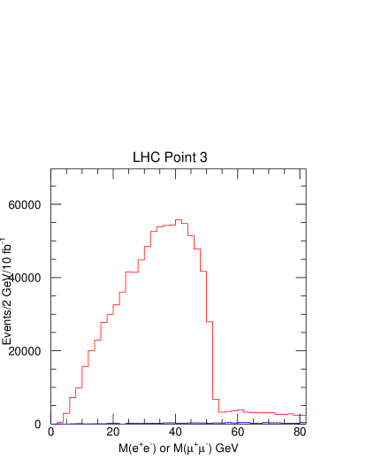
Figure 5: $\ell^{+}\ell^{-}$ distribution for SUSY events at Point 3 (histogram) and for Standard Model background (shaded) after cuts described in the text. From Ref .HPSSY.

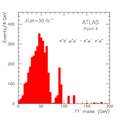
Figure 6: $\ell^{+}\ell^{-}$ distribution for SUSY events at Point 4. From Ref .Fabiola.

Point 3 is perhaps unusually easy, but there is a similar edge at Point 4 plus $Z$ peak from heavier gauginos, as can be seen from Figure 6. The estimated error in this case is $\pm 1\,{\rm GeV}$.

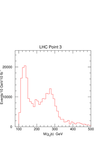
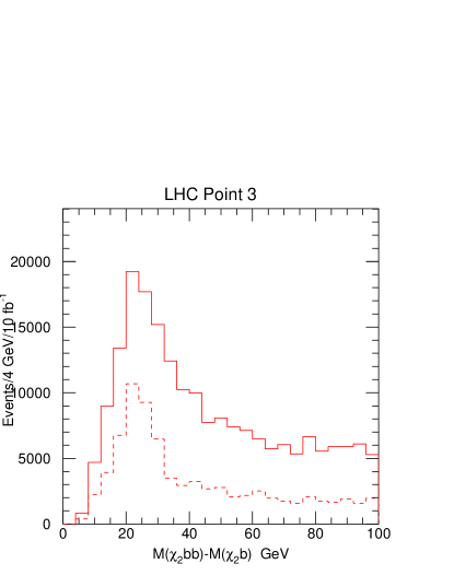
Figure 7: Projections of the gluino-sbottom mass scatter plot. From HPSSY.

VII.2 ${\tilde{g}}$ and ${\tilde{b}}_{1}$ Reconstruction

The next step at Point 3 is to combine an $\ell^{+}\ell^{-}$ pair near the edge with jets to determine the ${\tilde{b}}_{1}$ and ${\tilde{g}}$ masses. Events were selected with

• $\geq 2$ jets tagged as $b$ jets with $p_{T}>15\,{\rm GeV}$, $\eta<2$;

• $\ell^{+}\ell^{-}$ pair with $45<M(\ell\ell)<55\,{\rm GeV}$.

For an $\ell^{+}\ell^{-}$ pair near the endpoint, the $\tilde{\chi}_{1}^{0}$ must be soft in the ${\tilde{\chi}}_{2}^{0}$ rest frame, so that

$$\vec{p}({\tilde{\chi}}_{2}^{0})\approx\left({1+{M(\tilde{\chi}_{1}^{0})\over M(\ell\ell)}}\right)\vec{p}(\ell\ell)$$

where $M(\tilde{\chi}_{1}^{0})$ must be determined from a global fit. The approximately reconstructed ${\tilde{\chi}}_{2}^{0}$ was combined with one of masses coming from combining the ${\tilde{\chi}}_{2}^{0}$ with one $b$ to make $M({\tilde{b}}_{1})$ and with a second $b$ to make $M({\tilde{g}})$ using the correct $\tilde{\chi}_{1}^{0}$ mass. The resulting projections, shown in Figure 7, display good resolution on the mass difference between the ${\tilde{g}}$ and the ${\tilde{b}}_{1}$ masses — just like for $D^{*}\to D\pi$. By varying the assumed $\tilde{\chi}_{1}^{0}$ mass, one finds

$$\Delta M({\tilde{b}}_{1})=\pm 1.5\Delta M(\tilde{\chi}_{1}^{0})\pm 3\,{\rm GeV}$$

$$\Delta\left({M({\tilde{g}})-M({\tilde{b}}_{1})}\right)=\pm 2\,{\rm GeV}$$

VII.3 Reconstruction of $h\to b\bar{b}$

For Point 5, the decay ${\tilde{\chi}}_{2}^{0}\to\tilde{\chi}_{1}^{0}h$ is kinematically allowed and has a branching ratio of 64%. Events were selected with

• $\geq 4$ jets with $p_{T}>50\,{\rm GeV}$, $p_{T,1}>100\,{\rm GeV}$;

• Transverse sphericity $S_{T}>0.2$;

• $M_{\rm eff}=\hbox to0.0pt{\hbox to7.95831pt{\hfil/\hfil}\hss}E_{T}+\sum_{i=1}^{4}\,p_{T,i}>800\,{\rm GeV}$;

• $\hbox to0.0pt{\hbox to7.95831pt{\hfil/\hfil}\hss}E_{T}>\max(100\,{\rm GeV},0.2M_{\rm eff})$.

and the $b\bar{b}$ mass was plotted for all pairs of $b$ jets with $p_{T,b}>25\,{\rm GeV}$ and $\eta_{b}<2$. A correction factor was applied to the measured $b$ jet energies to account for neutrinos and energy loss out of the cone, and a 60% $b$-tagging efficiency was assumed. The resulting distribution, Figure 8, has a peak at the Higgs mass with a substantial SUSY background but very little Standard Model background. This signal is much easier than $h\to\gamma\gamma$ and would be the discovery mode for the Higgs at this point.

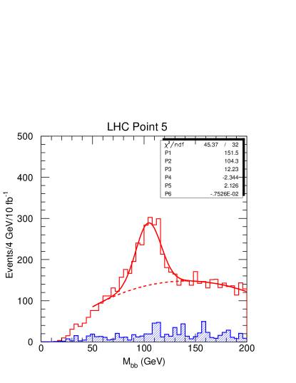
Figure 8: $M(b\bar{b})$ for pairs of $b$ jets for the Point 5 signal (open histogram) and for the sum of all backgrounds (shaded histogram). The smooth curve is a Gaussian plus quadratic fit to the signal. The light Higgs mass is $104.15\,{\rm GeV}$.

The $h\to b\bar{b}$ candidates can be used to reconstruct the decay chain

$${\tilde{g}}+{\tilde{g}}\to{\tilde{q}}_{L}q+{\tilde{q}}_{R}q$$

$${\tilde{q}}_{L}\to{\tilde{\chi}}_{2}^{0}q\to\tilde{\chi}_{1}^{0}hq,\qquad{\tilde{q}}_{R}\to\tilde{\chi}_{1}^{0}q$$

To select these events exactly two additional jets with $p_{T}>75\,{\rm GeV}$ were required. Then since one of the two $qb\bar{b}$ combinations comes from the squark decay, the smaller of them must have an endpoint at a function of the squark mass and the other masses in the problem. The squark mass can be measured to about $40\,{\rm GeV}$ in this way.

VII.4 $\ell^{+}\ell^{-}$ Again

Consider dileptons for Point 5. The mass distribution after the by now standard cuts shows a dramatic edge at about $109\,{\rm GeV}$. Since this decay must compete with the two-body decay ${\tilde{\chi}}_{2}^{0}\to\tilde{\chi}_{1}^{0}h$, it cannot be a direct three-body decay ${\tilde{\chi}}_{2}^{0}\to\tilde{\chi}_{1}^{0}\ell^{+}\ell^{-}$. In fact it comes from two sequential two-body decays, ${\tilde{\chi}}_{2}^{0}\to{\tilde{\ell}}^{\pm}\ell^{\mp}\to\tilde{\chi}_{1}^{0}\ell^{\pm}\ell^{\mp}$, and the edge determines

$$M_{\rm max}(\ell\ell)=M({\tilde{\chi}}_{2}^{0})\sqrt{1-{M_{\tilde{\ell}}^{2}\over M_{\tilde{\chi}_{2}^{0}}^{2}}}\sqrt{1-{M_{\tilde{\chi}_{1}^{0}}^{2}\over M_{\tilde{\ell}}^{2}}}$$

to about $1\,{\rm GeV}$. One should do a complete fit to the Higgs and dilepton events to extract the maximum information on all the masses. This has not yet been done. The variable most sensitive to the slepton mass is $p_{T,2}/p_{T,1}$. This distribution was compared for two different values of $m_{0}$, from which it seems that the slepton mass can be estimated to $\Delta M({\tilde{\ell}}_{R})\sim 3\,{\rm GeV}$.

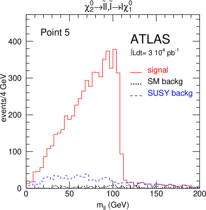
Figure 9: $M_{\ell\ell}$ for the Point 5 signal (open histogram) and the sum of all backgrounds (shaded histogram). From Ref. Polesello.

VII.5 Measurement of $M({\tilde{g}})-M({\tilde{\chi}}_{2}^{0}),M({\tilde{\chi}}_{1}^{\pm})$

Gluinos dominate at Point 4 since $m_{0}$ is large. This means that there is a lot of combinatorial background from the many jets in the final state. The strategy of this analysisATLASSUSY ; Fabiola is to use trilepton events to select the process

$${\tilde{g}}+{\tilde{g}}\to{\tilde{\chi}}_{2}^{0}q\bar{q}+{\tilde{\chi}}_{1}^{\pm}q\bar{q}$$

Then the dijet mass distributions for the right jet pairing have a common endpoint since $M({\tilde{\chi}}_{2}^{0})\approx M({\tilde{\chi}}_{1}^{\pm})$.

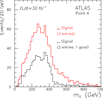
Figure 10: Dijet mass distributions for Point 4 after cuts. The dashed curve shows only the right pairing based on generator information. From Ref. Fabiola.

Events were selected by requiring three leptons and four jets:

• 3 isolated $\ell$: $p_{T}>20$, 10, $10\,{\rm GeV}$, $|\eta|<2.5$

• One opposite-sign, same-flavor lepton pair with $M_{\ell\ell}<72\,{\rm GeV}$.

• 4 jets; $p_{T}>150$, 120, 70, $40\,{\rm GeV}$, $|\eta|<3.2$.

• No additional jets with $p_{T}>40\,{\rm GeV}$ and $|\eta|<5$ to minimize combinatorics.

No $\hbox to0.0pt{\hbox to7.95831pt{\hfil/\hfil}\hss}E_{T}$ cut was used. With these cuts there are 250 signal events, 30 ${\tilde{g}}{\tilde{q}}$ background events, and 18 other SUSY and Standard Model background events for $30\,{\rm fb}^{-1}$. The pairing between the two highest and the two lowest $p_{T}$ jets is usually wrong and so was eliminated. The dijet mass distribution for the other pairings is shown in Figure 10. There is an endpoint at about the right point.

VIII Fitting SUGRA Parameters

The precision measurements described here are only a fraction of those in Refs. HPSSY, Fabiola, and Polesello. Ideally one should combine these measurements with a large number of other ones and do a global fit, but this would require generating many signal signal event samples. Instead a much simpler procedure has been adopted. SUGRA parameters were generated at random, the mass spectrum for each SUGRA point was calculated, and these were compared with the precision measurements and their estimated errors.

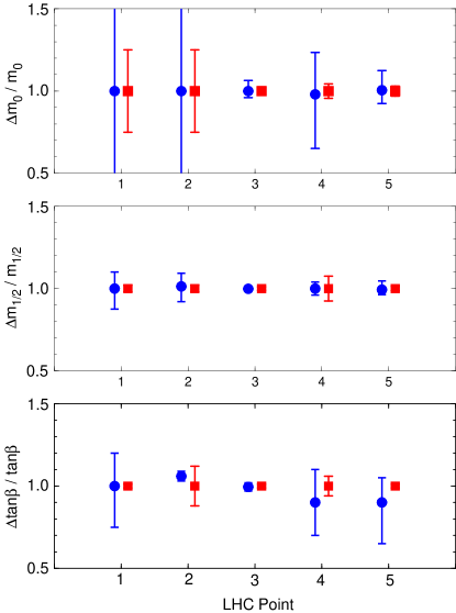
Figure 11: Errors from global fits to the SUGRA parameters. Circles: Fit I. Squares: Ultimate Fit II.

Two such fits have been made. Fit IHPSSY uses only the measurements developed in Ref. HPSSY. It assumes that the Higgs mass can be related to the SUGRA parameters with an error $\Delta M_{h}=3\,{\rm GeV}$, about the current theoretical error. It bases the statistical errors on $10\,{\rm fb}^{-1}$. Fit IIFroid adds some additional precision measurements developed after Ref. HPSSY. It adds some other data, e.g., from changing the squark masses at Points 1 and 2 and seeing the effect of this on the mean $p_{T}$ of the hardest jet. This is not fully justified, but it is a plausible way of estimating the improvement from fitting some of the kinematic distributions as well as the precision measurements. The ultimate version of Fit II also assumes a theoretical error on the Higgs mass less than the expected experimental error from $h\to\gamma\gamma$, $\Delta M_{h}=0.2\,{\rm GeV}$ and scales the statistical errors to $300\,{\rm fb}^{-1}$.

Both fits scanned the SUGRA parameter space and determined the 68% confidence interval for each parameter. The results are summarized in Figure 11. No disconnected solutions were found. In particular, $\mathop{\rm sgn}\mu$ was correctly determined, although this required including additional information in the fit in some cases. The gluino and squark masses are insensitive to $m_{0}$ at Points 1 and 2, and there is no information available on the slepton masses, accounting for the larger errors on $m_{0}$ at these points. Finally, $A_{0}$ is poorly constrained in all cases, even for the ultimate version of Fit II. It is possible to determine the weak scale parameters $A_{t}$ and $A_{b}$, but these are insensitive to $A_{0}$.

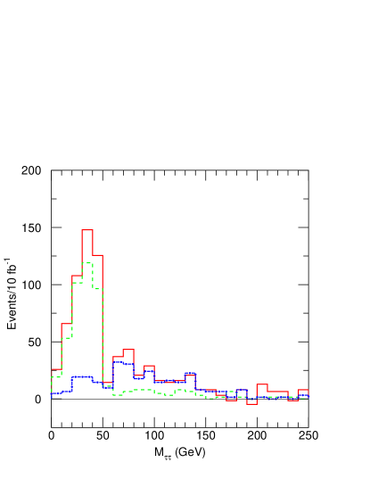
Figure 12: Solid: Visible $\tau\tau$ mass distribution for 3-prong $\tau$ decays. Dashed: Contribution from ${\tilde{\chi}}_{2}^{0}\to{\tilde{\tau}}\tau$. Dash-dotted: Contribution from higher mass gauginos.

IX $\tau$ Modes at Large $\tan\beta$

The five LHCC points do not exhaust the possibilities of even the minimal SUGRA model. For example, the ${\tilde{\tau}}_{1}$ is light for large $\tan\beta$, so $\tau$ decays can be dominant. Consider the SUGRA point $m_{0}=m_{1/2}=200\,{\rm GeV}$, $A_{0}=0$, $\tan\beta=45$, $\mu<0$. Then

$$B({\tilde{\chi}}_{2}^{0}\to{\tilde{\tau}}_{1}^{\pm}\tau^{\mp})\approx B({\tilde{\chi}}_{1}^{\pm}\to{\tilde{\tau}}_{1}^{\pm}\nu_{\tau})\approx 100\%$$

Discovery of the SUSY signal is still straightforward, but none of the precision measurements discussed above are applicable.

One possible approach is to require two 3-prong hadronic $\tau$’s to maximize the visible $\tau\tau$ mass and hence its sensitivity to the endpoint analogous to that discussed in Section VII.D. The difference of $\tau^{+}\tau^{-}$ and $\tau^{\pm}\tau^{\pm}$ is used to eliminate the contribution from two ${\tilde{\chi}}_{1}^{\pm}$ decays. The resulting distribution is shown in Figure 12. There is clearly an endpoint visible from the contribution of ${\tilde{\chi}}_{2}^{0}\to{\tilde{\tau}}\tau$ plus a contribution from heavier gauginos. Signatures like this require more study both for the Tevatron and for the LHC.

X Outlook for Lepton Colliders

If SUSY exists at the electroweak scale, it should be straightforward to find signals for it at the LHC. It is possible in many cases to make precision measurements, and if the SUSY model is relatively simple, these can be used to determine its parameters.

The LHC will mainly produce gluinos and squarks. In SUGRA these tend to decay mainly into the lighter gauginos; the heavier ones are dominantly Higgsino and so are suppressed both by their masses and by their couplings. The direct production of sleptons and sneutrinos is also very small, although they can be produced as decay products of the light gauginos if they are light enough. Finally, the heavy Higgs bosons have small production cross sections, and their dominant decay modes have large backgrounds. One should not underestimate the ingenuity of experimentalists with real data, but it seems likely that the LHC will not be able to study the entire SUSY spectrum.

A Next Lepton Collider with $\sqrt{s}\sim 500\,{\rm GeV}$ should be able to detect any SUSY particles except the $\tilde{\chi}_{1}^{0}$ that are kinematically accessible. Sleptons probably represent the best opportunity to make significant progress beyond what has been learned from the LHC. One of the attractive features of the SUGRA model is that the $\tilde{\chi}_{1}^{0}$ is a good dark matter candidate, and the abundance of cold dark matter favors light sleptonsCDM . A lepton collider provides an important additional constraint that the slepton pairs are produced with known energy, and this allows precise measurements to be madeTFMYO ; NFT . But if more than one slepton is being produced, the spectrum can be quite complex, so high luminosity (as well as enough energy) may be essential.

References

- (1) For general reviews of SUSY, see H.P. Nilles, Phys. Rep. 111, 1 (1984); H.E. Haber and G.L. Kane, Phys. Rep. 117, 75 (1985).
- (2) P. Janot, Int. Euro. Conf. on High Energy Physics (Jerusalem, 1997), http://www.cern.ch/hep97/pl17.htm.
- (3) M. Carena, P. Zerwas, et al., hep-ph/9602250, CERN-96-01 (1996).
- (4) G.L. Kane, C. Kolda, and J.D. Wells, Phys. Rev. Lett. 70, 2686 (1993).
- (5) P.Q. Hung and M. Sher, Phys. Lett. B374, 138 (1996).
- (6) H. Baer, H. Murayama, X. Tata, et al., FSU-HEP-950401, hep-ph/9503479 (1995).
- (7) H. Baer, C-H Chen, F.E. Paige, and X. Tata, Phys. Rev. D52, 2746 (1995).
- (8) ATLAS Collaboration, Technical Proposal, LHCC/P2 (1994).
- (9) CMS Collaboration, Technical Proposal, LHCC/P1 (1994).
- (10) G.W. Anderson and D.J. Castano, Phys. Lett. B347, 300 (1995).
- (11) H. Baer, C-H Chen, F.E. Paige, and X. Tata, Phys. Rev. D53, 6241 (1996).
- (12) U. Amaldi, A. Bohm, L.S. Durkin, P. Langacker, A.K. Mann, W.J. Marciano, A. Sirlin, H.H. Williams, Phys. Rev. D36, 1385 (1987).
- (13) L. Alvarez-Gaume, J. Polchinski and M.B. Wise, Nucl. Phys. B221, 495 (1983); L. Ibañez, Phys. Lett. 118B, 73 (1982); J.Ellis, D.V. Nanopolous and K. Tamvakis, Phys. Lett. 121B, 123 (1983); K. Inoue et al. Prog. Theor. Phys. 68, 927 (1982); A.H. Chamseddine, R. Arnowitt, and P. Nath, Phys. Rev. Lett., 49, 970 (1982).
- (14) G.L. Kane, C. Kolda, L. Roszkowski, and J.D. Wells, Phys. Rev. D49, 6173 (1994).
- (15) M. Dine, A.E. Nelson, and Y. Shirman, Phys. Rev. D51, 1362 (1995).
- (16) J. Bagger, hep-ph/9508392 (1995).
- (17) A. Bartl, J. Soderqvist, et al., in 1996 DPF/DPB Summer Study on New Directions for High-Energy Physics (Snowmass 96).
- (18) I. Hinchliffe, F.E. Paige, M.D. Shapiro, J. Söderqvist, and W. Yao, Phys. Rev. D55, 5520 (1997).
- (19) ATLAS Collaboration, SUSY Presentations to the LHCC (October, 1996).
- (20) CMS Collaboration, SUSY Presentations to the LHCC (October, 1996).
- (21) H. Baer, F. Paige, S. Protopopescu and X. Tata; in Physics at Current Accelerators and Supercolliders, ed. J. Hewett, A. White and D. Zeppenfeld, (Argonne National Laboratory, 1993).
- (22) T. Sjostrand, LU-TP-95-20, hep-ph/9508391 (1995); S. Mrenna, Comput. Phys. Commun. 101, 232 (1997).
- (23) F. Gianotti, ATLAS Internal Note PHYS-No-110 (1997).
- (24) G. Polesello, L. Poggioli, E. Richter-Was, and J. Soderqvist, ATLAS Internal Note PHYS-No-111 (1997).
- (25) D. Froidevaux, http://atlasinfo.cern.ch/Atlas/GROUPS/PHYSICS/SUSY/lhcc/daniel.ps.Z.
- (26) J. Ellis and L. Roszkowski Phys. Lett. B283, 252, (1992); H. Baer and M. Brhlik, Phys. Rev. D53, 597 (1996).
- (27) T. Tsukamoto, K. Fujii, H. Murayama, M. Yamaguchi, and Y. Okada, Phys. Rev. D51, 3153, (1995).
- (28) M.M. Nojiri, K. Fujii, and T. Tsukamoto Phys. Rev. D54, 6756 (1996).