Methods in the LO Evolution of Nondiagonal Parton Distributions: The DGLAP Case
Abstract
In this paper, we discuss the algorithms used in the LO evolution program
for nondiagonal parton distributions in the DGLAP region and discuss the
stability of the code.
Furthermore, we demonstrate that we can reproduce the case of the LO diagonal
evolution within of the original code as developed by the
CTEQ-collaboration.
PACS: 12.38.Bx, 13.85.Fb, 13.85.Ni
Keywords: Deeply Virtual Compton Scattering, Nondiagonal distributions,
Evolution
I Introduction
Due to the recent availability of exclusive hard diffraction data at HERA, there has been a great interest in the study of generalized parton distributions also known as nondiagonal, off-forward or non-forward parton distributions occurring in these reactions (see Ref. [1, 2, 3, 4, 5, 6, 7, 8, 9, 10, 11]). These parton distributions are different from the usual, diagonal distributions found in e.g. inclusive DIS since one has a finite momentum transfer to the proton due to the exclusive nature of the reactions. In this paper we give an exposition of the algorithms used to numerically solve the generalized GLAP-evolution equations. The main part of the evolution program was taken over from the CTEQ package for the diagonal parton distributions from inclusive reactions. At this point in time the evolution kernels for generalized parton distributions are known only to leading order in and thus our analysis will be a leading order one.
The paper is organized in the following way. In Sec. II we will quickly review the formal expressions for the parton distributions and the evolution equations together with the explicit expressions for the kernels and a first comment on the arising numerical problems. In Sec. III we will explain the difference of our algorithms to the ones used in the original CTEQ package and then give a detailed account of how we implemented our algorithms. In Sec. IV we demonstrate the stability of our code and show that we reproduce the case of the usual or diagonal parton distributions within for a vanishing asymmetry factor. Sec. V contains concluding remarks.
II Review of Nondiagonal Parton Distributions, Evolution Equations and Kernels
A Nondiagonal Parton Distributions
Generalized or, from now on nondiagonal parton distributions, occur for example in exclusive, hard diffractive or meson production and alternatively in deeply virtual Compton scattering (DVCS), where a real photon is produced. As mentioned in Sec. I since one imposes the condition of exclusiveness on top of the diffraction condition, one has a kinematic situation in which there is a non-zero momentum transfer onto the target proton as evidenced by the lowest order “handbag” diagram of DVCS in Fig. 1. The picture serves to only introduce the kinematic notations used throughout the text and nothing more. For more on DVCS see for example Ref. [6, 7, 12, 13, 14, 15, 16, 17, 18, 19, 20].

The nondiagonal quark and gluon distributions have the following formal definition as matrix elements of bilocal, path-ordered and renormalized quark and gluon operators sandwiched between different momentum states of the proton as in the factorization theorems for exclusive vector meson production [4] and DVCS [7, 19, 20]:
| (1) | |||
| (2) |
with where the asymmetry or nondiagonality parameter is usually in, for example, DVCS or exclusive vector meson production however not in diffractive di-muon production.
B The GLAP-Evolution Equations for Nondiagonal Parton Distributions
The GLAP-evolution equations follow from the usual renormalization group invariance of the factorization formula and lead to the following evolution equations for the singlet(S) and non-singlet(NS) case [5, 6, 7]:
| (3) | |||
| (4) | |||
| (5) |
Note that , and the kernels to leading order[21] are given by [5, 6, 7]:
| (6) | |||||
| (7) | |||||
| (8) | |||||
| (10) | |||||
With our definitions, we obtain for the diagonal limit, i.e. , , and where and are the usual parton densities.
A word concerning the above employed regularization prescription which is the usual + - prescription in the first integral below and a generalized + - prescription for the second integral, is in order, since these prescriptions have direct implications on the numerical treatment of the integrals involved. In convoluting the above kernels, after appropriate scaling of and with , with a nondiagonal parton density, one has to replace and in the regularization integrals with and . This leads to the following regularization prescription as employed in our modified version of the CTEQ package and in agreement with Ref. [7]:
| (11) | |||||
| (13) | |||||
Eq. 13 and a closer inspection of Eq. 10 reveals that if one were to integrate each term by itself one would encounter infinities in all the expressions at both the lower bound of integration if and in taking the limit . Although Eq. 10 is completely analytical, it will cause numerical problems since the cancellations of the infinite terms can only be done in the analytical expressions. This is in contrast to the diagonal case where such problems are absent. The integration over is identical to the diagonal case and hence has already been dealt with in the original CTEQ-code.
III Differences between the CTEQ and our Algorithms
Let us point out in the beginning that our code is to the original CTEQ-code (for a detailed account of this code see Ref. [22]). We only modified the subroutines NSRHSM, NSRHSP and SNRHS within the subroutine EVOLVE and added the subroutines NEWARRAY and NINTEGR. These routines are only dealing with the convolution integrals but not with, for example, the -integration or any other part of the CTEQ-code which remains unchanged. This is due to the fact that the main difference between the diagonal and nondiagonal evolution stems from the different kernels which only influence the convolution integration and nothing else.
In order to make the simple changes in the existing routines more obvious we will first deal with the new subroutines.
A NEWARRAY and NINTEGR
Due to the increased complexity of the convolution integrals as compared to the diagonal case as pointed out in Sec. II B, we were forced to slightly change the very elegant and fast integration routines employed in the original CTEQ-code. The basic idea, very close to the one in the CTEQ-code, is the following: Within the CTEQ package, the parton distributions are given on a dynamical - and -grid of variable size where the convolution of the kernels with the initial distribution is performed on the -grid. Due to the possibility of singular behavior of the integrands, we perform the convolution integrals by first splitting up the region of integration according to the number of grid points in , analytically integrating between two grid points and where runs from to the specified number of points in and then adding up the contributions from the small intervals as exemplified in the following equation:
| (14) |
where is the product of the initial distribution for each evolution step and an evolution kernel with , . We can do the integration analytically between two neighboring grid points by approximating the distribution function through a second order polynomial , using the fact that we know the function on the grid points and and can thus compute the coefficients a,b,c of the polynomial in the following way, given the function is well behaved and the neighboring grid points are close together [23]:
| (15) | |||||
| (16) | |||||
| (17) |
which yields a matrix relating the coefficients of the polynomial to the values of the distribution functions at and . Inverting this matrix in the usual way one obtains a matrix relating the values of the distribution function to the coefficients making it possible to compute them just from the knowledge of the different values and the value of the distribution function at those values. This calculation is implemented in NEWARRAY where the initial distribution is handed to the subroutine and the coefficient array is then returned. The coefficient array in which the values of the coefficients for the integration are stored, has times the size of the user-specified number of points in since we have coefficients for each bin in . We treat the last integration between the points and again by approximating the distribution in this last bin through a second order polynomial. However, for this last bin, the coefficients are computed using the last three values in and of the distribution at those points, since the point which would be required according to the above prescription for calculating the coefficients, does not exist.
After having regrouped the terms appearing in the convolution integral in such a way that all the necessary cancellations of large terms occur within the analytic expression for the integral and not between different parts of the convolution integral, the integration of the different terms is performed in the new subroutine NINTEGR with the aid of the coefficient array from NEWARRAY. As mentioned above the convolution integral from to is split up into several intervals in which the integration is carried out analytically. To give an example of this procedure we consider the convolution integral of with the parton distribution :
| (18) |
suppressing presently irrelevant factors in front of the integral. The two parts in Eq. 18 are calculated in different parts of NINTEGR and then put together in either NSRHSM, NSRHSP or SNRHS. In NINTEGR the integrals are split up according to Eq. 14 and then analytically evaluated in the different -bins [24]. If the dependence of the integrand on is only of a multiplicative nature it is enough to compute the integral for each bin once. To get the value of convolution integral for a term with such a [25] dependence, it is enough to store the result of the integration in the bin from to in the output array for this term at the position [26], add to this result the value of the integral in the bin from to and store it at the position and so forth. In this manner one only has to calculate integrals, however if the integrand has a more complicated dependence on like one needs to compute integrals. For example in order to find the integration value for the bin with one needs only one integral but at we have to redo our integral for the bin since plus we need to add the contribution from the bin to get the correct answer for the output array at position and so forth. This need for additional evaluations of integrals slows the program down but in the end it turns out to be only about a factor of slower ( as tested on a SPARC 10 ) than the original CTEQ-code which is speed optimized. The integral with the regular + - prescription is evaluated using the routine HINTEG from the original CTEQ-code whereas the generalized + - prescription is evaluated according to the methods described above due to its nontrivial dependence on and .
The case and , are implemented in NINTEGR in the same way as above but separately from each other and from the more general case. For the form of the integrands simplify in such a way that one can use the integration routines INTEGR and HINTEG from the original CTEQ-code. In the case of the analytic expressions obtained for the above general case are expanded to first order in and then the same methods as above for evaluating the integrals are applied. The last case also allows us to go to the diagonal case by setting without using the integration routines from the original CTEQ-code giving us a valuable tool to compare our code to the original one.
B Modifications in NSRHSM, NSRHSP and SNRHS
The modification in the already existing routines NSRHSM, NSRHSP and SNRHS of the original CTEQ package are rather trivial. The most notable difference is that the subroutine NEWARRAY is called every time either of the three subroutines is called since the distribution function handed down on an array changes with every call of NSRHSM, NSRHSP and SNRHS. In NSRHSM and NSRHSP, NEWARRAY is only called once since one is only dealing with the non-singlet part containing no gluons, whereas in SNRHS the subroutine for the singlet case, one needs a coefficient array for both the quark and the gluon. Besides this change, the calls for INTEGR are replaced by NINTEGR according to how the convolution integral has been regrouped as explained in Sec. III A. The different regrouped expressions are then added, after integration for different -values, to obtain the final answer in an output array which is handed back to the subroutine EVOLVE. The method is the same as in the original CTEQ-code but the terms themselves have changed of course.
IV Code Analysis
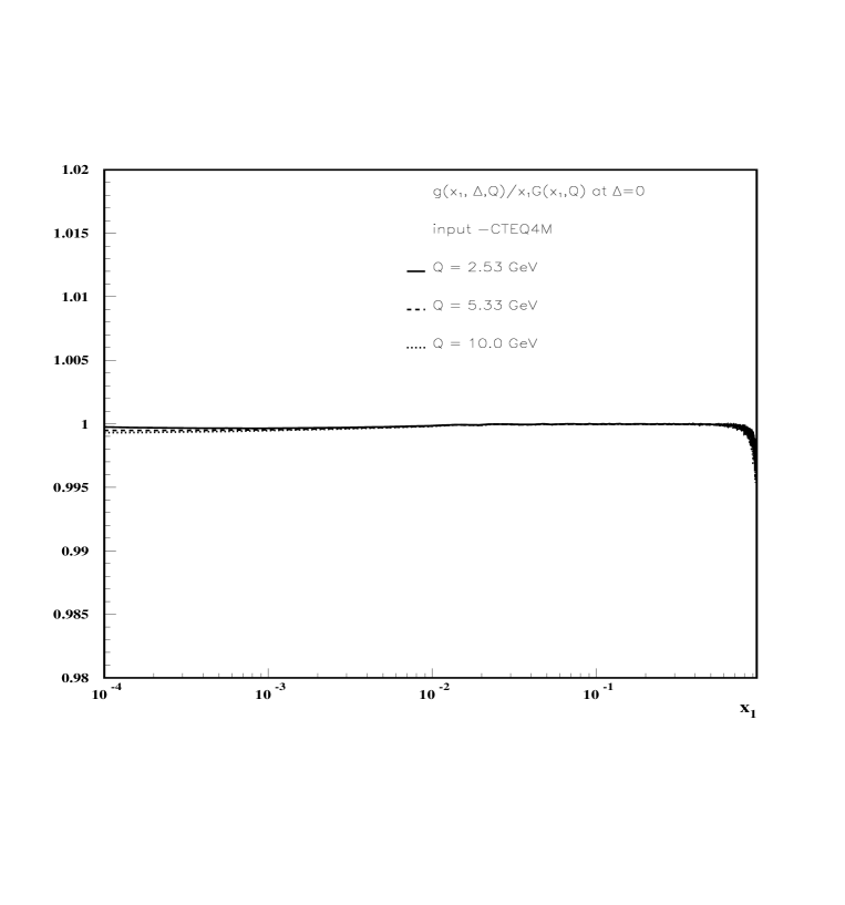
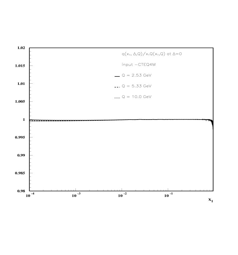
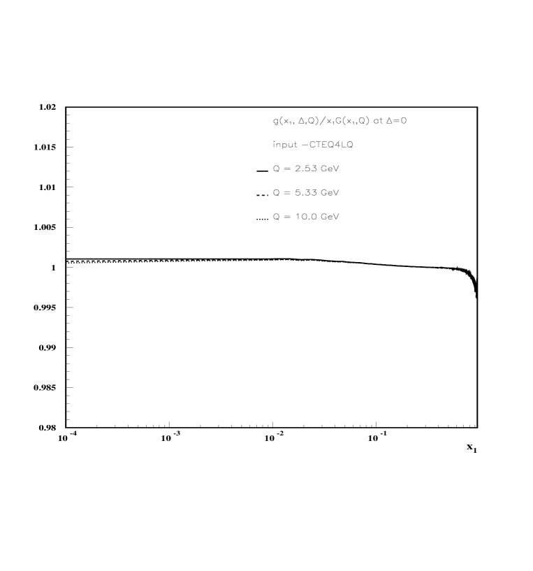
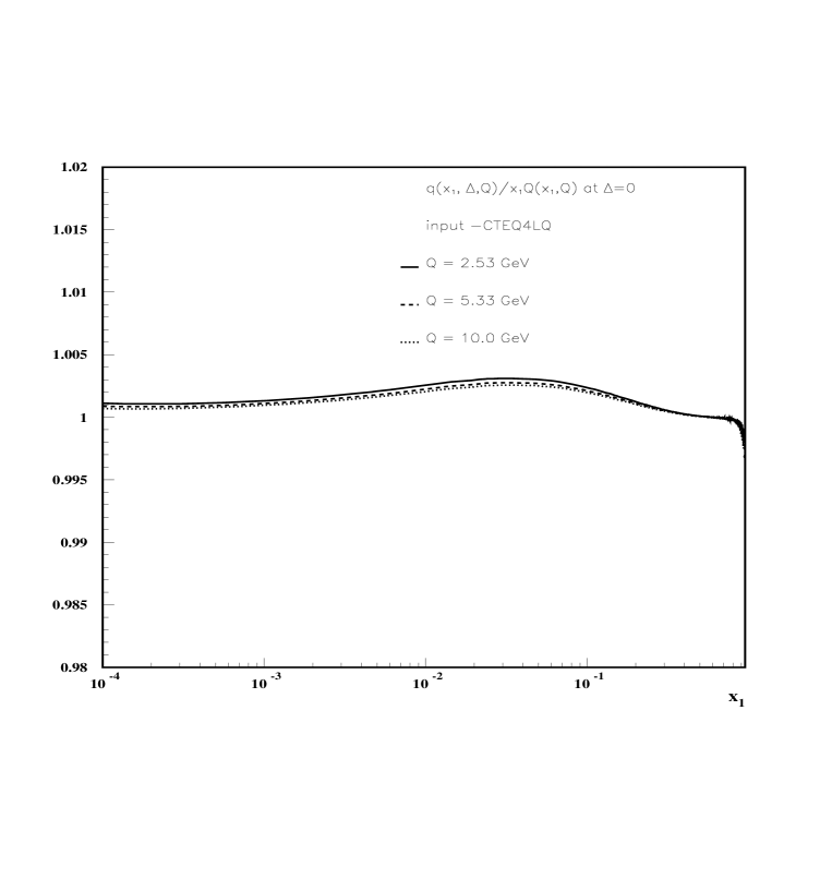
As a first step we tested the stability and speed of convergence of the code and found that by doubling the number of points in the -grid, which is only relevant for the convolution integral, from to the result of our calculation changed by less than , hence we can assume that our code converges rather rapidly. We also found the code to be stable down to an beyond which we did not test. Furthermore we can reproduce the result of the original CTEQ-code, i.e. the diagonal case in LO within giving us confidence that our code works well since the analytic expressions for the diagonal case are the expansions of the general case of non vanishing asymmetry up to, but not including, .
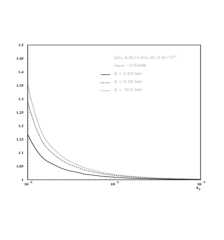
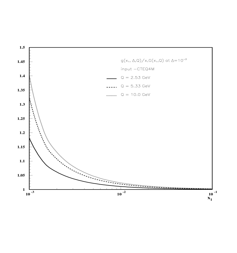
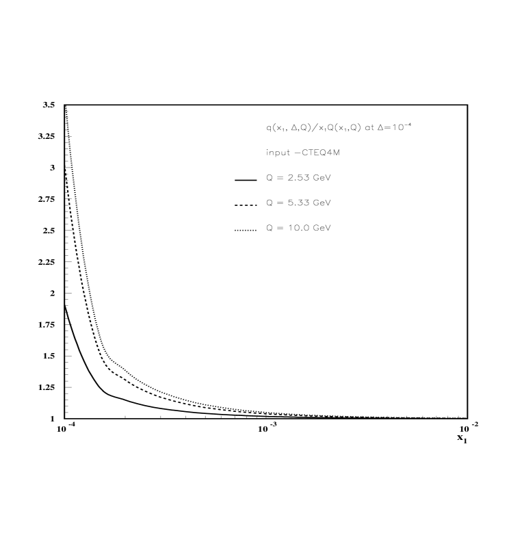
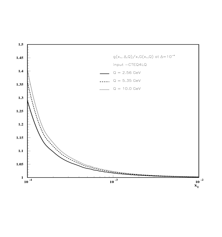
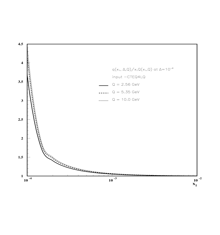
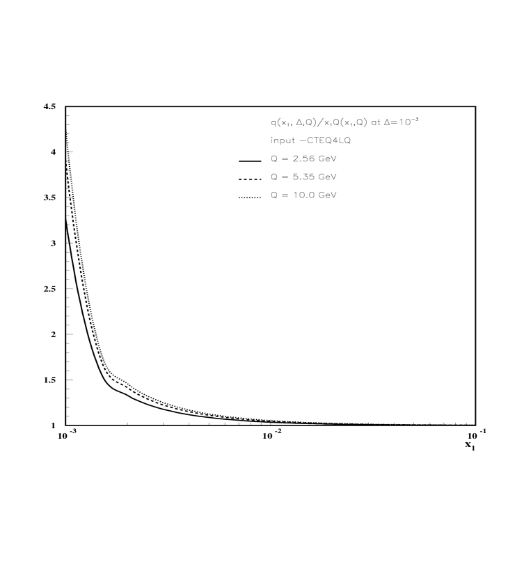
In the following figures (Fig. 2-7) we compare, for illustrative purposes, the diagonal and nondiagonal case by plotting the ratio
| (19) | |||
| (20) |
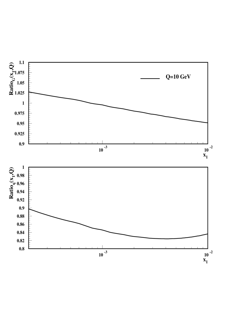
for various values of , and [27] , i.e. varying , using the CTEQ4M and CTEQ4LQ [28] parameterizations [30]. We assume the same initial conditions for the diagonal and nondiagonal case (see Ref. [5] for a detailed physical motivation of this ansatz).
The reader might wonder why only CTEQ4M and CTEQ4LQ and not GRV or MRS were used. The answer is not a prejudice of the authors against GRV or MRS but rather the fact that a comparison of CTEQ4M and CTEQ4LQ shows the same characteristic as comparing, for example, CTEQ4M and GRV at LO. The observation is the following: CTEQ4LQ is given at a different, rather low, , as compared to CTEQ4M and hence one has significant corrections from NLO terms in the evolution at these scales. This leads to a large difference between CTEQ4LQ and CTEQ4M (see Fig. 8), if one evolves the CTEQ4LQ set from its very low scale to the scale at which the CTEQ4M distribution is given, making a sensitivity study of nondiagonal parton distributions for different initial distributions impossible at LO. Of course, the inclusion of the NLO terms corrects this difference in the diagonal case but since there is no NLO calculation of the nondiagonal case available yet, a study of the sensitivity of nondiagonal evolution to different initial distributions has to wait.
The figures themselves suggest the following. The lower the starting scale, the stronger the effect of the difference of the nondiagonal evolution as compared to the diagonal one and also that most of the difference between nondiagonal and diagonal evolution stems from the first few steps in the evolution at lower scales. Secondly, under the assumption that the NLO evolution in the nondiagonal case will yield the same results for the parton distributions at some scale , irrespective of the starting scale , in analogy to the diagonal case. One can say that the NLO corrections to the nondiagonal evolution will be in the same direction and same order of magnitude as the diagonal NLO evolution. If, in the nondiagonal case, the NLO corrections were in the opposite direction, which would lead to a marked deviation from the LO results, compared to the diagonal case, the overall sign of the NLO nondiagonal kernels would have to change for some since in the limit we have to recover the diagonal case. This occurance is not likely for the following reason: First, the Feynaman diagrams involved in the calculation of the NLO nondiagonal kernels are the same as in the diagonal case, except for the different kinematics, therefore, we have a very good idea about the type of terms appearing in the kernels, namely polynomials, logs and terms in need of regularization such as . Moreover, the kernels, as stated before, have to reduce to the diagonal case in the limit of vanishing which fixes the sign of most terms in the kernel, thus the only type of terms which are allowed and could change the overall sign of the kernel are of the form
| (21) |
which will be numerically small unless in the convolution integral of the evolution equations. Moreover, we know that in this limit the contribution of the regularized terms in the kernel give the largest contributions in the convolution integral and therefore sign changing contributions in the nondiagonal case would have to originate from regularized terms. This in turn disallows a term like Eq. 21 due to the fact that regularized terms are not allowed to vanish in the diagonal limit, since the regularized terms arise from the same Feynman diagrams in the both diagonal and nondiagonal case. Therefore, the overall sign of the contribution of the NLO nondiagonal kernels will be the same as in the diagonal case.
A word should be said about how the results of Ref. [10] compare to ours. For the case of the same similar starting scales and almost identical values of we find good agreement with their numbers for at [29] and are slightly higher at larger . The observed differences are due to the fact that the quark distributions are included in our evolution as compared to [10] and their initial distributions is slightly different. We also find very similar ratios to [10] if one changes the starting scale to a lower one. The slight difference of a few percent in the ratios between us and [10] can again be attributed to the fact that they used the GRV distribution as compared to our use of the CTEQ4 distributions, hence a slight difference in the starting scales and their lack of incorporating quarks into the evolution.
V Conclusions
We modified the original CTEQ-code in such a way that we can now compute the evolution of nondiagonal parton distributions to LO. We gave a detailed account of the modifications and the methods employed in the new or modified subroutines. As the reader can see, the modifications and methods themselves are not something magical but rather a straightforward application of well known numerical methods. We further demonstrated the rapid convergence and stability of our code. In the limit of vanishing asymmetry we reproduce the diagonal case in LO as obtained from the original CTEQ-code within . We also have good agreement with the results in Ref. [10]. In the future, after the NLO kernels for the nondiagonal case have been calculated, we will extend the code to the NLO level to be on par with the diagonal case.
Acknowledgments
This work was supported in part by the U.S. Department of Energy under grant number DE-FG02-90ER-40577. We would like to thank John Collins and Mark Strikman for helpful conversations.
REFERENCES
- [1] S.J. Brodsky, L.L. Frankfurt, J.F. Gunion, A.H. Mueller, and M. Strikman, Phys. Rev. D50 (1994) 3134; see also [2]
- [2] L.L. Frankfurt, W. Koepf, and M. Strikman, Phys. Rev. D54 (1996) 3194.
- [3] A. Radyushkin Phys. Lett. B385 (1996) 333.
- [4] J.C. Collins, L. Frankfurt, and M. Strikman, Phys. Rev. D56 (1997) 2982.
- [5] L.L. Frankfurt, A. Freund, V. Guzey and M. Strikman, hep-ph/9703449 to appear in Phys. Lett. B.
- [6] X.-D. Ji, Phys. Rev. D55 (1997) 7114. .
- [7] A. Radyushkin Phys.Lett B380 (1996) 417, Phys. Rev. D56, 5524 (1997).
- [8] I.I Balitsky and V.M. Braun, Nucl. Phys. B311, 541 (1989).
- [9] J. Bluemlein, B. Geyer and D. Robaschik, hep-ph/9705264.
- [10] A.Martin and M.Ryskin, hep-ph/9711371.
- [11] L. Mankiewicz, G. Piller and T. Weigel, hep-ph/9711227.
- [12] D. Müller, hep-ph/9704406.
- [13] X. Ji and J. Osborne, hep-ph/9707254.
- [14] A.V. Belitsky and D. Müller, hep-ph/9709379.
- [15] M. Diehl, T. Gousset, B. Pire, and J.P. Ralston, Phys. Lett. B411, 193 (1997).
- [16] Z. Chen, hep-ph/9705279.
- [17] L. Frankfurt, A. Freund and M. Strikman, hep-ph/9710356.
- [18] L. Mankiewicz, G. Piller, E. Stein, M. Vättinen and T. Weigl, hep-ph/9712251.
- [19] J.C. Collins and A. Freund, hep-ph/9801262.
- [20] X.-D. Ji and J. Osborne, hep-ph/9801260.
- [21] For more details on the derivation of the kernels to leading order see for example [5, 6, 7].
- [22] The CTEQ-Meta page at http://www.phys.psu.edu/~cteq/ and the documentation in the different parts of the package.
- [23] The parton distributions functions are smooth and well behaved thus one just has to use enough points in .
- [24] The general analytic expressions for the convolution integrals in an arbitrary -bin were obtained with the help of MATHEMATICA.
- [25] The value of is specified in NINTEGR.
- [26] The value of the output at position is always since in this case the upper and the lower bound of the integral coincide.
- [27] We also plot the same ratio for to demonstrate the deviation from our code in the diagonal limit from the CTEQ-code.
- [28] CTEQ4LQ gives the best fit at low whereas CTEQ4M gives the best -fit for a large range of and .
- [29] This was also the case in Ref. [5] where the authors mistakenly put the energies as where in fact they should have been , which led to some confusion in the comparisons of this first study to Ref. [10].
- [30] H.L. Lai et al. Phys. Rev. D55 (1997) 1280.