Abstract

We study the spectrum of the reggeized gluon compound states in high-energy QCD. The energy of the states depends on the total set of quantum numbers whose values are constrained by the quantization conditions. To establish their explicit form we apply the methods of nonlinear WKB analysis to the Schrödinger equation for the $N$ reggeon state in the separated coordinates. We solve the quantization conditions for the $N=3$ reggeon states in the leading order of the WKB expansion and observe a good agreement of the obtained spectrum of quantum numbers with available exact solutions.

1. Introduction

In perturbative QCD analysis of the Regge asymptotics of hadronic scattering amplitudes, the power rise with energy of the physical cross-sections is attributed to the contribution of the color-singlet compound gluonic states. These states are built from an arbitrary conserved number, $N=2,3,...$, of reggeized gluons, or reggeons, and they can be defined as solutions of the effective $(2+1)-$dimensional Schrödinger equation [1]

$${\cal H}_{N}|{\chi_{N,\{q\}}}\rangle=E_{N,\{q\}}|{\chi_{N,\{q\}}}\rangle\,.$$ (1.1)

The effective QCD Hamiltonian ${\cal H}_{N}$ describes a pair-wise interaction between $N$ reggeons on the 2-dimensional plane of their transverse coordinates, $\vec{\rho}_{k}=(\rho_{x_{k}},\rho_{y_{k}})$ with $k=1$, $...$, $N$, and its explicit form can be found in [2]. The longitudinal gluonic degrees of freedom define the rapidity of reggeons that enter into (1.1) as a evolution time. The wave function $\chi_{N,\{q\}}(\vec{\rho}_{1}-\vec{\rho}_{0},...,\vec{\rho}_{N}-\vec{\rho}_{0})$ depends on some set of quantum numbers $\{q\}$ and the center-of-mass coordinate $\vec{\rho}_{0}$ of the reggeon compound state.

The contribution of the $N$ reggeon states to the physical cross section has a form

$$\sigma(s)\sim s^{\frac{\alpha_{\rm s}N_{c}}{2\pi}E_{N,\{q\}}}$$

and at large energies $s$ it is dominated by the state with the maximal energy, $E_{0}=\max_{\{q\}}E_{N,\{q\}}$. Therefore solving the Schrödinger equation (1.1) one is mostly interesting in finding the state with the energy $E_{0}$, or equivalently the ground state of the hamiltonian $-{\cal H}_{N}$.

The Schrödinger equation (1.1) has a number of remarkable properties. The effective QCD Hamiltonian ${\cal H}_{N}$ is invariant under projective $SL(2,\hbox{$\,\vrule height=6.45831pt,width=0.4pt,depth=0.0pt\kern-3.00003pt{\rm C}$})$ transformations of the 2-dimensional gluon coordinates $\rho_{j}$ [2]

$$z_{j}=\rho_{x_{j}}+i\rho_{y_{j}}\,,\qquad\bar{z}_{j}=z_{j}^{*}\,,\qquad z_{j}\to\frac{az_{j}+b}{cz_{j}+d}$$ (1.2)

with $ad-bc=1$ and $(z_{j},\bar{z}_{j})$ being (anti)holomorphic reggeon coordinates. Denoting the generators of these transformations as

$$L_{0}=\sum_{k=1}^{N}z_{k}\partial_{k}\,,\qquad L_{-}=\sum_{k=1}^{N}\partial_{k}\,,\qquad L_{+}=\sum_{k=1}^{N}z_{k}^{2}\partial_{k}\,,\qquad$$ (1.3)

and having similar expressions for the antiholomorphic generators, one may verify that $[{\cal H}_{N},L_{\alpha}]=[{\cal H}_{N},\bar{L}_{\alpha}]=0$. This symmetry allows to classify possible solutions to (1.1) according to the representations of the $SL(2,\hbox{$\,\vrule height=6.45831pt,width=0.4pt,depth=0.0pt\kern-3.00003pt{\rm C}$})$ group. In particular, the wave function is transformed under projective transformations as

$$\chi_{N,\{q\}}\to(cz_{0}+d)^{2h}(\bar{c}\bar{z}_{0}+\bar{d})^{2\bar{h}}\chi_{N,\{q\}}$$ (1.4)

with $(z_{0},\bar{z}_{0})$ being (anti)holomorphic coordinates of the center-of-mass. The conformal weights of the state, $h$ and $\bar{h}$, take the values corresponding to the unitary principal series representation of the $SL(2,\hbox{$\,\vrule height=6.45831pt,width=0.4pt,depth=0.0pt\kern-3.00003pt{\rm C}$})$ group [3]

$$h=\frac{1+n}{2}+i\nu\,,\qquad\bar{h}=\frac{1-n}{2}+i\nu\,,\qquad(n={\hbox{\cmss Z\kern-4.79993ptZ}}\,,\quad\nu={\hbox{{\rm I}\kern-1.99997pt\hbox{\rm R}}})$$ (1.5)

parameterized by the pair $(n,\nu)$ of integer $n$ and real $\nu$. These parameters determine the spin $s=n$ and the scaling dimension $d=1+2i\nu$ of the state and control the transformation properties of the state under rotations, $z_{k}\to\mathop{\rm e}\nolimits^{i\phi}z_{k}$, $\bar{z}_{k}\to\mathop{\rm e}\nolimits^{-i\phi}\bar{z}_{k}$, $\chi_{N}\to\mathop{\rm e}\nolimits^{in\phi}\chi_{N}$ and dilatations, $z_{k}\to\lambda z_{k}$, $\bar{z}_{k}\to\lambda\bar{z}_{k}$, $\chi_{N}\to\lambda^{-1-2i\nu}\chi_{N}$.

Being expressed in terms of holomorphic and antiholomorphic reggeon coordinates, the effective Hamiltonian splits into the sum of two mutually commuting $(1+1)-$dimensional Hamiltonians acting separately on (anti)holomorphic coordinates, ${\cal H}_{N}=H_{N}+\overline{H}_{N}$ and $[H_{N},\overline{H}_{N}]=0$ [4]. This property is exact for $N=2$ and $N=3$ reggeon states and for $N\geq 4$ it holds in the multi-color limit of QCD. It implies that the original equation (1.1) can be replaced by the system of two $(1+1)-$dimensional Schrödinger equations in holomorphic and antiholomorphic subspaces. As a result, the wave function of the state can be factorized as

$$\chi_{N}(z,\bar{z})=\sum_{\alpha}C_{\alpha}\,\varphi_{N,\alpha}(z)\bar{\varphi}_{N,\alpha}(\bar{z})\,,$$ (1.6)

where ${z}=(z_{1}-z_{0},...,z_{N}-z_{0})$ denotes the set of $N$ holomorphic coordinates and the coefficients $C_{\alpha}$ are fixed by the condition for $\chi_{N}(z,\bar{z})$ to be a well defined function of its arguments on the 2-dimensional plane of transverse coordinates. Additionally, the energy $E_{N}$ of the state can be evaluated as the sum of holomorphic and antiholomorphic energies that one finds solving two $(1+1)-$dimensional Schrödinger equations.

It turns out that the holomorphic Hamiltonian $H_{N}$ coincides with the Hamiltonian of 1-dimensional Heisenberg magnet of noncompact $SL(2,\hbox{$\,\vrule height=6.45831pt,width=0.4pt,depth=0.0pt\kern-3.00003pt{\rm C}$})$ spin zero [5, 6]. There is however an important difference between the holomorphic Hamiltonian $H_{N}$ and well-known integrable $(1+1)-$dimensional Hamiltonians [7, 8]. Examining the properties of $H_{N}$ one finds [9] that in contrast with the full $(2+1)-$dimensional effective Hamiltonian, the operator $H_{N}$ is unbounded on the space of the wave functions (1.4). The same property holds for the antiholomorphic hamiltonian $\overline{H}_{N}$. It is only the sum of holomorphic and antiholomorphic $(1+1)-$dimensional Hamiltonians that is bounded from above. This happens because the holomorphic and antiholomorphic energies depend on the common set of quantum numbers (1.5) and infinities cancel in their sum.

Analyzing the Schrödinger equation (1.1) one finds [5, 6] that it possesses the family of mutually commuting holomorphic and antiholomorphic integrals of motion, $\{q_{k},\bar{q}_{k}\}$, $k=2,...,N$ defined as

$$q_{k}=i^{k}\sum_{1\leq j_{1}<...<j_{k}\leq N}z_{j_{1}j_{2}}...z_{j_{k}j_{1}}\partial_{j_{1}}...\partial_{j_{k}}\,,\qquad\qquad[q_{k},{\cal H}_{N}]=0\,,$$ (1.7)

where $z_{jk}=z_{j}-z_{k}$ and the definition of the antiholomorphic charges $\bar{q}_{k}$ is similar with $z_{j}$ replaced by $\bar{z}_{j}$. The total number of the conserved charges, $2(N-1)$, is large enough for the $N-$gluon Schrödinger equation (1.1) to be completely integrable. The wave function of the $N-$reggeon state, $\chi_{N,\{q\}}$, diagonalizes these charges and one identifies the corresponding eigenvalues as a complete set of quantum numbers $\{q\}$ introduced before in (1.1). One also takes into account that on the space of the wave functions (1.4) the holomorphic and antiholomorphic charges are related as [9]

$$\bar{q}_{k}=q_{k}^{*}\,,\qquad k=2,...,N\,.$$

The integrability of the Schrödinger equation (1.1) ensures that the effective Hamiltonian ${\cal H}_{N}$ acting on the $2N$ coordinates of reggeons can be expressed as a complicated function of $2(N-1)$ integrals of motion $(q_{k},\bar{q}_{k})$ plus $2$ operators reserved for the components of the center-of-mass momentum of the state. We notice however that (anti)holomorphic components of the total momentum coincide with the generators, $L_{-}$ and $\bar{L}_{-}$, of the projective transformations (1.3) and the dependence of the Hamiltonian on them is protected by the $SL(2,\hbox{$\,\vrule height=6.45831pt,width=0.4pt,depth=0.0pt\kern-3.00003pt{\rm C}$})$ symmetry, $[{\cal H}_{N},L_{\alpha}]=0$. This leads to the following identity [9]

$$E_{N,\{q\}}=\varepsilon_{N}(q_{2},q_{3},...,q_{N})+\varepsilon_{N}(\bar{q}_{2},\bar{q}_{3},...,\bar{q}_{N})\,,$$

where $\varepsilon_{N}$ denotes the energy of the (anti)holomorphic Hamiltonian.

Thus, the problem of calculating the spectrum of the effective QCD Hamiltonian (1.1) is reduced, first, to finding the explicit form of $\varepsilon_{N}$ as a real function of the conserved charges $q_{2}$, $...$, $q_{N}$ and, second, to establishing the quantization conditions for their eigenvalues. The first part of the problem was studied using different approaches [10, 11] and similar results for $\varepsilon_{N}$ were obtained. In the present paper we address the problem of finding the spectrum of the conserved charges.

The paper is organized as follows. In the Sect. 2 we employ the WKB expansion to obtain the quantization conditions for the eigenvalues of conserved charges. We show in Sect. 3 that these conditions have the form of the Whitham equations. Solving the Whitham equations in the special case of $N=3$ reggeon states we obtain the quantized charges $q_{2}$ and $q_{3}$ and study their properties in Sect. 4. Concluding remarks can be found in Sect. 5. Appendix contains some properties of the elliptic integrals which are helpful in solving the Whitham equation.

2. Quantization conditions

The “lowest” integrals of motion, $q_{2}$ and $\bar{q}_{2}$, provide the simplest example of the quantization conditions. One verifies using (1.3) and (1.7) that $q_{2}$ and $\bar{q}_{2}$ coincide with the quadratic Casimir operators of the $SL(2,\hbox{$\,\vrule height=6.45831pt,width=0.4pt,depth=0.0pt\kern-3.00003pt{\rm C}$})$ group, $q_{2}=L_{0}(L_{0}+1)+L_{-}L_{+}$, and for the wave functions transforming as (1.4) their eigenvalues take the form

$$q_{2}=-h(h-1)=\frac{1}{4}-{\left({\frac{n}{2}+i\nu}\right)}^{2}\,,\qquad\bar{q}_{2}=-\bar{h}(\bar{h}-1)=q_{2}^{*}\,,$$ (2.1)

being discrete in $n$ and continuous in $\nu$. The quantization conditions for “higher” integrals of motion $q_{k}$ and $\bar{q}_{k}$ ($k\geq 3$) are more involved [9, 10]. One can get some insight into their properties by exploring the relation between the wave functions of reggeon compound states $\chi_{N}(z,\bar{z})$ and 2-dimensional conformal field theories. To this end, let us consider the following function [5, 10]

$$\widehat{\chi}_{N}(z,\bar{z})=(z_{12}z_{23}...z_{N1})^{-1}\chi_{N}(z,\bar{z})\,.$$

According to its properties under the projective transformations, (1.4), the function $\widehat{\chi}_{N}$ can be represented as $(N+1)-$point correlation function in 2-dimensional conformal field theory

$$\widehat{\chi}_{N}(z,\bar{z})=\left\langle{\phi(z_{1},\bar{z}_{1})...\phi(z_{N},\bar{z}_{N})O_{h,\bar{h}}(z_{0},\bar{z}_{0})}\right\rangle\,.$$ (2.2)

Here, $\phi(z,\bar{z})$ is a quasiprimary reggeon field with the conformal weights $(1,0)$ and $O_{h,\bar{h}}(z_{0},\bar{z}_{0})$ is a quasiprimary operator interpolating the $N$ reggeon compound state. The operator $O_{h,\bar{h}}$ has the conformal weights (1.5) and it is transformed under (1.2) according to the irreducible principal series representation (irreps) of the $SL(2,\hbox{$\,\vrule height=6.45831pt,width=0.4pt,depth=0.0pt\kern-3.00003pt{\rm C}$})$ group labeled as $t^{(\nu,2n)}$. For the reggeon operator $\phi(z,\bar{z})$ the corresponding irreps can be identified as $t^{(0,2)}$. The product of $N$ reggeon operators in (2.2) is reducible with respect to the action of the $SL(2,\hbox{$\,\vrule height=6.45831pt,width=0.4pt,depth=0.0pt\kern-3.00003pt{\rm C}$})$ transformations. It corresponds to the tensor product of $N$ copies of $t^{(0,2)}$ which in turn can be decomposed into irreducible components using the following fusion rules [3]

$$t^{(0,2)}\otimes t^{(0,2)}=\bigoplus_{n\in{\tiny\hbox{\rm Z}}\,,\nu\in{\tiny{\hbox{{\rm I}\kern-0.99998pt\hbox{\rm R}}}}}t^{(\nu,2n)}\,,\qquad t^{(\nu,2n)}\otimes t^{(0,2)}=\bigoplus_{m\in{\tiny\hbox{\rm Z}}\,,\rho\in{\tiny{\hbox{{\rm I}\kern-0.99998pt\hbox{\rm R}}}}}t^{(\rho,2m)}\,.$$

In conformal field theory these relations are implemented in the operator product expansion of the quasiprimary operators $\phi(z,\bar{z})$ and $O_{h,\bar{h}}(z,\bar{z})$ [12, 13]. Applying the fusion rules $N-1$ times one obtains an expansion of the product $\phi(z_{1},\bar{z}_{1})...\phi(z_{N},\bar{z}_{N})$ in (2.2) into an infinite sum of the irreducible components. Each component can be parameterized in two equivalent ways: either by the conformal weights $(h,\bar{h})$ plus the set of $2(N-2)$ quantum numbers $(q_{k},\bar{q}_{k})$, or by the set of $2(N-1)$ numbers $(n_{k},\nu_{k})$ corresponding to the $N-1$ intermediate states $t^{(\nu_{k},2n_{k})}$. This leads to the following dependence

$$q_{k}=q_{k}{\left({(n_{1},\nu_{1}),...,(n_{N-1},\nu_{N-1})}\right)}\,,\qquad(k=2,...,N)$$ (2.3)

together with $h=\frac{1+n_{N-1}}{2}+i\nu_{N-1}$ and $\bar{h}=1-h^{*}$. Thus, apart from the set $(n_{N-1},\nu_{N-1})$ defining the conformal weight of the $N$ reggeon state, one expects the appearance of $(N-2)$ additional sets $(n_{k},\nu_{k})$ parameterizing the eigenvalues of the operators $q_{k}$ and $\bar{q}_{k}$. In particular, for given conformal weights $(h,\bar{h})$ the possible values of the quantum numbers $q_{k}$ and $\bar{q}_{k}$ form the family of continuous functions of real $\nu_{1}$, $...$, $\nu_{N-2}$, different members of which are labeled by integers $n_{1}$, $...$, $n_{N-2}$.

Let us consider two special cases. In the first case, one takes all $\nu_{k}=0$ and $n_{k}={\rm odd}$. Using (1.5) one finds that it corresponds to restricting the conformal weights of the intermediate states $t^{(\nu_{k},2n_{k})}$ and the $N$ reggeon state, $t^{(\nu_{N-1},2n_{N-1})}$, to take only integer values. The spectrum of the operators $q_{k}$ and $\bar{q}_{k}$ is expected to be discrete. Indeed, this result was previously obtained within the algebraic Bethe Ansatz approach [5] by numerical solution of the Bethe equations [9] and later the analytical expressions for quantized $q_{k}$ and $\bar{q}_{k}$ were derived in the quasiclassical approximation [10]. In the second case, one chooses $n_{k}=0$ and $\nu_{k}$ are arbitrary. The conformal weights of the intermediate states have the form $h_{k}=\frac{1}{2}+i\nu_{k}$ and they run along imaginary axis. It has been argued [9] that it is for these values of the conformal weights that the energy of the $N$ reggeon states approaches its maximal value. The quantized $q_{k}$ and $\bar{q}_{k}$ become continuous functions of real $\nu_{1}$, $...$, $\nu_{N-1}$. As was shown in [14], these functions can be found within the WKB approach as solutions of the Whitham equations. In the next Section we derive these equations, solve them and study the properties of quantized $q_{k}$ and $\bar{q}_{k}$.

2.1. Separated variables

The eigenvalue problem for the operators $q_{k}$ and $\bar{q}_{k}$ defined in (1.7) leads to a complicated system of partial differential equations of the $N-$th order on the wave function $\chi_{N}$. One can significantly simplify the problem by using the fact that quantization of the charges $q_{k}$ and $\bar{q}_{k}$ does not depend on the particular representation in which the wave function $\chi_{N}$ is defined in order to go from $(z,\bar{z})-$coordinates to a new set of separated holomorphic reggeon coordinates [7, 8], $x_{1}$,…$x_{N}$, and their antiholomorphic counterparts $\bar{x}_{k}=x_{k}^{*}$.

In the separated coordinates the wave function of the $N$ reggeon state is factorized into the product of functions each depending on only one coordinate

$$\chi_{N}(x,\bar{x})=Q(x_{1})...Q(x_{N-1})\,x_{N}^{-h}\times\overline{Q}(\bar{x}_{1})...\overline{Q}(\bar{x}_{N-1})\,\bar{x}_{N}^{-\bar{h}}\,.$$ (2.4)

Here, the function $Q(x)$ is a solution of the second order finite-difference equation [5]

$$Q(x+i)+Q(x-i)=x^{-N}\Lambda(x)Q(x)\,,\qquad\Lambda(x)=2x^{N}+q_{2}x^{N-2}+...+q_{N}$$ (2.5)

known as the Baxter equation and $\overline{Q}(x)$ satisfies similar relation with all $q_{k}$ replaced by $\bar{q}_{k}=q_{k}^{*}$.

The separated gluon coordinates have the following properties. The coordinates $x_{N}$ and $\bar{x}_{N}$ correspond to the center-of-mass motion and they are defined as eigenvalues of the operators

$$x_{N}=L_{0}L_{-}^{-1}\,,\qquad\bar{x}_{N}=\bar{L}_{0}\bar{L}_{-}^{-1}$$ (2.6)

with $L_{-}$ and $L_{0}$ being the $SL(2,\hbox{$\,\vrule height=6.45831pt,width=0.4pt,depth=0.0pt\kern-3.00003pt{\rm C}$})$ generators (1.3). The definition of the remaining coordinates $x_{k}$ and $\bar{x}_{k}$ for $k=1,..,N-1$ is more involved and it can be found in [9, 7]. It will be important for us that they satisfy the relations [7]

$$[L_{0},x_{k}]=[L_{-},x_{k}]=0\,,\qquad[L_{0},x_{N}]=ix_{N}\,,\qquad[L_{-},x_{N}]=-i$$

with $k=1$, $...$, $N-1$ and similar relations hold for $\bar{x}_{k}$ and $\bar{x}_{N}$. From these relations one finds that the separated coordinates $x_{k}$ and $\bar{x}_{k}$, being functions of the gluon $(z_{j},\bar{z}_{j})-$coordinates, are invariant under translations, $z_{k}\to z_{k}+\epsilon$, and dilatations, $z_{k}\to\lambda z_{k}$, while the coordinates $x_{N}$ and $\bar{x}_{N}$ are transformed in the same way as $z_{k}$ and $\bar{z}_{k}$. Therefore, in the expression (2.4) for the wave function in separated coordinates, it is the factor $x_{N}^{-h}\bar{x}_{N}^{-\bar{h}}$ that carries the spin $n=h-\bar{h}$ and the scaling dimension $d=1+2i\nu=h+\bar{h}$ of the $N$ reggeon state. Moreover, making the shift, $z_{k}\to z_{k}-z_{0}$, one can restore the dependence of the wave function (2.4) on the center-of-mass coordinate of the state, $(z_{0},\bar{z}_{0})$, as $x_{N}\to x_{N}-z_{0}$ and $x_{k}\to x_{k}$ $(k=1,...,N-1)$.

The wave function (1.6) has to be a well defined function of the reggeon coordinates $z_{k}$ and $\bar{z}_{k}$. Performing transition to the separated coordinates one imposes the same condition on (2.4) as a function of the complex $x_{k}$ and $\bar{x}_{k}=x_{k}^{*}$. Let us first examine the dependence of $\chi_{N}$ on the coordinate $x_{N}$. If $\chi_{N}$ is a single valued function of complex $x_{N}$ it should not be changed as $x_{N}\to\mathop{\rm e}\nolimits^{2\pi i}x_{N}$ in (2.4). One checks that this is true provided that the spin $h-\bar{h}=n$ of the state is integer. Requiring additionally that the scaling dimension of the state has to be $d=h+\bar{h}=1+2i\nu$ one reproduces the quantization conditions (1.5) for the conformal weights. We notice that although the wave function (2.4) stays invariant under $2\pi$ rotations on the $x_{N}-$plane, its holomorphic and antiholomorphic components get nontrivial monodromies for all values of the conformal weights $h$ and $\bar{h}$ except for integer ones. The latter case corresponds to the polynomial solutions studied in [9, 10].

To satisfy the condition of singlevaluedness for the dependence of (2.4) on the remaining coordinates $x_{k}$ one has to examine the properties of the product $Q(x)\overline{Q}(x^{*})$ on the complex $x-$plane. As we will show below, this consideration leads to the selection rules for the quantum numbers $q_{3}$, $...$, $q_{N}$

2.2. Properties of the Baxter equation

The function $Q(x)$ entering (2.4) obeys the Baxter equation (2.5). This equation has two linear independent solutions, $Q_{+}(x)$ and $Q_{-}(x)$, satisfying the normalization condition

$$W(x)=Q_{+}(x+i)Q_{-}(x)-Q_{-}(x+i)Q_{+}(x)=1$$

and having the following asymptotics at infinity

$$Q_{+}(x)\sim x^{h}\,,\qquad Q_{-}(x)\sim x^{1-h}\qquad\mbox{as $x\to\infty$}\,.$$ (2.7)

The analysis of the Baxter equation for the function $\overline{Q}(\bar{x})$ is similar since the functions $(Q(x))^{*}$ and $\overline{Q}(x^{*})$ satisfy the same equation. As a result, one gets the following general expression

$$Q(x)\overline{Q}(x^{*})=\sum_{\alpha,\beta=\pm}C_{\alpha\beta}\,Q_{\alpha}(x)(Q_{\beta}(x))^{*}$$

with $C_{\alpha\beta}$ being arbitrary coefficients. However, it follows from (2.7) that for the conformal weights $h$ and $\bar{h}$ of the form (1.5) the functions $Q_{+}(x)$ and $Q_{-}(x)$ acquire nontrivial monodromies at infinity as $x\to\mathop{\rm e}\nolimits^{2\pi i}x$, which should cancel in the product $Q(x)\overline{Q}(x^{*})$. This requirement leads to $C_{--}=C_{++}=0$ and

$$Q(x)\overline{Q}(x^{*})=C_{+-}Q_{+}(x)(Q_{-}(x))^{*}+C_{-+}Q_{-}(x)(Q_{+}(x))^{*}\,.$$ (2.8)

with $C_{+-}$ and $C_{-+}$ being some constants.

The asymptotic behaviour (2.7) of the functions $Q_{\pm}(x)$ is fixed by the conformal weight of the state and it is not sensitive to the value of “higher” quantum numbers $q_{3}$, $...$, $q_{N}$. To obtain the quantization conditions for $q_{3}$, $...$, $q_{N}$ one has to identify the remaining singularities of the solutions of the Baxter equation, $Q_{+}(x)$ and $Q_{-}(x)$, on the complex $x-$plane and examine the monodromy of $Q_{+}(x)(Q_{-}(x))^{*}$ around them.

As an example, let us seek for solutions $Q(x)$ to the Baxter equation within the class of rational functions. The distinguished property of such solutions is that they have a finite number of poles on the $x-$plane and scale at infinity as an integer power of $x$. According to (2.7) the latter property implies integer values of the conformal weight $h$. Then, straightforward analysis shows that $Q(x)$ can not have poles on the $x-$plane, since otherwise in order to balance the both sides of the Baxter equation (2.5) the functions $Q(x)$ should have an infinite sequence of poles shifted by $\pm i$ along imaginary axis. In similar manner, taking the limit $x\to 0$ in (2.5) one can argue that $Q(x)$ should vanish at the origin faster then $x^{N}$. These two conditions fix $Q(x)$ to be a polynomial of degree $h\geq N$ with $N-$times degenerate root $x=0$

$$Q_{+}(x)=x^{N}\prod_{k=1}^{h-N}(x-\lambda_{k})\,.$$ (2.9)

The remaining $h-N$ roots of the polynomial, $\lambda_{k}$, satisfy the Bethe equations and for given $h$ they take a discrete set of real values [5, 9]. Substituting this solution back into the Baxter equation (2.5) and comparing its both sides one can express quantized $q_{k}$ in terms of the roots. The spectrum of $q_{k}$ takes the form (2.3) with $\nu_{k}=0$ and $n_{k}=\rm odd$ and it can be calculated explicitly [9]. Thus defined polynomial solutions of the Baxter equation were first obtained within the algebraic Bethe Ansatz approach and their properties were studied in detail [9, 10].

To find the most general form of the quantization conditions (2.3) one has to solve the Baxter equation (2.5) for arbitrary complex conformal weights of the form (1.5). Different attempts have been undertaken [15, 10, 16], but the analytical solution similar to (2.9) is not available at present. As the first approximation to the exact solution, it has been proposed [14] to look for the asymptotic solution to the Baxter equation by applying the methods of nonlinear WKB analysis well-known from the studies of the Painlevé type-I equation [17].

2.3. WKB expansion

Let us interpret the Baxter equation (2.5) as a 1-dimensional discretized Schrödinger equation on the complex $x-$line and let us look for its solutions in the form of the WKB expansion. One observes that the Planck constant is formally unity $\hbar=1$ in the Baxter equation and the quasiclassical limit corresponds to large values of the “energies” $q_{k}$ entering into the definition (2.5) of $\Lambda(x)$. This limit can be effectively performed by introducing an arbitrary small parameter $\eta$ and rescaling the coordinate, $x\to x/\eta$, and the quantum numbers, $q_{k}\to q_{k}\eta^{k}$, in (2.5). Then, the asymptotic solution to the Baxter equation has the form [18, 10, 14]

$$Q(x/\eta)=\exp{\left({\frac{i}{\eta}\int^{x}dS(x)}\right)}\,,\qquad S(x)=S_{0}(x)+\eta S_{1}(x)+{\cal O}(\eta^{2})\,,$$ (2.10)

where $S_{0}(x)$ and $S_{1}(x)$ satisfy the relations

$$2\cosh S_{0}^{\prime}(x)=\frac{\widehat{\Lambda}(x)}{x^{N}}\,,\qquad S_{1}^{\prime}(x)=\frac{i}{2}\frac{d}{dx}\ln\sinh S_{0}^{\prime}(x)$$ (2.11)

with $S^{\prime}(x)=\partial_{x}S(x)$ and

$$\widehat{\Lambda}(x)=2x^{N}+\widehat{q}_{2}x^{N-2}+...+\widehat{q}_{N}\,,\qquad\widehat{q}_{k}\equiv q_{k}\eta^{k}={\rm fixed}\quad\mbox{as $\eta\to 0$}\,.$$ (2.12)

Similar expressions can be obtained for the antiholomorphic solution $\overline{Q}(x)$.

The limit $\eta\to 0$, or equivalently $q_{k}={\rm large}$, is an analog of the classical limit in quantum mechanics. As $\eta\to 0$ the quantum fluctuations become frozen and the motion of particles is restricted to their classical trajectories defined by the leading term in (2.10), the eikonal phase $S_{0}(x)$. Having identified $\sum_{k}S_{0}(x_{k})$ as the “action” function for the system of $N$ reggeons in the separated coordinates one may find the classical trajectories of gluons generated by the “classical” Hamiltonians $q_{k}$ by solving the system of the corresponding Hamilton-Jacobi equations. This system of equations is exactly integrable and its solutions can be described as cycles on the Riemann surface $\Gamma_{N}$ in the following way [19, 14].

Let us introduce the algebraic curve $\Gamma_{N}$

$$\Gamma_{N}:\qquad y^{2}=\widehat{\Lambda}^{2}(x)-4x^{2N}\,,$$ (2.13)

with $\widehat{\Lambda}(x)$ given by (2.12). This relation defines $y=y(x)$ as a double-valued function on the complex $x-$plane having $2N-2$ branching points at $x=\sigma_{j}$ such that $y(\sigma_{j})=0$ or

$$\widehat{\Lambda}^{2}(\sigma_{j})=4\sigma_{j}^{2N}\,.$$ (2.14)

The same function becomes a single-valued on the Riemann surface $\Gamma_{N}$ obtained by gluing together two sheets of the $x-$plane along the cuts $[\sigma_{2j},\sigma_{2j+1}]$, $j=1,...,N-1$ running between the branching points. Encircling the cuts by oriented closed contours one constructs the set of $N-1$ cycles $\alpha_{1}$, $...$, $\alpha_{N-1}$. The genus of $\Gamma_{N}$ equals $N-2$ and it depends on the number of reggeons “inside” the compound state.

The classical trajectories of reggeons in the separated coordinates $x_{1}$, $...$, $x_{N-1}$ correspond to the independent motion along $N-1$ different $\alpha-$cycles on the Riemann surface $\Gamma_{N}$. The branching points of $\Gamma_{N}$ become the turning points of the reggeon trajectories. Coming back from the separated coordinates to the original reggeon coordinates, $z_{k}$ and $\bar{z}_{k}$, one can show that the same motion looks on the 2-dimensional plane of transverse gluon coordinates as a soliton wave propagating in the system of $N$ interacting gluons [14]. Its explicit expression was constructed in [20] using the methods of the finite-gap theory out of the curve $\Gamma_{N}$. The quantum numbers of the $N$ reggeon state, $q_{k}$, become parameters of the soliton solutions. The quantization of $q_{k}$ appears as a result of imposing the Bohr-Sommerfeld quantization conditions on the periodic reggeon trajectories in the action-angle variables $(a_{k},\varphi_{k})$ defined as [19]

$$a_{k}=\frac{1}{2\pi}\oint_{\alpha_{k}}dS_{0}(x)\,,\qquad\varphi_{k}=\frac{\partial S_{0}(x)}{\partial a_{k}}\,,$$ (2.15)

where $0\leq\varphi_{k}\leq 2\pi$ and $\alpha_{k}$ are cycles on the Riemann surface (2.13).

To establish the explicit form of the WKB quantization conditions let us consider the properties of the differential $dS=dS_{0}(x)+\eta dS_{1}(x)+{\cal O}(\eta^{2})$ defined by the WKB ansatz (2.10). One finds from (2.11) that $dS_{0}$ is the following meromorphic differential on $\Gamma_{N}$

$$dS_{0}(x)=dx\ln\omega(x)\simeq\frac{dx}{y}\left[N\widehat{\Lambda}(x)-x\widehat{\Lambda}^{\prime}(x)\right].$$ (2.16)

Here the notation was introduced for the curve $\omega=\omega(x)$

$$\omega+1/{\omega}=\widehat{\Lambda}(x)/x^{N}\,,\qquad y=x^{N}{\left({\omega-1/{\omega}}\right)}$$ (2.17)

and the sign $\simeq$ means equivalence up to the exact differential, $d(x\ln\omega)$, having vanishing $\alpha-$periods.

Solving (2.11) we obtain two different solutions, $dS_{0,+}(x)$ and $dS_{0,-}(x)$, which are continuous functions of complex $x$ except across the cuts $[\sigma_{2j},\sigma_{2j+1}]$, satisfying the relation $dS_{0,+}(x)=-dS_{0,-}(x)$. Being combined together they define the differential $dS_{0}(x)$ as a double-valued function on the complex $x-$plane. Nevertheless, $dS_{0}$ is a single-valued function on the Riemann surface $\Gamma_{N}$ built from two copies of the $x-$plane to which we will refer as upper and lower sheets. Examining (2.11) as $x\to\infty$ we obtain the behaviour of $dS_{0}(x)$ on the upper, $dS_{0,+}$, and lower, $dS_{0,-}$, sheets of $\Gamma_{N}$ as

$$dS_{0,\pm}(x)\sim\pm i\eta\sqrt{-q_{2}}\frac{dx}{x}\,,\qquad\mbox{as $x\to\infty$}\,,$$ (2.18)

where $q_{2}$ is given by (2.1).

The first nonleading correction to the WKB phase $S(x)$ is defined by the differential $dS_{1}$ which one calculates using (2.16) and (2.17) as

$$dS_{1}(x)=\frac{i}{4}d\ln\frac{\widehat{\Lambda}^{2}(x)-4x^{2n}}{4x^{2N}}=\frac{i}{4}dx{\left({\sum_{k=1}^{2N-2}\frac{1}{x-\sigma_{k}}-\frac{2N}{x}}\right)}$$ (2.19)

with $\sigma_{k}$ being the branching points (2.14). In contrast with $dS_{0}$, this differential is well defined on the complex $x-$plane. It has poles located at the branching points (2.14), at the origin and at the infinity where its asymptotics is given by

$$dS_{1}(x)\sim-\frac{i}{2}\frac{dx}{x}\,,\qquad\mbox{as $x\to\infty$}\,.$$ (2.20)

Combining together (2.16) and (2.19) we find that two different branches of the differential $dS_{0}$ give rise to two linear independent WKB solutions to the Baxter equation

$$Q_{\pm}(x/\eta)\equiv\exp{\left({\frac{i}{\eta}\int^{x}dS_{\pm}(x)}\right)}\,,$$

where

$$dS_{+}(x) = dS_{0,+}(x)+\eta dS_{1}(x)+{\cal O}(\eta^{2})\,,$$

$$dS_{-}(x) = dS_{0,-}(x)+\eta dS_{1}(x)+{\cal O}(\eta^{2})=-dS_{0,+}(x)+\eta dS_{1}+{\cal O}(\eta^{2})\,.$$

Their asymptotics at infinity can be obtained from (2.18) and (2.20) as

$$dS_{\pm}(x)=-i\eta\frac{dx}{x}{\left({\pm\sqrt{-q_{2}}+\frac{1}{2}+{\cal O}(\eta)}\right)}\,.$$

We recall that at small $\eta$ the quantum numbers $q_{k}$ scale as $q_{k}\sim 1/\eta^{k}$. Therefore, replacing $\sqrt{-q_{2}}=h-\frac{1}{2}+{\cal O}(h^{-2})$ and taking the limit $\eta\to 0$ one checks that the functions $Q_{\pm}(x/\eta)$ behave at infinity in accordance with (2.7).

Substituting the obtained WKB expressions for $Q_{\pm}(x/\eta)$ into (2.8) and keeping only the first term in the r.h.s. of (2.8) one finds the holomorphic and antiholomorphic WKB solutions to the Baxter equation as

$$Q(x/\eta) = \exp\left\{\frac{i}{\eta}\int^{x}dS_{0,+}+i\int^{x}dS_{1}+{\cal O}(\eta)\right\}$$ (2.21)

$$\overline{Q}(x^{*}/\eta) = \exp\left\{\frac{i}{\eta}{\left({\int^{x}dS_{0,+}}\right)}^{*}-i{\left({\int^{x}dS_{1}}\right)}^{*}+{\cal O}(\eta)\right\}\,.$$

Let us examine the analytical properties of these functions on the complex $x-$plane. Relations (2.16) and (2.19) imply that the singularities of both functions are located on the cuts $[\sigma_{2k},\sigma_{2k+1}]$. For the product $Q(x/\eta)\overline{Q}(x^{*}/\eta)$ to be a uniform function of $x$ one has to require that for $x$ encircling the cuts $[\sigma_{2k},\sigma_{2k+1}]$ on the complex plane along the cycles $\alpha_{k}$ it should come to the starting point with the same value. This gives the following set of $N-1$ quantization conditions

$$\mathop{\rm Re}\nolimits{\left({\oint_{\alpha_{k}}dS_{0,+}}\right)}-\eta\mathop{\rm Im}\nolimits{\left({\oint_{\alpha_{k}}dS_{1}}\right)}+{\cal O}(\eta^{2})=\eta\pi n_{k}$$ (2.22)

where $n_{k}$ $(k=1,...,N-1)$ are integers and ${\cal O}(\eta^{2})$ stands for nonleading terms in the WKB expansion. According to (2.19), the differential $dS_{1}$ has poles on the $x-$plane and the calculation of its $\alpha-$periods is reduced to taking the residues at the poles located inside $\alpha_{k}$. Since by definition each $\alpha-$cycle encircles two branching points, $\sigma_{2k}$ and $\sigma_{2k+1}$, and, additionally, one of the cycles, say $\alpha_{k_{0}}$, encircles the pole at $x=0$, one gets

$$\frac{1}{2\pi}\oint_{\alpha_{k}}dS_{1}=-\frac{1}{2}+\delta_{k,k_{0}}\frac{N}{2}\,.$$ (2.23)

Substituting this expression into (2.22) we write the quantization condition in the following form

$$\frac{1}{2\pi}\oint_{\alpha_{k}}dS_{0,+}(x)=\eta\,{\left({\frac{n_{k}}{2}+i\nu_{k}}\right)}+{\cal O}(\eta^{2})\,,$$ (2.24)

with $\nu_{k}$ $(k=1,...,N-1)$ being arbitrary real numbers. This relation has a simple interpretation in terms of the action variables (2.15). Namely, it states that the possible values of the action variables $a_{k}$ match into the spectrum of the conformal weights (1.5) of the principal series representation of the $SL(2,\hbox{$\,\vrule height=6.45831pt,width=0.4pt,depth=0.0pt\kern-3.00003pt{\rm C}$})$ group.

The periods of the differential $dS_{0,+}$ entering the l.h.s. of the quantization conditions (2.24) are uniquely defined by the values of the quantum numbers $q_{2}$, $...$, $q_{N}$. Therefore, solving the system of $N-1$ equations (2.24), one will get $q_{2}$, $...$, $q_{N}$ as functions of $N-1$ complex numbers $\ell_{k}=\frac{n_{k}}{2}+i\nu_{k}$, each corresponding to $N-1$ cycles on the Riemann surface $\Gamma_{N}$. This result is in agreement with our expectations (2.3) and, additionally, it implies that the WKB quantized $q_{k}$ are holomorphic functions of $\ell_{k}$

$$q_{k}=q_{k}(\ell_{1},...,\ell_{N-1})\,,\qquad\ell_{k}=\frac{n_{k}}{2}+i\nu_{k}\,.$$ (2.25)

The same parameters determine the value of the conformal weight $h$ as follows. One takes into account that the sum of the $\alpha-$periods of the differential $dS_{0,+}$ is equal to its period around the infinity where the differential has a simple pole (2.18) with the residue $\eta\sqrt{-q_{2}}$. In this way one gets using (2.24)

$$\sqrt{-q_{2}}=\sum_{k=1}^{N-1}{\left({\frac{n_{k}}{2}+i\nu_{k}}\right)}+{\cal O}(\eta)$$ (2.26)

with $\eta\sim 1/\sqrt{-q_{2}}$. For large $-q_{2}$, or equivalently large conformal weights $h$, one replaces $\sqrt{-q_{2}}=h-\frac{1}{2}+{\cal O}(1/h)$ to obtain the expression for $h$ which reproduces possible quantized values of the conformal weight (1.5) with $n=\sum_{k}n_{k}$ and $\nu=\sum_{k}\nu_{k}$.

Having defined in (2.23) and (2.24) the periods of the differentials, one calculates the monodromy of the WKB solutions to the Baxter equation, (2.21), along the $\alpha_{k}-$cycles as

$$Q(x)\stackrel{{\scriptstyle x\circlearrowleft\alpha_{k}}}{{\longrightarrow}}Q(x)\mathop{\rm e}\nolimits^{2\pi i{\left({\frac{n_{k}-1}{2}+i\nu_{k}+\frac{N}{2}\delta_{k,k_{0}}}\right)}}\,,\qquad\overline{Q}(x^{*})\stackrel{{\scriptstyle x\circlearrowleft\alpha_{k}}}{{\longrightarrow}}\overline{Q}(x^{*})\mathop{\rm e}\nolimits^{2\pi i{\left({\frac{n_{k}+1}{2}-i\nu_{k}-\frac{N}{2}\delta_{k,k_{0}}}\right)}}\,,$$ (2.27)

where higher order WKB corrections were neglected. One verifies that the monodromies cancel against each other in the product $Q(x)\overline{Q}(x^{*})$. Moreover, moving $x$ around all $\alpha-$cycles on the complex $x-$plane and subsequently applying (2.27) one reproduces the monodromy at infinity

$$Q(x)\to Q(x)\mathop{\rm e}\nolimits^{2\pi ih}\,,\qquad\overline{Q}(x^{*})\to\overline{Q}(x^{*})\mathop{\rm e}\nolimits^{2\pi i(1-h^{*})}\,.$$

Relations (2.27) allow us to establish the correspondence between WKB quantization conditions (2.24) and the special class of exact polynomial solutions to the Baxter equation (2.9). Namely, comparing (2.27) with (2.9) one has to require that $\exp({2\pi i{\left({\frac{n_{k}-1}{2}+i\nu_{k}+\frac{N}{2}\delta_{k,k_{0}}}\right)}})=1$. This leads to the additional constraints on the parameters of the WKB quantization conditions (2.24):

$$\nu_{k}=0\,,\qquad n_{k}+\delta_{k,k_{0}}N=2{\hbox{\cmss Z\kern-4.79993ptZ}}_{+}+1$$

and, as a consequence, the conformal weight $h=\frac{1}{2}+\sum_{j}\frac{n_{j}}{2}+i\nu_{j}$ takes only positive integer values. The resulting quantization conditions were studied in [10, 14] and their solutions, $q_{k}$, were found to be in a good agreement with numerical calculations within the algebraic Bethe Ansatz approach [9].

3. Whitham flow

Let us apply the quantization conditions (2.24) to obtain the expressions for the charges $q_{3}$, $...$, $q_{N}$ in the leading order of the WKB expansion. In the leading order one neglects ${\cal O}(\eta^{2})-$corrections to (2.24) and uses invariance of the differential (2.16) and the curve (2.13) under transformations

$$x\to\lambda x\,,\qquad\widehat{q}_{k}\to\lambda^{k}\widehat{q}_{k}\,,\qquad dS_{0}\to\lambda dS_{0}$$

induced by reparameterization of the WKB expansion parameter, $\eta\to\lambda\eta$, to put $\eta=1/\sqrt{-q_{2}}$, or equivalently $\widehat{q}_{2}=-1$, in (2.24). This amounts to replacing $\widehat{q}_{k}$ in the definition, (2.12) and (2.16), of the differential $dS_{0}$ by invariant parameters

$$u_{k}=q_{k}/(-q_{2})^{k/2}\,,\qquad k=3,...,N\,,$$ (3.1)

called the moduli of the curve $\Gamma_{N}$. One also introduces notation for the r.h.s. of (2.24) as

$$\delta_{k}=\frac{\frac{n_{k}}{2}+i\nu_{k}}{\sqrt{-q_{2}}}\,,\qquad\quad\sum_{k=1}^{N-1}\delta_{k}=1\,,$$ (3.2)

where the last relation follows from (2.26).

In terms of new variables the quantization conditions (2.24) become the relations between the moduli $u_{k}$ and the parameters $\delta_{j}$. In particular, in the case of $N=3$ states the quantization conditions for the moduli $u_{3}\equiv u$ look like

$$\oint_{\alpha_{k}}\frac{(3u-2x)dx}{\sqrt{(u-x)(4x^{3}-x+u)}}=2\pi\delta_{k}\,,\qquad k=1\,,2\,.$$ (3.3)

Solving (3.3) and (2.24) one finds the moduli, $u_{k}=u_{k}(\delta_{1},...,\delta_{N-1})$, as smooth functions of the complex parameters $\delta_{k}$ and then calculates the corresponding values of the quantum numbers $q_{3}$, $...$, $q_{N}$ using (3.1) and (3.2).

Let us consider the relations (3.1) and (3.2) in two special cases discussed before Sect.2.1: $n_{k}=0$, $\nu_{k}\neq 0$ and $n_{k}\neq 0$, $\nu_{k}=0$ for all $k$, to which we will refer below as I and II, respectively. We find that in both cases the parameters (3.2) take real values

$$\delta^{\rm(I)}_{k}=\frac{\nu_{k}}{\nu_{1}+...+\nu_{N-1}}\,,\qquad\quad\delta^{\rm(II)}_{k}=\frac{n_{k}}{n_{1}+...+n_{N-1}}\,.$$

They are discrete for $\delta^{\rm(II)}_{k}$ and continuous for $\delta^{\rm(I)}_{k}$ with the former being the subset of the latter. Calculating the moduli as $u^{\rm(I)}_{k}=u_{k}(\delta^{\rm(I)})$ and $u^{\rm(II)}_{k}=u_{k}(\delta^{\rm(II)})$ one realizes that they enjoy the same properties. Among other things this means that in both cases the moduli are universal, that is they are given by the values of same function $u=u(\delta)$ on the real $\delta-$axis. In particular, this function can be calculated for real $\delta$ in the case II using available exact polynomial solutions of the Baxter equation and then applied to evaluate the quantized $q_{k}$ in the case I.

Universality of moduli leads to the following expressions for the quantum numbers (3.1) and (3.2)

$$q_{2}^{\rm(I)}=-(i\nu)^{2}\,,\qquad\quad q_{k}^{\rm(I)}=(i\nu)^{k}u_{k}{\left({\frac{\nu_{1}}{\nu},...,\frac{\nu_{N-1}}{\nu}}\right)}$$ (3.4)

and

$$q_{2}^{\rm(II)}=-{\left({\frac{n}{2}}\right)}^{2}\,,\qquad\quad q_{k}^{\rm(II)}={\left({\frac{n}{2}}\right)}^{k}u_{k}{\left({\frac{n_{1}}{n},...,\frac{n_{N-1}}{n}}\right)}$$ (3.5)

with $\nu=\sum_{k=1}^{N-1}\nu_{k}$ and $n=\sum_{k=1}^{N-1}n_{k}$. One notices that the substitution

$$\frac{n_{k}}{2}\rightleftharpoons i\nu_{k}$$

maps one of the relations into another one and the same transformation leaves invariant the expression (2.25) and the quantization conditions (2.24).

We would like to stress that the relations (3.4) and (3.5) were obtained in the leading order of the WKB expansion and they are valid for large $n$ and $\nu$. In this limit, one finds using (2.1) that the conformal weight has the form

$$h^{\rm(I)}=\frac{1}{2}+i\nu\,,\qquad\quad h^{\rm(II)}=\frac{1}{2}+\frac{n}{2}\,,$$ (3.6)

which is in agreement with the general expression (1.5). In the case II for $n={\rm odd}$ one compares (3.5) with the results of the polynomial solutions of the Baxter equation [10] to deduce that the quantized $q_{k}^{\rm(II)}$ take real values. As a consequence, $u_{k}$ is a real function of its arguments. Applying this property to (3.4) one finds that the quantum numbers $q_{k}^{\rm(I)}$ are real for even $k$ and pure imaginary for odd $k$. It is for these values of the quantun numbers that one expects to find the state in the spectrum of the effective QCD Hamiltonian (1.1) with the maximal energy [11].

3.1. Whitham equations

Let us solve the quantization conditions (2.24) and (3.3) and determine the functions $u_{k}$. The remarkable property of the moduli $u_{k}$ is that their dependence on $\delta_{j}$ is governed by the Whitham equations [21]. To derive these equations one varies the both sides of the quantization conditions (2.24) with respect to $\delta_{k}$ and observes the following property of the differential (2.16)

$$\frac{\partial dS_{0}}{\partial\delta_{k}}=\frac{dx}{\omega}\frac{\partial\omega}{\partial\delta_{k}}=\frac{dx}{y}\frac{\partial\widehat{\Lambda}(x)}{\partial\delta_{k}}=\frac{dx}{y}\sum_{j=3}^{N}x^{N-j}\frac{\partial u_{j}}{\partial\delta_{k}}\,,$$

where $\widehat{\Lambda}(x)=2x^{N}-x^{N-2}+u_{3}x^{N-3}+...+u_{N}$ and the relation (2.17) was used. This leads the following system of Whitham equations [14]

$$\frac{\partial u_{j}}{\partial\delta_{k}}=U_{kj}(u_{3},...,u_{N})\,,$$ (3.7)

with $j=3,...,N$, $k=1,...,N-1$ and $U_{kj}$ being the matrix inverse to

$${\left({U^{-1}}\right)}_{jk}=\frac{1}{2\pi}\oint_{\alpha_{k}}\frac{dx\,x^{N-j}}{\sqrt{\widehat{\Lambda}^{2}(x)-4x^{2N}}}\,.$$

The Whitham equations have the following interpretation [21] in terms of “classical” reggeon trajectories defined by the action function $S_{0}(x)$. The moduli $u_{k}$ enter as parameters into the classical soliton wave solutions of the Hamilton-Jacobi equations. Equations (3.7) describe the flow of the moduli $u_{k}$ in the slow “times” $\delta_{1}$, $...$, $\delta_{N-1}$, corresponding to adiabatic deformations of the soliton waves propagating in the system of $N$ reggeons.

Analysis of the Whitham equations depends on the number of reggeons $N$ inside the compound state. In what follows we restrict our consideration to $N=3$ reggeon states and its generalization to higher states, $N\geq 4$, becomes straightforward. In this case, (3.7) takes the form

$$\frac{\partial\delta_{k}}{\partial u}=\frac{1}{2\pi}\oint_{\alpha_{k}}\frac{dx}{\sqrt{(u-x)(4x^{3}-x+u)}}\,,\qquad\delta_{1}+\delta_{2}=1\,,$$ (3.8)

where one integrates along two $\alpha-$cycles of the elliptic curve $\Gamma_{3}$ defined in (2.13)

$$\Gamma_{3}:\qquad y^{2}=(u-x)(4x^{3}-x+u)=-4\prod_{j=1}^{4}(x-\sigma_{k})\,.$$ (3.9)

The relations (3.8) define $\delta_{k}$ as smooth functions on the complex $u-$plane with the only possible singularities at the exceptional points $u=u_{\rm crit}$, at which two branching points merge, $\sigma_{j}=\sigma_{k}$, and the integrand in (3.8) and (3.3) develops a pole. It is easy to see that these points are located on the real $u-$axis at

$$u_{\rm crit}=-\frac{1}{\sqrt{27}}\,,\quad 0\,,\quad\frac{1}{\sqrt{27}}\,.$$ (3.10)

The integration in (3.8) goes along $\alpha-$cycles that encircle two cuts running between the branching points $\sigma_{j}$ on the complex $x-$plane. Making the choice of the cuts one requires that the moduli $u$ has to be a real function of the flow parameter $\delta$.

3.2. Real moduli

In order to calculate the quantum numbers $q_{2}$ and $q_{3}$ using (3.4) and (3.5) it is sufficient to analyze (3.8) only for real values of the moduli $u$ and the flow parameters $\delta_{k}$. Let us specify the location of the branching points of the curve $\Gamma_{3}$ with real $u$ on the complex $x-$plane. According to (3.9), three branching points satisfy the equation $4\sigma_{j}^{3}-\sigma_{j}+u=0$ and the last one is $\sigma_{4}=u$. Introducing two parameters

$$m=\frac{\sigma_{2}-\sigma_{1}}{\sigma_{3}-\sigma_{1}}\,,\qquad\lambda^{2}=\frac{1}{9}(\sigma_{1}-\sigma_{3})^{2}=\frac{1}{12(m^{2}-m+1)}\,,$$ (3.11)

one can parameterize the branching points in the standard way as [22]

$$\sigma_{1}=-\lambda(m+1)\,,\qquad\sigma_{2}=\lambda(2m-1)\,,\qquad\sigma_{3}=\lambda(2-m)\,.$$ (3.12)

The remaining branching point, $\sigma_{4}=u$, gives the value of the moduli

$$u=-4\sigma_{1}\sigma_{2}\sigma_{3}=\frac{1}{6\sqrt{3}}\frac{(2-m)(2m-1)(m+1)}{(m^{2}-m+1)^{3/2}}\,.$$ (3.13)

One notes that the expression for $u^{2}$ is invariant under modular transformations, $m\to 1/m$ and $m\to 1-m$, induced by permutations of $\sigma_{j}$.

Defining the effective discriminator

$$\Delta_{\rm eff}(u)=16\sigma_{4}^{2}\prod_{i>j}(\sigma_{i}-\sigma_{j})^{2}=u^{2}(1-27u^{2})\,.$$

one has to distinguish three different cases corresponding to $\Delta_{\rm eff}>0$, $\Delta_{\rm eff}=0$ and $\Delta_{\rm eff}<0$. Additionally using the symmetry of $\Delta_{\rm eff}(u)$ under $u\to-u$ one restricts the moduli to be nonnegative, $u\geq 0$.

In the first case, $\Delta_{\rm eff}>0$, or $0<u<\frac{1}{\sqrt{27}}$, one finds that all four branching points are real and they can be ordered on the real axis as $\sigma_{1}<0<u<\sigma_{2}<\sigma_{3}$. In parameterization (3.11) and (3.12), this corresponds to $\frac{1}{2}<m<1$. The cuts of the function $y(x)$ defined in (3.9) run along the segments $[\sigma_{1},u]$ and $[\sigma_{2},\sigma_{3}]$ on the real axis and two $\alpha-$cycles encircle them on the complex $x-$plane as shown in Fig. 1a.

In the second case, $\Delta_{\rm eff}=0$, two branching points merge: either at $\sigma_{2}=\sigma_{4}=0$ for $m=1/2$, or at $\sigma_{2}=\sigma_{3}=\frac{1}{2\sqrt{3}}$ for $m=1$, generating two singularities on the moduli space, $u=0$ and $u=\frac{1}{\sqrt{27}}$, respectively.

In the third case, $\Delta_{\rm eff}<0$, or $\frac{1}{\sqrt{27}}<u<\infty$, two branching points, $\sigma_{1}$ and $\sigma_{4}=u$, are real and two remaining ones are complex conjugated to each other, $\sigma_{2}^{*}=\sigma_{3}$. This corresponds to choosing the parameters as

$$m=\frac{\nu+i}{\nu-i}\,,\qquad\sigma_{1}=-\frac{\sqrt{3}\nu}{3\sqrt{\nu^{2}-3}}\,,\qquad\sigma_{2}=\frac{\sqrt{3}}{6}\frac{\nu+3i}{\sqrt{\nu^{2}-3}}\,,\qquad\sigma_{3}=\sigma_{2}^{*}$$ (3.14)

with $\nu\geq\sqrt{3}$ and the expression for moduli looks like

$$u=\frac{1}{\sqrt{27}}\frac{\nu(9+\nu^{2})}{(\nu^{2}-3)^{3/2}}\,.$$ (3.15)

The restriction $\nu\geq\sqrt{3}$ comes from the condition for $u$ to be real. Choosing the cuts between the branching points we require the r.h.s. of (3.8) and (3.3) to be real. As a result, one cut runs along the segment $[\sigma_{1},u]$ on the real axis and the second one connects the points $\sigma_{2}$ and $\sigma_{3}$ on the complex plane. The definition of the corresponding $\alpha-$cycles is shown in Fig. 1b.

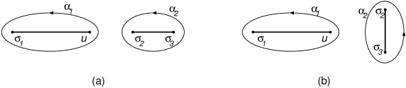
Figure 1: The definition of the $\alpha-$cycles for real positive moduli: (a) $0\leq u\leq\frac{1}{\sqrt{27}}$ and (b) $u>\frac{1}{\sqrt{27}}$.

In the above consideration the moduli were assumed to be nonnegative. To describe negative values of moduli, $u<0$, we use invariance of the curve (3.9) under $x\to-x$ and $u\to-u$. This transformation interchanges the $\alpha-$cycles on the complex $x-$plane and leads to the relation $u(\delta_{1},\delta_{2})=-u(\delta_{2},\delta_{1})$ with $\delta_{1}+\delta_{2}=1$. Therefore, as a function of $\delta\equiv\delta_{1}$ the moduli $u(\delta)\equiv u(\delta,1-\delta)$ satisfies the condition

$$u(1-\delta)=-u(\delta)\,,$$ (3.16)

which maps positive and negative values of $u$.

3.3. Reference points

Before integrating the Whitham equations (3.8) let us consider the quantization conditions (3.3) at three reference points on the moduli space, $u=0$, $u=\frac{1}{\sqrt{27}}$ and $u\to\infty$, and find the corresponding values of the flow parameter $\delta$.

For $u=0$, or equivalently $m=\frac{1}{2}$, we get from (3.3)

$$\delta(0)=\frac{1}{\pi}\oint_{\alpha_{1}}\frac{dx}{\sqrt{1-4x^{2}}}=\frac{2}{\pi}\int_{-1/2}^{0}\frac{dx}{\sqrt{1-4x^{2}}}=\frac{1}{2}\,.$$ (3.17)

The same result can be also deduced from (3.16). The value of moduli, $u(\frac{1}{2})=0$, corresponds to one of the singularities (3.10) of the curve $\Gamma_{3}$, at which two cuts $[\sigma_{1},u]$ and $[\sigma_{2},\sigma_{3}]$ merge as $\sigma_{2}\to u$ (see Fig.1a).

For $u=\frac{1}{\sqrt{27}}$, or equivalently $m=1$, one approaches another singularity (3.10), at which the cycle $\alpha_{2}$ is shrinking into a point. Two branching points merge, $\sigma_{2}=\sigma_{3}=\frac{1}{2\sqrt{3}}$ and the integrand (3.3) develops a pole at $x=\frac{1}{2\sqrt{3}}$. It is compensated however by vanishing numerator leading to

$$\delta{\left({\mbox{$\frac{1}{\sqrt{27}}$}}\right)}=\frac{1}{2\pi}\oint_{\alpha_{1}}\frac{dx}{\sqrt{{\left({x+\frac{1}{\sqrt{3}}}\right)}{\left({\frac{1}{\sqrt{27}}-x}\right)}}}=\frac{1}{\pi}\int_{-\frac{1}{\sqrt{3}}}^{\frac{1}{\sqrt{27}}}\frac{dx}{\sqrt{{\left({x+\frac{1}{\sqrt{3}}}\right)}{\left({\frac{1}{\sqrt{27}}-x}\right)}}}=1\,.$$ (3.18)

Applying the symmetry (3.16) one also finds that $\delta{\left({-\frac{1}{\sqrt{27}}}\right)}=0$.

For $u\to\infty$, or equivalently $\nu\to\sqrt{3}$ in (3.15), one rescales $x\to(u/2)^{1/3}x$ in (3.3) and obtains the following asymptotics

$$\delta(u\to\infty)=\frac{3}{\pi}{\left({\frac{u}{2}}\right)}^{1/3}\oint_{\alpha_{1}}\frac{dx}{\sqrt{1+x^{3}}}=\frac{6}{\pi}{\left({\frac{u}{2}}\right)}^{1/3}\int_{-1}^{\infty}\frac{dx}{\sqrt{1+x^{3}}}=u^{1/3}\frac{2\pi}{\Gamma^{3}{\left({\frac{2}{3}}\right)}}\,,$$ (3.19)

which is valid up to subleading in $u$ terms.

Relations (3.17), (3.18) and (3.19) determine the values of the flow parameter corresponding to two singularities (3.10) on the moduli space and fix its asymptotics at infinity:

$$u(\mbox{$\frac{1}{2}$})=0\,,\qquad u(1)=\frac{1}{\sqrt{27}}\,,\qquad u(\delta)\stackrel{{\scriptstyle\delta\to\infty}}{{=}}\frac{\Gamma^{9}{\left({\frac{2}{3}}\right)}}{(2\pi)^{3}}\delta^{3}\,.$$ (3.20)

Let us now apply the Whitham equations (3.8) to reconstruct the flow $u=u(\delta)$ between these reference points. We shall consider separately two branches, $0\leq u<\frac{1}{\sqrt{27}}$ for $\frac{1}{2}\leq\delta<1$ and $u>\frac{1}{\sqrt{27}}$ for $\delta>1$, and then glue them together at $u=\frac{1}{\sqrt{27}}$.

3.4. Whitham flow for $0\leq u\leq\frac{1}{\sqrt{27}}$

For real positive moduli inside the interval $0\leq u\leq\frac{1}{\sqrt{27}}$ the definition of the $\alpha-$cycles is shown on Fig. 1a. The Whitham equation (3.8) looks like

$$\frac{\partial\delta}{\partial u}=\frac{1}{\pi}\int_{\sigma_{1}}^{u}\frac{dx}{\sqrt{(u-x)(4x^{3}-x+u)}}\,,$$ (3.21)

where $\delta\equiv\delta_{1}$ and the branching point $\sigma_{1}$ takes real values defined in (3.12). The elliptic integral entering the r.h.s. of (3.21) is explicitly positive thus implying that $u$ is an increasing single valued function of $\delta$. It can be expressed in terms of the elliptic function of the 1st kind defined in the Appendix, (A.1), as

$$\frac{\partial\delta}{\partial u}=\frac{{\hbox{{\rm I}\kern-1.99997pt\hbox{\rm K}}}(z)}{\pi\sqrt{c}}\,.$$ (3.22)

Here the following notations were introduced

$$c=\frac{(2-m)^{3}m}{12(m^{2}-m+1)^{2}}\,,\qquad z=\frac{(m+1)^{3}(m-1)}{m(m-2)^{3}}\,,$$ (3.23)

the parameter $m$ was defined in (3.11) and for the moduli inside the interval $0\leq u\leq\frac{1}{\sqrt{27}}$ its value can be restricted as $\frac{1}{2}\leq m\leq 1$.

Relation (3.22) defines the derivative $\frac{\partial\delta}{\partial u}$ as a function of the parameter $m$. Replacing $u$ by its expression (3.13) one integrates (3.22) to obtain the dependence of the moduli on the flow parameter through the parametric dependence $u=u(m)$ and $\delta=\delta(m)$ on the interval $\frac{1}{2}\leq m\leq 1$. In this way, one reconstructs the branch of the curve $u=u(\delta)$ for $0\leq u\leq\frac{1}{\sqrt{27}}$ and $\frac{1}{2}\leq\delta\leq 1$ shown in Fig. 2. However, trying to obtain the explicit form of the function $u=u(\delta)$ by inverting the relations $u=u(m)$ and $\delta=\delta(m)$ one realizes that the parameter $m$ is not a well defined function of the moduli due to invariance of (3.13) under modular transformations of $m$. Additionally, the end points, $m=\frac{1}{2}$ and $m=1$, correspond to the singularities on the moduli space (3.10), $u=0$ and $u=\frac{1}{\sqrt{27}}$, respectively, and one should expect to find a nonanalyticity in the dependence $u=u(\delta)$ at their vicinity.

In order to define a good parameter of the expansion of moduli which will replace $m$ and will allow to study analyticity properties of the function $u=u(\delta)$ one introduces the dual flow parameter $\delta_{D}$. In analogy with (3.3) it is defined as an integral of the Whitham differential $dS_{0}$ on the elliptic curve $\Gamma_{3}$ along the $\beta-$cycle encircling the interval $[u,\sigma_{2}]$

$$\delta_{D}=\frac{1}{\pi}\int_{u}^{\sigma_{2}}\frac{(3u-2x)dx}{\sqrt{(x-u)(4x^{3}-x+u)}}\,.$$

The dependence of the moduli on $\delta_{D}$ is described by the Whitham equation similar to (3.21)

$$\frac{\partial\delta_{D}}{\partial u}=\frac{1}{\pi}\int_{u}^{\sigma_{2}}\frac{dx}{\sqrt{(x-u)(4x^{3}-x+u)}}=\frac{{\hbox{{\rm I}\kern-1.99997pt\hbox{\rm K}}}(1-z)}{\pi\sqrt{c}}$$ (3.24)

with $z$ and $c$ given by (3.23). The flow parameters $\delta$ and $\delta_{D}$ are not independent and their mutual derivative defines the Jacobi $\tau$- and $q-$parameters of the elliptic curve $\Gamma_{3}$

$$q=\mathop{\rm e}\nolimits^{i\pi\tau}\,,\qquad\quad\tau=i\frac{\partial\delta_{D}}{\partial\delta}=i\frac{{\hbox{{\rm I}\kern-1.99997pt\hbox{\rm K}}}(1-z)}{{\hbox{{\rm I}\kern-1.99997pt\hbox{\rm K}}}(z)}\,.$$ (3.25)

In agreement with the Riemann theorem, $\tau$ has a positive definite imaginary part and additionally $\mathop{\rm Re}\nolimits\tau=0$ for real moduli inside the interval $0\leq u\leq\frac{1}{\sqrt{27}}$. This property leads to $0\leq q<1$ and it suggests us to identify the $q-$parameter as a good parameter of the expansion of the solutions, $u=u(q)$ and $\delta=\delta(q)$, of the Baxter equation.

3.4.1. Flow at the vicinity of $u=\frac{1}{\sqrt{27}}$

Let us first develop the $q-$expansion of $u$ at the vicinity of $u=\frac{1}{\sqrt{27}}$. This value corresponds to the parameter $m=1$ in (3.13) and one uses (3.25) and (3.23), combined with the properties of the elliptic function (A.5), to find the leading asymptotics of the elliptic parameters $\tau$ and $q$ as

$$\tau=-\frac{i}{\pi}\ln\frac{1-m}{2}\,,\qquad q=\frac{1-m}{2}\qquad\mbox{as $m\to 1$}\,.$$ (3.26)

Similarly, expanding (3.13), (3.22) and (3.24) near $m=1$ one gets using (A.2)

$$u=\frac{1}{\sqrt{27}}\left[1-\frac{27}{8}(1-m)^{2}\right]\,,\qquad\frac{\partial\delta}{\partial m}=\frac{9}{4}(1-m)\,,\qquad\frac{\partial\delta_{D}}{\partial m}=-\frac{9}{4\pi}(1-m)\ln(1-m)\,,$$

where only leading terms were kept. We conclude from these relations that at the vicinity of $u=\frac{1}{\sqrt{27}}$ the moduli $u$ is an analytical function of the flow parameter $\delta$ and not of the dual parameter $\delta_{D}$.

It follows from (3.26) that the $q-$parameter vanishes at $m=1$ and one can expand $u$ and $\delta$ into a power series in $q$. Indeed, using (3.25), (3.23) and (A.5) to invert the dependence $q=q(m)$ near $m=1$

$$1-m=2q-2q^{2}-2q^{3}+6q^{4}-4q^{5}-6q^{6}+{\cal O}(q^{7})$$

and integrating (3.22), one obtains first few terms of the weak coupling $q-$expansion of the moduli and the flow parameter as

$$u = \frac{1}{\sqrt{27}}\left[1-\frac{27}{2}q^{2}+\frac{891}{8}q^{4}-\frac{12879}{16}q^{6}+\frac{716499}{128}q^{8}-\frac{9730773}{256}q^{10}+{\cal O}(q^{12})\right]$$

$$\delta = 1-\frac{9}{2}q^{2}+\frac{189}{8}q^{4}-\frac{1917}{16}q^{6}+\frac{83421}{128}q^{8}-\frac{929367}{256}q^{10}+{\cal O}(q^{12})\,,$$ (3.27)

where only even powers of $q$ appear. Finally, one inverts the second relation and expresses the moduli as a power series in the flow parameter $\delta$

$$u=\frac{1}{\sqrt{27}}\left[1-3\bar{\delta}+2\bar{\delta}^{2}-\frac{2}{9}\bar{\delta}^{3}+\frac{10}{81}\bar{\delta}^{4}+\frac{38}{243}\bar{\delta}^{5}+{\cal O}(\bar{\delta}^{6})\right]\,,\qquad\bar{\delta}\equiv 1-\delta\,.$$ (3.28)

This expression provides the solution to the Whitham equation (3.21) at the vicinity of $\delta=1$ and $u=\frac{1}{\sqrt{27}}$. One verifies that it coincides with analogous expression first obtained within the class of polynomial solutions of the Baxter equation [10, 14]. Applying (3.16) one can also find the behaviour of the moduli around $\delta=0$.

3.4.2. Flow at the vicinity of $u=0$

The series (3.28) has a finite radius of convergence and for $\delta$ close to $\delta=\frac{1}{2}$ one expects the dependence $u=u(\delta)$ to be drastically changed since the reference point $u(\frac{1}{2})=0$ is another singularity of the curve, (3.10). One finds from (3.13) that $u=0$ corresponds to $m=\frac{1}{2}$ and one calculates the values of the Jacobi parameters of the curve, (3.25), using (3.23) and (A.6), as $\tau=0$ and $q=1$. Thus, to approach the point $u=0$ on the moduli space using (3.27) one has to develop the strong coupling expansion in $q$.

Let us show that at the vicinity of $u=0$ the strong coupling expansion of moduli $u$ in $q=\exp(i\pi\tau)$ is equivalent to the weak coupling expansion in the dual parameter $q_{D}$ defined as

$$q_{D}=\mathop{\rm e}\nolimits^{-\frac{i\pi}{3\tau}}\,,\qquad\quad\ln q\ln q_{D}=\frac{\pi^{2}}{3}\,.$$ (3.29)

Repeating previous analysis we examine the behaviour of $\tau$ and $q_{D}$ near $m=\frac{1}{2}$. One gets using (A.6) and (3.23)

$$\tau=-\frac{i\pi}{3}\frac{1}{\ln\left[\frac{2}{3}(m-\frac{1}{2})\right]}\,,\qquad q_{D}=\frac{2}{3}{\left({m-\frac{1}{2}}\right)}\to 0$$

and observes that $q_{D}$ vanishes at $m=\frac{1}{2}$ while $q=1$. As $m\to\frac{1}{2}$, the expansion of the Whitham equations (3.22) and (3.24) using (A.3) leads to the following relations

$$u=\frac{2}{3}{\left({m-\frac{1}{2}}\right)}\,,\qquad\frac{\partial\delta}{\partial m}=-\frac{2}{\pi}\ln\left[\frac{2}{3}{\left({m-\frac{1}{2}}\right)}\right]\,,\qquad\frac{\partial\delta_{D}}{\partial m}=\frac{2}{3}\left[1-\frac{14}{3}{\left({m-\frac{1}{2}}\right)}^{2}\right]\,.$$

They imply that as a function of the flow parameter $u=u(\delta)$ has a singularity at $\delta=\frac{1}{2}$

$$\delta\sim\frac{1}{2}-\frac{3}{\pi}u\ln u\,,\qquad\mbox{as $u\to 0$}\,,$$ (3.30)

and at the same time $u$ is an analytical function of the dual flow parameter $\delta_{D}$. This suggests to search for the moduli as a function of the dual flow parameter $\delta_{D}$ and identify the dual parameter $q_{D}$ as an appropriate parameter of the perturbative expansion of the moduli around $u=0$.

Using (3.29), (3.25), (3.23) and (A.6) to invert the dependence $q_{D}=q_{D}(m)$ near $m=\frac{1}{2}$

$$m-\frac{1}{2}=\frac{3}{2}q_{D}-3q_{D}^{3}+\frac{9}{2}q_{D}^{5}-6q_{D}^{7}+\frac{21}{2}q_{D}^{9}-18q_{D}^{11}+{\cal O}(q_{D}^{13})$$

and integrating the dual Whitham equation (3.24), one obtains the following relations

$$u = q_{D}-\frac{15}{2}q_{D}^{3}+\frac{459}{8}q_{D}^{5}-\frac{6547}{16}q_{D}^{7}+\frac{339955}{128}q_{D}^{9}+{\cal O}(q_{D}^{11})$$

$$\delta_{D} = q_{D}-\frac{11}{2}q_{D}^{3}+\frac{243}{8}q_{D}^{5}-\frac{2599}{16}q_{D}^{7}+\frac{113699}{128}q_{D}^{9}+{\cal O}(q_{D}^{11})\,,$$ (3.31)

which provide a weak coupling expansion of the moduli and the dual flow parameter in $q_{D}$. Inverting the dependence $\delta_{D}=\delta_{D}(q_{D})$ we obtain from (3.31) the expression for $u=u(\delta_{D})$ as a power series in the dual flow parameter $\delta_{D}$

$$u=\delta_{{D}}-2\,\delta_{{D}}^{3}-6\,\delta_{{D}}^{5}-48\,\delta_{{D}}^{7}-510\,\delta_{{D}}^{9}+{\cal O}\left(\delta_{{D}}^{11}\right)\,,$$

which should be compared with (3.28). Finally, to restore the dependence of the moduli on $\delta$, one rewrites the definitions (3.25) and (3.29) in the form

$$\delta=\frac{1}{2}-\frac{3}{\pi}\int_{0}^{q_{D}}dq_{D}\ln q_{D}\frac{\partial\delta_{D}}{\partial q_{D}}\,.$$

and replaces $\delta_{D}$ by its expression (3.31). This gives the $q_{D}-$expansion of $\delta$ which can be combined with the first relation in (3.31) to determine the nonleading terms in the asymptotic expansion (3.30)

$$\delta\stackrel{{\scriptstyle u\to 0}}{{=}}\frac{1}{2}-\frac{3}{\pi}{\left({u+2u^{3}+18u^{5}}\right)}\ln u+\frac{1}{\pi}{\left({3u-\frac{11}{2}u^{3}-\frac{1323}{20}u^{5}}\right)}+{\cal O}(u^{7})\,.$$ (3.32)

This relation can be inverted and $u$ can be expressed in terms of the Lambert function of $\delta$.

3.5. Whitham flow for $u>\frac{1}{\sqrt{27}}$

The Whitham equation for $u>\frac{1}{\sqrt{27}}$ has the same form as (3.21), but important difference with the previous case is that two branching points, $\sigma_{2}$ and $\sigma_{3}$, take complex values. According to our choice of the cuts between the branching points, shown in Fig. 1b, the elliptic integral entering the r.h.s. of (3.21) takes real positive values defining $u$ to be an increasing single valued function of $\delta$ for $\delta>1$. Since $u=u(\delta)$ has the same property for $0\leq\delta<1$ it can be now extended using (3.16) to arbitrary real $\delta$.

Using parameterization of the branching points (3.14) the elliptic integral in (3.21) can be calculated as

$$\frac{\partial\delta}{\partial u}=\frac{2\sqrt{3}}{\pi}\frac{\nu^{2}-3}{(9+\nu^{2})^{3/4}(1+\nu^{2})^{1/4}}{\hbox{{\rm I}\kern-1.99997pt\hbox{\rm K}}}{\left({\frac{1}{2}-\frac{1}{2}\mathop{\rm Re}\nolimits\left[\frac{(\nu+i)(\nu-3i)^{3}}{(\nu-i)(\nu+3i)^{3}}\right]^{1/2}}\right)}\,,$$ (3.33)

where $\nu\geq\sqrt{3}$. Replacing $u$ by its expression (3.15) one integrates numerically (3.33) to restore the $\nu-$dependence of $\delta$ and then calculates the moduli through the parametric dependence $u=u(\nu)$. This gives the second branch of the curve $u=u(\delta)$ for $\delta>1$ shown in Fig. 2.

To specify the appropriate boundary conditions for (3.33) one considers two values of the parameter: $\nu=\sqrt{3}$ and $\nu\to\infty$. For $\nu\to\sqrt{3}$ one finds from (3.15) that $u$ infinitely increases and its leading asymptotic behaviour in $\delta$ is given by (3.20). For $\nu\to\infty$ one gets from (3.15) and (3.20) the corresponding value of moduli as $u=\frac{1}{\sqrt{27}}$ for $\delta=1$. Let us consider the flow of $u$ in both cases in more detail.

For large $\nu$ one uses (3.15) and (3.33) to expand $u$ and $\delta$ in inverse powers of $1/\nu$

$$u = \frac{1}{\sqrt{27}}\left(1+{\frac{27}{2}}\,{\nu}^{-2}+{\frac{459}{8}}\,{\nu}^{-4}+{\frac{3375}{16}}\,{\nu}^{-6}+{\frac{93555}{128}}\,{\nu}^{-8}+{\frac{627669}{256}}\,{\nu}^{-10}+{\cal O}({\nu}^{-12})\right)$$

$$\delta = 1+\frac{9}{2}\,{\nu}^{-2}+{\frac{45}{8}}\,{\nu}^{-4}+{\frac{477}{16}}\,{\nu}^{-6}+{\frac{189}{128}}\,{\nu}^{-8}+{\frac{110295}{256}}\,{\nu}^{-10}+{\cal O}({\nu}^{-12})\,.$$

Inverting these relations one obtains the expansion of $u$ in powers of $\bar{\delta}=1-\delta$, which identically coincides with (3.28). This means that two different branches of the function $u(\delta)$ corresponding to the Whitham flow for $\frac{1}{2}\leq\delta<1$ and $\delta>1$ can be smoothly glued at $\delta=1$ (see Fig. 2).

For $\nu\to\sqrt{3}$ the moduli (3.15) goes to infinity as

$$u=4(\nu^{2}-3)^{-3/2}+(\nu^{2}-3)^{-1/2}+{\cal O}{\left({(\nu^{2}-3)^{3/2}}\right)}\,.$$ (3.34)

To find the corresponding behaviour of the flow parameter one takes into account that $\delta=1$ for $\nu=\infty$ and integrates the Whitham equation (3.33) as

$$\delta=1+\int_{\infty}^{\nu}d\nu\,\frac{\partial u}{\partial\nu}\,\frac{\partial\delta}{\partial u}\,.$$

Replacing the derivative $\frac{\partial\delta}{\partial u}$ by its expression (3.33), we expand the integral around $\nu^{2}=3$ and apply (A.4) to get after some calculations

$$\delta=\frac{2^{5/3}\pi}{\Gamma^{3}{\left({\frac{2}{3}}\right)}}\ (\nu^{2}-3)^{-1/2}-1+{\cal O}{\left({(\nu^{2}-3)^{1/2}}\right)}\,.$$ (3.35)

Combining together (3.34) and (3.35) we obtain the asymptotic behaviour of the moduli at large positive values of the flow parameter $\delta$

$$u=\frac{\Gamma^{9}{\left({\frac{2}{3}}\right)}}{(2\pi)^{3}}\,{\left({\delta^{3}+3\delta^{2}}\right)}\times\left[1+{\cal O}(1/\delta)\right]\,,\qquad\mbox{as $\delta\to\infty$}\,.$$ (3.36)

Here, the leading term coincides with (3.20). The symmetry (3.16) allows to extend the flow to large negative $u$ as

$$u=\frac{\Gamma^{9}{\left({\frac{2}{3}}\right)}}{(2\pi)^{3}}\,{\left({\delta^{3}-6\delta^{2}}\right)}\times\left[1+{\cal O}(1/\delta)\right]\,,\qquad\mbox{as $\delta\to-\infty$}\,.$$ (3.37)

Figure 2: Quantized moduli $u$ for real values of the flow parameter $\delta$. The dots indicate the positions of three singularities of the elliptic curve $\Gamma_{3}$ located at $\delta-\frac{1}{2}=\pm\frac{1}{2}$ and $0$. The behaviour of the function $u=u(\delta)$ around these points and at infinity is described by (3.32), (3.28) and (3.36).

Summarizing the results of this Section we present on Fig. 2 the dependence of the quantized moduli $u=u(\delta)$ on the flow parameter $-\infty<\delta<\infty$. According to (3.16) the moduli $u$ is an odd function of $\delta-\frac{1}{2}$. Its asymptotics around $\delta=1/2$, $1$ and $\infty$ is described by (3.32), (3.28) and (3.36), respectively. We recall that this curve provides the solution to the quantization conditions (3.3) and (3.8) for $N=3$ reggeon compound states.

4. Quantum numbers of $N=3$ reggeon states

Let us apply the results of the previous section to evaluate the quantum numbers $q_{2}$ and $q_{3}$ of the $N=3$ reggeon states in the leading order of the WKB expansion. According to (2.25), the values of $q_{3}$ depend on two complex numbers $\ell_{1}=\frac{n_{1}}{2}+i\nu_{1}$ and $\ell_{2}=\frac{n_{2}}{2}+i\nu_{2}$. Following (3.4) and (3.5) we consider two special cases, $n_{1}=n_{2}=0$ and $\nu_{1}=\nu_{2}=0$, corresponding to real values of the moduli and the flow parameters. In the case I, the relations (3.4) and (3.6) between the moduli and quantized $q_{3}$ can be written in two equivalent forms

$$q_{3}=(i\nu)^{3}\times u{\left({\frac{\nu_{1}}{\nu}}\right)}\,,\qquad\quad h-\frac{1}{2}=i\nu\,,\qquad\quad\nu=\nu_{1}+\nu_{2}$$ (4.1)

or

$$q_{3}=(i\nu_{1})^{3}\times u(\delta)\,\delta^{-3}\,,\qquad\quad h-\frac{1}{2}=(i\nu_{1})\times\delta^{-1}\,,\qquad\quad\delta=\frac{\nu_{1}}{\nu_{1}+\nu_{2}}\,,$$ (4.2)

with $\nu_{1,2}$ being real. In the case II, one gets similar relations by replacing $i\nu_{k}\to\frac{1}{2}n_{k}$ and taking $n_{1,2}$ to be integer.

It is easy to see from (3.16) that $q_{3}$ is antisymmetric under interchanging of $\nu_{1}$ and $\nu_{2}$, while the conformal weight $h=\frac{1}{2}+i(\nu_{1}+\nu_{2})$ is explicitly symmetric. Therefore, $q_{3}$ vanishes for $\nu_{1}=\nu_{2}$ and the corresponding $N=3$ reggeon state with the conformal weight $h=\frac{1}{2}+2i\nu_{1}$ is degenerate [9]. Their wave function does not depend on one of the reggeon coordinates and the corresponding energy is equal to the energy of $N=2$ reggeon state, $E_{3}(q_{3}=0,h)=E_{2}(h)$.

Since quantized $q_{3}$ and $h$ depend on the same parameters $\nu_{1}$ and $\nu_{2}$ one can express $\nu_{2}$ in terms of $h$ and consider $q_{3}$ to be a function of the conformal weight $h$ and real $\nu_{1}$. Let us consider separately the dependence of $q_{3}$ on its arguments, $q_{3}=q_{3}(h,\nu_{1})$.

For fixed values of the conformal weight $h={\rm fixed}$ it is convenient to apply (4.1). One finds that up to rescaling of the argument the $\nu_{1}-$dependence of $q_{3}$ is governed by the moduli and it follows the pattern of the curve shown in Fig. 2.

For fixed values of $\nu_{1}$ one uses instead (4.2). Introducing notations for $q=u(\delta)\,\delta^{-3}$ and $x=\delta^{-1}$ one writes (4.2) as

$$q_{3}=(i\nu_{1})^{3}\times q(x)\,,\qquad\quad h-\frac{1}{2}=i\nu_{1}\times x\,,\qquad\quad q=x^{3}u(1/x)\,,$$ (4.3)

with $q$ depending on $x$ and not on $\nu_{1}$. Here, the parameter $\nu_{1}$ fixes the scale of $q_{3}$ and $h-\frac{1}{2}$. It takes real continuous values which cannot be however arbitrary small for the leading order WKB approximation to be applicable. In the case II one replaces $i\nu_{1}\to\frac{1}{2}n_{1}$ and uses integer $n_{1}$ to label the curves $q_{3}=q_{3}(h;n_{1})$. Again, the values of $n_{1}$ cannot be small.

The function $q=q(x)$ can be determined out of the curve $u=u(\delta)$ depicted on Fig. 2 in two steps. One first finds the dependence of moduli $u$ on $x=1/\delta$ as shown in Fig. 3 and then obtains $q=q(x)$ in the form shown in Fig. 4.

Figure 3: Two different branches of the function $u(1/x)$ entering into (4.3). Dotted lines represent $u=\pm\frac{1}{\sqrt{27}}$ and two dots indicate the singular points $x=1$, $u=\frac{1}{\sqrt{27}}$ and $x=2$, $u=0$. The part of the curve $u^{2}(x)\leq\frac{1}{27}$ corresponds to the polynomial solutions of the Baxter equation and it should be compared with Fig. 4 in [10].

The following comments are in order. To describe the transition from Fig. 2 to Fig. 3 one has to take into account that $\delta=0$ is mapped into infinities $x=\pm\infty$ and two parts of the continuous function $u=u(\delta)$ for $\delta<0$ and $\delta>0$ give rise to two branches of the functions $u$ and $q$ on Figs. 3 and 4, respectively.

Figure 4: The function $q=q(x)$ defining the quantum numbers (4.3) of the $N=3$ reggeon compound states. Its behaviour around $x=0_{\pm}$, $x=1$, $x=2$ and $x=\pm\infty$ is given by (4.5), (4.6), (4.8), (4.7) and (4.4), respectively.

The asymptotics of $q$ as $x\to\pm\infty$ follows from (3.28) and (3.16)

$$q=-\frac{x^{3}}{\sqrt{27}}\left[1-\frac{3}{x}+{\cal O}{\left({\frac{1}{x^{2}}}\right)}\right]\,,\quad\mbox{as $x\to\pm\infty$}\,.$$ (4.4)

Two infinities $\delta\to\pm\infty$ are mapped into the origin $x=0$. Since $u=u(\delta)$ has different subleading terms in the asymptotics (3.36) and (3.37), the function $q$ has different asymptotics as $x$ approaches the origin from different sides (see Fig. 4)

$$q=\frac{\Gamma^{9}(2/3)}{(2\pi)^{3}}\left[1+3x+{\cal O}(x^{2})\right]\,,\qquad\mbox{as $x\to 0_{+}$}$$ (4.5)

and

$$q=\frac{\Gamma^{9}(2/3)}{(2\pi)^{3}}\left[1-6x+{\cal O}(x^{2})\right]\,,\qquad\mbox{as $x\to 0_{-}$}$$ (4.6)

It is this property that is responsible for the appearance of a cusp on Fig. 4 at $x=0$ and $q=\frac{\Gamma^{9}(2/3)}{(2\pi)^{3}}=0.0617...$ Two reference points (3.17) and (3.18) correspond to $x=2$ and $x=1$, respectively, and the asymptotics of $q$ at their vicinity can be found from (3.30) and (3.28) as

$$q\ln q=\frac{2\pi}{3}{\left({x-2}\right)}\,,\quad\mbox{as $x\to 2$}$$ (4.7)

and

$$q=\frac{1}{\sqrt{27}}\left[1-(x-1)^{2}+{\cal O}{\left({(x-1)^{3}}\right)}\right]\,,\quad\mbox{as $x\to 1$}\,.$$ (4.8)

The part of the function $u=u(\delta)$ corresponding to $0\leq\delta\leq 1$ and $u^{2}\leq\frac{1}{27}$ describes the polynomial solutions of the Baxter equation. It is mapped into the branch that starts at $q=\frac{1}{\sqrt{27}}$ for $x=1$ on Fig. 4 and then decreases to infinity according to (4.4) as $x$ increases. One checks that this behaviour is an agreement with the numerical results (see Fig. 4 in [10]).

We would like to stress that the above results were obtained in the leading order of the WKB expansion and they are valid for large values of quantum numbers. Examining Fig. 4 and using (4.3) one notices that the latter condition is violated at $x=0$ and $x=2$ when either $|h-\frac{1}{2}|$ or $q_{3}$ vanish. Therefore, one should expect that the behaviour of the function $q=q(x)$ close to the cusp on Fig. 4 and around the point $q=0$ will be modified by the nonleading WKB corrections. Their detailed analysis deserves further investigation.

Figure 5: The energy spectrum of the $N=3$ reggeon compound states evaluated in the leading order of the WKB quantization for type-II quantization conditions, $E_{3}=E_{3}(h;n_{1})$. Three different curves correspond to $n_{1}=4$, $8$ and $12$. The dotted line represents the BFKL energy of the $N=2$ reggeon state, $E_{2}(h)=4\left[{\Psi(1)-\Psi(\frac{1}{2}+|h-\frac{1}{2}|)}\right]$.

Concluding our consideration we would like to apply the obtained results to calculate the energy of the $N=3-$reggeon states. The corresponding expression looks like

$$E_{3}^{\rm WKB}(q_{2},q_{3})=-2\ln 2-\sum_{j=1}^{3}\left[\Psi(1+i\delta_{j})+\Psi(1-i\delta_{j})-2\Psi(1)\right]$$ (4.9)

where $\Psi(x)=\frac{d}{dx}\ln\Gamma(x)$ and $\delta_{j}$ are defined as zeros of $\Lambda(x)$

$$\Lambda(\delta_{j})=2\delta_{j}^{3}+q_{2}\delta_{j}+q_{3}=0\,.$$

One should warn however that, first, this expression was obtained for the type-II solutions (3.5) and, second, it is not exact and is valid in the leading order of the WKB expansion. Replacing $i\nu_{1}\to n_{1}/2$ in (4.3) and substituting quantized $q_{2}$ and $h$ into (4.9) one gets $E_{3}=E_{3}(h;n_{1})$ as a function of the conformal weight $h$ and integer $n_{1}$. To get an insight into the spectrum of $E_{3}$ we plot on Fig. 5 the dependence of $E_{3}$ on the conformal weight $h$ for different values of the integer $n_{1}$. These curves are in an agreement with the numerical results of the polynomial solutions (see Fig. 8 in [10]) and they support the calculation of the odderon intercept performed in [10]. For given $n_{1}$ the energy is maximal for $h=\frac{1}{2}$ and its value increases as $n_{1}$ decreases. The absolute maximum of the energy $E_{0}={\rm max}_{h,n_{1}}E_{3}(h;n_{1})$ defines the odderon intercept and it is expecting to occur at $n_{1}=1$ and $h=\frac{1}{2}$. One also observes that for the upper curve on Fig. 5 the maximal energy, $E_{3}(\frac{1}{2};4)<E_{0}$, is close to the lower bound on the odderon energy obtained in the variational approach [24]. We refer to [10] for detailed description of the properties of curves shown on Fig. 5. It would be interesting to improve (4.9) by applying the expression for the energy $E_{3}$ proposed in [11].

5. Summary

In this paper, we have studied the spectrum of the reggeon compound states in high-energy QCD. These states appear as solutions of the $(2+1)-$dimensional Schrödinger equation (1.1) which exhibits remarkable properties of the $SL(2,\hbox{$\,\vrule height=6.45831pt,width=0.4pt,depth=0.0pt\kern-3.00003pt{\rm C}$})$ invariance and complete integrability. As a result, the energy of the states can be evaluated as a function of the set of quantum numbers $q_{2}$, $...$, $q_{N}$. The latter are defined as eigenvalues of the mutually commuting integrals of motions and their possible values are constrained by the quantization conditions.

We have established the quantization conditions by applying the methods of nonlinear WKB analysis to the $N-$reggeon Schrödinger equation in the separated coordinates. In the leading order of the WKB expansion, the $N$ reggeon state looks like the classical system of $N$ particles moving on the $2-$dimensional plane of transverse gluon coordinates along periodic trajectories. This collective motion can be also considered as a propagation of the soliton wave in the system of $N$ reggeons. The charges $q_{2}$, $...$, $q_{N}$ become parameters of the soliton waves.

The quantization conditions follow from the analysis of the wave function of the $N$ reggeon state in the leading order of the WKB expansion. Requiring the wave function to be a single-valued function of the separated coordinates, we have found that the selection rules for $q_{2}$, $...$, $q_{N}$ have the form of the Bohr-Sommerfeld quantization conditions imposed on the reggeon classical trajectories in the action-angle variables. The same conditions can be interpreted as Whitham equations on the moduli of the spectral curve $\Gamma_{N}$ corresponding to the classical $N$ reggeon system. We have solved the Whitham equation for $N=3$ reggeon states by using the properties of the elliptic integrals on the curve $\Gamma_{3}$. The quantized $q_{2}$ and $q_{3}$ were obtained in the form of perturbative expansion in powers of the Jacobi $q-$parameter of the elliptic curve $\Gamma_{3}$. Different parts of the spectrum of $q_{2}$ and $q_{3}$ correspond to the weak, $q\ll 1$, and strong, $q\sim 1$, coupling regime of the perturbative $q-$series. In the latter case, one performs the duality transformation to express $q_{2}$ and $q_{3}$ as a weak coupling expansion in the dual coupling constant, $q_{D}\ll 1$. Combining together different branches we have obtained the spectrum of quantized $q_{2}$ and $q_{3}$ which is in agreement with available exact solutions found within algebraic Bethe Ansatz approach.

In conclusion, one should mention that the above consideration was restricted to the leading order WKB expansion and one should additionally study the importance of nonleading corrections. In particular, considering the behaviour of (2.10) around the origin $x=0$ one can argue [10] that nonleading WKB corrections to $Q(x)$ become equally important. As in the case of the polynomial solutions, (2.9), the analysis of the singularities of the solutions to the Baxter equation at $x=0$ should lead to additional constaints on the quantum numbers of the reggeon states and presumably fix the ratio $C_{+-}/C_{-+}$ in (2.8). These questions deserve additional studies.

Appendix: Elliptic integral of the first kind

In this appendix we collect some useful properties of the elliptic integral of the first kind. It is defined as [22, 23]

$${\hbox{{\rm I}\kern-1.99997pt\hbox{\rm K}}}(z)=\int_{0}^{1}\frac{dx}{\sqrt{(1-x^{2})(1-zx^{2})}}=\frac{\pi}{2}F{\left({\mbox{$\frac{1}{2}$,$\frac{1}{2}$};1;z}\right)}$$ (A.1)

with $F$ being a hypergeometric function. For $z\to 0$ it behaves as

$${\hbox{{\rm I}\kern-1.99997pt\hbox{\rm K}}}(z)=\frac{\pi}{2}\left\{1+{\left({\frac{1}{2}}\right)}^{2}z+{\left({\frac{1\cdot 3}{2\cdot 4}}\right)}^{2}z^{2}+...\right\}$$ (A.2)

and for $z\to 1$ as

$${\hbox{{\rm I}\kern-1.99997pt\hbox{\rm K}}}(z)=-\frac{1}{\pi}{\hbox{{\rm I}\kern-1.99997pt\hbox{\rm K}}}(1-z)\,\ln\frac{1-z}{16}-2\mbox{${\left({\frac{1}{2}}\right)}^{2}\frac{1}{1\cdot 2}$}(1-z)-2\mbox{${\left({\frac{1\cdot 3}{2\cdot 4}}\right)}^{2}{\left({\frac{1}{1\cdot 2}+\frac{1}{3\cdot 4}}\right)}$}(1-z)^{2}+...$$ (A.3)

Calculating (3.35) one uses the relation

$${\hbox{{\rm I}\kern-1.99997pt\hbox{\rm K}}}{\left({\frac{1}{2}+\frac{\sqrt{3}}{4}}\right)}=\frac{3^{-3/4}2^{2/3}\pi^{2}}{\Gamma^{3}(\frac{2}{3})}\,.$$ (A.4)

The Jacobi $\tau$ and $q$ parameters defined in (3.25) have the following asymptotics for $z\to 0$

$$\tau(z) = \frac{i}{\pi}\ln\frac{16}{z}-\frac{i}{2\pi}{\left({z+{\frac{13}{32}}{z}^{2}+{\frac{23}{96}}{z}^{3}+{\frac{2701}{16384}}{z}^{4}+{\cal O}(z^{5})}\right)}$$

$$q(z) = \frac{x}{16}{\left({1+\frac{1}{2}z+\frac{21}{64}z^{2}+\frac{31}{128}z^{3}+\frac{6257}{32768}z^{4}+{\cal O}(z^{5})}\right)}\,.$$ (A.5)

and their asymptotics for $z\to 1$ can be found using the relations

$$\tau(z)=-\frac{1}{\tau(1-z)}\,,\qquad\quad q(z)=\exp{\left({\frac{\pi^{2}}{\ln q(1-z)}}\right)}\,,$$ (A.6)

which follow from the definition (3.25).

References

-
[1]
J. Bartels, Nucl. Phys. B175 (1980) 365;
J. Kwiecinski and M. Praszalowicz, Phys. Lett. B94 (1980) 413. - [2] L.N. Lipatov, Pomeron in quantum chromodynamic, in “Perturbative QCD”, pp.411–489, ed. A.H. Mueller, World Scientific, Singapore, 1989.
-
[3]
I.M. Gelfand, M.I. Graev and N.Ya. Vilenkin, Generalized
functions, Vol. 5, Academic Press, 1966;
D.P. Zhelobenko and A.I. Shtern, Representations of Lie groups (in Russian), Nauka, Moscow, 1983, pp.211-220. - [4] L.N. Lipatov, Phys. Lett. B251 (1990) 284; B309 (1993) 394.
- [5] L.D. Faddeev and G.P. Korchemsky, [hep-ph/9404173]; Phys. Lett. B 342 (1995) 311.
- [6] L.N. Lipatov, JETP Lett. 59 (1994) 596.
- [7] E.K. Sklyanin, The quantum Toda chain, Lecture Notes in Physics, vol. 226, Springer, 1985, pp.196–233; Functional Bethe ansatz, in “Integrable and superintegrable systems”, ed. B.A. Kupershmidt, World Scientific, 1990, pp.8–33; Progr. Theor. Phys. Suppl. 118 (1995) 35 [solv-int/9504001].
-
[8]
I.V. Komarov and V.V. Zalipaev, J. Phys. A: Math. Gen. 17 (1984) 1479;
I.V. Komarov and V.B. Kuznetsov, J. Phys. A: Math. Gen. 23 (1990) 841. - [9] G.P. Korchemsky, Nucl. Phys. B443 (1995) 255.
- [10] G.P. Korchemsky, Nucl. Phys. B462 (1996) 333.
- [11] J. Wosiek and R.A. Janik, Phys. Rev. Lett. 79 (1997) 2935; in Proceedings of the ICHEP 96, pp.615-618 [hep-th/9611025].
- [12] G.P. Korchemsky, preprint LPTHE-Orsay-97-62 [hep-ph/9711277].
- [13] J. Teschner, preprints LPM-97 [hep-th/9712258]; [hep-th/9712256].
- [14] G.P. Korchemsky, Nucl. Phys. B498 (1997) 68; in Proceedings of the ICHEP 96, pp.713-716 [hep-ph/9610454].
- [15] Z. Maassarani and S. Wallon, J. Phys. A: Math. Gen. 28 (1995) 6423.
- [16] R. A. Janik, Acta Phys. Polon. B27 (1996) 1275.
-
[17]
S.P. Novikov, Func. Anal. Appl. 24 (1990) 296;
I.M. Krichever, ETH preprint, Zürich, June 1990;
G. Moore, Comm. Math. Phys. 133 (1990) 261;
F. Fucito, A. Gamba, M. Martinelli and O. Ragnisco, Int. J. Mod. Phys. B6 (1992) 2123. - [18] V. Pasquier and M. Gaudin, J. Phys. A25 (1992) 5243.
-
[19]
S.P. Novikov, S.V. Manakov, L.P. Pitaevskii and V.E. Zakharov,
Theory of Solitons: The Inverse Scattering Method,
Consultants Bureau, New York, 1984;
B. Dubrovin, I. Krichever and S. Novikov, Integrable systems - I, Sovremennye problemy matematiki (VINITI), Dynamical systems - 4 (1985) 179;
B.A. Dubrovin, V.B. Matveev and S.P. Novikov, Russ. Math. Surv. 31 (1976) 59. - [20] G.P. Korchemsky and I.M. Krichever, Nucl. Phys. B505 (1997) 387.
-
[21]
G.B. Whitham, Linear and Nonlinear Waves,
John Wiley, New York, 1974;
H. Flaschka, M.G. Forest and D.W. McLaughlin, Comm. Pure Appl. Math. 33 (1980) 739;
S.Yu. Dobrokhotov and V.P. Maslov, J. Sov. Math. 16 (1981) 1433;
B.A. Dubrovin and S.P. Novikov, Russ. Math. Surv. 44 (1989) 35.
I.M. Krichever, Comm. Math. Phys. 143 (1992) 415; Comm. Pure Appl. Math. 47 (1994) 437;
B.A. Dubrovin, Comm. Math. Phys. 145 (1992) 195. - [22] Handbook of Mathematical Functions, eds. H. Abramowitz and I. Stegun, Dover, New York, 1972.
- [23] Higher transcendental functions, ed. A. Erdélyi, McGraw-Hill, 1953.
- [24] M.A. Braun, preprint SPbU-IP-1998/3 [hep-ph/9801352].