LAL 97-85
hep-ph/9711308
November 1997

IMPROVED DETERMINATION OF $\alpha(M_{\rm Z}^{2}$) AND THE
ANOMALOUS MAGNETIC MOMENT OF THE MUON
Michel Davier and Andreas Höcker
^bLaboratoire de l’Accélérateur Linéaire,
IN2P3-CNRS et Université de Paris-Sud, F-91405 Orsay, France

Abstract

We reevaluate the hadronic contribution to the running of the QED fine structure constant $\alpha(s)$ at $s=M_{\rm Z}^{2}$. We use data from $e^{+}e^{-}$ annihilation and $\tau$ decays at low energy and at the $q\bar{q}$ thresholds, where resonances occur. Using so-called spectral moments and the Operator Product Expansion (OPE), it is shown that a reliable theoretical prediction of the hadronic production rate $R(s)$ is available at relatively low energies. Its application improves significantly the precision on the hadronic vacuum polarization contribution. We obtain $\Delta\alpha_{\rm had}(M_{\rm Z}^{2})$ $=(277.8\pm 2.6)\times 10^{-4}$ yielding $\alpha^{-1}(M_{\rm Z}^{2})=128.923\pm 0.036$. Inserting this value in a global electroweak fit using current experimental input, we constrain the mass of the Standard Model Higgs boson to be $M_{\rm Higgs}=129^{+103}_{-62}~{}{\rm GeV}$. Analogously, we improve the precision of the hadronic contribution to the anomalous magnetic moment of the muon for which we obtain $a_{\mu}^{\rm had}=(695.1\pm 7.5)\times 10^{-10}$.

(Submitted to Physics Letters B)

.

1 Introduction

The running of the QED fine structure constant $\alpha(s)$ and the anomalous magnetic moment of the muon are famous observables whose theoretical precisions are limited by second order loop effects from hadronic vacuum polarization. Both magnitudes are related via dispersion relations to the hadronic production rate in $e^{+}e^{-}$ annihilation,

$$R(s)=\frac{\sigma_{\rm tot}(e^{+}e^{-}\!\rightarrow{\rm hadrons})}{\sigma_{0}(e^{+}e^{-}\!\rightarrow\mu^{+}\mu^{-})}=\frac{3s}{4\pi\alpha^{2}}\sigma_{\rm tot}(e^{+}e^{-}\!\rightarrow{\rm hadrons})~{}.$$ (1)

While far from quark thresholds and at sufficiently high energy $\sqrt{s}$, $R(s)$ can be predicted by perturbative QCD, theory may fail when resonances occur, i.e., local quark-hadron duality is broken. Fortunately, one can circumvent this drawback by using $e^{+}e^{-}$ annihilation data of $R(s)$ and, as recently proposed in Ref. [1], hadronic $\tau$ decays benefitting from the largely conserved vector current (CVC).
There is a strong interest in the electroweak phenomenology to reduce the uncertainty in $\alpha(M_{\rm Z}^{2})$ which at present is a serious limit to further progress in the determination of the Higgs mass from radiative corrections in the Standard Model. The most constraining observable so far has been ${\rm sin}^{2}\Theta_{W}$ obtained from leptonic asymmetries at the Z pole with an achieved precision of $(\Delta{\rm sin}^{2}\Theta_{W})_{\rm exp}=0.00022$ [2]. The uncertainty from the currently used $\alpha(M_{\rm Z}^{2})$ value translates into $(\Delta{\rm sin}^{2}\Theta_{W})_{\alpha}=0.00023$ [3], justifying the present work.
In this paper, we extend the use of the theoretical QCD prediction of $R(s)$ to energies down to 1.8 GeV. The reliability of this approach is justified by applying the Wilson Operator Product Expansion (OPE) [4] (also called SVZ approach [5]) and fitting the dominant nonperturbative power terms directly to the data by means of spectral moments. An analogous approach has been successfully applied to the theoretical prediction of the $\tau$ hadronic width, $R_{\tau}$, at $M_{\tau}\simeq 1.8~{}{\rm GeV}$ in order to measure the strong coupling constant $\alpha_{s}(M_{\tau}^{2})$ [6, 7, 8, 9].
The paper is organized as follows: first a brief overview over the formulae used is given, then the spectral moments are defined and evaluated experimentally, and the corresponding theoretical evaluation is fitted. On this basis, theoretical predictions of the hadronic vacuum polarization contribution to the running of $\alpha(M_{\rm Z}^{2})$ and to the anomalous magnetic moment of the muon, $(g-2)_{\mu}$, from various energy regimes are determined and, with the addition of experimental data, final values for $\alpha(M_{\rm Z}^{2})$ and $a_{\mu}\equiv(g-2)_{\mu}/2$ are determined.

2 Running of the QED Fine Structure Constant

The running of the electromagnetic fine structure constant $\alpha(s)$ is governed by the renormalized vacuum polarization function, $\Pi_{\gamma}(s)$. For the spin 1 photon, $\Pi_{\gamma}(s)$ is given by the Fourier transform of the time-ordered product of the electromagnetic currents $j_{\rm em}^{\mu}(s)$ in the vacuum $(q^{\mu}q^{\nu}-q^{2}g^{\mu\nu})\,\Pi_{\gamma}(q^{2})=i\int d^{4}x\,e^{iqx}\langle 0|T(j_{\rm em}^{\mu}(x)j_{\rm em}^{\nu}(0))|0\rangle$. With $\Delta\alpha(s)-4\pi\alpha\,{\rm Re}\left[\Pi_{\gamma}(s)-\Pi_{\gamma}(0)\right]$, one has

$$\alpha(s)\>=\>\frac{\alpha(0)}{1-\Delta\alpha(s)}~{},$$ (2)

where $4\pi\alpha(0)$ is the square of the electron charge in the long-wavelength Thomson limit. The contribution $\Delta\alpha(s)$ can naturally be subdivided in a leptonic and a hadronic part.
The leading order leptonic contribution is given by

$$\Delta\alpha_{\rm lep}(M_{\rm Z}^{2})=\frac{\alpha(0)}{3\pi}\sum_{\ell}\left[{\rm ln}\frac{M_{\rm Z}^{2}}{m_{\ell}^{2}}-\frac{5}{3}+{\cal O}\left(\frac{m_{\ell}^{2}}{M_{\rm Z}^{2}}\right)\right]\>=\>314.2\times 10^{-4}~{}.$$ (3)

Using analyticity and unitarity, the dispersion integral for the contribution from the light quark hadronic vacuum polarization $\Delta\alpha_{\rm had}(M_{\rm Z}^{2})$ reads [10]

$$\Delta\alpha_{\rm had}(M_{\rm Z}^{2})\>=\>-\frac{M_{\rm Z}^{2}}{4\pi^{2}\,\alpha}\,{\rm Re}\int\limits_{4m_{\pi}^{2}}^{\infty}ds\,\frac{\sigma_{\rm had}(s)}{s-M_{\rm Z}^{2}-i\epsilon}~{},$$ (4)

where $\sigma_{\rm had}(s)=16\pi^{2}\alpha^{2}(s)/s\cdot{\rm Im}\Pi_{\gamma}(s)$ is given by the optical theorem, and Im$\Pi_{\gamma}$ stands for the absorptive part of the hadronic vacuum polarization correlator. Through Eq. (1), the above dispersion relation can be expressed as a function of $R(s)$:

$$\Delta\alpha_{\rm had}(M_{\rm Z}^{2})\>=\>-\frac{\pi\alpha M_{\rm Z}^{2}}{3}\,{\rm Re}\int\limits_{4m_{\pi}^{2}}^{\infty}ds\,\frac{R(s)}{s(s-M_{\rm Z}^{2})-i\epsilon}~{}.$$ (5)

Employing the identity $1/(x^{\prime}-x-i\epsilon)_{\epsilon\rightarrow 0}={\rm P}\{1/(x^{\prime}-x)\}+i\pi\delta(x^{\prime}-x)$, the integrals (4) and (5) are evaluated using the principle value integration technique.

3 Muon Magnetic Anomaly

It is convenient to separate the prediction $a_{\mu}^{\mathrm{S}M}$ from the Standard Model into its different contributions

$$a_{\mu}^{\mathrm{S}M}\>=\>a_{\mu}^{\mathrm{Q}ED}+a_{\mu}^{\mathrm{h}ad}+a_{\mu}^{\mathrm{w}eak}~{},$$ (6)

where $a_{\mu}^{\mathrm{Q}ED}=(11\,658\,470.6\,\pm\,0.2)\times 10^{-10}$ is the pure electromagnetic contribution (see [11] and references therein), $a_{\mu}^{\rm had}$ is the contribution from hadronic vacuum polarization, and $a_{\mu}^{\mathrm{w}eak}=(15.1\,\pm\,0.4)\times 10^{-10}$ [11, 12, 13] accounts for corrections due to the exchange of the weak interacting bosons up to two loops.
Equivalently to $\Delta\alpha_{\rm had}(M_{\rm Z}^{2})$, by virtue of the analyticity of the vacuum polarization correlator, the contribution of the hadronic vacuum polarization to $a_{\mu}$ can be calculated via the dispersion integral [14]

$$a_{\mu}^{\mathrm{h}ad}\>=\>\frac{\alpha^{2}(0)}{3\pi^{3}}\int\limits_{4m_{\pi}^{2}}^{\infty}ds\,\frac{R(s)\,K(s)}{s}~{}.$$ (7)

Here $K(s)$ denotes the QED kernel [15]

$$K(s)\>=\>x^{2}\left(1-\frac{x^{2}}{2}\right)\,+\,(1+x)^{2}\left(1+\frac{1}{x^{2}}\right)\left({\mathrm{l}n}(1+x)-x+\frac{x^{2}}{2}\right)\,+\,\frac{(1+x)}{(1-x)}x^{2}\,{\mathrm{l}n}x$$ (8)

with $x=(1-\beta_{\mu})/(1+\beta_{\mu})$ and $\beta=(1-4m_{\mu}^{2}/s)^{1/2}$. The function $K(s)$ decreases monotonically with increasing $s$. It gives a strong weight to the low energy part of the integral (4). About 91$\%$ of the total contribution to $a_{\mu}^{\rm had}$ is accumulated at c.m. energies $\sqrt{s}$ below 2.1 GeV while 72$\%$ of $a_{\mu}^{\rm had}$ is covered by the two-pion final state which is dominated by the $\rho(770)$ resonance. Data from vector hadronic $\tau$ decays published by the ALEPH Collaboration provide a very precise spectrum of the two-pion final state as well as new input for the lesser known four-pion final states. This new information improves significantly the precision of the $a_{\mu}^{\rm had}$ determination [1].

4 Theoretical Prediction of $R(s)$

The optical theorem relates the total hadronic width at a given energy-squared $s_{0}$ to the absorptive part of the photon vacuum polarization correlator

$$R(s_{0})=12\pi{\rm Im}\Pi(s_{0}+i\epsilon)~{}.$$ (9)

Perturbative QCD predictions up to next-to-next-to leading order $\alpha_{s}^{3}$ are available for the Adler $D$-function [16] which is the logarithmic derivative of the correlator $\Pi$, carrying all physical information:

$$D(s)=-12\pi^{2}s\frac{d\Pi(s)}{ds}~{}.$$ (10)

This yields the relation

$$R(s_{0})=\frac{1}{2\pi i}\oint\limits_{|s|=s_{0}}\frac{ds}{s}D(s)~{},$$ (11)

where the contour integral runs counter-clockwise around the circle from $s=s_{0}-i\epsilon$ to $s=s_{0}+i\epsilon$. Choosing the renormalization scale to be the physical scale $s$, additional logarithms in the perturbative expansion of $D$ are absorbed into the running coupling constant $\alpha_{s}(s)$. The (massless) NNLO perturbative prediction of $D$ reads then [17]

$$D_{\rm P}(-s)=N_{C}\sum_{f}Q_{f}^{2}\left[1+d_{0}\frac{\alpha_{s}(s)}{\pi}+d_{1}\left(\frac{\alpha_{s}(s)}{\pi}\right)^{\!\!2}+\tilde{d}_{2}\left(\frac{\alpha_{s}(s)}{\pi}\right)^{\!\!3}+{\cal O}\left(\alpha_{s}^{4}(s)\right)\right]~{},$$ (12)

where $N_{C}=3$ for $SU(3)_{C}$ and $Q_{f}$ is the charge of the quark $f$. The coefficients are $d_{0}=1$, $d_{1}=1.9857-0.1153\,n_{f}$, $\tilde{d}_{2}=d_{2}+\beta_{0}^{2}\pi^{2}/48$, $\beta_{0}=11-2n_{f}/3$ and $d_{2}=-6.6368-1.2001\,n_{f}-0.0052\,n_{f}^{2}-1.2395\,(\sum_{f}Q_{f})^{2}/N_{C}\sum_{f}Q_{f}^{2}$ with $n_{f}$ the number of involved quark flavours. The running of the strong coupling constant $\alpha_{s}(s)$ is governed by the renormalization group equation (RGE), known precisely to four-loop level [18].
Using the above formalism, $R(s_{0})$ is easily obtained by evaluating numerically the contour-integral (11). The solution is called contour-improved fixed-order perturbation theory ($\rm FOPT_{\rm CI}$) in the following. Another approach, usually chosen, is to expand $\alpha_{s}(s)$ in Eq. (12) in powers of $\alpha_{s}(s_{0})$ with coefficients that are polynomials in ${\rm ln(s/s_{0})}$:

$$\frac{\alpha_{s}(s)}{\pi} = \frac{\alpha_{s}(s_{0})}{\pi}\,-\,\frac{1}{4}\beta_{0}\,{\rm ln}\frac{s}{s_{0}}\left(\frac{\alpha_{s}(s)}{\pi}\right)^{\!\!2}\,-\,\left(\frac{1}{8}\beta_{1}\,{\rm ln}\frac{s}{s_{0}}-\frac{1}{16}\beta_{0}^{2}\,{\rm ln}^{2}\frac{s}{s_{0}}\right)\left(\frac{\alpha_{s}(s)}{\pi}\right)^{\!\!3}$$ (13)

$$\,-\,\left(\frac{1}{128}\beta_{2}\,{\rm ln}\frac{s}{s_{0}}-\frac{5}{64}\beta_{0}\beta_{1}\,{\rm ln}^{2}\frac{s}{s_{0}}+\frac{1}{64}\beta_{0}^{3}\,{\rm ln}^{3}\frac{s}{s_{0}}\right)\left(\frac{\alpha_{s}(s)}{\pi}\right)^{\!\!4}\,+\,\dots~{}.$$

Inserting the above series with the $D_{\rm P}$-function in Eq (11) and keeping terms up to oder $\alpha_{s}^{3}$ leads to the expression

$$R(s_{0})=N_{C}\sum_{f}Q_{f}^{2}\left[1+d_{0}\frac{\alpha_{s}(s_{0})}{\pi}+d_{1}\left(\frac{\alpha_{s}(s_{0})}{\pi}\right)^{\!\!2}+d_{2}\left(\frac{\alpha_{s}(s_{0})}{\pi}\right)^{\!\!3}+{\cal O}\left(\alpha_{s}^{4}(s_{0})\right)\right]~{},$$ (14)

where the difference to $D_{\rm P}$ is of order $\alpha_{s}^{3}$ only. The solution (14) will be referred to as fixed-order perturbation theory (FOPT). There is an intrinsic ambiguity between FOPT and $\rm FOPT_{\rm CI}$. The numerical solution of the contour-integral (11) involves the complete (known) RGE and provides thus a resummation of all known higher order logarithmic terms of the expansion (13) (see Ref. [19] for comparison). Unfortunately, it is unclear if the resummation does not give rise to a bias of the final result.

Quark Mass Corrections

Quark mass corrections in leading order are suppressed as $\sim m_{q}^{2}(s)/s$, i.e., they are small sufficiently far away from threshold. Complete formulae for the perturbative prediction containing quark masses are provided in Refs. [20, 21, 22] for the correlator $\Pi(s)$ and $R(s)$ up to order $\alpha_{s}$ exactly and numerically using Padé approximants to order $\alpha_{s}^{2}$. We will learn from the numerical analysis that it suffices for the required level of accuracy to use the following expansion as an additive correction to the Adler $D$-function [23]

$$D_{\rm mass}(-s)=-N_{C}\sum_{f}Q_{f}^{2}\frac{m_{f}^{2}(s)}{s}\left(6+28\,\frac{\alpha_{s}(s)}{\pi}+(294.8-12.3\,n_{f})\left(\frac{\alpha_{s}(s)}{\pi}\right)^{\!\!2}\right)~{}.$$ (15)

The running of the quark mass $m_{f}(s)$ is obtained from the renormalization group and is known to four-loop level [24].

When using perturbative QCD at low energy scales one has to worry whether contributions from nonperturbative QCD could give rise to large corrections. The break down of asymptotic freedom is signalled by the emergence of power corrections due to nonperturbative effects in the QCD vacuum. These are introduced via non-vanishing vacuum expectation values originating from quark and gluon condensation. It is convenient to use the Operator Product Expansion (OPE) [5, 25, 26] in low energy regions (or near quark thresholds), where nonperturbative effects come into play. One thus defines

$$D(-s)=\sum_{D=0,2,4,...}\frac{1}{(-s)^{D/2}}\sum_{{\rm dim}{\cal O}=D}C_{D}(s,\mu)\langle{\cal O_{D}}(\mu)\rangle~{},$$ (16)

where the Wilson coefficients $C(s,\mu)$ include short-distance effects and the operator $\langle{\cal O_{D}}(\mu)\rangle$ collect the long-distance, nonperturbative dynamical information at the arbitrary separation scale $\mu$. The operator of Dimension $D=0$ ($D=2$) is the perturbative prediction (with mass correction). The $D=4$ operator are linked to the gluon and quark condensates. Effective approaches together with the vacuum saturation assumption are used to compact the large number of dynamical $D=6$ ($D=8$) operator into one phenomenological operator $\langle{\cal O}_{6}\rangle$ ($\langle{\cal O}_{8}\rangle$). The nonperturbative addition to the Adler function reads then [26]

$$D_{\rm NP}(-s) = N_{C}\sum_{f}Q_{f}^{2}\Bigg{\{}\frac{2\pi^{2}}{3}\left(1-\frac{11}{18}\frac{\alpha_{s}(s)}{\pi}\right)\frac{\left\langle\frac{\alpha_{s}}{\pi}GG\right\rangle}{s^{2}}$$ (17)

$$\hskip 62.59596pt+\;8\pi^{2}\left(1-\frac{\alpha_{s}(s)}{\pi}\right)\frac{\langle m_{f}\bar{q_{f}}q_{f}\rangle}{s^{2}}+\frac{32\pi^{2}}{27}\frac{\alpha_{s}(s)}{\pi}\sum_{k}\frac{\langle m_{k}\bar{q_{k}}q_{k}\rangle}{s^{2}}$$

$$\hskip 62.59596pt+\;12\pi^{2}\frac{\langle{\cal O}_{6}\rangle}{s^{3}}\;+\;16\pi^{2}\frac{\langle{\cal O}_{8}\rangle}{s^{4}}\Bigg{\}}~{},$$

with the gluon condensate, $\langle(\alpha_{s}/\pi)GG\rangle$, and the quark condensates, $\langle m_{f}\bar{q_{f}}q_{f}\rangle$. The latter obey approximately the PCAC relations

$$(m_{u}+m_{d})\langle\bar{u}u+\bar{d}d\rangle \simeq -2f_{\pi}^{2}m_{\pi}^{2}~{},$$

$$m_{s}\langle\bar{s}s\rangle \simeq -f_{\pi}^{2}m_{K}^{2}~{},$$ (18)

where $f_{\pi}=(92.4\pm 0.26)$ MeV [27] is the pion decay constant. The complete dimension $D=6$ and $D=8$ operator are parametrized phenomenologically using the vacuum expectation values $\langle{\cal O}_{6}\rangle$ and $\langle{\cal O}_{8}\rangle$, respectively. Note that in zeroth order $\alpha_{s}$, i.e., neglecting running quark masses, nonperturbative dimensions do not contribute to the integral in Eq. (11). Thus in the formula presented in Eq. (4) only the gluon and quark condensates contribute to $R$ via the logarithmic $s$-dependence of the terms in first order $\alpha_{s}$.
The total Adler $D$-function then reads as the sum of perturbative, mass and nonperturbative contributions:

$$D(s)=D_{\rm P}(s)+D_{\rm mass}(s)+D_{\rm NP}(s)~{}.$$ (19)

Uncertainties of the Theoretical Prediction

Looking at Eq. (19) it is instructive to subdivide the discussion of theoretical uncertainties into three classes:

• The perturbative prediction. The estimation of theoretical errors of the perturbative series is strongly linked to its truncation at finite order in $\alpha_{s}$. Due to the incomplete resummation of higher order terms, a non-vanishing dependence on the choice of the renormalization scheme (RS) and the renormalization scale is left. Furthermore, one has to worry whether the missing four-loop order contribution $d_{3}(\alpha_{s}/\pi)^{4}$ gives rise to large corrections to the series (12). On the other hand, these are problems to which any measurement of the strong coupling constant is confronted with, while their impact decreases with increasing energy scale. The error on the input parameter $\alpha_{s}$ itself therefore reflects to some extent the theoretical uncertainty of the perturbative expansion in powers of $\alpha_{s}$.

  Let us use the following, intrinsically different $\alpha_{s}$ determinations to benchmark our choice of its value and uncertainty. A very robust $\alpha_{s}$ measurement is obtained from the global electroweak fit performed at the Z-boson mass where uncertainties from perturbative QCD are rather small. The value found is $\alpha_{s}(M_{\rm Z}^{2})=0.120\pm 0.003$ [2]. A second precise $\alpha_{s}$ measurement is obtained from the fit of the OPE to the hadronic width of the $\tau$ and to spectral moments [9]. The measurement is dominated by theoretical uncertainties, from perturbative origin. In order to ensure the reliability of the result, i.e., the applicability of QCD at the $\tau$ mass scale, spectral moments were fitted analogously to the analysis presented in the following section. The nonperturbative contribution was found to be lower than $1\%$. Additional tests in which the mass scale was reduced down to 1 GeV proved the excellent stability of the $\alpha_{s}$ determination. The value reported by the ALEPH Collaboration [9] is $\alpha_{s}(M_{\rm Z}^{2})=0.1202\pm 0.0026$. A third, again different approach is employed when using lattice calculations fixed at $b\bar{b}$ states to adjust $\alpha_{s}$. The value given in Ref. [28] is $\alpha_{s}(M_{\rm Z}^{2})=0.117\pm 0.003$.

  The consistency of the above values using quite different approaches at various mass scales is remarkable and supports QCD as the theory of strong interactions. To be conservative, we choose $\alpha_{s}(M_{\rm Z}^{2})=0.1200\pm 0.0045$ as central value for the evaluation of the perturbative contribution to the Adler $D$-function.

  Even if it is in principle contained in the uncertainty of $\Delta\alpha_{s}(M_{\rm Z}^{2})=0.0045$, we furthermore add the total difference between the results obtained using $\rm FOPT_{\rm CI}$ and those from FOPT as systematic error.

• The quark mass correction. Since a theoretical evaluation of the integral (5) is only applied far from quark thresholds, quark mass corrections $D_{\rm mass}$ are small. Without loss of precision, we take half of the total correction as systematic uncertainty, i.e., we add $D_{\rm mass}\pm D_{\rm mass}/2$ in Eq. (19).

• The nonperturbative contribution. In order to detach the measurement from theoretical constraints on the nonperturbative parameters of the OPE, we fit the dominant dimension $D=4,6,8$ terms by means of weighted integrals over the total $e^{+}e^{-}$ low energy cross section. Again, without loss of precision, we take the whole nonperturbative correction as systematic uncertainty, i.e., we add $D_{\rm NP}\pm D_{\rm NP}$ in Eq. (19).

Another sources of tiny uncertainties included are the errors on the Z-boson and the top quark masses.

5 Spectral Moments

Constraints on the nonperturbative contributions to $R(s)$ from theory alone are scarce. It is therefore advisable to benefit from the information provided by the explicit shape of the hadronic width as a function of $s$ in order to determine the magnitude of the OPE power terms at low energy. We consequently define the following spectral moments

$$R^{kl}(s_{0})=\int\limits_{4m_{\pi}^{2}}^{s_{0}}\frac{ds}{s_{0}}\left(1-\frac{s}{s_{0}}\right)^{\!\!k}\left(\frac{s}{s_{0}}\right)^{\!\!l}R(s)~{},$$ (20)

where the factor $(1-s/s_{0})^{k}$ squeezes the integrand at the crossing of the positive real axis where the validity of the OPE is questioned. Its counterpart $(s/s_{0})^{l}$ projects on higher energies. The new spectral information is used to fit simultaneously the phenomenological operators $\langle(\alpha_{s}/\pi)GG\rangle$, $\langle{\cal O}_{6}\rangle$ and $\langle{\cal O}_{8}\rangle$, a procedure which requires at least 4 — better 5 — input variables considering the intrinsic strong correlations between the moments which are reinforced by the experimental correlations and by the correlations from theoretical uncertainties.
To predict theoretically the moments, one uses the virtue of Cauchy’s theorem and the analyticity of the correlator $\Pi(s)$, since a direct evaluation of the integral (20) in the framework of perturbation theory (and even OPE) is not possible. With the relation (9), Eq. (20) becomes

$$R^{kl}(s_{0})=6\pi i\oint\limits_{|s|=s_{0}}\frac{ds}{s_{0}}\left(1-\frac{s}{s_{0}}\right)^{\!\!k}\left(\frac{s}{s_{0}}\right)^{\!\!l}\Pi(s)~{},$$ (21)

and with the definition (10) of the Adler $D$-function one further obtains after integration by parts

$$R^{kl}(s_{0})=-\frac{1}{2\pi i}\oint\limits_{|s|=s_{0}}\frac{ds}{s}\left[\frac{k!\,l!}{(k+l+1)!}-\left(\frac{s}{s_{0}}\right)^{\!\!l+1}\int\limits_{0}^{1}dt\,t^{l}\left(1-\frac{s}{s_{0}}t\right)^{k}\right]D(s)~{},$$ (22)

where $D(s)$ is obtained from Eq. (19).

6 Data analysis and Determination of the Moments

Due to the suppression of nonperturbative contributions in powers of the energy scale $s$, the critical domain where nonperturbative effects may give residual contributions to $R(s)$ is the low-energy regime with three active flavours. We thus choose the energy scale $s_{0}$ of the fit equal to the energy scale, where the theoretical evaluation of $R(s)$ shall start. As demonstrated in isovector vector $\tau$ decays [9], the scale $\sqrt{s}=M_{\tau}$ is an appropriate scale where nonperturbative effects are present, but essentially controlled by the OPE. In our case we manipulate isovector and isoscalar vector hadronic final states, i.e., more inclusive data, and might expect smaller nonperturbative contributions. We therefore set the energy cut to $\sqrt{s_{0}}=1.8~{}{\rm GeV}$. Up to this energy, $R(s)$ is obtained from the sum of the hadronic cross sections exclusively measured in the occurring final states.
The data analysis follows exactly the line of Ref. [1], In addition to the $e^{+}e^{-}$ annihilation data we use spectral functions from $\tau$ decays into two- and four final state pions measured by the ALEPH Collaboration [29]. Extensive studies have been performed in Ref. [1] in order to bound unmeasured modes, such as some ${\rm K\bar{K}}$ or the $\pi^{+}\pi^{-}4\pi^{0}$ final states, via isospin constraints. We bring attention to the straightforward and statistically well-defined averaging procedure and error propagation used in this paper as in the preceeding one, which takes into account full systematic correlations between the cross section measurements. All technical details concerning the data analysis and the integration method used are found in Ref. [1].
The experimental determination of the spectral moments (20) is performed as the sum over the respective moments of all exclusively measured $e^{+}e^{-}$ final states (completed by $\tau$ data). We chose the moments $k=2$, $l=0,\cdots,4$, in order to collect sufficient information to fit the three nonperturbative degrees of freedom. Neglecting the $s$-dependence of the Wilson coefficients in Eq. (16), the respective nonperturbative power terms contribute to the following moments: the dimension $D=4$ term contributes to $l=0,1$, the $D=6$ term to $l=0,1,2$ and the $D=8$ term contributes to the $l=0,1,2,3$ moments. The $l=4$ moment receives no direct contribution from any of the considered power terms. However its use is not obsolete, since it constrains the power terms through its correlations to the other moments. Table 1 shows the measured moments together with their (statistical and systematic) experimental and theoretical errors. Additionally given is the sum of the experimental and theoretical correlation matrix as it is used in the fit.

Moments $(k,l)$	Data	$\Delta({\rm stat.+sys.})$	$\Delta({\rm theo.})$
(2,0)	$0.770$	$0.013$	$0.024$
(2,1)	$0.204$	$0.005$	$0.012$
(2,2)	$0.073$	$0.003$	$0.001$
(2,3)	$0.035$	$0.002$	$0.001$
(2,4)	$0.020$	$0.001$	$0.001$

Moments $(k,l)$	(1,0)	(1,1)	(1,2)	(1,3)	(1,4)
(1,0)	1	0.98	0.75	0.60	0.49
(1,1)	–	1	0.79	0.67	0.57
(1,2)	–	–	1	0.97	0.91
(1,3)	–	–	–	1	0.99
(1,4)	–	–	–	–	1

Table 1: Spectral moments measured at $\sqrt{s_{0}}=1.8~{}{\rm GeV}$ with experimental and theoretical errors. Below, the corresponding correlation matrix containing the quadratic sum of experimental and theoretical covariances.

Using as input parameters $\alpha_{s}(M_{\rm Z}^{2})=0.1200\pm 0.0045$, yielding for three flavours $\Lambda_{\overline{\rm MS}}^{(3)}=(372\pm 76)~{}{\rm MeV})$, and for the mass of the strange quark $m_{s}(1~{}{\rm GeV})=0.230~{}{\rm GeV}$, while setting $m_{u}=m_{d}=0$, the adjusted nonperturbative parameters are

$$\left\langle\frac{\alpha_{s}}{\pi}GG\right\rangle = (0.037\pm 0.019)~{}{\rm GeV}^{4}~{},$$

$$\langle O_{6}\rangle = -(0.002\pm 0.003)~{}{\rm GeV}^{6}~{},$$

$$\langle O_{8}\rangle = (0.002\pm 0.003)~{}{\rm GeV}^{8}~{},$$ (23)

with $\chi^{2}/{\rm d.o.f}=1.5/2$. The correlation coefficients between the fitted parameters are $\rho(\langle(\alpha_{s}/\pi)GG\rangle,\langle O_{6}\rangle)=-0.41$, $\rho(\langle(\alpha_{s}/\pi)GG\rangle,\langle O_{8}\rangle)=0.55$ and $\rho(\langle O_{6}\rangle,\langle O_{8}\rangle)=-0.98$. As a test of stability we have additionally fitted the $k=2,l=0,\dots,4$ spectral moments at $\sqrt{s_{0}}=2.1$. The difference between the results of this fit and Eq. (6) is included into the parameter errors given in Eq. (6). With these values, the corrections to $R(s_{0})$ at $\sqrt{s_{0}}=1.8~{}{\rm GeV}$ amount to $0.16\%$ from the strange quark mass and $<0.1\%$ from the nonperturbative power terms. The gluon condensate can be compared to the standard value obtained from charmonium sum rules, $\left\langle(\alpha_{s}/\pi)GG\right\rangle=(0.017\pm 0.004)~{}{\rm GeV}^{4}$ [25], which lies below our value. However, another estimation [31] using finite energy sum rule techniques on $e^{+}e^{-}$ data gives the value of $\left\langle(\alpha_{s}/\pi)GG\right\rangle=(0.044^{\;+0.004}_{\;-0.021})~{}{\rm GeV}^{4}$ in agreement with the result (6). Fitting the moments when fixing the dimension $D=6,8$ contributions reduces the gluon condensate to $0.010\pm 0.002$. One may additionally compare the fitted dimension $D=6,8$ operator to the results obtained from the $\tau$ vector spectral functions, keeping in mind that only the isovector amplitude contributes in this case and thus the more inclusive isoscalar plus isovector moments from $e^{+}e^{-}$ annihilation are expected to receive smaller nonperturbative contributions. Reexpressing the results of Ref. [9] in terms of the definition adopted in Eq. (17) we obtain $\langle O_{6}\rangle_{I=1}=-(0.0042\pm 0.0006)~{}{\rm GeV}^{6}$ and $\langle O_{8}\rangle_{I=1}=(0.0062\pm 0.0007)~{}{\rm GeV}^{8}$.
As a cross check of the spectral moment analysis, we fit the three nonperturbative parameters and $\alpha_{s}$. The theoretical error applied reduces essentially to the theoretical uncertainties of the QCD perturbative series estimated in Ref. [9] to be $\Delta\alpha_{s}(M_{\rm Z}^{2})=0.0023$ at the $\tau$ mass scale which is of the same magnitude as the scale $\sqrt{s_{0}}=1.8~{}{\rm GeV}$ used here. The fit of the $k=2,l=0,\dots,4$ moments yields $\alpha_{s}(M_{\rm Z}^{2})=0.1205\pm 0.0053$ ($\chi^{2}/{\rm d.o.f}=1.4/1$), in agreement with the values from other analyses cited above. The values for the gluon condensate and the higher dimension contributions are consistent with those of Eq (6). Fitting $\alpha_{s}(s_{0})$ and the gluon condensate at $\sqrt{s_{0}}=2.1~{}{\rm GeV}$ when fixing the dimension $D=6,8$ contributions at the values of Eq. (6) yields $\alpha_{s}(M_{\rm Z}^{2})=0.121\pm 0.011$ and $\left\langle(\alpha_{s}/\pi)GG\right\rangle=(0.042\pm 0.003)~{}{\rm GeV}$. The consistency of these results with those obtained at $\sqrt{s_{0}}=1.8~{}{\rm GeV}$ supports the stability of the OPE approach within the energy regime where it is applied. Varying the c.m. energy $s_{0}$ and the weights $k,l$ of the moments used to fit the nonperturbative contributions gives a measure of the compatibility between the data and the OPE approach. Differences found between the fitted parameters are included as systematic uncertainties in the errors of the values (6).

7 Evaluation of $\Delta\alpha_{\rm had}(M_{\rm Z}^{2})$ and $a_{\mu}^{\rm had}$

In order to get the most reliable central value of the perturbative $R(s)$ prediction which enters the integrals (5) and (7), we use the whole set of formulae given in Ref. [21], including mass corrections up to order $\alpha_{s}^{2}$. Despite this theoretical precision, the uncertainties keep conservatively estimated as described in Section 4.
Since deeply nonperturbative phenomena are not predictable within the OPE approach, we use experimental data to cover energy regions near quark thresholds. The low energy results for $\Delta\alpha_{\rm had}(M_{\rm Z}^{2})$ and $a_{\mu}^{\rm had}$ from Ref. [1] including $\tau$ data are taken for $\sqrt{s}\leq 1.8~{}{\rm GeV}$. The narrow $\omega$, $\phi$, $J/\psi$ and $\Upsilon$ resonances are parametrized using relativistic Breit-Wigner formulae as described in Refs. [32, 1]. In addition, $R$ measurements of the continuum contributions in the environment of the $c\bar{c}$ threshold are taken from the experiments specified in Ref. [1]. The technical aspects of the integration over data points are also discussed in Ref. [1]. No continuum data are available at $b\bar{b}$ threshold energies in the range of $10.6~{}{\rm GeV}\leq E\leq 12~{}{\rm GeV}$. A recent analysis of the $\Upsilon$ system [33] however showed that essentially within the perturbative approach of Ref. [21] it is possible to predict weighted integrals over the $b\bar{b}$ states. The uncertainty of this approach corresponds to an estimated error of $\Delta\alpha_{s}(M_{\rm Z}^{2})=0.008$. We therefore use this uncertainty of $\alpha_{s}$ for the QCD prediction at $b\bar{b}$ threshold energies. Included is a small uncertainty originating from scale ambiguities when matching the effective theories of four and five flavours.
For the theoretical evaluation of the integrals (5), (7) (via Eq. (11)), we use the following variable settings:

$$M_{\rm Z} = (91.1867\pm 0.0020)~{}{\rm GeV}~{}\cite[cite]{[\@@bibref{}{jerusalem}{}{}]},$$

$$\alpha(0) = 1/137.036~{},$$

$$\alpha_{s}(M_{\rm Z}^{2}) = 0.1200\pm 0.0045~{},$$

$$m_{u}=m_{d} \equiv 0~{},$$

$$m_{s}(1~{}{\rm GeV}) = 0.230~{}{\rm GeV}~{},$$

$$m_{c}(m_{c}) = 1.3~{}{\rm GeV}~{},$$

$$m_{b}(m_{b}) = 4.1~{}{\rm GeV}~{},$$

$$m_{t}(m_{t}) = (175.6\pm 5.5)~{}{\rm GeV}~{}\cite[cite]{[\@@bibref{}{jerusalem}{}{}]}~{},$$

and the values (6) for the nonperturbative contributions.

There are no errors assigned to the light quark masses, since the half of the total quark mass correction is taken as systematic uncertainty. The error on $m_{t}$ is needed in order to estimate the systematic uncertainty of the matching scale when turning from five to six flavours. Table 2 shows the experimental and theoretical evaluations of $\Delta\alpha_{\rm had}(M_{\rm Z}^{2})$ and $a_{\mu}^{\rm had}$ for the respective energy regimes. The upper star denotes the values used for the final summation of $\Delta\alpha_{\rm had}(M_{\rm Z}^{2})$ given in the last line. At $E\simeq 3.8~{}{\rm GeV}$ a non-resonant $D\bar{D}$ production might contribute to the continuum. We therefore use experimental data to cover energies from 3.7–5.0 GeV.

$E_{\rm min}$ – $E_{\rm max}$ (GeV)	$\Delta\alpha_{\rm had}(M_{\rm Z}^{2})\times 10^{4}$		$\sigma$	$a_{\mu}^{\rm had}\times 10^{10}$
	Data	Theory
$4m_{\pi}^{2}$ – 1.8	$56.9\pm 1.1^{(*)}$	–	–	$636.49\pm 7.41$ (D)
1.8 – 3.700	$32.4\pm 3.1~{}~{}~{}$	$24.50\pm 0.33^{(*)}$	2.5	$33.84\pm 0.53$ (T)
$\psi$(3770)	$0.29\pm 0.08^{(*)}$	$17.06\pm 0.58~{}~{}~{}$	0.5	$0.17\pm 0.02$ (D)
3.700 – 5.000	$15.8\pm 1.7^{(*)}$			$6.93\pm 0.62$ (D)
5.000 – 10.500	$39.9\pm 1.4~{}~{}~{}$	$41.55\pm 0.40^{(*)}$	1.0	$7.43\pm 0.09$ (T)
$\Upsilon$(4S,10860,11020)	$0.38\pm 0.10~{}~{}~{}$	$8.19\pm 0.32^{(*)}$	0.4	$0.55\pm 0.03$ (T)
10.500 – 12.000	$7.6\pm 0.5~{}~{}~{}$
12.000 – 40.000	$75.2\pm 2.7~{}~{}~{}$	$77.96\pm 0.30^{(*)}$	1.0	$1.64\pm 0.02$ (T)
40.000 – $\infty$	–	$41.98\pm 0.22^{(*)}$	–	$0.16\pm 0.00$ (T)
$J/\psi$(1S,2S)	$9.68\pm 0.68^{(*)}$	–	–	$7.80\pm 0.46$ (D)
$\Upsilon$(1S,2S,3S)	$0.98\pm 0.15^{(*)}$	–	–	$0.09\pm 0.01$ (D)
$4m_{\pi}^{2}$ – $\infty$	$277.8\pm 2.2_{\rm exp}\pm 1.4_{\rm theo}$			$695.1\pm 7.5_{\rm exp}\pm 0.7_{\rm theo}$

${}^{(*)}\,$Value used for final result of $\Delta\alpha_{\rm had}(M_{\rm Z}^{2})$ (last line).

Table 2: Contributions to $\Delta\alpha_{\rm had}(M_{\rm Z}^{2})$ and to $a_{\mu}^{\rm had}$ from the different energy regions. The “$\sigma$” column gives the standard deviation between the experimental and theoretical evaluations of $\Delta\alpha_{\rm had}(M_{\rm Z}^{2})$. “(D)/(T)” in the last column stands for evaluation using Data/Theory.

A $20\%$ correlation is assumed between the analytic evaluations of the narrow resonances where in each case a Breit-Wigner formula is applied. The theoretical errors are by far dominated by uncertainties from $\alpha_{s}$ and the difference FOPT/$\rm FOPT_{\rm CI}$. For instance, the first energy interval where theory is applied ($E\in\{1.8-3.7~{}{\rm GeV}\}$) receives the error contributions

$$\Delta\alpha_{\rm had}(M_{\rm Z}^{2})\times 10^{4}=24.502\pm 0.332\;{\small\left\{\begin{array}[]{rcl}0.243&-&\Delta\alpha_{s}\\ 0.223&-&{\rm perturbative~{}prediction}\\ 0.036&-&{\rm quark~{}mass~{}correction}\\ 0.003&-&{\rm nonperturbative~{}parts}\\ <0.001&-&\Delta M_{\rm Z}\end{array}\right.}$$

where the small contributions from quark masses and nonperturbative dimensions show that the perturbative QCD calculation is very solid here. Remember that only ${\rm ln}\,s$-dependent nonperturbative terms contribute to $R(s)$. Theoretical errors of different energy regions are added linearily except the uncertainties at $b\bar{b}$ threshold that are (partly) from individual origin so that a $50\%$ correlation to other energy regimes is estimated here. Looking at Table 2 one notices the remarkable agreement between experimental data and theoretical predictions of $\Delta\alpha_{\rm had}(M_{\rm Z}^{2})$ even in the $c\bar{c}$ quark threshold regions where strong oscillations occur. The experimental results of $R(s)$ and the theoretical prediction are shown in Fig. 1. The shaded bands depict the regions where data are used instead of theory to evaluate the respective integrals. Good agreement between data and QCD is found above 8 GeV, while at lower energies systematic deviations are observed. The $R$ measurements in this region are essentially provided by the $\gamma\gamma 2$ [34] and MARK I [35] collaborations. MARK I data above 5 GeV lie systematically above the measurements of the Crystal Ball [36] and MD1 [37] Collaborations as well as the QCD prediction.

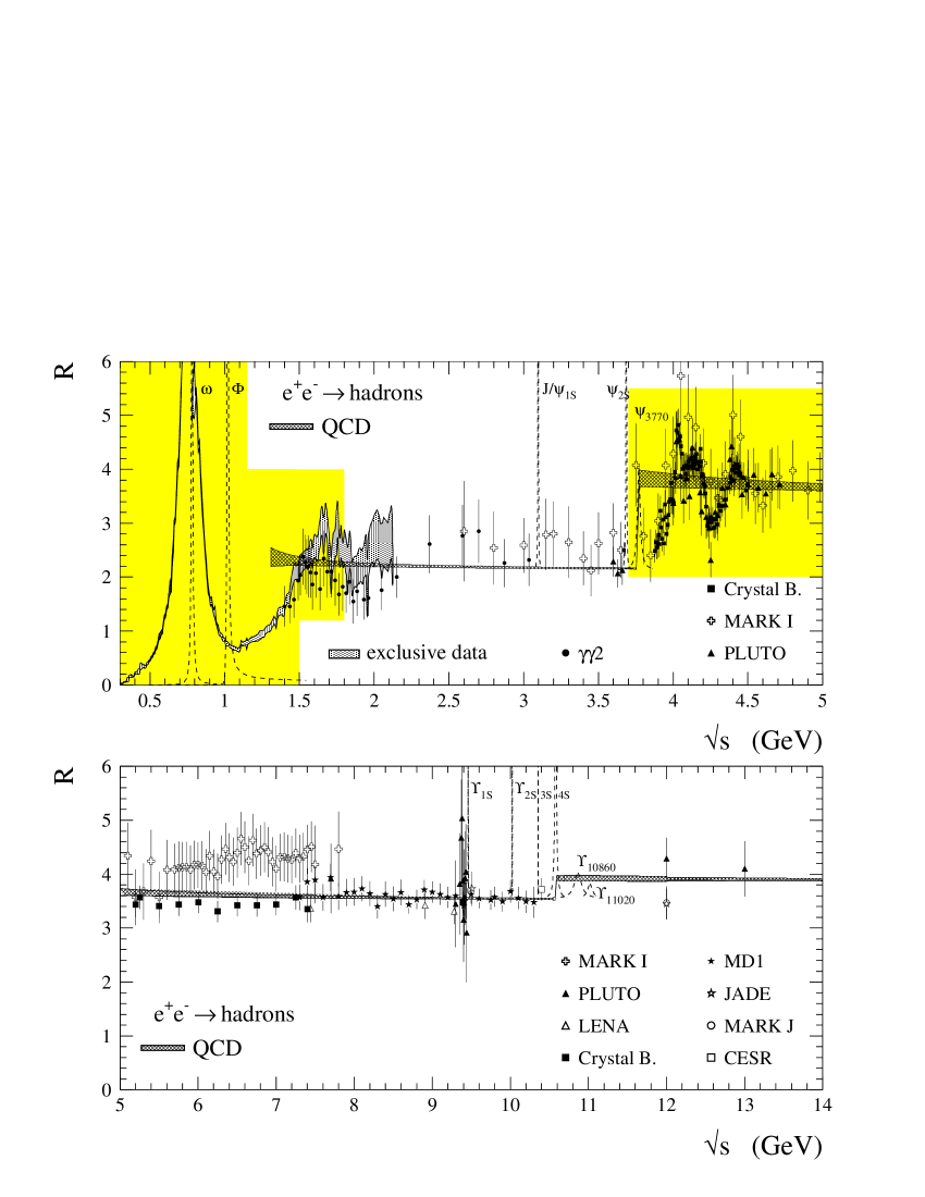
Figure 1: Inclusive hadronic cross section ratio in $e^{+}e^{-}$ annihilation versus the c.m. energy $\sqrt{s}$. Additionally shown is the QCD prediction of the continuum contribution as explained in the text. The shaded areas depict regions were experimental data are used for the evaluation of $\Delta\alpha_{\rm had}(M_{\rm Z}^{2})$ and $a_{\mu}^{\rm had}$ in addition to the measured narrow resonance parameters. The exclusive $e^{+}e^{-}$ cross section measurements at low c.m. energies are taken from DM1,DM2,M2N,M3N,OLYA,CMD,ND and $\tau$ data from ALEPH (see Ref. [1] for detailed information).

8 Results

According to Table 2, the combination of the theoretical and experimental evaluations of the integrals (5) and (7) yield the final results

$$\begin{array}[]{|rcl|}\hline\cr&&\\ ~{}~{}~{}\Delta\alpha_{\rm had}(M_{\rm Z}^{2})&=&(277.8\pm 2.2_{\rm exp}\pm 1.4_{\rm theo})\times 10^{-4}{}{}{}\\ &&\\ ~{}~{}~{}\alpha^{-1}(M_{\rm Z}^{2})&=&128.923\pm 0.030_{\rm exp}\pm 0.019_{\rm theo}{}{}{}\\ &&\\ ~{}~{}~{}a_{\mu}^{\rm had}&=&(695.1\pm 7.5_{\rm exp}\pm 0.7_{\rm theo})\times 10^{-10}{}{}{}\\ &&\\ ~{}~{}~{}a_{\mu}^{\rm SM}&=&(11\,659\,164.6\pm 7.5_{\rm exp}\pm 4.1_{\rm theo})\times 10^{-10}{}{}{}\\ &&\\ \hline\cr\end{array}$$ (25)

The total $a_{\mu}^{\rm SM}$ value includes an additional contribution from non-leading order hadronic vacuum polarization summarized in Refs. [38, 1] to be $a_{\mu}^{\rm had}[(\alpha/\pi)^{3}]\,=\,(-16.2\,\pm\,4.0)\times 10^{-10}$, where the error originates essentially from the uncertainty on the theoretical evaluation of the light-by-light scattering type of diagrams [39, 40].

Figure 2: Comparison of estimates of and $\Delta\alpha_{\rm had}(M_{\rm Z}^{2})$. The values are taken from Refs. [41, 32, 42, 43, 44, 1].

Fig. 2 shows a compilation of published results for the hadronic contribution $\Delta\alpha_{\rm had}(M_{\rm Z}^{2})$. Some authors give the hadronic contribution for the five light quarks only and add the top quark contribution of $\Delta\alpha_{\rm top}(M_{\rm Z}^{2})=-0.6\times 10^{-4}$ separately. This has been corrected for in the figure. The present inclusion of theoretical evaluations yields an improvement in the $\Delta\alpha_{\rm had}(M_{\rm Z}^{2})$ precision of a factor of two compared to our previous determination, $\alpha^{-1}(M_{\rm Z}^{2})=128.878\pm 0.085$ [1]. The improvement of the accuracy on $a_{\mu}^{\rm had}$ with respect to Ref. [1] where we found $a_{\mu}^{\rm had}$ $=(701.1\pm 9.3)\times 10^{-10}$ is also significant. Other estimates of $a_{\mu}^{\rm had}$ can be found in Refs. [32, 45, 46, 47].
The analysis using the spectral moments and also the measurement of $\alpha_{s}$ at the $\tau$ mass scale [9] showed concordantly that the OPE can be safely applied in order to predict integrals over inclusive spectra at relatively low energy scales. Nonperturbative contributions are indeed tiny and well below the envisaged precision. This approach leads to a large improvement in precision, as compared to the method used in Ref. [43] where perturbative QCD was assumed to be valid only above 3 GeV. Also the value used for $\alpha_{s}(M_{\rm Z}^{2})$ in the latter analysis was less precise than the current value. Finally, better and more complete experimental information, in particular at low energy, is used in the present work. Experimental data on $R$ are still necessary at very low energies and at the $c\bar{c}$ quark production threshold. Uncontrolled nonperturbative effects spoil the hadronic spectra and make the OPE approach unreliable. Thus, the final results on both, $\Delta\alpha_{\rm had}(M_{\rm Z}^{2})$ and $a_{\mu}^{\rm had}$, are still dominated by experimental uncertainties, where in particular the unmeasured $\pi^{+}\pi^{-}4\pi^{0}$ and ${\rm K}\bar{\rm K}\pi\pi$ low energy final states, which must be conservatively bound using isospin symmetry [1], as well as the two-pion final state in the latter case, contribute with large errors. Also more precise data of the $c\bar{c}$ continuum at threshold energies are needed.
We use the improved precision on $\alpha(M_{\rm Z}^{2})$ to repeat the global electroweak fit in order to adjust the mass of the Standard Model Higgs boson, $M_{\mathrm{Higgs}}$. As electroweak and heavy flavour input parameters we use values measured by the LEP, SLD, CDF, D0, CDHS, CHARM and CFFR collaborations, which have been collected and averaged in Ref. [2]. The prediction of the Standard Model is obtained from the ZFITTER electroweak library [48]. The fit adjusts $M_{\rm Z}$, $M_{\rm top}$ and $\alpha(M_{\rm Z})$ which are allowed to vary within their errors. Freely varying parameters are $\alpha_{s}$ and $M_{\rm Higgs}$. We obtain $\alpha_{s}(M_{\mathrm{Z}}^{2})\,=\,0.1198\,\pm\,0.0031$ in agreement with the experimental value of 0.122$\,\pm\,$0.006 [49] from the analyses of QCD observables in hadronic Z decays at LEP. The fitted Higgs boson mass is $129^{+103}_{-62}~{}{\rm GeV}$ with $\chi^{2}=16.4/15$, compared to $105^{+112}_{-62}~{}{\rm GeV}$ when using the previous value of $\alpha(M_{\rm Z}^{2})$ from Ref. [1]. An additional error of 50 GeV should be added to account for theoretical uncertainties [48]. Doing so, we obtain an upper limit for $M_{\mathrm{Higgs}}$ of 398 GeV at 95$\%$ CL.

Figure 3: Constraint fit results for the previous and the new value of $\alpha(M_{\rm Z}^{2})$ as a function of the Higgs mass.

Fig. 3 depicts the variation of $\Delta\chi^{2}$ as a function of the Higgs boson mass for the new and previously used values of $\alpha(M_{\rm Z}^{2})$ [1].

	$\Delta\,{\rm sin}^{2}\theta_{\rm eff}^{\rm lept}$
Experiment	0.00023
$\alpha(M_{\rm Z}^{2})$	0.00023 $\stackrel{{\scriptstyle\rm this~{}work}}{{\Longrightarrow}}$ 0.00010
$m_{t}$	0.00018
Theory	0.00014
$M_{\rm Higgs}$	0.00160 $[M_{\rm Higgs}=60$–$1000$ GeV$]$ $\stackrel{{\scriptstyle\rm F\/it}}{{\Longrightarrow}}$ $M_{\rm Higgs}=129^{+103}_{-62}~{}{\rm GeV}$

Table 3: Dominant uncertainties of input values of the Standard Model electroweak fit expressed in terms of $\Delta\,{\rm sin}^{2}\theta_{\rm eff}^{\rm lept}$ [2, 3].

Table 3 shows the dominant uncertainties of the input values of the Standard Model fit expressed in terms of $\Delta\,{\rm sin}^{2}\theta_{\rm eff}^{\rm lept}$. This work reduces the uncertainty of $\alpha(M_{\rm Z}^{2})$ on $M_{\rm Higgs}$ below the uncertainties from the experimental value of ${\rm sin}^{2}\theta_{\rm eff}^{\rm lept}$ or from the Standard Model, i.e., theoretical origin.

9 Conclusions

We have reevaluated the hadronic vacuum polarization contribution to the running of the QED fine structure constant, $\alpha(s)$, at $s=M_{\rm Z}^{2}$ and to the anomalous magnetic moment of the muon, $a_{\mu}$. We employed perturbative and nonperturbative QCD in the framework of the Operator Product Expansion in order to extend the energy regime where theoretical predictions are reliable. In addition to the theory, we used data from $e^{+}e^{-}$ annihilation and $\tau$ decays to cover low energies and quark thresholds. The extended theoretical approach reduces the uncertainty on $\Delta\alpha_{\rm had}(M_{\rm Z}^{2})$ by more than a factor of two. Our results are $\Delta\alpha_{\rm had}(M_{\rm Z}^{2})$ $=(277.8\pm 2.6)\times 10^{-4}$, propagating $\alpha^{-1}(0)$ to $\alpha^{-1}(M_{\rm Z}^{2})=(128.923\pm 0.036)$, and $a_{\mu}^{\rm had}=(695.1\pm 7.5)\times 10^{10}$ which yields the Standard Model prediction $a_{\mu}^{\rm SM}=(11\,659\,164.6\pm 8.5)\times 10^{-10}$. The new value for $\alpha(M_{\rm Z}^{2})$ improves the constraint on the mass of the Standard Model Higgs boson to $M_{\rm Higgs}=129^{+103}_{-62}~{}{\rm GeV}$.

References

- [1] R. Alemany, M. Davier and A. Höcker, Report LAL 97-02 (1997)
- [2] D. Ward, Talk given at ICHEP’97, Jerusalem 1997
- [3] A. Blondel, Talk given at ICHEP’96, Warsaw 1996
- [4] K.G. Wilson, Phys. Rev. 179 (1969) 1499
- [5] M.A. Shifman, A.L. Vainshtein and V.I. Zakharov, Nucl. Phys. B147 (1979) 385, 448, 519
- [6] F. Le Diberder and A. Pich, Phys. Lett. B289 (1992) 165
- [7] D. Buskulic et al. (ALEPH Collaboration), Phys. Lett. B307 (1993) 209
- [8] T. Coan et al. (CLEO Collaboration), Phys. Lett. B356 (1995) 580
- [9] A. Höcker, Talk given at the TAU’96 Conference, Colorado, 1996; R. Barate et al. (ALEPH Collaboration), to be published in Z. Phys.
- [10] N. Cabbibo and R. Gatto, Phys. Rev. Lett. 4 (1960) 313; Phys. Rev. 124 (1961) 1577.
- [11] A. Czarnecki, B. Krause and W.J. Marciano, Phys. Rev. Lett. 76 (1995) 3267; Phys. Rev. D52 (1995) 2619
- [12] S. Peris, M. Perrottet and E. de Rafael, Phys. Lett. B355 (1995) 523
- [13] R. Jackiw and S. Weinberg, Phys. Rev. D5 (1972) 2473
- [14] M. Gourdin and E. de Rafael, Nucl. Phys. B10 (1969) 667
- [15] S.J. Brodsky and E. de Rafael, Phys. Rev. 168 (1968) 1620
- [16] S. Adler, Phys. Rev. D10 (1974) 3714
-
[17]
L.R. Surguladze and M.A. Samuel,
Phys. Rev. Lett. 66 (1991) 560;
S.G. Gorishny, A.L. Kataev and S.A. Larin, Phys. Lett. B259 (1991) 144 - [18] S.A. Larin, T. van Ritbergen and J.A.M. Vermaseren, Phys. Lett. B400 (1997) 379
- [19] F. Le Diberder and A. Pich, Phys. Lett. B286 (1992) 147
- [20] D.J. Broadhurst, J. Fleischer and O.V. Tarasov, Z. Phys. C60 (1993) 287
- [21] K.G. Chetyrkin, J.H. Kühn and M. Steinhauser, Nucl. Phys. B482 (1996) 213
- [22] K.G. Chetyrkin, J.H. Kühn and A. Kwiatkowski, Phys. Rep. 277 (1996) 189
- [23] K.G. Chetyrkin and J.H. Kühn, Phys. Lett. B248 (1990) 359
- [24] S.A. Larin, T. van Ritbergen and J.A.M. Vermaseren, Phys. Lett. B405 (1997) 327
- [25] L.J. Reinders, H. Rubinstein and S. Yazaki, Phys. Rep. 127 (1985) 1
- [26] E. Braaten, S. Narison and A. Pich, Nucl. Phys. B373 (1992) 581
- [27] R.M. Barnett et al. (Particle Data Group), Phys. Rev. D54 (1996) 1
- [28] J. Flynn, Talk given at ICHEP’96, Warsaw 1996
- [29] R. Barate et al. (ALEPH Collaboration), Z. Phys. C76 (1997) 15
- [30] S. Chen, Talk given at QCD’97, Montpellier 1997
- [31] R.A. Bertlmann, Z. Phys. C39 (1988) 231
- [32] S. Eidelman and F. Jegerlehner, Z. Phys. C67 (1995) 585
- [33] M. Jamin and A. Pich, IFIC/97-06, FTUV/97-06, HD-THEP-96-55 (1997)
- [34] C. Bacci et al. ( Collaboration), Phys. Lett. B86 (1979) 234
- [35] J.L. Siegrist et al. (MARK I Collaboration), Phys. Rev. D26 (1982) 969
-
[36]
Z. Jakubowski et al. (Crystal Ball Collaboration),
Z. Phys. C40 (1988) 49;
C.Edwards et al. (Crystal Ball Collaboration), SLAC-PUB-5160 (1990) -
[37]
A.E. Blinov et al. (MD-1 Collaboration),
Z. Phys. C49 (1991) 239;
A.E. Blinov et al. (MD-1 Collaboration), Z. Phys. C70 (1996) 31 - [38] B. Krause, Phys. Lett. B390 (1997) 392
- [39] M. Hayakawa, T. Kinoshita and A.I. Sanda, Phys. Rev. D54 (1996) 3137; M. Hayakawa, T. Kinoshita and A.I. Sanda, Phys. Rev. Lett. 75 (1995) 790
- [40] J. Bijnens, E. Pallante and J. Prades, Nucl. Phys. B474 (1996) 379
- [41] B.W. Lynn, G. Penso and C. Verzegnassi, Phys. Rev. D35 (1987) 42
- [42] H. Burkhardt and B. Pietrzyk, Phys. Lett. B356 (1995) 398
- [43] A.D. Martin and D. Zeppenfeld, Phys. Lett. B345 (1995) 558
- [44] M.L. Swartz, Phys. Rev. D53 (1996) 5268
- [45] D.H. Brown and W.A. Worstell, Phys. Rev. D54 (1996) 3237
- [46] T. Kinoshita, B. Nižić and Y. Okamoto, Phys. Rev. D31 (1985) 2108
- [47] L.M. Barkov et al. (OLYA, CMD Collaboration), Nucl. Phys. B256 (1985) 365.
- [48] ‘Reports of the working group on precision calculations for the Z resonance’, Ed. D. Bardin et al., CERN-PPE 95-03
- [49] S. Bethke, Talk given at QCD’96, Montpellier 1996