An Analytic Extension of the $\overline{\mbox{MS}}$ Renormalization Scheme

Abstract

The conventional definition of the running coupling $\mbox{$\alpha_{\overline{\mbox{MS}}}$}(\mu)$ in quantum chromodynamics is based on a solution to the renormalization group equations which treats quarks as either completely massless at a renormalization scale $\mu$ above their thresholds or infinitely massive at a scale below them. The coupling is thus nonanalytic at these thresholds. In this paper we present an analytic extension of $\mbox{$\alpha_{\overline{\mbox{MS}}}$}(\mu)$ which incorporates the finite-mass quark threshold effects into the running of the coupling. This is achieved by using a commensurate scale relation to connect $\mbox{$\alpha_{\overline{\mbox{MS}}}$}(\mu)$ to the physical $\alpha_{V}$ scheme at specific scales, thus naturally including finite quark masses. The analytic-extension inherits the exact analyticity of the $\alpha_{V}$ scheme and matches the conventional $\overline{MS}$ scheme far above and below mass thresholds. Furthermore just as in $\alpha_{V}$ scheme, there is no renormalization scale ambiguity, since the position of the physical mass thresholds is unambiguous.

I Motivation

The running coupling in quantum chromodynamics (QCD) in the modified minimal subtraction ($\overline{\mbox{MS}}$) scheme [1] and other dimensional regularization schemes is traditionally constructed by solving the renormalization group equations using perturbative approximants to the $\beta$ function which change discontinuously at the quark mass thresholds [2, 3, 4]. This is equivalent to using effective Lagrangians with a fixed number of massless fermions in each energy range between the quark mass thresholds. Thus in the $\overline{\mbox{MS}}$ scheme, the $\beta(\mu)$ function depends on the number of “massless” quarks $N_{F}(\mu)$ which is taken as a step function of the renormalization scale $\mu$. Matching conditions at threshold require the equivalence of one effective theory with $n$ massless flavors to another effective theory with one massive and ($n-1$) massless quarks. It should be noted that this does not prevent one from including quark masses in the $\overline{\mbox{MS}}$ scheme. However, the quark masses do not enter into the $\beta$ function since the running of the coupling is mass independent.

The one-loop matching conditions [5, 6, 7] in the $\overline{\mbox{MS}}$ scheme require the coupling to be continuous if the matching is done at the quark masses, although the derivative is discontinuous. In two-loop matching [8, 9, 10] the coupling itself becomes discontinuous if the matching is done at the quark masses, but it can be rendered continuous by modifying the $\overline{\mbox{MS}}$ scheme [3]. Recently the three-loop matching conditions have been computed [10], which together with the four-loop $\beta$-function [11], give the possibility to evolve the $\overline{\mbox{MS}}$ coupling to four loops with massless quarks. This gives a reduced dependence on the matching scale, as shown in [12], but possibly a nonphysical threshold dependence. However, in such a treatment the derivatives of the coupling remain discontinuous. The inevitable result of the matching in a dimensional regularization scheme is that the running of the $\overline{\mbox{MS}}$ coupling in the renormalization scale is nonanalytic – nondifferentiable or even discontinuous – as the quark mass thresholds are crossed. Thus there is an intrinsic difficulty in expressing physical, smooth observables as an expansion in the $\overline{\mbox{MS}}$ coupling. It is clearly necessary to restore the finite quark mass effects in their entirety in order to restore analyticity.

Aesthetically, it is unnatural to characterize physical theories in terms of an artificially-constructed renormalization scheme such as $\overline{\mbox{MS}}$; it is more physical to use an effective charge as determined from experiment to define the fundamental coupling [13]. For example, in analogy to quantum electrodynamics, one could choose to define the QCD coupling as the coefficient $\alpha_{V}(Q)$ in the static limit of the scattering potential between two heavy quark-antiquark test charges:

$$V(Q^{2})=-4\pi C_{F}{\alpha_{V}(Q)\over Q^{2}}$$ (1)

at the momentum transfer $q^{2}=t=-Q^{2}$, where $C_{F}=({N_{C}^{2}-1})/({2N_{C}})={4}/{3}$ is the Casimir operator for the fundamental representation in $SU(N_{C})$, (with $N_{C}=3$ for QCD). Such an effective charge automatically incorporates the quark mass threshold effects in the running, and thus it has an analytic $\beta$ function. The $\alpha_{V}$ scheme is particularly well-suited to summing the effects of gluon exchange at low momentum transfer, such as in evaluating the final-state interaction corrections to heavy quark production [14], or in evaluating the hard-scattering matrix elements underlying exclusive processes [15]. A physical effective charge has the additional advantage that the Appelquist-Carazzone decoupling theorem [16] is automatically incorporated.

In this paper we shall construct an analytic extension of the $\alpha_{\overline{\mbox{MS}}}$ scheme, which we call ${\widetilde{\alpha}_{\overline{\mbox{MS}}}}$, by connecting the coupling directly to the analytic and physically-defined $\alpha_{V}$ scheme. The necessity for an analytic coupling has been emphasized by Shirkov and his collaborators[17]. Our definition allows one to use a scheme based on dimensional regularization, but which also, in a simple way, treats mass effects properly between the mass thresholds. Thus, instead of having the number of effective flavors ($N_{F}$) change discontinuously at (or nearby) the quark threshold, we obtain an analytic $N_{F}(\mu)$ which is a continuous function of the renormalization scale $\mu$ and the quark masses $m_{i}$. Thus the analytically-extended scheme inherits the mass dependence of the physical scheme. In addition, the renormalization scale $\mu$ that appears in the analytically-extended scheme ${\widetilde{\alpha}_{\overline{\mbox{MS}}}}$ is directly related to the momentum transfer appearing in the $\alpha_{V}$ scheme and thus has a definite and simple physical interpretation.

The essential advantage of the modified scheme ${\widetilde{\alpha}_{\overline{\mbox{MS}}}}$ is that it provides an analytic interpolation of conventional dimensional regularization expressions by utilizing the mass dependence of the physical $\alpha_{V}$ scheme. In effect, quark thresholds are treated analytically to all orders in $m^{2}/Q^{2}$; i.e., the evolution of our analytically extended coupling in the intermediate regions reflects the actual mass dependence of a physical effective charge and the analytic properties of particle production in a physical process. Just as in Abelian QED, the mass dependence of the effective potential and the analytically-extended scheme ${\widetilde{\alpha}_{\overline{\mbox{MS}}}}$ reflects the analyticity of the physical thresholds for particle production in the crossed channel. Furthermore, the definiteness of the dependence in the quark masses automatically constrains the renormalization scale. Alternatively, one could connect $\alpha_{\overline{\mbox{MS}}}$ to another physical charge such as $\alpha_{R}$ defined from $e^{+}e^{-}$ annihilation.

Our approach should be compared with the standard treatment of quark mass threshold effects in the $\overline{\mbox{MS}}$ scheme. For fixed order in $\alpha_{\mbox{{s}}}$ the corrections due to finite quark mass threshold effects which we are considering in this paper have been calculated for the hadronic width of the Z-boson and the $\tau$ lepton semihadronic decay rate [18, 19, 20, 9]. The calculations have been made both exactly to order ${\alpha}_{\overline{\mbox{MS}}}^{2}$ and as expansions in terms of $m^{2}/Q^{2}$ and $Q^{2}/m^{2}$ for light and heavy quarks respectively. Note that in principle the determination of the finite mass threshold effects for physical observables in dimensional regularization schemes would require a complete all-orders analysis of the higher-twist mass corrections to the effective Lagrangian of the theory.

There are a number of other reasons to construct an analytic extension of the $\alpha_{\overline{\mbox{MS}}}$ scheme:

• The comparison of the values of the coupling $\alpha_{\mbox{{s}}}$ as determined from different experiments and at different momentum scales is an essential test of QCD (for a recent review of existing measurements see [21]). One source of error is neglect of quark masses in the determination of $\alpha_{\mbox{{s}}}$ and in the subsequent running of the coupling from the scale where it has been determined to the conventional reference scale, the $Z$-boson mass.

• Lattice calculations for the J/$\Psi$ and $\Upsilon$ spectra now provide the most precise determination of $\alpha_{\mbox{{s}}}$ at low momentum scales[22, 23, 24, 25]. It is important to know how finite quark mass effects enter into the running of this value of $\alpha_{\mbox{{s}}}$ to lower and higher energy scales with as small an error as possible.

• Finite mass threshold effects in supersymmetric grand unified theories are important when analyzing the running and unification of couplings over very large ranges. It has been discussed, for example, in refs. [26, 27]. However, the scale used in the running and for the threshold effects has not been related to the physical scale which is naturally obtained in our approach.

• It is natural to unify theories by matching physical couplings and masses at the unification scale. This can be accomplished in the $\alpha_{V}$ scheme or equivalently ${\widetilde{\alpha}_{\overline{\mbox{MS}}}}$.

II Details of $\alpha_{V}$

In the case of the Abelian theory, the coupling $\alpha_{V}$ derived from the heavy lepton potential is equivalent to using the effective charge defined from the running of the photon propagator. In the non-Abelian theory the gluon propagator is not gauge invariant; one thus has to turn to a physical gauge invariant observable such as the heavy quark potential.

The effective charge ${\alpha_{V}(Q)}$, defined as in Eq. (1) can be calculated as a perturbation expansion in $\alpha_{\overline{\mbox{MS}}}$,

$$\alpha_{V}(Q) = \alpha_{\overline{\mbox{MS}}}(\mu)+v_{1,\overline{\mbox{MS}}}\left({Q\over\mu}\right){\alpha_{\overline{\mbox{MS}}}^{2}(\mu)\over\pi}+v_{2,\overline{\mbox{MS}}}\left({Q\over\mu}\right){\alpha_{\overline{\mbox{MS}}}^{3}(\mu)\over\pi^{2}}+\cdots$$ (2)

The first two nontrivial terms in the perturbative series have been computed in the $\overline{\mbox{MS}}$ scheme [28, 29, 30, 31, 32, 33]. A comprehensive analysis of $\alpha_{V}$ to order $\alpha^{3}$ has recently been given by M. Peter [33]:

$$v_{1,\overline{\mbox{MS}}}(\mu=Q) = -\frac{2}{3}N_{C}+\frac{5}{6}\beta_{0}\;=\;2.583-0.278N_{F}$$ (3)

$$v_{2,\overline{\mbox{MS}}}(\mu=Q) = \left(\frac{133}{144}+\frac{24\pi^{2}-\pi^{4}}{64}-\frac{11}{4}\zeta_{3}\right)N_{C}^{2}-\left(\frac{385}{192}-\frac{11}{4}\zeta_{3}\right)C_{F}N_{C}+$$ (5)

$$\frac{5}{6}\beta_{1}+\left[\left(\frac{35}{32}-\frac{3}{2}\zeta_{3}\right)C_{F}+\left(-\frac{217}{144}+\frac{7}{4}\zeta_{3}\right)N_{C}\right]\beta_{0}+\frac{25}{36}\beta_{0}^{2}$$

$$= 39.650-4.147N_{F}+0.0772N_{F}^{2}$$ (6)

where $\beta_{0}$ and $\beta_{1}$ are the first two universal coefficients in the $\beta$-function. It is also known that the next coefficient in the expansion is non-analytic in $\alpha=0$, since it contains a $\ln(\alpha)$ term [30]. This non-analyticity does not originate from fermionic corrections to the heavy quark potential. This can be seen by adopting a physical gauge. In such gauges we would reproduce the same analyticity structure for fermionic corrections in QCD as we find in QED. In QED, however, we have no problem with analyticity at any order in perturbation theory. Note that the total derivative of $\alpha_{V}$ with respect to the renormalization scale $\mu$ of the $\alpha_{\overline{\mbox{MS}}}$ scheme is zero, since $\alpha_{V}$ is a physical observable.

The scale ($Q$) dependence of the effective charge defines the equivalent of the Gell-Mann Low $\psi$-function for the effective charge in QED [34]. In the case of $\alpha_{V}$, $Q$ is the momentum transfer in the heavy quark potential, and the $\psi$-function is given by,

$$\frac{d\alpha_{V}(Q)}{d\ln Q}=-\psi^{(0)}\frac{\alpha_{V}^{2}}{\pi}-\psi^{(1)}\frac{\alpha_{V}^{3}}{\pi^{2}}-\psi_{V}^{(2)}\frac{\alpha_{V}^{4}}{\pi^{3}}-\psi_{V}^{(3)}\frac{\alpha_{V}^{5}}{\pi^{4}}-\cdots\;\;.$$ (7)

The first two terms in this series coincide with the universal and well-known first two terms in the Callan-Symanzik $\beta$-function [35], i.e. $\psi^{(0)}=\beta_{0}$ and $\psi^{(1)}=\beta_{1}$, but the higher order terms, $\psi_{V}^{(2)}$ etc., depends on the observable under study.

For completeness we give the coefficients in the QCD $\psi$ function with the normalization used above,

$$\psi^{(0)} = \frac{11}{6}N_{C}-\frac{1}{3}N_{F}=5.500-0.333N_{F}$$

$$\psi^{(1)} = \frac{17}{12}N_{C}^{2}-\frac{5}{12}N_{C}N_{F}-\frac{1}{4}C_{F}N_{F}=12.750-1.583N_{F}$$

$$\psi_{V}^{(2)} = \beta_{2,\overline{\mbox{MS}}}-\psi^{(1)}v_{1,\overline{\mbox{MS}}}-\psi^{(0)}v_{1,\overline{\mbox{MS}}}^{2}+\psi^{(0)}v_{2,\overline{\mbox{MS}}}$$

$$= \left(\frac{103}{48}+\frac{11(24\pi^{2}-\pi^{4})}{384}+\frac{121}{144}\zeta_{3}\right)N_{C}^{3}+$$

$$\left[\left(-\frac{445}{576}-\frac{24\pi^{2}-\pi^{4}}{192}-\frac{11}{9}\zeta_{3}\right)N_{C}^{2}+\right.$$

$$\left.\left(-\frac{343}{288}+\frac{11}{12}\zeta_{3}\right)N_{C}C_{F}+\frac{1}{32}C_{F}^{2}\right]N_{F}+$$

$$\left[\left(\frac{1}{576}+\frac{7}{36}\zeta_{3}\right)N_{C}+\left(\frac{23}{144}-\frac{1}{6}\zeta_{3}\right)C_{F}\right]N_{F}^{2}$$

$$= 193.074-27.014N_{F}+0.652N_{F}^{2}$$

The results given above in the $\alpha_{\overline{\mbox{MS}}}$ scheme have been obtained using massless QCD. The effects of non-vanishing quark masses can be taken into account by using a $Q^{2}$-dependent $N_{F}$ which will be derived from the one-loop massive vacuum polarization function in the next section.

III Calculation of the Running Coupling to One-Loop Order

Our approach in this paper is as follows: the $\mbox{$\alpha_{V}$}(Q)$ scheme automatically includes the effects of finite quark masses in the same manner that lepton masses appear in Abelian QED. We can then relate the $\overline{\mbox{MS}}$ scheme to the $\alpha_{V}$ scheme through a commensurate scale relation [36], which is effectively a scale transformation between the two schemes. The analytic dependence of $\alpha_{V}$ is then transferred to the analytically-extended ${\widetilde{\alpha}_{\overline{\mbox{MS}}}}$ scheme. The usual massless expressions are recovered far above or far below any individual quark mass threshold.

A Calculation of the Mass Dependence for the Running Coupling

The coupling $\mbox{$\alpha_{V}$}(Q)$, which is derived from heavy quark scattering, is closely related to the renormalization of the gluon propagator. In physical gauges with $Z_{1}=Z_{2}$ the coupling renormalization is due purely to self-energy insertions in the propagator.

For the purposes of this paper it will be sufficient to restrict our analysis to one-loop order, i.e. $\psi^{(0)}$.

The physical running coupling in the $\alpha_{V}$ scheme, normalized at an arbitrary momentum transfer scale $Q_{0}$, may be represented as

$$\mbox{$\alpha_{V}$}(Q)\equiv\frac{\alpha_{V}(Q_{0})}{1-\tilde{\Pi}\left(Q,Q_{0},\alpha_{V}(Q_{0})\right)}.$$ (8)

The vacuum polarization function $\tilde{\Pi}$ may be computed from the perturbative expansion of the renormalized propagator between heavy quarks. The coupling is then

$$\mbox{$\alpha_{V}$}(Q)=\alpha_{V}(Q_{0})\left[1+\tilde{\Pi}+\tilde{\Pi}^{2}+\tilde{\Pi}^{3}+\ .\ .\ .\right],$$ (9)

where we have used the shorthand $\tilde{\Pi}\equiv\tilde{\Pi}(Q,Q_{0},\alpha_{V}(Q_{0}))$ for the renormalized sum of all one-particle irreducible 1PI diagrams for the gluon self-energy. Since the coupling has the value $\alpha_{V}(Q_{0})\equiv\alpha_{0}$ at the physical renormalization point $Q=Q_{0}$, the self-energy obeys the boundary condition $\tilde{\Pi}(Q_{0},Q_{0},\alpha_{0})=0$.

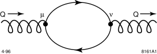
FIG. 1.: Single insertion of massive quark-antiquark loop into a gluon propagator, giving the quark part of the one-loop gluon vacuum polarization.

We begin by considering the integral representation of the quark part of the one-loop gluon vacuum polarization diagram (see Fig. 1):

$$\tilde{\Pi}^{(0)}_{\mbox{{q}}}(Q,Q_{0},\alpha_{0})=T_{F}\sum_{i=1}^{n}\frac{\alpha_{0}}{3\pi}\left(\int_{0}^{1}6z(1-z)\ln{\left(1+z(1-z)\rho_{i}(Q)\right)}-\right.$$

$$\left.\int_{0}^{1}6z(1-z)\ln{\left(1+z(1-z)\rho_{i}(Q_{0})\right)}\right)$$

where $\rho=Q^{2}/m^{2}$, $T_{F}={1\over 2}$, the superscript (0) indicates the one-loop order, the subscript q indicates the quark-part and the sum runs over all quarks ($n$). Thus the quark component of the one-loop $\psi$-function is:

$$\psi_{V,\mbox{{q}}}^{(0)}(Q)=-{\mbox{$N_{F,V}^{(0)}$}\over 3}=-\left[\frac{\pi}{\mbox{$\alpha_{V}$}^{2}}\frac{d\mbox{$\alpha_{V}$}}{d\ln{Q}}\right]^{(0)}_{\mbox{{q}}}=-\frac{\pi}{\alpha_{0}}\frac{d\,\tilde{\Pi}^{(0)}_{\mbox{{q}}}(Q,Q_{0},\alpha_{0})}{d\ln{Q}}.$$ (10)

This gives the contribution to $N_{F}$ from quark flavor $i$,

$$\mbox{$N_{F,V}^{(0)}$}(\rho_{i})=6\int_{0}^{1}\frac{z^{2}(1-z)^{2}\rho_{i}dz}{1+z(1-z)\rho_{i}}=1-\frac{6}{\rho_{i}}+\frac{24}{\rho_{i}^{3/2}\sqrt{4+\rho_{i}}}\tanh^{-1}{\sqrt{\frac{\rho_{i}}{\rho_{i}+4}}},$$ (11)

which is displayed in Fig. 2 as a function of $\rho$. Thus, by keeping the explicit quark mass dependence, $N_{F}$ becomes an analytic function of the scale $Q$.

FIG. 2.: The curve shows the contribution to the continuous $N_{F,V}^{(0)}$ for just one quark as a function of $\rho=Q^{2}/m^{2}$ where $m$ is the mass of the quark. $N_{F,V}^{(0)}$ is found by using the massive quark part of the one-loop gluon propagator instead of using the theta function thresholds conventionally used in dimensional regularization schemes.

In fact, the approximate form:

$$\mbox{$N_{F,V}^{(0)}$}(\rho_{i})\cong\left(1+{5\over\rho_{i}}\right)^{-1}$$ (12)

gives an accurate approximation to the exact form to within a percent over the entire range of the momentum transfer.

The one-loop analytic $N_{F,V}$ is shown in Fig. 3 for various quark flavors (for reference, the quark masses (in GeV) we used are: $m_{u}=.004$; $m_{d}=.008$; $m_{s}=.200$; $m_{c}=1.5$; $m_{b}=4.5$; $m_{t}=175$).

FIG. 3.: Continuous $N_{F,V}^{(0)}$ for various quarks, lightest to heaviest goes top to bottom (d, c, b, t as one proceed downwards; the u and s plots are virtually identical at this scale to the d). Q runs from 1 to $M_{Z}$ GeV (for reference, the quark masses (in GeV) used are: $m_{u}=.004$; $m_{d}=.008$; $m_{s}=.200$; $m_{c}=1.5$; $m_{b}=4.5$; $m_{t}=175$.)

We may now substitute the $N_{F,V}$ into the one-loop QCD $\psi$ function coefficient:

$$\psi_{V}^{(0)}(Q)=\frac{11}{2}-\frac{1}{3}\mbox{$N_{F,V}^{(0)}$}(\rho_{i})$$

and thence into the QCD one-loop renormalization group equation for the coupling constant:

$${{d\mbox{$\alpha_{V}$}}\over d\ln{Q}}=-\psi_{V}^{(0)}{\mbox{$\alpha_{V}$}^{2}\over\pi}$$ (13)

We may then solve this renormalization group equation to yield an expression for $\alpha_{V}$  which is analytic at mass thresholds. Note that the mass-dependence of the $\psi$ function applies specifically to the $\alpha_{V}$ scheme.

B Commensurate scale relation between $\alpha_{V}$ and $\alpha_{\overline{\mbox{MS}}}$ 

We now relate the mass dependence of the $\alpha_{V}$ scheme to the $\overline{\mbox{MS}}$ scheme using the commensurate scale relation [13, 36] between the two schemes. We use the NNLO results of Peter[33]. The first step is to invert Eq. (2) to obtain $\alpha_{\overline{\mbox{MS}}}$ as an expansion in $\alpha_{V}$,

$$\alpha_{\overline{\mbox{MS}}}(Q) = \alpha_{V}(M)+m_{1,V}\left({Q\over M}\right){\alpha_{V}^{2}(M)\over\pi}+m_{2,V}\left({Q\over M}\right){\alpha_{V}^{3}(M)\over\pi^{2}}+\cdots\;.$$ (14)

The needed commensurate scale relation is obtained by fixing the scales $M$ in Eq. (14) such that the $\psi^{(0)}$ and $\psi^{(1)}$ dependent parts of the coefficients $m_{1,V}$ and $m_{2,V}$ are absorbed into the running of the coupling $\alpha_{V}(M)$. This insures that all vacuum polarization dependence is summed into the heavy quark potential. Application of this procedure in next-to-next-to leading order (NNLO), using the multi-scale approach [36], gives the following scale-fixed relation between $\alpha_{V}$ and the conventional $\overline{\mbox{MS}}$,

$$\alpha_{\overline{\mbox{MS}}}(Q) = \alpha_{V}(Q^{*})+\frac{2}{3}N_{C}{\alpha_{V}^{2}(Q^{**})\over\pi}$$ (16)

$$+\left\{-\left(\frac{5}{144}+\frac{24\pi^{2}-\pi^{4}}{64}-\frac{11}{4}\zeta_{3}\right)N_{C}^{2}+\left(\frac{385}{192}-\frac{11}{4}\zeta_{3}\right)C_{F}N_{C}\right\}{\alpha_{V}^{3}(Q^{***})\over\pi^{2}}$$

$$= \alpha_{V}(Q^{*})+2{\alpha_{V}^{2}(Q^{**})\over\pi}+4.625{\alpha_{V}^{3}(Q^{***})\over\pi^{2}},$$ (17)

above or below the quark mass threshold. The coefficients in the perturbation expansion have their conformal values, i.e. the same coefficients would occur even if the theory had been conformally invariant with $\psi^{(0)}=0$ and thus do not contain the diverging $(\psi^{(0)}\alpha_{\mbox{{s}}})^{n}n!$ growth characteristic of an infrared renormalon [42]. The next-to leading order (NLO) coefficient $\frac{2}{3}N_{C}$ is a feature of the non-Abelian couplings of QCD and is not present in QED. The commensurate scales $Q^{*}$ and $Q^{**}$ are given by

$$Q^{*} = Q\exp\left[\frac{5}{6}\right]=2.300Q$$ (18)

$$Q^{**} = Q\exp\left[\left(\frac{105}{128}-\frac{9}{8}\zeta_{3}\right)\frac{C_{F}}{N_{C}}+\left(\frac{103}{192}+\frac{21}{16}\zeta_{3}\right)\right]=6.539Q$$ (19)

whereas to this order $Q^{***}$ is not constrained. However, a first approximation is obtained by setting $Q^{***}=Q^{**}$. Also note that $Q^{*}$ is unchanged when going from NLO to NNLO. The scale $Q^{*}$ arises because of the convention used in defining the modified minimal subtraction scheme. Comparing the scales $Q$ and $Q^{*}$ we find that the scale in the $\overline{\mbox{MS}}$ scheme ($Q$) is a factor $\sim 0.4$ smaller than the physical scale ($Q^{*}$).

Alternatively, one can write the relation between $\alpha_{\overline{\mbox{MS}}}$ and $\alpha_{V}$ as a single-scale commensurate scale relation [42]. In this procedure $Q^{*}=Q^{**}$ where

$$Q^{*} = Q\exp\left[\frac{5}{6}+\left[\left(\frac{35}{32}-\frac{3}{2}\zeta_{3}\right)C_{F}-\left(\frac{19}{48}-\frac{7}{4}\zeta_{3}\right)N_{C}\right]\frac{\alpha_{V}}{\pi}\right]$$ (20)

The conformal coefficients are the same in the two procedures. However, the single-scale form has the advantage that the non-Abelian perturbation theory matches in a simple way the corresponding Abelian perturbation theory in the limit $N_{C}\to 0$ with $C_{F}\alpha_{s}$ and $N_{F}/C_{F}$ fixed [43]. For $N_{C}=3$ we have $\ln(Q^{*}/Q)=5/6+4.178\alpha_{V}/\pi.$

C Definition of the Analytic ${\widetilde{\alpha}_{\overline{\mbox{MS}}}}$ 

We now adopt the commensurate scale relation with the effective charge of the effective potential as a definition of the extended scheme ${\widetilde{\alpha}_{\overline{\mbox{MS}}}}$:

$$\widetilde{\alpha}_{\overline{\mbox{MS}}}(Q)=\alpha_{V}(Q^{*})+\frac{2N_{C}}{3}{\alpha_{V}^{2}(Q^{**})\over\pi}+\cdots,$$ (21)

for all scales $Q$. Eq. (21) not only provides an analytic extension of dimensionally regulated schemes, but it also ties down the renormalization scale to the physical masses of the quarks as they enter into the vacuum polarization contributions to $\alpha_{V}$. There is thus no scale ambiguity in perturbative expansions in $\alpha_{V}$ or ${\widetilde{\alpha}_{\overline{\mbox{MS}}}}$.

Taking the logarithmic derivative of the commensurate scale relation given by Eq. (21) with respect to $\ln Q$ we can define the $\psi$-function for the ${\widetilde{\alpha}_{\overline{\mbox{MS}}}}$ scheme as follows,

$$\widetilde{\psi}_{\overline{\mbox{MS}}}(Q)\equiv\psi_{V}(Q^{*})+2\frac{2N_{C}}{3}{\alpha_{V}(Q^{**})\over\pi}\psi_{V}(Q^{**}).$$ (22)

To lowest order this gives $\widetilde{\psi}_{\overline{\mbox{MS}}}^{(0)}(Q)=\psi_{V}^{(0)}(Q^{*})$, which in turn gives the following relation between $\widetilde{N}_{F,\overline{\mbox{MS}}}^{(0)}$ and $N_{F,V}^{(0)}$,

$$\widetilde{N}_{F,\overline{\mbox{MS}}}^{(0)}(Q)=N_{F,V}^{(0)}(Q^{*}),$$ (23)

where to lowest order, $Q^{*}=\exp(5/6)Q$.

We can also use the approximate form given by Eq. (12) to write

$$\widetilde{N}_{F,\overline{\mbox{MS}}}^{(0)}(\rho_{i})\cong\left(1+{5\over\rho_{i}{\exp({5\over 3})}}\right)^{-1}\cong\left(1+{1\over{\rho_{i}}}\right)^{-1}.$$ (24)

In other words the contribution from one flavor is $\simeq 0.5$ when the scale $Q$ equals the quark mass $m_{i}$. Thus the standard procedure of matching $\alpha_{\overline{\mbox{MS}}}(\mu)$ at the quark masses is a zeroth order approximation to the continuous $N_{F}$.

FIG. 4.: The continuous $\widetilde{N}_{F,\overline{\mbox{MS}}}^{(0)}$ in the analytic extension of the $\overline{\mbox{MS}}$ scheme as a function of the physical scale $Q$. (For reference the continuous $N_{F}$ is also compared with the conventional procedure of taking $N_{F}$ to be a step-function at the quark-mass thresholds.)

Adding all flavors together gives the total $\widetilde{N}_{F,\overline{\mbox{MS}}}^{(0)}(Q)$ which is shown in Fig. 4. For reference the continuous $N_{F}$ is also compared with the conventional procedure of taking $N_{F}$ to be a step-function at the quark-mass thresholds. The figure shows clearly that there are hardly any plateaus at all for the continuous $\widetilde{N}_{F,\overline{\mbox{MS}}}^{(0)}(Q)$ in between the quark masses. Thus there is really no scale below 1 TeV where $\widetilde{N}_{F,\overline{\mbox{MS}}}^{(0)}(Q)$ can be approximated by a constant. In other words, for all $Q$ below 1 TeV there is always one quark with mass $m_{i}$ such that $m_{i}^{2}\ll Q^{2}$ or $Q^{2}\gg m_{i}^{2}$ is not true. We also note that if one would use any other scale than the BLM-scale for $\widetilde{N}_{F,\overline{\mbox{MS}}}^{(0)}(Q)$, the result would be to increase the difference between the analytic $N_{F}$ and the standard procedure of using the step-function at the quark-mass thresholds.

D Comparing the Analytic $\mbox{${\widetilde{\alpha}_{\overline{\mbox{MS}}}}$}(Q)$ with $\alpha_{\overline{\mbox{MS}}}$ 

We can obtain the renormalization group equation for the analytic extension of the $\overline{\mbox{MS}}$ coupling $\widetilde{\alpha}_{\overline{\mbox{MS}}}$ by using $\widetilde{N}_{F,\overline{\mbox{MS}}}^{(0)}(Q)$, etc.:

$${d\,\widetilde{\alpha}_{\overline{\mbox{MS}}}(Q)\over d\ln Q}=-\widetilde{\psi}_{\overline{\mbox{MS}}}^{(0)}(Q){\widetilde{\alpha}_{\overline{\mbox{MS}}}^{2}(Q)\over\pi}+\cdots.$$ (25)

The solution to Eq. (25) provides an analytic scale-fixed extension of $\mbox{$\alpha_{\overline{\mbox{MS}}}$}(\mu)$, which we have denoted as ${\widetilde{\alpha}_{\overline{\mbox{MS}}}}$. The result can be compared with the standard method of computing $\alpha_{\overline{\mbox{MS}}}$, based on the evolution with distinct $\psi$ functions for different quark mass regimes. When doing this comparison one has to keep in mind that it is possible to take quark mass threshold effects into account also in the $\overline{\mbox{MS}}$ scheme when calculating an observable. In the next section we will compare our analytic extension of the $\overline{\mbox{MS}}$ scheme with the standard treatment of quark mass threshold effects for the hadronic width of the Z-boson. However, for most observables the quark mass threshold effects are not known and thus it is also important to compare ${\widetilde{\alpha}_{\overline{\mbox{MS}}}}$ and $\alpha_{\overline{\mbox{MS}}}$ directly.

FIG. 5.: The solid curve shows the relative difference between the solutions to the 1-loop renormalization group equation using continuous $N_{F}$, $\widetilde{\alpha}_{\overline{\mbox{MS}}}(Q)$, and conventional discrete theta-function thresholds, $\alpha_{\overline{\mbox{MS}}}(Q)$. The dashed (dotted) curves shows the same quantity but using the scale $2Q$ ($Q/2$) in $\widetilde{N}_{F,\overline{\mbox{MS}}}^{(0)}$. The solutions have been obtained numerically starting from the world average [21] $\alpha_{\overline{\mbox{MS}}}(M_{Z})=0.118$.

Fig. 5 shows the relative difference between the two different solutions of the 1-loop renormalization group equation, i.e. $(\widetilde{\alpha}_{\overline{\mbox{MS}}}(Q)-{\alpha}_{\overline{\mbox{MS}}}(Q))/\widetilde{\alpha}_{\overline{\mbox{MS}}}(Q)$. The solutions have been obtained numerically starting from the world average [21] $\alpha_{\overline{\mbox{MS}}}(M_{Z})=0.118$. The figure shows that taking the quark masses into account in the running leads to effects of the order of one percent, most especially pronounced near thresholds.

In addition the figure shows the results obtained by using two different scales in $\widetilde{N}_{F,\overline{\mbox{MS}}}^{(0)}(Q)$, namely $2Q$ and $Q/2$, when solving Eq. (25). This shows clearly that the BLM-scale minimizes the difference between solutions using the continuous and discontinuous $N_{F}$. The other two scale choices gives differences of several percent for small $Q$.

We see from the figure that the effect of treating thresholds continuously can be of the order of a few percent in the magnitude of the QCD coupling when running down from $M_{Z}$ to $m_{c}$. This is a significant difference, at the level of the precision of current $\alpha_{\mbox{{s}}}$ determinations. The primary factor which influences the running is the value of the one-loop $\psi$ function, $\psi^{(0)}=\frac{11}{2}-\frac{1}{3}N_{F}$: a larger value of $N_{F}$ gives a smaller $\psi^{(0)}$ and makes $\alpha_{\mbox{{s}}}$ run more slowly; conversely a smaller value of $N_{F}$ gives a larger $\psi^{(0)}$ and $\alpha_{\mbox{{s}}}$ runs more quickly.

We can trace the difference in the couplings as follows: at $M_{Z}$, the continuous function $\widetilde{N}_{F,\overline{\mbox{MS}}}^{(0)}$ is above the discrete threshold value of 5, but goes below it at 30 GeV; it remains below the discrete threshold value until $m_{b}$ where it becomes larger and remains larger until $\sim$ 3 GeV, where it becomes smaller again etc.

Thus, running down from $M_{Z}$, ${\widetilde{\alpha}_{\overline{\mbox{MS}}}}$ runs slower than $\alpha_{\overline{\mbox{MS}}}$ until 30 GeV where the difference between them begins to close as ${\widetilde{\alpha}_{\overline{\mbox{MS}}}}$ runs faster than $\alpha_{\overline{\mbox{MS}}}$; at $\sim$ 8 GeV the difference starts to increase again until the $b$ quark threshold where ${\widetilde{\alpha}_{\overline{\mbox{MS}}}}$ starts to run slower than $\alpha_{\overline{\mbox{MS}}}$ and the difference between the two decreases until $\sim$ 3 GeV, etc. this behavior forms the peaks seen in Fig. 5. Thus we see that ${\widetilde{\alpha}_{\overline{\mbox{MS}}}}$ will end up higher than $\alpha_{\overline{\mbox{MS}}}$ when running down to low momentum transfers starting from $M_{Z}$.

IV Applications

In this section we will show how to compute an observable using the analytic extension of the $\overline{\mbox{MS}}$ scheme and compare with the standard treatment of quark mass threshold effects in the $\overline{\mbox{MS}}$ scheme. The essential difference between the perturbative expansions in the $\alpha_{\overline{\mbox{MS}}}$ and ${\widetilde{\alpha}_{\overline{\mbox{MS}}}}$ couplings are terms that contain quark masses. In the analytic scheme the quark mass effects are automatically included whereas in the $\overline{\mbox{MS}}$ scheme they have to be included by hand for each observable.

For some observables, such as the hadronic width of the Z-boson and the $\tau$ lepton semihadronic decay rate, corrections due to non-zero quark masses have been calculated within the $\overline{\mbox{MS}}$ scheme [18, 19, 20, 9]. To be specific we are interested in the so called double bubble diagrams where the outer quark loop which couples to the weak current is considered massless and the inner quark loop is massive. Other types of mass corrections, such as the double triangle graphs where the external current is electroweak, are not taken into account by the analytic extension of the $\overline{\mbox{MS}}$ scheme. (For a recent review of higher order corrections to the Z-boson width see [44].)

To illustrate how to compute an observable using the analytic extension of the $\overline{\mbox{MS}}$ scheme and compare with the standard treatment in the $\overline{\mbox{MS}}$ scheme we consider the QCD corrections to the quark part of the non-singlet hadronic width of the Z-boson, $\Gamma_{had,q}^{NS}$. Writing the QCD corrections in terms of an effective charge we have

$$\Gamma_{had,q}^{NS}=\frac{G_{F}M_{Z}^{3}}{2\pi\sqrt{2}}\sum_{q}\{(g_{V}^{q})^{2}+(g_{A}^{q})^{2}\}\left[1+\frac{3}{4}C_{F}\frac{\alpha_{\Gamma,q}^{NS}(s)}{\pi}\right]$$ (26)

where the effective charge $\alpha_{\Gamma,q}^{NS}(s)$ contains all QCD corrections,

$$\frac{\alpha_{\Gamma,q}^{NS}(s)}{\pi} = \frac{\alpha_{\overline{\mbox{MS}}}^{(N_{L})}(\mu)}{\pi}\left\{1+\frac{\alpha_{\overline{\mbox{MS}}}^{(N_{L})}(\mu)}{\pi}\left[\sum_{q=1}^{N_{L}}\left(-\frac{11}{12}+\frac{2}{3}\zeta_{3}+F\left(\frac{m_{q}^{2}}{s}\right)-\frac{1}{3}\ln\left(\frac{\mu}{\sqrt{s}}\right)\right)\right.\right.$$ (28)

$$\left.\left.+\sum_{Q=N_{L}+1}^{6}G\left(\frac{m_{Q}^{2}}{s}\right)\right]+\ldots\right\}$$

The functions $F$ and $G$ are the effects of non-zero quark masses for light and heavy quarks, respectively. In the following we will not restrict ourselves to the case $\sqrt{s}=M_{Z}$ since we want to compare the two treatments of masses for arbitrary $s$. Thereby the number of light flavors $N_{L}$ will also vary with $s$. We will also assume that the matching of $N_{F}$ is done at the quark masses. Thus a quark with mass $m<\mu$ is considered as light whereas a quark with mass $m>\mu$ is considered as heavy.

To calculate $\alpha_{\Gamma,q}^{NS}(s)$ in the analytic extension of the $\overline{\mbox{MS}}$ scheme one first has to apply the BLM scale-setting procedure which absorbs all the massless effects of non-zero $N_{F}$ into the running of the coupling. This gives,

$$\frac{\alpha_{\Gamma,q}^{NS}(s)}{\pi} = \frac{\alpha_{\overline{\mbox{MS}}}^{(N_{L})}(Q^{*})}{\pi}\left\{1+\frac{\alpha_{\overline{\mbox{MS}}}^{(N_{L})}(Q^{*})}{\pi}\left[\sum_{q=1}^{N_{L}}F\left(\frac{m_{q}^{2}}{s}\right)+\sum_{Q=N_{L}+1}^{6}G\left(\frac{m_{Q}^{2}}{s}\right)\right]+\ldots\right\}$$ (29)

where

$$Q^{*}=\exp\left[3\left(-\frac{11}{12}+\frac{2}{3}\zeta_{3}\right)\right]\sqrt{s}=0.7076\sqrt{s}.$$ (30)

Operationally, one next simply drops all the mass dependent terms in the above expression and replaces the fixed $N_{F}$ coupling $\alpha_{\overline{\mbox{MS}}}^{(N_{L})}$ with the analytic ${\widetilde{\alpha}_{\overline{\mbox{MS}}}}$. (For an observable calculated with massless quarks this step reduces to replacing the coupling.) In this way both the massless $N_{F}$ contribution as well as the mass dependent contributions from double bubble diagrams are absorbed into the coupling and we are left with a very simple expression,

$$\frac{\alpha_{\Gamma,q}^{NS}(s)}{\pi} = \frac{\mbox{${\widetilde{\alpha}_{\overline{\mbox{MS}}}}$}(Q^{*})}{\pi}.$$ (31)

This simple expression reflects the fact that the effects of quarks in the perturbative coefficients, both massless and massive, should be absorbed into the running of the coupling.

To compare with the ordinary $\overline{\mbox{MS}}$ treatment we need the functions $F$ and $G$ in Eq. (29). Expansions in terms of $m^{2}/s$ and $s/m^{2}$ can be found in [18, 19, 9] whereas they have been calculated numerically in [20]. In addition the $\alpha_{\mbox{{s}}}^{3}$ correction due to heavy quarks has been calculated as an expansion in $s/m^{2}$ in [9]. It should also be noted that the function $G$ was first calculated for QED [45]. Here we will use the following expansions,

$$F\left(\frac{m^{2}}{s}\right) = \left(\frac{m^{2}}{s}\right)^{2}\left[\frac{13}{3}-4\zeta_{3}-\ln\left(\frac{m^{2}}{s}\right)\right]$$ (33)

$$+\left(\frac{m^{2}}{s}\right)^{3}\left[\frac{136}{243}+\frac{16}{27}\zeta_{2}+\frac{56}{81}\ln\left(\frac{m^{2}}{s}\right)-\frac{8}{27}\ln^{2}\left(\frac{m^{2}}{s}\right)\right]$$

$$G\left(\frac{m^{2}}{s}\right) = \frac{s}{m^{2}}\left[\frac{44}{675}+\frac{2}{135}\ln\left(\frac{s}{m^{2}}\right)\right]+\left(\frac{s}{m^{2}}\right)^{2}\left[-\frac{1303}{1058400}-\frac{1}{2520}\ln\left(\frac{s}{m^{2}}\right)\right]$$ (34)

which are good to within a few percent for $m^{2}/s<0.25$ and $s/m^{2}<4$ respectively. We will also use the relation [20],

$$F\left(\frac{m^{2}}{s}\right)=G\left(\frac{m^{2}}{s}\right)+\frac{1}{6}\ln\left(\frac{m^{2}}{s}\right)-\left(-\frac{11}{12}+\frac{2}{3}\zeta_{3}\right)$$ (35)

to get $F$ in the interval $0.25<m^{2}/s<1$ since the expansion of $F$ in terms of $m^{2}/s$ breaks down for $m^{2}/s>0.25$.

Before carrying out the comparison of the analytic extension of the $\overline{\mbox{MS}}$ scheme with the standard treatment it is instructive to look at the effective contribution to $\alpha_{\Gamma,q}^{NS}(s)$ from one flavor with mass $m$ as a function of $s$. To make the arguments more transparent we will use the renormalization scale $\mu=\sqrt{s}$ when doing this. For small $s$, when the quark is considered heavy the contribution is given by $G(m^{2}/s)$ whereas for larger $s$ the quark is considered as light and contributes with $F(m^{2}/s)-\frac{11}{12}+\frac{2}{3}\zeta_{3}$. Normalizing to the massless contribution $-\frac{11}{12}+\frac{2}{3}\zeta_{3}$ gives the contribution to the effective $N_{F}$ in the $\alpha_{\mbox{{s}}}^{2}$-coefficient,

$$N_{F,\overline{\mbox{MS}}}^{\mbox{{eff}}}\left(\frac{s}{m^{2}}\right)=\left\{\begin{array}[]{lc}{\displaystyle\frac{G\left({\frac{m^{2}}{s}}\right)}{-{\frac{11}{12}+\frac{2}{3}\zeta_{3}}}}&\quad\text{for $\sqrt{s}<m$ }\\ \\ {\displaystyle\frac{F\left({\frac{m^{2}}{s}}\right)-{\frac{11}{12}+\frac{2}{3}\zeta_{3}}}{-{\frac{11}{12}+\frac{2}{3}\zeta_{3}}}}&\quad\text{for $\sqrt{s}>m$ }\end{array}\right.\quad,$$ (36)

which is shown in Fig. 6 as a function of $s/m^{2}$.

FIG. 6.: The effective contribution to $N_{F}$ in the $\alpha_{\mbox{{s}}}^{2}$-coefficient in the standard $\overline{\mbox{MS}}$ scheme from a quark with mass $m$ as a function of $s/m^{2}$ (using $\mu=\sqrt{s}$). The discontinuity between the two expansions in $s/m^{2}$ and $m^{2}/s$ can be seen at the nonanalytic point $s/m^{2}=4$.

At first it might seem unnatural that the effective contribution to $N_{F}$ in the $\alpha_{\mbox{{s}}}^{2}$-coefficient is negative for heavy quarks. However, this is a characteristic feature of the standard $\overline{\mbox{MS}}$ scheme which arises from the fact that the number of flavors in the running of the coupling is kept constant. Starting from a scale well below the threshold the number of flavors in the running as well as in the $\alpha_{\mbox{{s}}}^{2}$ coefficient is not affected by the heavy quark. As the threshold is approached from below the number of flavors in the running should increase which would make the running of the coupling slower (since $\psi^{(0)}$ would be smaller) which in turn should lead to a larger $\alpha_{\overline{\mbox{MS}}}$. But, since the number of flavors is kept constant in the running this effect has to be taken into account by adding a positive contribution to the $\alpha_{\mbox{{s}}}^{2}$-coefficient, i.e. the function $G$. Since the massless contribution is negative this means that the contribution to $N_{F}$ becomes negative for a heavy quark. Once the threshold has been crossed the number of flavors in the running changes and the need to compensate for a too small $\alpha_{\overline{\mbox{MS}}}$ vanishes rapidly as the scale is increased above the threshold. For scales well above the threshold the mass-effects are negligible and the massless result is regained as $F$ goes to zero. This should be compared with the analytic $\overline{\mbox{MS}}$ scheme where $N_{F}$ is increased continuously in the running.

To compare the analytic extension of the $\overline{\mbox{MS}}$ scheme with the standard $\overline{\mbox{MS}}$ result for $\alpha_{\Gamma,q}^{NS}(s)$ we will apply the BLM scale-setting procedure also for the standard $\overline{\mbox{MS}}$ scheme. This is to ensure that any differences are due to the different ways of treating quark masses and not due to the scale choice. In other words we want to compare Eqs. (29) and (31). As the normalization point we use $\alpha_{\overline{\mbox{MS}}}^{(5)}(M_{Z})=0.118$ which we evolve down to $Q^{*}=0.7076M_{Z}$ using leading order massless evolution with $N_{F}=5$. This value is then used to calculate $\alpha_{\Gamma,q}^{NS}(M_{Z})=0.1243$ in the $\overline{\mbox{MS}}$ scheme using Eq. (29). Finally, Eq. (31) gives the normalization point for $\mbox{${\widetilde{\alpha}_{\overline{\mbox{MS}}}}$}(Q^{*})$.

FIG. 7.: The relative difference between the calculation of $\alpha_{\Gamma,q}^{NS}(s)$ in the analytic extension of the $\overline{\mbox{MS}}$ scheme and the standard treatment of masses in the $\overline{\mbox{MS}}$ scheme. The discontinuities are due to the mismatch between the $s/m^{2}$ and $m^{2}/s$ expansions of the functions $F$ and $G$.

Fig. 7 shows the relative difference between the two expressions for $\alpha_{\Gamma,q}^{NS}(s)$ given by Eqs. (29) and (31) respectively. As can be seen from the figure the relative difference is smaller than 0.2% for scales above 1 GeV. Thus the analytic extension of the $\overline{\mbox{MS}}$ scheme takes the mass corrections into account in a very simple way without having to include an infinite series of higher dimension operators or doing complicated multi-loop diagrams with explicit masses.

V Conclusion

An essential feature of the $\alpha_{V}$(Q) scheme is that there is no renormalization scale ambiguity, since $Q^{2}$ is the physical momentum transfer. The $\alpha_{V}$ scheme naturally takes into account quark mass thresholds, which is of particular phenomenological importance to QCD applications in the intervening mass region between those thresholds. In this paper we have utilized commensurate scale relations to provide an analytic extension of the conventional $\overline{\mbox{MS}}$  scheme in which many of the advantages of the $\alpha_{V}$ scheme are inherited by the ${\widetilde{\alpha}_{\overline{\mbox{MS}}}}$ scheme, but only minimal changes have to be made to the standard $\alpha_{\overline{\mbox{MS}}}$ scheme. Given the commensurate scale relation, Eq. (16), connecting ${\widetilde{\alpha}_{\overline{\mbox{MS}}}}$ to $\alpha_{V}$  expansions in ${\widetilde{\alpha}_{\overline{\mbox{MS}}}}$ are effectively expansions in $\alpha_{V}$ to the given order in perturbation theory at a corresponding commensurate scale. Unlike the conventional $\alpha_{\overline{\mbox{MS}}}$ scheme, the modified ${\widetilde{\alpha}_{\overline{\mbox{MS}}}}$ scheme is analytic at quark mass thresholds, and it thus provides a natural expansion parameter for perturbative representations of observables. In the Abelian limit $N_{C}\to 0$, ${\widetilde{\alpha}_{\overline{\mbox{MS}}}}$ scheme agrees with the standard effective charge method of QED.

We have found that taking finite quark mass effects into account analytically in the running, rather than using a fixed $N_{F}$ between thresholds, leads to effects of the order of one percent for the one-loop running coupling, with the largest differences occurring near thresholds. These differences are important for observables that are calculated neglecting quark masses and could in principle turn out to be significant in comparing low and high energy measurements of the strong coupling.

We have also found that our extension of the $\overline{\mbox{MS}}$ scheme, including quark mass effects analytically, reproduces the standard treatment of quark masses in the $\overline{\mbox{MS}}$ scheme to within a fraction of a percent. The standard treatment amounts to either calculating multi-loop diagrams with explicit quark masses or adding higher dimension operators to the effective Lagrangian. These corrections can be viewed as compensating for the fact that the number of flavors in the running is kept constant between mass thresholds. By utilizing the BLM scale setting procedure, based on the massless $N_{F}$ contribution, the analytic extension of the $\overline{\mbox{MS}}$ scheme correctly absorbs both massless and mass dependent quark contributions from QCD diagrams, such as the double bubble diagram, into the running of the coupling. This gives the opportunity to convert a calculation made in the $\overline{\mbox{MS}}$ scheme with massless quarks into an expression which includes quark mass corrections from QCD diagrams by using the BLM scale and replacing $\alpha_{\overline{\mbox{MS}}}$ with ${\widetilde{\alpha}_{\overline{\mbox{MS}}}}$.

For simplicity we have analyzed the mass corrections arising from analyticity only to leading order in QCD. For further precision, our analysis will need to be systematically improved. For example, at higher orders the commensurate scale relation connecting $\alpha_{V}$ to $\alpha_{\overline{\mbox{MS}}}$ will have to be corrected with finite mass effects. We have seen that the BLM scale minimizes the difference between the analytic and the conventional $\alpha_{\overline{\mbox{MS}}}$-coupling. Thus, these kinds of corrections are not likely to decrease the difference between the analytic and the conventional $\alpha_{\overline{\mbox{MS}}}$-coupling.

Finally, we note the potential importance of utilizing the $\alpha_{V}$ effective charge or the equivalent analytic ${\widetilde{\alpha}_{\overline{\mbox{MS}}}}$ scheme in supersymmetric and grand unified theories, particularly since the unification of couplings and masses would be expected to occur in terms of physical quantities rather than parameters defined by theoretical convention.

REFERENCES

- [1] W.A. Bardeen et al., Phys. Rev. D 18, 3998 (1978).
- [2] R.M. Barnett, H.E. Haber, D.E. Soper, Nucl. Phys. B 306, 697 (1988).
- [3] W.J. Marciano, Phys. Rev. D 29, 580 (1984).
- [4] G. Rodrigo, A. Santamaria, Phys. Lett. B313, 441 (1993).
- [5] S. Weinberg, Phys. Lett. 91B, 51 (1980).
- [6] L. Hall, Nucl. Phys. B178, 75 (1981).
- [7] P. Binetruy, T. Schucker, Nucl. Phys B178, 293, 307 (1981).
- [8] W. Wetzel, Nucl. Phys. B196, 259 (1982); W. Bernreuther and W. Wetzel, Nucl. Phys. B197, 228 (1982); W. Bernreuther, Ann. Phys. 151, 127 (1983); Z. Phys. C 20, 331 (1983).
- [9] S.A. Larin, T. van Ritbergen, J.A.M. Vermaseren, Nucl. Phys. B438, 278 (1995).
- [10] K.G. Chetyrkin, B.A. Kniehl, M. Steinhauser, Phys. Rev. Lett. 79, 2184 (1997).
- [11] T. van Ritbergen, J.A.M. Vermaseren, S.A. Larin, Phys. Lett. B400, 379 (1997).
- [12] G. Rodrigo, A. Pich, A. Santamaria, hep-ph/9707474.
- [13] S.J. Brodsky, G.P. Lepage and P.B. Mackenzie, Phys. Rev. D28, 228 (1983).
- [14] S.J. Brodsky, A.H. Hoang, J.H. Kuhn, T. Teubner, Phys. Lett. B359, 355 (1995).
- [15] S.J. Brodsky, C-R. Ji, A. Pang, D.G. Robertson, hep-ph/9705221.
- [16] T. Appelquist and J. Carazzone, Phys. Rev. D11, 2856 (1975).
- [17] D.V. Shirkov, TMP, 3, 466, (1992). See also K.A. Milton, O. P. Solovtsova, hep-ph/9710316, and references therein.
- [18] K.G. Chetyrkin, Phys. Lett. B 307, 169 (1993).
- [19] A.H. Hoang, M. Jeżabek, J.H. Kühn, T. Teubner, Phys. Lett. B 338, 330 (1994).
- [20] D.E. Soper and L.R. Surguladze, Phys. Rev. Lett. 73, 2958 (1994).
- [21] P.N. Burrows, Acta Phys. Polon. B28, 701 (1997).
- [22] J. Shigemitsu, hep-lat/9608058, review talk at Lattice 96, Unpublished.
- [23] C.T.H. Davies et al., hep-lat/9510006, Lattice 1995:409-416, Unpublished.
- [24] C.T.H. Davies et al., Phys. Lett. B 345, 42 (1995).
- [25] C.T.H. Davies et al., Phys. Rev. D56, 2755 (1997)
- [26] L. Clavelli, P.W. Coulter, UAHEP-954, Jul 1995, hep-ph/9507261.
- [27] J.A. Bagger, K.T. Matchev, D.M. Pierce, Phys. Lett. B348, 443 (1995). D.M. Pierce, J.A. Bagger, K.T. Matchev, R. Zhang, Nucl. Phys. B491, 3 (1997)
- [28] L. Susskind, Coarse grained quantum chromodynamics, lectures given at Les Houches 1976, in R. Balin and C. H. Llewellyn Smith (eds.), Weak and Electromagnetic Interactions At High Energies, (North-Holland 1977, 207-308).
- [29] W. Fischler, Nucl. Phys. B129, 157 (1977).
- [30] T. Appelquist, M. Dine, I.J. Muzinich, Phys. Lett. 69B, 231 (1977); Phys. Rev. D17, 2074 (1978).
- [31] F.L. Feinberg, Phys. Rev. Lett 39, 316 (1977); Phys. Rev. D17, 2659 (1978); S. Davis, F.L. Feinberg, Phys. Lett. 78B, 90 (1978).
- [32] A. Billoire, Phys. Lett. 92B, 343 (1980).
- [33] M. Peter, Phys. Rev. Lett. 78, 602 (1997); Nucl. Phys. B 501, 471 (1997).
- [34] M. Gell-Mann and F.E. Low, Phys. Rev. 95, 1300 (1954).
- [35] C.G. Callan, Phys. Rev. D2, 1541 (1970); K. Symanzik, Commun. Math. Phys. 18, 227 (1970).
- [36] S.J. Brodsky, H.J. Lu, Phys. Rev. D51, 3652 (1995); hep-ph/9506322.
- [37] R. Giles and L. McLerran, Phys. Lett. 79B, 447 (1978).
- [38] M. Melles, hep-ph/9805216; S.J. Brodsky, M.S. Gill, M. Melles, J. Rathsman in preparation.
- [39] H. Georgi and H.D. Politzer, Phys. Rev. D14, 1829 (1976).
- [40] D.A. Ross, Nucl. Phys. B140, 1 (1978).
- [41] O. Puzyrko, in progress.
- [42] S.J. Brodsky, G.T. Gabadadze, A.L. Kataev, H.J. Lu, Phys. Lett. B372, 133 (1996).
- [43] S.J. Brodsky and P. Huet, hep-ph/9707543.
- [44] B.A. Kniehl, Int. Journ. of Mod. Phys. A 10, 443 (1995).
- [45] B.A. Kniehl, Phys. Lett. B237, 127 (1990).