[

Larger Domains from Resonant Decay of Disoriented Chiral Condensates

Abstract

The decay of disoriented chiral condensates into soft pions is considered within the context of a linear sigma model. Unlike earlier analytic studies, which focused on the production of pions as the sigma field rolled down toward its new equilibrium value, here we focus on the amplification of long-wavelength pion modes due to parametric resonance as the sigma field oscillates around the minimum of its potential. This process can create larger domains of pion fluctuations than the usual spinodal decomposition process, and hence may provide a viable experimental signature for chiral symmetry breaking in relativistic heavy ion collisions; it may also better explain physically the large growth of domains found in several numerical simulations.

]

Experiments at the Relativistic Heavy Ion Collider at Brookhaven and at the Large Hadron Collider at CERN may soon be able to probe many questions in strong-interaction physics which have until now been studied only on paper or simulated on a lattice. One major area of study concerns the QCD chiral phase transition. In relativistic heavy ion collisions, it is possible that non-equilibrium dynamics could produce “disoriented chiral condensates” (DCCs), domains in which a particular direction of the pion field develops a non-zero expectation value.[1, 2, 3] These domains would then decay to the usual QCD vacuum by radiating soft pions. Preliminary searches for DCCs by the MiniMax Collaboration in $p\overline{p}$ collisions at Fermilab have thus far not found evidence for the production and decay of DCCs [4], though they are far more likely to be created in upcoming heavy ion collisions. Thus, understanding their possible formation and likely decay signatures in anticipation of further experimental work is of key importance.
If these domains grow to sufficient size (on the order of 3 - 7 fm), such an experimental event would be marked by a particular clustering pattern: some regions within the detector would measure a large number of charged pions but few neutral pions, while other regions of the detector would measure predominantly neutral pions with few charged pions.[2] Defining ${\cal R}$ to be the ratio of neutral pions to total pions, ${\cal R}\equiv n_{\pi^{o}}/(n_{\pi^{o}}+n_{\pi^{+}}+n_{\pi^{-}})$, it has been demonstrated that the probability for measuring various ratios ${\cal R}$ in DCC events obeys $P({\cal R})=(4{\cal R})^{-1/2}$, which, especially for small-${\cal R}$, may be easily distinguished from the isospin-invariant result of $P({\cal R})\rightarrow\delta({\cal R}-1/3)$. [2] (Detecting the decay of such DCCs could be improved by measuring the two-pion correlation functions [5], and from enhanced dilepton and photoproduction [6], in addition to studying the fraction of neutral pions produced.) The production and subsequent relaxation of such DCCs may also explain the so-called “Centauro” high-energy cosmic ray events, in which very large numbers of charged pions are detected with only very few neutral pions. [2, 7]
However, as emphasized in [8, 9], if the disoriented domains do not grow to such large scales within heavy ion collisions, such experimental signatures become less and less easy to distinguish from the isospin-invariant case. Even if DCCs are produced following a heavy ion collision, if the domains do not grow to be “large” (that is, several fm), then the detector would sample so many of these discrete domains within a given run, each of which with the pion field aligned along some random direction, that the clustering effects would be washed out. A crucial question, then, is whether or not sufficiently large domains might grow in the nonequilibrium aftermath of a heavy ion collision.
Several authors have considered the amplification of long-wavelength pion modes from the decay of DCCs in the context of a linear sigma model.[2, 6, 8, 9] The relevant degrees of freedom are modeled by the scalar fields $\sigma$ and $\vec{\pi}$, which may be grouped together as $\Phi=(\sigma,\vec{\pi})$. Above the critical temperature, when the system is in the chirally-symmetric state, the effective potential for $\Phi$ is $O(4)$ symmetric, and $\langle\Phi\rangle=0$. To model a strongly-nonequilibrium situation, Rajagopal and Wilczek considered a quench: as the quark-gluon plasma in the interaction region between the colliding nuclei expands and cools, the effective temperature may fall quickly to $T\ll T_{c}$. Because the zero-temperature potential is not chirally-symmetric, domains form, and it takes some time for the fields to evolve from $\langle\sigma\rangle=\langle\vec{\pi}\rangle=0$ to the new equilibrium values, $\langle\sigma\rangle\neq 0$, $\langle\vec{\pi}\rangle=0$. Following the quench, the fields relax to these new equilibrium values according to the effective potential, $V(\Phi)={\lambda\over 4}(\Phi^{2}-v^{2})^{2}-H\sigma$; that is, the $\sigma$ field ‘rolls down’ from $\sigma\sim 0$ to $\sigma\sim v$.
Numerical simulations [2, 3] reveal a large amplification of soft pion modes from the relaxation of the nonequilibrium plasma. Previous authors have attempted to explain these numerical results analytically in terms of spinodal decomposition: during the time that $\sigma$ rolls down toward $v$, pion modes with wavelengths satisfying $k^{2}\leq\lambda(v^{2}-\langle\Phi^{2}\rangle)$ will grow exponentially. However, under the usual quench scenario, the time it takes for $\sigma$ to roll to $v$, and hence the maximum domain size for the DCCs, remains too small to produce clear experimental signatures. Under this scenario, domains typically remain pion-sized, $\sim 1.4$ fm. (See, e.g., [8, 9].) This physical mechanism alone therefore remains incapable of explaining the large domains found in numerical simulations.
Building on earlier work in [10], we consider here a physically distinct process which could produce larger domains of DCC, and hence might better explain the significant clustering observed in numerical simulations. Rather than amplification of pion modes while $\sigma$ rolls down its potential hill, we focus on the parametric amplification of pion modes as $\sigma$ oscillates around the minimum of its potential. Because this is a distinct process, the growth of domains due to parametric resonance, unlike the growth of domains due to spinodal decomposition, may reach scales on the order of 3-5 fm.
This means of DCC decay is similar to cosmological post-inflation reheating. An early attempt was made to apply the reheating formalism of [11] to the decay of DCCs due to parametric resonance in [10]. However, the analytic tools for studying the nonequilibrium, nonperturbative dynamics of such resonant decays have improved since this early work on reheating, and the earlier approximations, while at times qualitatively informative, prove quantitatively unreliable. Most important, this earlier study [10] approximated $\sigma$’s oscillations as purely periodic, in which case the equation of motion for the pionic fluctuations reduces to the well-known Mathieu equation. Ignoring the nonlinear, anharmonic terms (such as $\lambda\sigma^{4}$) in the evolution of $\sigma$ then yields the prediction of an infinite hierarchy of resonance bands, with decreasing characteristic exponents. Yet given the nonlinear equation for $\sigma$, the equation of motion for the pions reduces instead to a Lamé equation, which, in the cases of interest, has only one single resonance band, with a different value for the amplified modes’ characteristic exponent. As emphasized in [12], these two differences combined can change dramatically the predicted spectra from parametric resonance; to be useful in making contact with experiments, these nonlinearities must be attended to, as in the present study. (Furthermore, the authors of [10] did not consider the size of domains created by the parametric resonance, as considered here.) Instead, we draw on the more recent studies of reheating in [12, 13, 14, 15] to consider the question of DCCs and their resonant decay.
Following [2], we consider a quench scenario: the temperature of the plasma drops quickly from above the critical temperature (with $\langle\Phi\rangle=0$) to near zero. The effective Lagrangian density following the quench is given by

$${\cal L}=-\textstyle{{1\over 2}}(\partial_{\mu}\Phi)^{2}-\textstyle{{\lambda\over 4}}\left(\Phi^{2}-v^{2}\right)^{2}+H\sigma.$$ (1)

Here $H$ is an external field which breaks the chiral symmetry and picks out the $\sigma$ direction as the true minimum. The pion mass is proportional to $H$. The true vacuum is characterized by $\langle\Phi\rangle=(f_{\pi},\vec{0})$, where $f_{\pi}=92.5$ MeV is the pion decay constant. In the limit as $H\rightarrow 0$, $f_{\pi}\rightarrow v$. In the following, we neglect $H$ in the resulting equations of motion, but add by hand a pion mass $m_{\pi}=135$ MeV; we also set $\lambda=20.0$ and $v=87.4$ MeV, which yield $m_{\sigma}=(2\lambda f_{\pi}^{2}+m_{\pi}^{2})^{1/2}=600$ MeV. These standard values for the parameters are chosen, as in [2, 8, 9, 10], to fit low-energy pion dynamics.
As a first approximation, we neglect effects due to the expansion of the plasma. Obviously the expansion of the plasma plays a crucial role, at least for early times following the collision, in dropping the temperature below the critical temperature. (Some work has been done to incorporate analytically the effects of cosmological expansion in the resonant decay of a massive inflaton [14], which may be useful in improving future analytic studies of DCCs and their decay). We also ignore noise and other medium-related effects on the resonance; as demonstrated in the context of post-inflation reheating, such effects do not generally destroy the parametric resonance, but rather enhance it. [16]
We study the nonequilibrium, nonperturbative dynamics by means of a Hartree approximation, by writing $\sigma(t,{\bf x})=\sigma_{0}(t)+\delta\sigma(t,{\bf x})$, and replacing $\vec{\pi}^{3}\rightarrow 3\langle\vec{\pi}^{2}\rangle\>\vec{\pi}$ and $\vec{\pi}^{2}\rightarrow\langle\vec{\pi}^{2}\rangle$. The vacuum expectation value may be written in terms of the field’s associated (Fourier-transformed) mode functions as $\langle\vec{\pi}^{2}\rangle=\int d^{3}k\>|\vec{\pi}_{k}|^{2}/(2\pi)^{3}$. Because the $\delta\sigma$ fluctuations decouple from the pion modes in this approximation, we will focus below on the pionic fluctuations.
Within a given DCC domain, the pion field will be aligned along some particular direction, $\hat{n}_{\pi}$, in isospin space. We will therefore write $\vec{\pi}=\chi\>\hat{n}_{\pi}$. In terms of the dimensionless variables $\tau\equiv\sqrt{\lambda v^{2}}\>t$ and $\kappa\equiv k/\sqrt{\lambda v^{2}}$, and the scaled field $\varphi(\tau)\equiv\sigma_{0}(t)/v$, the coupled equations of motion take the form:

$$\varphi^{\prime\prime}+\left(\varphi^{2}-1+\Sigma_{\pi}\right)\varphi \simeq 0,$$ (2)

$$\chi_{k}^{\prime\prime}+\left(p^{2}+\varphi^{2}+\Sigma_{\pi}\right)\chi_{k} \simeq 0,$$ (3)

where primes denote $d/d\tau$, and we have defined

$$M\equiv m_{\pi}/\sqrt{\lambda v^{2}},\>\>p^{2}\equiv\kappa^{2}+M^{2}-1,\>\>\Sigma_{\pi}\equiv\langle\vec{\pi}^{2}\rangle/v^{2}.$$ (4)

Note that with the values of the parameters assumed here, $\sqrt{\lambda v^{2}}=390.9$ MeV, and $M^{2}=0.12$. These equations of motion are conformally equivalent to those for massless fields in an expanding, spatially-open universe, and hence we may apply the techniques of [15] to study their solutions.
We are interested in the growth of $\vec{\pi}$ modes as $\sigma_{0}$ oscillates around $v$. Having begun, following the quench, near $\sigma_{0}\sim 0$, $\sigma_{0}$ will roll down its potential hill toward $v$. The rolling field will at first overshoot the minimum at $v$, and then begin oscillating around $v$. The amplitude of these oscillations will eventually be damped by the transfer of energy from this oscillating zero mode into the $\vec{\pi}$ fluctuations. For early times after these oscillations have begun, however, the amplitude of $\sigma_{0}$ will remain nearly constant. In this strongly-coupled system, unlike in the weakly-coupled inflationary case, the $\sigma$ field will execute only a few oscillations before settling in to its minimum. Yet, as we see below, even these few oscillations could prove significant, since most particle production via parametric resonance occurs in highly non-adiabatic bursts, when the velocity of the oscillating field passes through zero. [11] Furthermore, because the system has been quenched from its initial, chirally-symmetric state, we assume that $\Sigma_{\pi}$ is small at the beginning of $\sigma_{0}$’s oscillations. (The fact that spinodal decomposition alone cannot produce large DCC domains is equivalent to $\Sigma_{\pi}$ remaining small while $\sigma$ rolls down its potential hill.) Then we may solve the coupled equations for early times after the oscillations have begun, and study the growth of the fluctuations $\vec{\pi}_{k}$. Because $\sigma_{0}$ begins oscillating quasi-periodically, certain pion modes will be amplified due to parametric resonance.
The resonance will fade once the backreaction term, $\Sigma_{\pi}$, grows to be of the same order as the tree-level terms, such as $\varphi^{2}$. To study the behavior of the pionic fluctuations, we solve the coupled equations of (3) for early times after the beginning of $\sigma_{0}$’s oscillations, when $\Sigma_{\pi}$ may be neglected. This lasts up to the time $\tau_{\rm end}$, determined by $\Sigma_{\pi}(\tau_{\rm end})=\overline{\varphi^{2}(\tau)}$, where an overline denotes time-averaging over a period of $\varphi$’s oscillations.
Assuming that $\sigma_{0}$’s oscillations begin once $\sigma_{0}$ reaches its inflection point, $\sigma_{\rm infl}=v/\sqrt{3}$, it will roll past the minimum and up to the point at which $V(\sigma)=V(\sigma_{\rm infl})$, before rolling back down through $v$. This sets $\varphi_{0}=\sqrt{5/3}$. Because this definition of the initial amplitude is somewhat arbitrary, we study the resonance effects for $\varphi_{0}$ in the range $1\leq\varphi_{0}\leq\sqrt{2}$. In the range $1\leq\varphi_{0}\leq\sqrt{2}$, $\varphi(\tau)$ oscillates as [12]

$$\varphi(\tau)=\varphi_{0}\>{\rm dn}\left(\gamma\tau,\>\nu\right),$$ (5)

where ${\rm dn}(u,\nu)$ is the third Jacobian elliptic function, $\gamma\equiv\varphi_{0}/\sqrt{2}$, and $\nu\equiv\sqrt{2(1-\varphi_{0}^{-2})}$. Eq. (5) holds for $\tau\leq\tau_{\rm end}$. The ${\rm dn}$-function oscillates between a maximum at 1 and a minimum at $(1-\nu^{2})^{1/2}$, with a period of $2K(\nu)/\gamma$, where $K(\nu)$ is the complete elliptic integral of the first kind. [17]
With $\varphi(\tau)$ oscillating as in Eq. (5), the equation of motion for $\chi_{k}$ becomes the Lamé equation of order one. A solution for the pion modes $\chi_{k}(\tau)$ may thus be written in the form [12, 13, 15, 18]:

$$U_{k}^{(\pm)}(\tau)=A(\tau)\exp\left(\pm\mu_{\kappa}(\nu)\gamma\tau\right).$$ (6)

Here $A(\tau)$ is a periodic function, normalized to have unit amplitude, and $\mu_{\kappa}(\nu)$ is the characteristic exponent (also known as the Floquet index). The form of $\mu_{\kappa}$ depends on both $\kappa$ and $\nu$. Clearly, whenever $Re\left[\mu_{\kappa}(\nu)\right]\neq 0$, the coupled modes will be exponentially amplified. The exact relation between the $U_{k}$ modes and $\chi_{k}$ (and hence $\vec{\pi}$) depends on the assumed initial conditions following the nonequilibrium quench. If we make the usual assumption, that $\chi_{k}(\tau_{0})=1/\sqrt{2\omega_{p}(\tau_{0})}$ and $\chi_{k}^{\prime}(\tau_{0})=-i\sqrt{\omega_{p}(\tau_{0})/2}$, with $\omega_{p}^{2}(\tau)\equiv p^{2}+\varphi^{2}(\tau)$ [12, 19], then the $\chi_{k}$ modes may be written as a linear combination of $U_{k}^{(\pm)}$ as in [12, 13, 15].
In [15], these coupled equations were studied for the range $\varphi_{0}\geq\sqrt{2}$. Proceeding in exactly the same way, solutions may be found for the case $1\leq\varphi_{0}\leq\sqrt{2}$. The characteristic exponent has non-zero real parts only within a single resonance band, given by

$$\left(\textstyle{{1\over 2}}-M^{2}\right)-\textstyle{{1\over 2}}\sqrt{1-\varphi_{0}^{2}\left(2-\varphi_{0}^{2}\right)}\leq\kappa^{2}$$ (7)

$$\leq\left(\textstyle{{1\over 2}}-M^{2}\right)+\textstyle{{1\over 2}}\sqrt{1-\varphi_{0}^{2}\left(2-\varphi_{0}^{2}\right)}.$$ (8)

The resonance band includes modes with $k\leq m_{\pi}$ for all values of $\varphi_{0}\geq 1.23$, that is, even for amplitudes of the oscillating field smaller than $\varphi_{0}=\sqrt{5/3}$. As in [15], $\mu_{\kappa}(\nu)$ may be written in terms of a complete elliptic integral of the third kind. The real part of $\mu_{\kappa}(\nu)$ is plotted in Fig. 1. Near the center of the resonance band for a given value of $\varphi_{0}$, $Re\left[\mu_{\kappa}\right]\sim 0.1-0.3$. Note that as in the numerical simulations of [2, 3], the strongest amplification (indicating greatest particle production) occurs for $k\leq m_{\pi}$. The maximum values of $Re\left[\mu_{\kappa}\right]$ fall in the $k\rightarrow 0$ limit.

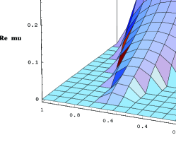
FIG. 1.: $Re\left[\mu_{\kappa}(\nu)\right]$ as a function of both the dimensionless momentum, $\kappa$, and the dimensionless initial amplitude of $\sigma_{0}$’s oscillations, $\varphi_{0}$. In these units, $m_{\pi}=0.35$; the largest exponents, and hence the strongest resonance, occur for $k\leq m_{\pi}$.

Given $Re\left[\mu_{\kappa}\right]$, one can determine $\tau_{\rm end}$, based on the growth of $\Sigma_{\pi}$. If $\tau_{\rm end}$ is large enough, then observable domains of DCC could be formed and detected. Within a given domain, $\Sigma_{\pi}(\tau)$ is given as an integral over $|\chi_{k}(\tau)|^{2}$. To evaluate $\tau_{\rm end}$, we solve numerically the equation

$$\Sigma_{\pi}(\tau_{\rm end})=\int_{\rm res.\>band}\frac{d\kappa\>\kappa^{2}}{2\pi^{2}}|\chi_{k}(\tau_{\rm end})|^{2}=\overline{\varphi^{2}},$$ (9)

where the integral extends over the single resonance band. The time-average of the (dimensionless) oscillating $\sigma$ field, $\overline{\varphi^{2}}$, may be written in terms of $E(\nu)$, the complete elliptic integral of the second kind, using the integral of ${\rm dn}^{2}(u,\nu)$ over a period of its oscillations (see [17]). Eq. (9) then yields $t_{\rm end}\sim 5$ fm/$c$ over most of the range $1\leq\varphi_{0}\leq\sqrt{2}$. This should be compared with the usual spinodal decomposition scenario, in which the pionic fluctuations would be exponentially amplified only for the brief period $t_{\rm spinodal}\simeq\sqrt{2}/m_{\sigma}\simeq 0.47$ fm/$c$.
In order to find the characteristic sizes to which DCC domains may grow before the parametric resonance is damped, we may follow [20] and evaluate the two-point correlation function:

$$D(t,\>{\bf r}) \equiv \langle\vec{\pi}(t,\>{\bf r})\vec{\pi}(t,\>{\bf 0})\rangle=\int\frac{d^{3}k}{(2\pi)^{3}}e^{i{\bf k}\cdot{\bf r}}|\vec{\pi}_{k}|^{2}$$ (10)

$$= (\lambda v^{2})^{-3/2}\int\frac{d\kappa\>\kappa^{2}}{2\pi^{2}}j_{0}(\kappa x)|\chi_{k}(\tau)|^{2},$$ (11)

with the dimensionless length defined by ${\bf x}\equiv\sqrt{\lambda v^{2}}\>{\bf r}$. We have also used $\vec{\pi}_{k}(t)=\chi_{k}(\tau)\>\hat{n}_{\pi}$ within a given domain. We may solve this integral in the saddle-point approximation, making use of Eq. (11.4.29) of [17], with the result that

$$D(t,\>{\bf r}) \propto \Sigma_{\pi}(t)\exp\left(-r^{2}/\xi_{D}^{2}(t)\right),$$ (12)

$$\xi_{D}^{2}(t) \equiv 4\gamma|Re\left(\partial^{2}\mu_{\kappa}(\nu)/\partial\kappa^{2}\right)|_{\kappa_{\rm max}}(t/\sqrt{\lambda v^{2}}).$$ (13)

Eq. (13) reveals that the domain size grows as $t^{1/2}$. The maximum correlation length, $\xi_{D}(t_{\rm end})$, is plotted in Fig. 2.

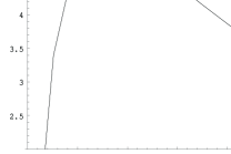
FIG. 2.: Maximum domain size for DCCs, $\xi_{D}(t_{\rm end})$, as a function of $\varphi_{0}$, in units of fm.

Over much of the range $1\leq\varphi_{0}\leq\sqrt{2}$, $\xi_{D}(t_{\rm end})$ lies between 3 - 5 fm. The usual spinodal decomposition process, in the absence of the ‘annealing’ studied in [9], on the other hand, can only create domains of order 1.4 fm. [8]. If ‘annealing’ is effective, domains from spinodal decomposition may grow to $3-4$ fm; yet independent of the dynamics as $\sigma$ rolls down its potential hill, it still must end its evolution by oscillating around $v$, and the resonant production of pions would follow as studied here.
Parametric resonance offers a promising means of producing observable signals from the production and decay of disoriented chiral condensates in the aftermath of relativistic heavy ion collisions. Unlike spinodal decomposition alone, this physical process may explain the signficant growth of DCCs found in numerical simulations. Future analytic studies should better include effects from the expansion of the plasma, and from $\delta\sigma-\vec{\pi}$ and $\vec{\pi}-\vec{\pi}$ scatterings, which are neglected here in the Hartree approximation. If these effects remain subdominant, however, then the resonant decay of DCCs should produce low-momentum pions with a distribution observably distinct from the isospin-invariant case.
It is a pleasure to thank Krishna Rajagopal, Dan Boyanovsky, Stanislaw Mrowczynski, and Hisakazu Minakata for helpful discussions. This research was supported in part by NSF grant PHY-98-02709.

REFERENCES

- [1] A. A. Anselm, Phys. Lett. B217, 169 (1989); A. A. Anselm and M. G. Ryskin, Phys. Lett. B266, 482 (1991); J. D. Bjorken, Acta Phys. Pol. B23, 561 (1991); J. P. Blaizot and A. Krzywicki, Phys. Rev. D 46, 246 (1992), and 50, 442 (1994).
- [2] K. Rajagopal and F. Wilczek, Nucl. Phys. 399, 395 (1993) and B404, 577 (1993).
- [3] Z. Huang and X. N. Wang, Phys. Rev. D 49, 442 (1994); M. Asakawa, Z. Huang, and X. N. Wang, Phys. Rev. Lett. 74, 3126 (1995); F. Cooper et al., Phys. Rev. D 50, 2848 (1994), D 51, 2377 (1994), C 54, 3298 (1996); D. Boyanovsky et al., Phys. Rev. D 51, 734 (1995) and 54, 1748 (1996); M. A. Lampert et al., Phys. Rev. D 54, 2213 (1996); J. Randrup, Phys. Rev. D 55, 1188 (1997), Phys. Rev. Lett. 77, 1226 (1996).
- [4] T. Brooks et al., Phys. Rev. D 55, 5667 (1997).
- [5] H. Hiro-Oka and H. Minakata, Phys. Lett. B425, 129 (1998).
- [6] D. Boyanovsky et al., Phys. Rev. D 56, 3929 (1997) and 56, 5233 (1997); Y. Kluger et al., Phys. Rev. C 57, 280 (1998).
- [7] L. T. Baradzei et al., Nucl. Phys. B370, 365 (1992).
- [8] S. Gavin, A. Gocksch, and R. D. Pisarski, Phys. Rev. Lett. 72, 2143 (1994).
- [9] S. Gavin and B. Müller, Phys. Lett. B329, 486 (1994).
- [10] S. Mrowczynski and B. Müller, Phys. Lett. B363, 1 (1995).
- [11] L. Kofman, A. Linde, and A. Starobinsky, Phys. Rev. Lett. 73, 3195 (1994).
- [12] D. Boyanovsky et al., Phys. Rev. D 54, 7570 (1996).
- [13] D. Kaiser, Phys. Rev. D 56, 706 (1997).
- [14] L. Kofman, A. Linde, and A. Starobinsky, Phys. Rev. D 56, 3258 (1997); P. Greene et al., Phys. Rev. D 56, 6175 (1997).
- [15] D. Kaiser, Phys. Rev. D 57, 702 (1998).
- [16] M. Hotta et al., Phys. Rev. D 55, 1939 (1997); V. Zanchin et al., Phys. Rev. D 57, 4651 (1998); B. Bassett, Phys. Rev. D 58, 021303 (1998).
- [17] M. Abramowitz and I. Stegun, Handbook of Mathematical Functions (Dover, New York, 1965).
- [18] E. L. Ince, Ordinary Differential Equations (Dover, New York, 1956).
- [19] J. Baacke, K. Heitmann, and C. Pätzold, Phys. Rev. D 57, 6398 (1998).
- [20] D. Boyanovsky, D.-S. Lee, and A. Singh, Phys. Rev. D 48, 800 (1993).