hep-ph/9801265
                                                                                                           DESY 97–259
                                                                                                           HD–THEP 97–58
                                                                                                           TUM–HEP–235

The Higgs resonance in vector boson scattering

Abstract

A heavy Higgs resonance is described in a representation-independent way which is valid for the whole energy range of $2\to 2$ scattering processes, including the asymptotic behavior at low and high energies. The low-energy theorems which follow from to the custodial $SU_{2}$ symmetry of the Higgs sector restrict the possible parameterizations of the lineshape that are consistent in perturbation theory. Matching conditions are specified which are necessary and sufficient to relate the parameters arising in different expansions. The construction is performed explicitly up to next-to-leading order.

I Introduction

Elastic scattering amplitudes of massive vector bosons grow indefinitely with energy, if they are calculated perturbatively in a theory of fermions and gauge bosons only. As a result, the $S$-wave scattering amplitudes of longitudinally polarized $W,Z$ bosons manifestly violate unitarity beyond a critical energy scale $\sqrt{s_{c}}\sim 1.2\;{\rm TeV}$ [1].

In the Minimal Standard Model (MSM) [2], an isodoublet of scalar fields is introduced, leading to a single observable Higgs resonance which damps the rise of those scattering amplitudes [3, 4]. However, the running Higgs self-coupling $\lambda$ increases with energy and becomes strong at some large scale $\Lambda$ which is indicated by a Landau pole in the one-loop running coupling constant [5]. This scale depends exponentially on the Higgs mass $M_{H}$ and approaches the TeV range from above for $M_{H}\gtrsim 400\ {\rm GeV}$.

Low-energy electroweak observables in the fermion/gauge boson sector of the Standard Model are affected by radiative corrections which depend logarithmically on $M_{H}$. From the high-precision data at LEP1, SLC, and the Tevatron, an upper limit of $M_{H}<550\;{\rm GeV}$ has been derived at the $2\sigma$ level [6]. This limit is not sharp: Excluding one or two observables from the analysis weakens the bound significantly [7]. Furthermore, the limit is strictly valid only within the context of the minimal model. If the Higgs mass is as large as several hundred GeV, effects from new physics at the strong-interaction scale $\Lambda$ could show up at low energies in form of anomalous couplings. Additional degrees of freedom which invalidate the MSM calculation could also exist.

Thus, a Higgs resonance in the range $M_{H}=0.5\ldots 1\;{\rm TeV}$ is still a realistic possibility. Future colliders such as the LHC and $e^{+}e^{-}$ linear colliders will explore the heavy-Higgs mass energy range. One expects that such a heavy Higgs resonance will be found if it exists, and that from a precise analysis of its profile further conclusions on the symmetry-breaking sector of the MSM can be drawn. In order to separate anomalous effects, the predictions from the MSM should be known as accurately as possible. The results of this paper are a step in this direction.

A heavy Higgs boson is not a quasi-stable particle that can safely be treated in zero-width approximation. Rather, the width of the Higgs resonance will exceed $100\ {\rm GeV}$ if $M_{H}\gtrsim 500\;{\rm GeV}$. In a gauge theory the resummation of Feynman diagrams for an unstable particle is not uniquely defined within the framework of perturbation theory. For the Higgs sector ambiguities arise when different representations of the fields, which nevertheless are simply related by field redefinitions, are compared. However, amplitudes for longitudinal $W,Z$ boson scattering have to satisfy low-energy theorems [8] analogous to those satisfied by pion scattering amplitudes in low-energy QCD [9], which in general are violated if the Higgs width is introduced in a naïve way.

For many practical purposes, it may be sufficient to overcome these problems by ad-hoc prescriptions. Nevertheless, for a deeper understanding, and if the theoretical predictions are to be used for comparison with experiment, the uncertainties have to be under control. Therefore, we show in the present paper how different descriptions and approximations valid in the low-energy and high-energy ranges and in the resonance region can be combined to yield a unified resummation prescription which is valid within the whole perturbative range. Applying matching and resummation procedures consistently, representation and renormalization-scheme dependence disappears order by order in the perturbative expansion.

The paper is organized as follows: In the following two sections we introduce the Higgs resonance in the context of Goldstone boson scattering and discuss different representations of the Higgs and Goldstone fields in the Lagrangian. In particular, we give a one-parameter formula which interpolates between the linear and non-linear representations. In Sec.IV we state the conditions that have to be imposed on the Goldstone boson scattering amplitude, and in Sec.V we show how they resolve the apparent ambiguities which arise when the finite width of the Higgs boson is taken into account. The next three sections are devoted to the explicit calculation of the Higgs lineshape at leading and next-to-leading order. Finally, we discuss representation dependence and its use for estimating higher-order effects and conclude.

II Theoretical framework

For a quantitative analysis, the Higgs lineshape should be calculated within the full MSM. The physical picture, however, is clearer if only the leading contributions for high energies and for a large Higgs mass are taken into account. For this reason, we shall discuss the Higgs resonance within the framework of the Equivalence Theorem (ET) [4, 10, 11, 12] which relates the unphysical Goldstone modes in a $R_{\xi}$ gauge to the longitudinal degrees of freedom of the $W,Z$ bosons in unitary gauge. In this approximation, one consistently neglects terms of order $g^{2}$ compared to those of order $g^{2}M_{H}^{2}/M_{W}^{2}$ or $g^{2}s/M_{W}^{2}$.

Corrections induced by the top quark Yukawa coupling are smaller than Higgs coupling corrections if $M_{H}\gtrsim 2m_{t}$ [13]. We thus neglect them in the present paper, deferring their inclusion to a future publication.

If the Yukawa couplings are set to zero, the theory has a global $SU_{2}\times SU_{2}$ symmetry [14] that is spontaneously broken to the diagonal $SU_{2}$. From this fact one can conclude [9]: (i) The three Goldstone modes can be kept massless consistently to all orders. (ii) For all $2\to 2$ Goldstone scattering amplitudes, the dynamical dependence on the Mandelstam variables $s,t,u$ is determined by a single function

$$A(s,t,u)=A(s,u,t)$$ (1)

which is equal to the amplitude for $ww\to zz$ scattering. Here $\{w,z\}$ denote the Goldstone modes associated with the longitudinally polarized $W,Z$ bosons. (iii) As $s$ goes to zero, the real part of the amplitude $A$ vanishes like $s$, and the imaginary part which arises at one-loop order vanishes like $s^{2}$. In this limit both terms are determined completely by low-energy quantities, independent of the existence of a Higgs resonance. (iv) For very high energies, the Higgs mass can be neglected, and the theory approaches a massless $\phi^{4}$ theory. In this limit the $SU_{2}\times SU_{2}$ symmetry is manifest in the scattering diagrams; it is only slightly broken by the renormalization conditions necessary to match the asymptotic behavior with the low-energy theory, as will be described below.

III Representations of the Higgs sector

The Lagrangian describing the MSM Higgs sector in the absence of Yukawa and gauge couplings reads

$${\cal L}=\frac{1}{2}{\rm tr}\left[\partial_{\mu}\Sigma^{\dagger}\partial^{\mu}\Sigma\right]+\frac{M^{2}}{4}{\rm tr}\left[\Sigma^{\dagger}\Sigma\right]-\frac{M^{2}}{8v^{2}}\left({\rm tr}\left[\Sigma^{\dagger}\Sigma\right]\right)^{2},$$ (2)

Here $\Sigma$ is a $2\times 2$ matrix that transforms under $SU_{2}\times SU_{2}$ as $\Sigma\to V^{\dagger}\Sigma U$ and has a vacuum expectation value $\langle\Sigma\rangle=v/\sqrt{2}$. It may be parameterized in terms of four real scalar fields $H$ and $w_{a}$ ($i=1,2,3$) as

$$\Sigma=\frac{1}{\sqrt{2}}\left[\left(v+H\right){\bf 1}+iw_{a}\tau^{a}\right]$$ (3)

where $\tau^{a}$ are the Pauli matrices. In this parameterization the symmetry is represented linearly, and renormalizability — i.e., the logarithmic high-energy behavior — is manifest.

On the other hand, a non–linear representation

$$\Sigma=\frac{1}{\sqrt{2}}(v+H){\bf 1}\exp\left(\frac{i}{v}w^{\prime}_{a}\tau^{a}\right)$$ (4)

may be preferred for the description of low–energy scattering amplitudes, since the Higgs field can be integrated out to leading order by letting $H\to 0$, resulting in a non-linear $\sigma$ model where the power–like low–energy behavior is manifest. Furthermore, in this representation individual terms can be identified more easily in the full unitary-gauge MSM amplitudes, since the derivative couplings in the Goldstone interactions correspond to the momentum factors in the longitudinal polarization vectors of massive vector bosons.

The physics derived from a Lagrangian, however, is independent of the particular representation chosen for the fields; it depends only on the number of degrees of freedom, their symmetry properties, and on numerical parameters. In fact, $S$–matrix amplitudes — as opposed to off-shell Greens functions — are invariant under a wide class of non-linear field transformations, if the independent parameters of the theory are expressed in terms of measurable quantities [15, 16, 17, 18]. The expansion of the fields $\{w^{\prime}_{a},H\}$ in terms of $\{w_{a},H\}$, and vice versa, can easily be worked out order by order. Hence, the linear and the non-linear representations yield the same results if all Feynman diagrams to a given order in the perturbative expansion are taken into account.

In order to make representation dependence explicit, one may introduce a one-parameter family of field representations which includes both representations mentioned above:

$$\Sigma=\frac{1}{\sqrt{2}}\left[\left(\frac{v}{\eta}+H\right)\exp\left(i\frac{\eta}{v}w^{\prime\prime}_{a}\tau^{a}\right)+\left(1-\frac{1}{\eta}\right)v\right].$$ (5)

Here $\eta$ is an arbitrary parameter. Taking $\eta\to 0$, the linear representation (3) is reproduced. The choice $\eta=1$ corresponds to the non-linear representation (4). If the Feynman rules derived by inserting (5) into the Lagrangian (2) are used to calculate a physical quantity, the parameter $\eta$ must drop out of the result if all diagrams up to a given order of the expansion parameter chosen are taken into account. In this sense the parameter $\eta$ achieves a similar meaning as the gauge parameter $\xi$ of the electroweak theory. We will come back to this fact in Sec.IX.

IV The Higgs resonance in $ww\to zz$

At lowest order, the amplitude for $ww\to zz$ scattering is easily calculated as

$$A^{(0)}(s,t,u)\equiv A^{(0)}(s)=-2\lambda\frac{s}{s-M^{2}}$$ (6)

with $\lambda=M^{2}/2v^{2}$. As anticipated, this expression does not depend on $\eta$. It satisfies the requirements mentioned in Sec.II:

• At low energies, it approaches the expression $s/v^{2}$. Generally speaking, the sum of the diagrams in any fixed order $n$ of the perturbative expansion vanishes like $s^{n+1}/(4\pi v)^{2n}\log^{n}s$ for $s\to 0$. Thus, the leading-order low-energy behavior is not modified by higher-order corrections.

• At high energies, the amplitude $A^{(0)}(s)$ approaches a constant value. Higher-order corrections modify this by adding logarithmic terms of order $\lambda^{n}\ln^{k}s$, $k\leq n$.

However, this amplitude cannot be used in the resonance region since it diverges at $s=M^{2}$. Resonant diagrams need to be resummed, leading to the introduction of the Higgs width which to leading order is given by

$$\Gamma^{(0)}=\frac{3\lambda}{16\pi}M.$$ (7)

Several approaches to deal with this problem are possible [19, 20, 21, 22, 23, 24]. Let us list some of them as they are applied to the leading-order expression (6):

1. $S$-matrix approach. The Higgs pole term is separated with a constant residue, and the correct pole position in the complex plane is inserted. The remainder, the non-resonant part, is left untouched at this order:

   $$A_{1}^{(0)}(s,t,u)\equiv A_{1}^{(0)}(s)=\frac{M^{2}}{s-M^{2}+iM\Gamma\theta(s)}+1$$ (8)

   The constant width $\Gamma$ is only introduced for $s>0$, as indicated by the $\theta$ function.

2. Fixed width in common denominator. All terms, including the non-resonant part, are collected into a single fraction before the pole position in the denominator is shifted:

   $$A_{2}^{(0)}(s)=-2\lambda\frac{s}{s-M^{2}+iM\Gamma\,\theta(s)}$$ (9)

3. Resummation of self-energies. The separation is done by grouping Feynman diagrams in two classes: resonant and non-resonant. In the resonant diagrams (Fig.1) the imaginary parts of the one-particle irreducible piece (the Higgs self-energy) are resummed. If the $s$-dependence is kept, one finds

   $$A_{3}^{(0)}(s)=-2\lambda\frac{1}{M^{2}}\,\frac{[\eta s+(1-\eta)M^{2}]^{2}}{s-M^{2}+iM\Gamma(s)\,\theta(s)}+2\lambda\frac{\eta^{2}s-(1-\eta)^{2}M^{2}}{M^{2}}$$ (10)

   where the $s$-dependent width is also representation dependent,

   $$\Gamma(s)=\frac{3\lambda}{16\pi M^{3}}[\eta s+(1-\eta)M^{2}]^{2}.$$ (11)

4. Kinematical scaling of a constant width $\Gamma$. The phase space available for the decay of a state with mass $M^{*}=\sqrt{s}$ into massless particles scales proportional to $s$. Applying this observation to the intermediate Higgs state in Goldstone scattering, one is led to

   $$A_{4}^{(0)}(s)=\frac{s}{s-M^{2}+is\Gamma\theta(s)/M}.$$ (12)

   where $\Gamma$ itself is independent of $s$.

A priori, no single approach is preferred. In principle, the inclusion of higher-order corrections can be done as to remove the discrepancies between different formulae. However, the differences can be numerically large at tree-level. This has been explicitly verified for the analogous problem of the $Z$ and $W$ resonances [21, 25]. [Note that for the $Z$ resonance, the kinematical-scaling and self-energy resummation schemes, approaches (3) and (4), coincide in a linear gauge.]

Considering the Higgs resonance, we observe that the expressions $A_{1}^{(0)}$ to $A_{3}^{(0)}$ are not in accordance with the low-energy theorem. The amplitude $A_{1}^{(0)}$ approaches a constant for $s\to 0$. The version $A_{2}^{(0)}$ has the correct power behavior, but the normalization is changed to an unphysical complex value. [Recall that for $s\to 0$ an imaginary part is allowed only at order $s^{2}$.] Even worse, the expression $A_{3}^{(0)}$ depends on $\eta$, i.e., on the representation chosen for the Higgs sector. By contrast, the expression $A_{4}^{(0)}$ which is seemingly introduced by an ad hoc replacement, satisfies both low-energy and representation-independence requirements.

Apparently, the ambiguity in finding a correct resonance description can be removed by the condition that the low-energy theorem should be maintained to all orders. This additional requirement, which has no counterpart for the $Z$ resonance, restricts the possible parameterizations of the Higgs resonance. As will be demonstrated in the following sections, imposing the low-energy theorem on the amplitude in each order of the perturbative expansion unites the $S$-matrix approach with the concept of kinematical scaling. Furthermore, it provides matching conditions which fix the renormalization of the independent parameters. On the other hand, a scheme based on the representation-dependent expression $A_{3}$ can be set up to give identical results, as shown in Sec.IX.

V Representation independent treatment of the Higgs resonance

In perturbation theory the property of a Feynman diagram to be one-particle reducible or irreducible is not well defined; it depends on the particular representation chosen for the fields [cf. (10)]. Therefore, a resummation of “resonant” diagrams is ambiguous in general. This observation naturally leads to a parameterization of a resonance inspired by $S$-matrix theory [21], which we will adopt as a starting point for the treatment of the Higgs lineshape. However, as we have seen in the previous section, for the Higgs resonance this approach is not manifestly consistent with the low-energy theorem, if finite-order perturbation theory is applied. For this reason, we first review the various perturbative expansions and the conditions they have to satisfy. In particular, four energy ranges with different expansion parameters have to be distinguished:

1. The low-energy region ($s\ll M^{2}$): The amplitude is expanded in powers of $s/(4\pi v)^{2}$. The leading term and the imaginary part of the next-to-leading term are fixed by the low-energy theorem.

2. The perturbative region ($s\sim M^{2}$, but excluding the resonance region where $|s-M^{2}|\lesssim\lambda M^{2}/16\pi$): The amplitude is expanded in powers of $\lambda/16\pi=M^{2}/32\pi v^{2}$.

3. The resonance region ($|s-M^{2}|\lesssim\lambda M^{2}/16\pi$): The distance from the pole is of the order of the width $\Gamma\sim\lambda$. Any Feynman diagram contributing to $ww\to zz$ can be characterized by non-negative integers $n$ and $k$ to be of the order

   $$16\pi\left(\frac{\lambda}{16\pi}\right)^{n}\left(\frac{\lambda M^{2}/16\pi}{s-M^{2}}\right)^{k},\qquad n\geq 1,\quad k\geq 0,$$ (13)

   where $k$ counts the number of resonant propagators, and all $s$-dependence that is not determined by the pole terms has been absorbed in the $k=0$ piece. All terms with a fixed $n$ are formally of the same order and need to be resummed.

4. The high-energy region ($s\gg M^{2}$): Neglecting everything that is suppressed by powers of $M^{2}/s$, any term can be assigned non-negative integers $n$ and $k$ to be of the order

   $$16\pi\left(\frac{\lambda}{16\pi}\right)^{n}\left(\frac{\lambda}{16\pi}\ln\frac{s}{M^{2}}\right)^{k},\qquad n\geq 1,\quad k\geq 0.$$ (14)

   All terms with a fixed $n$ are formally of the same order and need to be resummed. This can be accomplished by renormalization-group methods, introducing a running coupling and field anomalous dimensions.

In each of these expansions the individual terms are representation-independent: For the perturbative expansion in $\lambda$, this follows from the general theorems mentioned above. Regarding the expansion in powers and logarithms of $s$, the corresponding pieces can in principle be identified in a measurement of physical scattering processes.

Let us first look at the resonance region. The full $S$-matrix has no multiple poles, but only a simple pole at the complex position $s_{P}=M^{2}-iM\Gamma$. This defines two real representation-independent constants $M$ and $\Gamma$, which can be interpreted as the physical mass and physical width of the Higgs resonance [27]. From re-expanding the complex pole around $s=M^{2}$ we recover the expansion (13), and we observe that resonant terms, i.e. those with order $k\geq 1$, can be summed up into

$$A_{\rm res}(s,t,u) = (\alpha+i\beta)\frac{M^{2}}{s-M^{2}}\sum_{k=1}^{\infty}\left(-i\frac{\Gamma}{M}\theta(s)\frac{M^{2}}{s-M^{2}}\right)^{k-1}$$ (15)

$$= (\alpha+i\beta)\frac{M^{2}}{s-M^{2}(1-i\gamma)},$$ (16)

where $\gamma\equiv(\Gamma/M)\theta(s)$. This is the usual Dyson series. Assuming that any field-strength renormalization of the external Goldstone particles is included in the amplitude $A(s,t,u)$, the relation (15) defines two more real observable quantities $\alpha$ and $\beta$. If the definition of the expansion parameter $\lambda$ is given in terms of physical observables, the constants $\alpha$, $\beta$, and $\gamma$ have perturbative expansions that are independent of the representation and of any intermediate renormalization scheme order by order.

The remaining part of the full amplitude $A(s,t,u)$ can be collected in a function $A_{\rm nr}$ which we may call the non-resonant piece. The result for the total amplitude is

$$A(s,t,u) = (\alpha+i\beta)\frac{M^{2}}{s-M^{2}(1-i\gamma)}+A_{\rm nr}(s,t,u).$$ (17)

With these definitions the function $A_{\rm nr}$ also has a perturbation expansion in which each term is representation- and scheme-independent separately, and its higher-order terms scale like $s^{n+1}\ln^{n}s$ in the low-energy limit.

In a real calculation the quantities $\alpha$, $\beta$, $\gamma$, and $A_{\rm nr}$ can be computed only to finite order. It is this truncation which spoils the low-energy theorem, as we have observed in the lowest-order example of the preceding section. However, we are free to rewrite the exact expression (17) in such a way that the correct low-energy behavior is preserved even for the truncated series. To this end, we evaluate (17) for $s=0$:

$$A(0)=0=-\frac{\alpha+i\beta}{1-i\gamma}+A_{\rm nr}(0)$$ (18)

Thus, the modified function

$$\hat{A}_{\rm nr}(s,t,u)\equiv A_{\rm nr}(s,t,u)-\frac{\alpha+i\beta}{1-i\gamma}$$ (19)

vanishes like $s$ for $s\to 0$.

It remains to introduce the piece (19) in the complete expression (17). Rewriting (17), we obtain

$$A(s,t,u) = (\alpha+i\beta)\frac{1+i\gamma}{1-i\gamma}\,\frac{s}{s-M^{2}(1+\gamma^{2})+i\gamma s}+\hat{A}_{\rm nr}(s,t,u)$$ (20)

to all orders. [Recall that $\gamma=(\Gamma/M)\theta(s)$ with a constant width $\Gamma$.]

By extracting the factor $1+i\gamma$ in the numerator, we have effectively introduced a kinematical scaling proportionaly to $s$ of the constant Higgs width in the denominator. When the result is re-expanded in the low-energy region, the imaginary part of the denominator enters only at order $s^{2}$, allowing the imaginary parts of the first and second term to cancel up to order $s$ at each order in the loop expansion. This is necessary to satisfy the low-energy theorem order by order. As we shall see later, the real part of the order-$s$ term is divergent; here the low-energy theorem serves as a matching condition

$$A(s,t,u)\stackrel{{\scriptstyle s\to 0}}{{\rightarrow}}\frac{s}{v^{2}}+{\cal O}(s^{2}),$$ (21)

which can be employed to define the renormalized coupling $\lambda$ in terms of $M$ and the low-energy quantity $v\equiv(\sqrt{2}\,G_{F})^{-1/2}$.

It is easily verified that the result (20) is correct in the other energy ranges: At $s=M^{2}$, terms have been shifted between the resonant and the non-resonant piece. However, if the width is calculated to order $n$, one has to calculate $\hat{A}_{\rm nr}$ only up to order $n-1$ to ensure that the normalization of the peak amplitude is unchanged. For $s>M^{2}$ the resonant part in (17) vanishes like $1/s$, and only $A_{\rm nr}$ is of importance. In (20) both parts contribute for $s\to\infty$. However, since there is no cancellation required, this fact is irrelevant.

We have not yet considered the resummation of logarithms in the high-energy limit. For $s\gg M^{2}$, the theory eventually approaches a massless $\phi^{4}$ model. This fact can be employed to include those terms of order $\lambda^{n}\ln^{k}s$ in the amplitude that are not already part of the finite-order expression. With our prescription for the treatment of the resonance, such logarithmic terms cannot be picked up by the pole resummation implicit in (20). Thus, they can be added separately while avoiding any double-counting, leading to the final result

$$A_{\rm full}(s,t,u) = (\alpha+i\beta)\frac{1+i\gamma}{1-i\gamma}\,\frac{s}{s-M^{2}(1+\gamma^{2})+i\gamma s}+\hat{A}_{\rm nr}(s,t,u)$$ (23)

$${}+\left[A_{\rm RG}(s,t,u;\mu_{0}^{2})-A_{\rm HE}(s,t,u;\mu_{0}^{2})\right]\theta(s,t,u;\mu_{0}^{2}),$$

where the first two terms are taken from (20). If the amplitude $A(s,t,u)$ were known to all orders, the additional term introduced here would vanish identically, and there would be no dependence on the matching point $\mu_{0}$. However, in a finite-order calculation the correction $A_{\rm RG}-A_{\rm HE}$ provides just those logarithmic terms that are not included already in (20) and which dominate in the high-energy limit. To achieve this, we define the functions $\theta$, $A_{\rm RG}$, and $A_{\rm HE}$ as follows:

The step function $\theta(s,t,u;\mu_{0}^{2})$ controls the region where resummation of logarithms applies. A natural choice is

$$\theta(s,t,u;\mu_{0}^{2})=\theta(s-\mu_{0}^{2}).$$ (24)

with a matching point $\mu_{0}\sim M$.

To define the amplitude $A_{\rm HE}$ in (23), we observe that the finite-order expression $A(s,t,u)$ in (17), or, equivalently, the resummed expression (20), has an asymptotic form:

$$A_{\rm he}(s,t,u;M^{2})=\lim_{s\gg M^{2}}A(s,t,u).$$ (25)

The limit is to be taken such that constant terms and logarithms $\ln^{k}s$, $\ln^{k}u$, etc. are kept, but all terms suppressed by at least one power of $1/s$ are omitted. The result depends on the Mandelstam variables $s,t,u$ and on a mass scale which can be chosen as the pole mass $M$.

On the other hand, the amplitude can be calculated in the high-energy effective theory, i.e., in the massless $\phi^{4}$ model. The result, $A_{\rm HE}(s,t,u;\mu^{2})$, depends on an arbitrary mass scale $\mu$. If it is to represent the high-energy limit of the amplitude $A(s,t,u)$, it must satisfy

$$A_{\rm he}(s,t,u;M^{2})=A_{\rm HE}(s,t,u;\mu_{0}^{2}),$$ (26)

where $\mu$ is identified with the matching scale $\mu_{0}$. If some intermediate renormalization scheme (e.g., $\overline{{\rm MS}}$) is used to define the high-energy effective theory, matching corrections must be added order by order such that (26) is fulfilled.

Finally, the amplitude $A_{\rm RG}(s,t,u)$ is derived from the expression $A_{\rm HE}(s,t,u)$ by standard renormalization-group methods: A running coupling $\lambda(s)$ and field anomalous dimensions are introduced to absorb the logarithms $\ln^{k}(s/\mu_{0}^{2})$ order by order. The initial condition is

$$A_{\rm RG}(s,t,u;\mu_{0}^{2})=\left.A_{\rm HE}(s,t,u;\mu_{0}^{2})\right|_{s=\mu_{0}^{2}}$$ (27)

at the matching point $s=\mu_{0}^{2}$. This fixes all parameters of the high-energy effective theory and their renormalization in terms of $M$ and $\lambda$. Including the matching of the low-energy effective theory (21), the only two independent parameters are $M$ and $G_{F}$.

Our prescription for the treatment of the Higgs resonance is not unique. If all requirements are maintained that have to be imposed on the scattering amplitude, additional terms can be shifted from the non-resonant into the resonant part [24]. The difference is then subleading in the respective expansion parameter for all energy ranges, and eventually disappears if all orders are taken into account. However, if logarithmic terms are shifted into the resonant piece which is resummed in (15), they become relevant in the high-energy limit, and one has to be careful to correctly include them in the matching conditions for the renormalization-group improved result.

VI Lowest-order result

Considering the expansion of (20) in powers of $\lambda$, we note that

$$(\alpha+i\beta)\frac{1+i\gamma}{1-i\gamma}=\alpha^{(0)}+\alpha^{(1)}+i\left(\beta^{(1)}+2\alpha^{(0)}\gamma^{(0)}\right)+\ldots,$$ (28)

where $\alpha^{(0)}$, $\gamma^{(0)}\propto\lambda$. Keeping only the leading term:

$$\alpha^{(0)}=A_{\rm nr}^{(0)}=-2\lambda.$$ (29)

To leading order, the general expression (20) reduces to [26]

$$A^{(0)}(s) = -2\lambda\frac{s}{s-M^{2}+i\frac{s}{M}\Gamma^{(0)}\theta(s)}.$$ (30)

Here the non-resonant piece $\hat{A}_{\rm nr}$ vanishes identically, Re-expanding for $s\ll M^{2}$, the imaginary part of order $s^{2}$ is reproduced correctly, satisfying the low-energy theorem.

In the high-energy region renormalization group improvement is necessary. The leading logarithmic approximation is obtained by resumming the energy dependence of the bubbles in Fig.2 in the massless limit, using a running coupling,

$$A_{\rm RG}^{(0)}(s)=-2\lambda^{(0)}(s),$$ (31)

where the running coupling is

$$\lambda^{(0)}(\mu^{2})=\frac{\lambda}{1-\beta_{0}\lambda\ln\frac{\mu^{2}}{\mu_{0}^{2}}}$$ (32)

with a matching point $\mu_{0}\sim M$, and

$$\beta_{0}=12/16\pi^{2}.$$ (33)

If we want to implement (31) in our previous result for $A^{(0)}(s)$, we have to subtract the high-energy limit of (30)

$$A^{(0)}(s)\stackrel{{\scriptstyle s\gg M^{2}}}{{\longrightarrow}}A^{(0)}_{\rm he}(s)=A^{(0)}_{\rm HE}(s)=-2\lambda.$$ (34)

Thus we obtain the final result (23) at leading order

$$A^{(0)}_{\rm full}(s) = A^{(0)}(s)+\left[A^{(0)}_{\rm RG}(s)-A^{(0)}_{\rm HE}(s)\right]\theta(s,t,u;\mu_{0}^{2})$$ (35)

$$= -2\lambda\frac{s}{s-M^{2}+i\frac{s}{M}\Gamma\theta(s)}-2\lambda\frac{\beta_{0}\lambda\ln\frac{s}{\mu_{0}^{2}}}{1-\beta_{0}\lambda\ln\frac{s}{\mu_{0}^{2}}}\theta(s,t,u;\mu_{0}^{2}).$$ (36)

The step function $\theta(s,t,u;\mu_{0}^{2})$ which controls the region of renormalization-group improvement is defined in (24).

VII One-loop result

If loop diagrams are taken into account, one usually has to specify a renormalization scheme. In our approach this is unnecessary in principle: We could work with the dimensionally regularized, but unrenormalized expressions. Matching the amplitudes between the different energy regions is equivalent to a complete set of renormalization conditions. However, any intermediate renormalization scheme eventually leads to the same physical amplitudes to the order considered: For illustration, we present our results both in the on-shell ($\delta_{\rm OS}=1$) and in the $\overline{{\rm MS}}$ ($\delta_{\rm OS}=0$) schemes. In the latter scheme, the scale $\mu$ is set equal to the $\overline{{\rm MS}}$ Higgs mass $m$, unless stated differently. All relevant diagrams have been calculated in Refs.[28, 29, 30, 32]; we will use the notation of Ref.[30] with slight modifications. The functions and constants introduced below are defined in the Appendix.

As before, we define $M^{2}$ to be the real part of the pole position. For the one-loop matching we need its value in terms of the $\overline{{\rm MS}}$ renormalized mass $m$ to one-loop order:

$$M^{2}=m^{2}\left(1+\delta m^{2}/m^{2}\right)$$ (37)

with

$$\frac{\delta m^{2}}{m^{2}}=-\frac{\lambda}{16\pi^{2}}\left(24-9K_{1}\right)(1-\delta_{\rm OS}).$$ (38)

In the on-shell scheme, $m^{2}=M^{2}$ by definition.

If expressed in terms of $M^{2}$, the leading-order (LO) resonant diagrams have the structure depicted in Fig.1, where a singly resonant amplitude is repeated an infinite number of times between two-particle cuts. In the first set of next-to-leading order (NLO) diagrams, one of those singly resonant parts has one additional power of $\lambda$. We therefore need the residue of the pole at $s=M^{2}$ of the diagrams in Fig.3. The remainder of the expansion around $s=M^{2}$ is considered non-resonant and will be taken into account later.

For the diagrams in Fig.3b we observe that the self-energy insertion on the external lines can occur both to the right and to the left of a two-particle cut, so that it should be counted with a factor $1/2$. In the diagram 3c, which is double resonant, the singly resonant part is obtained from the $s-M^{2}$ term in the Taylor expansion of the Higgs self-energy. The real part of the sum of the diagrams in Fig.3 determines the imaginary part of the pole position, $M\Gamma^{(1)}$ [29], expressed in a particular renormalization scheme:

$$M\Gamma^{(1)}=M^{2}\frac{3\lambda}{16\pi}\left(1+\gamma_{1}\right)$$ (39)

with

$$\gamma_{1}=\frac{\lambda}{16\pi^{2}}\left[-15-3K_{1}+4G_{1}+12H_{1}-9K_{1}^{\prime}+\delta_{\rm OS}\left(25-9K_{1}\right)\right].$$ (40)

In the diagrams in Fig.4, the Higgs “decays” by emitting two massless Goldstone bosons. Since the ingoing Higgs line can become off-shell with $\sqrt{s}=M^{*}>M$, these diagrams give a contribution with a branch point at $s=M^{2}$ that merges with the one-particle pole. This contribution seems to be of the same order as $M\Gamma^{(1)}$, potentially invalidating our resummation scheme. However, at threshold the phase space for the emission of two massless particles scales like $(s-M^{2})^{3}$, canceling the adjacent Higgs propagators. Thus, these diagrams are part of the non-resonant background at two-loop order and are consistently neglected in a NLO calculation.

Another set of (apparently) NLO diagrams consists of those chains with exactly one non-resonant part (Fig.5). Their effect is in fact a two-loop pole shift, which is irrelevant to the order we are interested in. The same applies to the imaginary parts of the diagrams in Fig.3 if they are accompanied by resonant parts on both sides. Only in NNLO one has to be careful that the appropriate definition of the pole mass is maintained.

The second relevant set of NLO contributions results from the imaginary parts of the diagrams in Fig.3 if they are at one of the ends of the chain. Including those, the singly resonant term is given by

$$A^{(1)}_{\rm res}(s)=-2\lambda\left[1+\gamma_{1}+i\theta(s)\frac{\lambda}{16\pi}\left(-10+4g_{1}\right)\right]\frac{M^{2}}{s-M^{2}}.$$ (41)

The non-resonant part consists of the diagrams in Fig.6

$$A^{(1)}_{\rm 4pt}(s,t,u) = -2\lambda\left\{1+\frac{\lambda}{16\pi^{2}}\Big{[}-7\ln|\sigma|-2\ln|\tau|-2\ln|\upsilon|+K(\sigma)-24\vphantom{\frac{1}{2}}\right.+\left(25-9K_{1}\right)\delta_{\rm OS}$$ (46)

$$\qquad{}+4G(\sigma)+4G(\tau)+4G(\upsilon)+4H(\sigma)+2F(\sigma,\tau)+2F(\sigma,\upsilon)\Big{]}.$$

$${}+i\frac{\lambda}{16\pi}\Big{[}\left(-7+4g(\sigma)\right)\theta(s)$$

$$\qquad{}+\left(-2+4g(\tau)+2f_{1}(\sigma,\tau)\right)\theta(t)+\left(-2+4g(\upsilon)+2f_{1}(\sigma,\upsilon)\right)\theta(u)$$

$$\left.\qquad{}+\left(-\beta+4h(\sigma)+2f_{2}(\sigma,\tau)+2f_{2}(\sigma,\upsilon)\right)\theta(s-4M^{2})\Big{]}\vphantom{\frac{\lambda}{16\pi^{2}}}\right\}$$

and the non-resonant remainder of the diagrams in Fig.3:

$$A^{(1)}_{\rm rem}(s) = -2\lambda\left\{\frac{\lambda}{16\pi^{2}}\left[-2+\frac{M^{4}}{(s-M^{2})^{2}}\left[-3\ln|\sigma|+9(K(\sigma)-K_{1})\right]-\frac{M^{2}}{s-M^{2}}(3-9K_{1}^{\prime})\right.\right.$$ (50)

$$\qquad\left.{}+\frac{M^{2}}{s-M^{2}}\left[-10\ln|\sigma|+6(K(\sigma)-K_{1})+4(G(\sigma)-G_{1})+12(H(\sigma)-H_{1})\right]\right]$$

$${}+i\frac{\lambda}{16\pi}\left[-9\frac{M^{4}}{(s-M^{2})^{2}}\beta\theta(s-4M^{2})\right.$$

$$\qquad\left.\left.{}+\frac{M^{2}}{s-M^{2}}\left[4(g(\sigma)-g_{1})\theta(s)+2(-6\beta+12h(\sigma))\theta(s-4M^{2})\right]\right]\right\}$$

The expressions for $A^{(1)}_{\rm 4pt}$ and $A^{(1)}_{\rm rem}$ have been presented in the linear representation, i.e. for $\eta=0$. However, their sum is independent of $\eta$.

We rewrite the resummed amplitude according to (20), obtaining the final result (still without renormalization-group improvement):

$$A^{(1)}(s,t,u) = -2\lambda\left[1+\gamma_{1}+i\theta(s)\frac{\lambda}{16\pi}\left(-4+4g_{1}\right)\right]\frac{s}{s-M^{2}+iM\Gamma^{(1)}\frac{s}{M^{2}}\theta(s)}$$ (52)

$${}+A^{(1)}_{\rm 4pt}(s,t,u)+A^{(1)}_{\rm rem}(s)+2\lambda\left[1+\gamma_{1}+i\theta(s)\frac{\lambda}{16\pi}\left(-7+4g_{1}\right)\right].$$

Since all tree-level and one-loop contributions are included, their sum has the correct low-energy behavior. Any additional $n$-loop contributions arising from re-expanding the denominator of (52) are suppressed by $n+1$ powers of $s$.

We have not yet checked the normalization in the low-energy limit. If expressed in terms of the renormalized parameters $\lambda$ and $m$, it reads:

$$A^{(1)}(s,t,u)\stackrel{{\scriptstyle s\to 0}}{{\longrightarrow}}2\lambda\frac{s}{m^{2}}\left[1-\frac{\lambda}{16\pi^{2}}(1-\delta_{\rm OS})\right]+{\cal O}(s^{2}\ln s,\cdots).$$ (53)

Trading $m$ for $M$ according to (37) in this expression, from the matching condition (21) we find

$$\lambda=\frac{M^{2}}{2v^{2}}\left[1+\frac{M^{2}}{32\pi^{2}v^{2}}(25-9K_{1})(1-\delta_{\rm OS})\right].$$ (54)

Thus the two parameters $\lambda$ and $m$ have been fixed. In the on-shell scheme the matching correction vanishes by construction. Expressed in terms of the physical parameters $G_{F}=1/(\sqrt{2}\,v^{2})$ and $M$, the amplitude $A^{(1)}(s,t,u)$ is scheme-independent up to the order it has been calculated.

VIII NLO renormalization-group improvement

The high-energy limit of the amplitude $A^{(1)}$ is not changed by the resummation in (52):

$$A^{(1)}_{\rm he}(s,t,u) = -2\lambda\left\{1+\frac{\lambda}{16\pi^{2}}\left[8\ln\frac{|s|}{M^{2}}+2\ln\frac{|t|}{M^{2}}+2\ln\frac{|u|}{M^{2}}-26+(25-9K_{1})\delta_{\rm OS}\right]\right.$$ (56)

$$\left.\quad{}+i\frac{\lambda}{16\pi}\left[-8\theta(s)-2\theta(t)-2\theta(u)\right]\right\}.$$

It should be compared with the one-loop $\overline{{\rm MS}}$ result in the massless theory

$$A^{(1)}_{\rm HE}(s,t,u) = -2\lambda\left\{1+\frac{\lambda}{16\pi^{2}}\left[8\ln\frac{|s|}{\mu^{2}}+2\ln\frac{|t|}{\mu^{2}}+2\ln\frac{|u|}{\mu^{2}}-24+\delta_{\rm M}\right]\right\}$$ (58)

$$\left.\quad{}+i\frac{\lambda}{16\pi}\left[-8\theta(s)-2\theta(t)-2\theta(u)\right]\right\}.$$

In the massless theory we have included a matching correction $\delta_{\rm M}$. Equating the two expressions at a matching point $\mu=\mu_{0}$ we obtain its value

$$\delta_{\rm M}=-2+12\ln\frac{\mu_{0}^{2}}{M^{2}}+(25-9K_{1})\delta_{\rm OS}.$$ (59)

The matching point $\mu_{0}$ should be taken of the order $M$. The usual choice is $\mu_{0}=M$, but there are indications [31] that

$$\mu_{0}^{2}=\exp(2)\,M^{2}$$ (60)

might be a better choice.

The renormalization-group improved result is now obtained from the high-energy limit as

$$A^{(1)}_{\rm RG}(s,t,u)=K_{\gamma}(s)\,A^{(1)}_{\rm HE}(s,t,u)\Big{|}_{\textstyle\lambda\to\lambda^{(2)}(s)},$$ (61)

where the two-loop running coupling is given by

$$\lambda^{(2)}(\mu^{2})=\frac{\lambda}{1-\beta_{0}\lambda\ln\frac{\mu^{2}}{\mu_{0}^{2}}+\frac{\beta_{1}}{\beta_{0}}\lambda\ln\left[1-\beta_{0}\lambda\ln\frac{\mu^{2}}{\mu_{0}^{2}}\right]}$$ (62)

with

$$\beta_{0}=\frac{12}{16\pi^{2}},\quad\beta_{1}=-\frac{13}{16\pi^{2}}\beta_{0},$$ (63)

and the field anomalous dimension gives rise to the factor

$$K_{\gamma}(\mu^{2})=1+\frac{\lambda^{(2)}(\mu)-\lambda}{16\pi^{2}}=1+12\frac{\lambda^{2}}{(16\pi^{2})^{2}}\ln\frac{\mu^{2}}{\mu_{0}^{2}}+\cdots.$$ (64)

Thus, the full result (23) at next-to-leading order has the form

$$A^{(1)}_{\rm full}(s,t,u)=A^{(1)}(s,t,u)+\left[A^{(1)}_{\rm RG}(s,t,u;\mu_{0}^{2})-A^{(1)}_{\rm HE}(s,t,u;\mu_{0}^{2})\right]\theta(s,t,u;\mu_{0}^{2}),$$ (65)

where $A^{(1)}(s,t,u)$ should be taken from (52), $A_{\rm RG}$ and $A_{\rm HE}$ are given by (58) and (61), respectively, and $\theta(s,t,u;\mu_{0}^{2})$ is defined in (24).

IX The use of representation dependence

In the previous sections we have been careful to work only with representation-independent quantities. In a practical calculation it may be useful to take the Feynman rules derived from (2, 5), and use the fact that the parameter $\eta$ drops out of all physical results as a check of the calculation. However, it is also instructive to look at representation dependence from a different viewpoint:

As mentioned in the introduction, in the non-linear representation ($\eta=1$) the power-like low-energy behavior is manifest in each individual Feynman diagram. By contrast, at high energies the complete amplitude rises logarithmically; for individual diagrams this applies only in the linear representation ($\eta=0$). In both representations the respective opposite limit is also reproduced correctly, but it requires large cancellations between different Feynman diagrams. These cancellations would be spoiled by a naïve introduction of the Higgs boson width.

Therefore, instead of rearranging the perturbation series in the way described in the preceding sections, one is tempted to interpolate the two representations by introducing an $s$-dependent $\eta$ parameter. Of course, this makes no sense in the Lagrangian, but in a scattering amplitude $s$ is an external parameter, and since the full amplitude is independent of $\eta$, this manipulation can only affect higher-order terms which are not yet included in the perturbative result. A natural choice is

$$\eta(s)=(1+\sqrt{s}/M)^{-1}$$ (66)

which has the appropriate limits

$$\eta(0)=1,\qquad\eta(\infty)=0.$$ (67)

Not surprisingly, this exactly reproduces (30) when inserted into (10) with (11).

It is straightforward to extend this trick to higher orders. If working to order $n$, all diagrams with $k$ resonant Higgs propagators and $n+k$ loops should be evaluated in the general representation (5) and resummed. This requires computation of the same set of one-particle irreducible diagrams that are needed in the scheme described before. If the result is re-expanded in powers of $\lambda$, the $\eta$-dependence disappears up to order $n$. However, the full expression is representation-dependent. It seems reasonable that by making $\eta$ a function of $s$, the complete expression fulfils all requirements in the various energy ranges if the following conditions are satisfied:

$$1-\eta\propto\phantom{1/}\sqrt{s} \mbox{for $s\to 0$},$$ (68)

$$\eta\propto 1/\sqrt{s} \mbox{for $s\to\infty$}.$$ (69)

In addition, the condition

$$\eta(M^{2})=1/2$$ (70)

enforces to leading order the kinematical phase space scaling $\Gamma\propto s$ on the resonance peak.

In this way, a valid formula for the resonance peak can be obtained from a direct resummation of self-energies. The disadvantage is that the parameter $\eta$ must be kept in the calculation. However, by comparing the result for different (reasonable) functions $\eta(s)$ that satisfy the above conditions, the residual representation dependence from higher orders can be quantified, and the theoretical uncertainty in the description of the Higgs line shape be estimated.

X Discussion

The increase of the running Higgs self-coupling limits the use of perturbation theory to energies below the Landau pole which arises at one-loop order in the high-energy limit. However, within the perturbative region the procedure described in the present paper is sufficient for a consistent treatment of the Higgs resonance in the Goldstone-boson approximation: The physical Higgs mass $M$ is defined as the real part of the pole position. The other free parameter, the coupling constant $\lambda$, is fixed by imposing the low-energy theorem which is a consequence of the custodial $SU_{2}$ symmetry. This matching condition restricts possible parameterizations of the Higgs resonance and determines the proper inclusion of the Higgs width. The resummation of logarithms in the high-energy region can be performed in a massless theory, and the result can be added to the amplitude derived in the massive theory in such a way that double-counting is avoided. The massless theory has one free parameter which is determined by a matching condition at a scale $\mu_{0}\sim M$. The final formula (23) describes the Higgs resonance for all energies, and has been evaluated explicitly to leading (LO) and next-to-leading order (NLO) in (35) and (65), respectively.

The result is shown in Fig.7 for a Higgs mass $M=0.8\;{\rm TeV}$. At low energies, the LO and NLO curves are virtually indistinguishable: The LO formula (35) already reproduces the one-loop imaginary part exactly in this limit. Beyond the resonance, the LO result rises rapidly towards the Landau pole, whereas the NLO curve stays at moderate values of the amplitude. The transition to the high-energy region at the matching point $\mu_{0}=\exp(1)M$ [cf.(60)] is sharp in LO, but smooth in NLO.

To verify that our parameterization is in accordance with unitarity requirements, in Fig.8 we plot the deviation of the partial-wave eigenamplitude $a_{00}$ [1] from the unitarity circle, the latter given by $|a_{00}-i/2|=1/2$. Here elastic unitarity is respected for the formulae (35) and (65) almost perfectly up to $\sqrt{s}=M$, and approximately up to energies as high as $4\;{\rm TeV}$. By contrast, in NLO a fixed-width formula as it directly follows from $S$-matrix theory (17) misses this requirement both at low energies and in the resonance region, although it is formally equivalent to our result (23) if all orders are included. [Note that higher-order terms will restore unitarity in any scheme which is consistent in perturbation theory.]

The extension to higher orders is straightforward. Two-loop corrections to the Goldstone scattering amplitude and higher-order renormalization group coefficients have been calculated in [33, 34].

At low energies the transversal degrees of freedom of the gauge bosons are important, and the gauge couplings and vector boson masses cannot be neglected. Although results for physical processes can be obtained from the Goldstone-boson approximation by means of the effective $W$ approximation, for numerically reliable predictions the results of this paper have to be embedded in a full Standard-Model calculation. In particular, QED bremsstrahlung corrections affect the lineshape and should be included in conjunction with the process-dependent one-loop corrections in the electroweak Standard Model [35]. This problem will be approached in a future publication. If a heavy Higgs resonance has been chosen by Nature for breaking the electroweak symmetry, it is mandatory to have complete theoretical control over the lineshape in order to separate effects which could indicate physics beyond the minimal model.

A Integrals

Here, we define the functions and symbols used in Sec.VII. In the following abbreviations, $m$ is the mass appearing in the renormalized propagator; it is equal to the pole mass $M$ in the on-shell scheme, or denotes the $\overline{{\rm MS}}$-renormalized mass in the $\overline{{\rm MS}}$ scheme. In the one-loop integrals, however, this distinction is relevant only if the amplitude is evaluated to two-loop order and can be ignored for the purposes of the present paper.

$$\sigma=m^{2}/s,\quad\tau=m^{2}/t,\quad\upsilon=m^{2}/u.$$ (A1)

Spence function:

$${\rm Li}(z)=-\int_{0}^{z}\frac{dt}{t}\ln(1-t)$$ (A2)

Two-point integral [$K_{1}\equiv K(\sigma=1)$]:

$$K(\sigma) = {\rm Re}\,\int_{0}^{1}dx\,\ln\left(1-\frac{x(1-x)}{\sigma}\right)+2$$ (A3)

$$= \left\{\begin{array}[]{lc}2\sqrt{1-4\sigma}\,{\rm arcsinh}(1/\sqrt{-4\sigma}),&\sigma<0,\\ 2\sqrt{1-4\sigma}\,{\rm arccosh}(1/\sqrt{4\sigma}),&0\leq\sigma\leq\frac{1}{4},\\ 2\sqrt{4\sigma-1}\arcsin(1/\sqrt{4\sigma}),&\frac{1}{4}<\sigma.\end{array}\right.$$ (A7)

Three-point integrals [$G_{1}\equiv G(\sigma=1)$, $H_{1}\equiv H(\sigma=1)$]:

$$G(\sigma) = \sigma\,{\rm Re}\,\left[{\rm Li}\left(\frac{1+\sigma}{\sigma}\right)-\frac{\pi^{2}}{6}\right],$$ (A8)

$$H(\sigma) = \sigma\,{\rm Re}\,\left[{\rm Li}\left(\frac{1-\sigma}{x_{+}-\sigma}\right)+{\rm Li}\left(\frac{1-\sigma}{x_{-}-\sigma}\right)-{\rm Li}\left(\frac{\sigma-1}{\sigma}\right)\right.$$ (A10)

$$\qquad\left.-\,{\rm Li}\left(\frac{-\sigma}{x_{+}-\sigma}\right)-{\rm Li}\left(\frac{-\sigma}{x_{-}-\sigma}\right)+\frac{\pi^{2}}{6}\right].$$

Four-point integral:

$$F(\sigma,\tau) = \sigma\tau\,{\rm Re}\,\left\{\frac{1}{\Delta}\left[-{\rm Li}\left(\frac{1-z_{+}}{z_{-}}\right)+{\rm Li}\left(-\frac{z_{+}}{z_{-}}\right)\right.\right.$$ (A13)

$$\qquad-\,{\rm Li}\left(\frac{1-z_{+}}{x_{+}-z_{+}}\right)+{\rm Li}\left(\frac{-z_{+}}{x_{+}-z_{+}}\right)-{\rm Li}\left(\frac{1-z_{+}}{x_{-}-z_{+}}\right)$$

$$\qquad\left.\left.+\,{\rm Li}\left(\frac{-z_{+}}{x_{-}-z_{+}}\right)+{\rm Li}\left(\frac{1-z_{+}}{-z_{+}}\right)-(z_{+}\leftrightarrow z_{-})\right]\right\},$$

where

$$x_{\pm}=\frac{1}{2}(1\pm\beta)\quad\mbox{and}\quad z_{\pm}=\frac{1}{2(1+\tau)}(1\pm\Delta),$$ (A14)

and

$$\beta=\sqrt{1-4\sigma}\quad\mbox{and}\quad\Delta=\sqrt{1-4\sigma(1+\tau)}.$$ (A15)

The imaginary parts of the loop integrals are built up by the functions

$$g(\sigma) = \sigma\ln\frac{1+\sigma}{\sigma},$$ (A16)

$$h(\sigma) = 2\sigma\ln\frac{1+\beta}{1-\beta},$$ (A17)

$$f_{1}(\sigma,\tau) = \frac{2\sigma\tau}{\Delta}\ln\frac{\Delta+1}{\Delta-1},$$ (A18)

$$f_{2}(\sigma,\tau) = \frac{2\sigma\tau}{\Delta}\ln\frac{\Delta+\beta}{\Delta-\beta}.$$ (A19)

Limiting behavior:

1. $s\to 0$

   $$K \to 2-\frac{1}{6}\frac{s}{m^{2}}-\frac{1}{60}\frac{s^{2}}{m^{4}}+\cdots,$$ (A20)

   $$G \to \left(-\ln\frac{s}{m^{2}}+1\right)+\left(\frac{1}{2}\ln\frac{s}{m^{2}}-\frac{1}{4}\right)\frac{s}{m^{2}}$$ (A22)

   $${}+\left(-\frac{1}{3}\ln\frac{s}{m^{2}}+\frac{1}{9}\right)\frac{s^{2}}{m^{4}}+\cdots,$$

   $$H \to 1+\frac{1}{12}\frac{s}{m^{2}}+\frac{1}{90}\frac{s^{2}}{m^{4}}+\cdots,$$ (A23)

   $$F \to \ln\frac{t}{m^{2}}+\left(-\frac{1}{6}\frac{s}{m^{2}}-\frac{t}{m^{2}}\ln\frac{t}{m^{2}}\right)+\cdots,$$ (A24)

   $$g \to 1-\frac{1}{2}\frac{s}{m^{2}}+\cdots,$$ (A25)

   $$f_{1} \to -1+t+\cdots.$$ (A26)

2. $s\to M^{2}$

   $$K \to \frac{\pi}{\sqrt{3}}+\left(1-\frac{2\pi}{3\sqrt{3}}\right)\frac{s-M^{2}}{M^{2}}+\cdots\equiv K_{1}-K_{1}^{\prime}\frac{s-M^{2}}{M^{2}}+{\cal O}([s-M^{2}]^{2}),$$ (A27)

   $$G \to \frac{\pi^{2}}{12}+\cdots\equiv G_{1}+{\cal O}(s-M^{2}),$$ (A28)

   $$H \to \frac{\pi^{2}}{9}+\cdots\equiv H_{1}+{\cal O}(s-M^{2}),$$ (A29)

   $$g \to \ln 2+\cdots\equiv g_{1}+{\cal O}(s-M^{2}).$$ (A30)

3. $|s|\to\infty$

   $$K \to \ln\frac{|s|}{m^{2}}+{\cal O}(s^{-1}\ln s).$$ (A31)

   $G,H,F,g,h,f_{1},f_{2}$ all vanish like $s^{-1}\ln s$ (or faster) in this limit.

FIG. 1.: Dyson resummation of resonant terms in Goldstone scattering. The cuts indicate where the imaginary part of the loop is taken.

FIG. 2.: The set of one-loop diagrams relevant in the high-energy limit

FIG. 3.: Resonant one-loop Feynman diagrams for Goldstone scattering. By repeating these diagrams as in Fig.1 the one-loop corrected width is generated in the Higgs propagator.

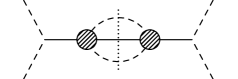
FIG. 4.: Diagrams leading to a branch singularity at $s=M^{2}$. The solid line denotes a massive Higgs boson, the dashed lines stand for massless Goldstone bosons. The cut indicates where the imaginary part is taken.

FIG. 5.: Dyson series with one non-resonant insertion

FIG. 6.: Non-resonant one-loop Feynman diagrams for Goldstone scattering

FIG. 7.: Leading-order (LO) and next-to-leading-order (NLO) results for the Higgs lineshape. The plot shows the $S$-wave amplitude $a_{0}=\frac{1}{16\pi}\int\frac{dt}{s}A(s,t,u)$, using the formulae (35) and (65) for $A(s,t,u)$, respectively. The low-energy limit (21) and the high-energy behavior without renormalization-group improvement are indicated by dotted lines.

FIG. 8.: Deviation from elastic unitarity, shown for the leading-order (LO) and next-to-leading-order (NLO) results for the Higgs lineshape, using the formulae (35) and (65), respectively. The partial wave with spin and weak isospin zero is defined as $a_{00}=\frac{1}{16\pi}\left[\frac{3}{2}\int\frac{dt}{s}A(s,t,u)+\int\frac{dt}{s}A(t,s,u)\right]$. Neglecting multiparticle thresholds, elastic unitarity requires the quantity $|a_{00}-i/2|$ to be equal to $1/2$ if all orders are included. For comparison, we show the NLO result evaluated according to the fixed-width formula (17) [dash-dotted line].

REFERENCES

- [1] B. Lee, C. Quigg and H. Thacker, Phys. Rev. Lett. 38, 883 (1977); Phys. Rev. D16, 1519 (1977); D. Dicus and V. Mathur, Phys. Rev. D7, 3111 (1973).
- [2] S. Glashow, Nucl. Phys. 22, 579 (1961); A. Salam, in: Elementary Particle Theory, ed. N. Svartholm (1968); S. Weinberg, Phys. Rev. Lett. 19, 1264 (1967).
- [3] P.W. Higgs, Phys. Lett. 12, 132 (1964); Phys. Rev. Lett. 13, 508 (1964); Phys. Rev. 145, 1156 (1966); F. Englert and R. Brout, Phys. Rev. Lett. 13, 321 (1964); G.S. Guralnik, C.R. Hagen, and T.W.B. Kibble, Phys. Rev. Lett. 13, 585 (1964); T.W.B. Kibble, Phys. Rev. 155, 1554 (1967).
- [4] C.H. Llewellyn Smith, Phys. Lett. B46, 233 (1973); J.M. Cornwall, D.N. Levin, and G. Tiktopoulos, Phys. Rev. D10, 1145 (1974), E: D11, (1975) 972.
- [5] S. Dawson and S. Willenbrock, Phys. Rev. Lett. 62, 1232 (1989); W. Marciano, G. Valencia, and S. Willenbrock, Phys. Rev. D40, 1725 (1989); L. Durand, J.M. Johnson, and J.L. Lopez, Phys. Rev. Lett. 64, 1215 (1990); Phys. Rev. D45, 3112 (1992); K. Riesselmann, Phys. Rev. D53, 6226 (1996); U. Nierste and K. Riesselmann, Phys. Rev. D53, 6638 (1996).
- [6] A. Blondel, in: Proceedings of Int. Conference on High Energy Physics, Warsaw 1996.
- [7] U. Baur and M. Demarteau, in: Proceedings of the DPF/DPB Summer Study, Snowmass 1996.
- [8] T. Appelquist and C. Bernard, Phys. Rev. D22 (1980) 200; A. Longhitano, Phys. Rev. D22 (1980) 1166; Nucl. Phys. B188 (1981) 118;
- [9] Reviews can be found in: C. Itzykson and J.-B. Zuber, Quantum Field Theory, McGraw-Hill, Singapore (1980); H. Georgi, Weak interactions and modern particle theory, Addison–Wesley, Menlo Park, CA (1984); J.F. Donoghue, E. Golowich, and B.R. Holstein, Dynamics of the Standard Model, Cambridge University Press, Cambridge, UK (1992).
- [10] C.E. Vayonakis, Lett. Nuovo Cim. 17, 383 (1976); M.S. Chanowitz and M.K. Gaillard, Nucl. Phys. B261, 379 (1985); G.J. Gounaris, R. Kögerler, and H. Neufeld, Phys. Rev. D34, 3257(1986); Y.-P. Yao and C.-P. Yuan, ibid. D38, 2237 (1988); J. Bagger and C. Schmidt, ibid. D34, 264 (1990).
- [11] H.-J. He, Y.-P. Kuang, and X.-Y. Li, Phys. Rev. Lett. 69, 2619 (1992); Phys. Lett. B329, 278 (1994); Phys. Rev. D49, 4842 (1994); H.-J. He, Y.-P. Kuang, and C.-P. Yuan, ibid. D51, 6463 (1995); H.-J. He and W.B. Kilgore, ibid. D55, 1515 (1997).
- [12] J. Bagger and C. Schmidt, Phys. Rev. D41, 264 (1990); H. Veltman, Phys. Rev. D41, 2294 (1990); W.B. Kilgore, Phys. Lett. B294, 257 (1992); A. Dobado and J.R. Pelaez, ibid. B329, 469 (1994), E: B335, 554 (1994); J. Horejsi, Preprint PRA-HEP-95/9, hep-ph/9603321; C. Grosse-Knetter and I. Kuss, Z. Phys. C95, 66 (1995); J.F. Donoghue and J. Tandean, Phys. Lett. B361, 69 (1995); T. Torma, Phys. Rev. D54, 2168 (1996); A. Denner and S. Dittmaier, ibid. D54, 4499 (1996); and references therein.
- [13] S. Dawson and G. Valencia, Phys. Lett. B246, 156-162 (1990); Nucl. Phys. B348, 23 (1991); L. Durand and K. Riesselmann, Phys. Rev. D55 (1997) 1533.
- [14] M. Veltman, Act. Phys. Pol. B8 (1977) 475; Nucl. Phys. B123 (1977) 89; P. Sikivie, L. Susskind, M. Voloshin, and V. Zakharov, Nucl. Phys. B173 (1980) 189.
- [15] R. Haag, Phys. Rev. 112 (1958) 669; H. J. Borchers, Nuovo Cim. 25 (1960) 270; D. Ruelle, Helv. Phys. Acta 35 (1962) 34.
- [16] S. Coleman, J. Wess, and B. Zumino, Phys. Rev. 177 (1969) 2239; C. G. Callan, S. Coleman, J. Wess and B. Zumino, Phys. Rev. 177 (1969) 2247; J.M. Cornwall, D.N. Levin, and G. Tiktopoulos, Phys. Rev. D10, 1145 (1974); (E) D11, 972 (1975).
- [17] M. C. Bergère and Y.-M. P. Lam, Phys. Rev. D13 (1976) 3247.
- [18] P. Breitenlohner and D. Maison, Commun. Math. Phys. 52 (1977) 11, 39, 55.
- [19] W. Wetzel, Nucl. Phys. B227, 1 (1983); D.Y. Bardin, A. Leike, T. Riemann, and M. Sachwitz, Phys. Lett. B206, 539 (1988); A. Borelli, M. Consoli, L. Maiani, and R. Sisto, Nucl. Phys. B333, 357 (1990).
- [20] J. Ellis and R. Peccei, eds., Report CERN 86–02 (1986); G. Altarelli et al., eds., Report CERN 89–08 (1989).
- [21] R.G. Stuart, Phys. Lett. B262, 113 (1991); A. Leike, T. Riemann, and J. Rose, Phys. Lett. B273, 513 (1991); T. Riemann, Preprint DESY 97–218, hep-ph/9711305.
- [22] G. Valencia and S. Willenbrock, Phys. Lett. B247, 341 (1990); Phys. Rev. D42, 853 (1990); Phys. Lett. B259, 373 (1991); Phys. Rev. D46, 2247 (1992); T. Binoth and A. Ghinculov, Phys. Lett. B394, 139 (1997); Phys. Rev. D56, 3147 (1997).
- [23] W. Beenakker, G.J. van Oldenborgh, J. Hoogland, and R. Kleiss, Phys. Lett. B376, 136 (1996).
- [24] J. Papavassiliou and A. Pilaftsis, Preprints CERN–TH/97–288, hep-ph/9710380 and CERN–TH/97–293, hep-ph/9710426.
- [25] E.N. Argyres, W. Beenakker, G.J. van Oldenborgh, A. Denner, S. Dittmaier, J. Hoogland, R. Kleiss, C.G. Papadopoulos, and G. Passarino, Phys. Lett. B358, 339 (1995).
- [26] M.H. Seymour, Phys. Lett. B354, 409 (1995).
- [27] M. Lévy, Nuovo Cim. 13, 115 (1959).
- [28] O. Cheyette and M. Gaillard, Phys. Lett. B197, 205 (1987).
- [29] J. Fleischer and F. Jegerlehner, Phys. Rev. D23, 2001 (1981); W.J. Marciano and S. Willenbrock, Phys. Rev. D37, 2509 (1988).
- [30] S. Dawson and S. Willenbrock, Phys. Rev. D40, 2880 (1989);
- [31] K. Riesselmann and S. Willenbrock Phys. Rev. D55, 311 (1997).
- [32] S.N. Gupta, J.M. Johnson, and W.W. Repko, Phys. Rev. D48, 2083 (1993); the expressions for and contain typographical errors, and a term was left out when typewriting the result of .
- [33] A. Ghinculov, Phys. Lett. B337, 137 (1994); (E) B346, 426 (1994); J. van der Bij and A. Ghinculov, Nucl. Phys. B436, 30 (1995).
- [34] L. Durand, P.N. Maher, and K. Riesselmann, Phys. Rev. D48, 1061, 1084 (1993); (E) D52, 553 (1995); A. Frink, B.A. Kniehl, D. Kreimer, and K. Riesselmann, Phys. Rev. D54, 4548 (1996).
- [35] A. Denner, S. Dittmaier, and T. Hahn, Phys. Rev. D56, 117 (1998); A. Denner and T. Hahn, Preprint PSI–PR–97–31, KA–TP–16–1997, hep-ph/9711302.