New String Excitations in the Two-Higgs Standard Model

Abstract

We establish the existence of a static, classically stable string solution in a region of parameters of the generic two-Higgs Standard Model. In an appropriate limit of parameters, the solution reduces to the well-known soliton of the $O(3)$ non-linear sigma model.

The effective theory of electroweak interactions may contain more than the single Higgs doublet of the minimal Standard Model. Theoretical arguments in favour of an extended Higgs sector [1] include supersymmetry and string theory, as well as the possibility of electroweak baryogenesis [2]. Extra Higgs scalars give rise to a richer spectrum of non-perturbative excitations, such as membrane defects [3] and new unstable sphalerons [4]. In this letter we will establish the existence of a new string excitation in the two-Higgs standard model (2HSM), and we will argue that it is stable in a region of parameter space extending into weak coupling.

A systematic way to search for such non-topological excitations has been outlined by two of us in refs. [5, 6]: one considers appropriate limits of parameters so that field space acquires non-trivial topology, thus allowing for topologically-stable solitons. These solitons will generally continue to exist when the parameters are relaxed by a ‘small amount’, so that the degrees of freedom that were frozen or decoupled in the limit affect only slightly the dynamics. A possible exception to this rule occurs when the limiting soliton has zero modes other than its center-of-mass position. Small corrections may lift in this case the degeneracy, and either fix or completely destabilize the excitation. This is exemplified by the Belavin-Polyakov soliton [7], whose arbitrary scale can be fixed by embedding it into a gauged linear sigma model [6].

The purpose of the present letter is to show that one can embed this same soliton as a stable static string defect in the 2HSM. The key observation is that in an appropriate limit of parameters the only relevant dynamical field is the relative SU(2) phase of the two higgses, partially-constrained to lie on a two-sphere $S^{2}$. Our string defects are characterized by the fact that the mapping of the transverse two-dimensional plane onto $S^{2}$ has non-vanishing winding number. In contrast to the previously discussed vortex strings [8] the defects described here carry no net electroweak flux, have no symmetry restoration in their core, and do not exist in the one-Higgs standard model.

The Lagrangian of the 2HSM is ${\cal L}=-{1\over 4}W^{a}_{\mu\nu}W^{a\mu\nu}-{1\over 4}Y_{\mu\nu}Y^{\mu\nu}+|D_{\mu}H_{1}|^{2}+|D_{\mu}H_{2}|^{2}-V(H_{1},H_{2})$, where $W^{a}_{\mu\nu}=\partial_{\mu}W^{a}_{\nu}-\partial_{\nu}W^{a}_{\mu}-g\epsilon^{abc}W^{b}_{\mu}W^{c}_{\nu}$, $Y_{\mu\nu}=\partial_{\mu}Y_{\nu}-\partial_{\nu}Y_{\mu}$. The physical $Z^{0}$ and photon fields are $Z_{\mu}=W^{3}_{\mu}{\rm cos}\theta_{W}-Y_{\mu}{\rm sin}\theta_{W}$ and $A_{\mu}=W^{3}_{\mu}{\rm sin}\theta_{W}+Y_{\mu}{\rm cos}\theta_{W}$ and ${\rm tan}\theta_{W}=g^{\prime}/g$. Both Higgs doublets have hypercharge equal to one, their covariant derivatives are defined by $D_{\mu}H_{1(2)}=\Bigl{(}\partial_{\mu}+{i\over 2}g\tau^{a}W^{a}_{\mu}+{i\over 2}g^{\prime}Y_{\mu}\Bigr{)}H_{1(2)}$, while their potential reads

 

$${{}V(H_{1},H_{2})=\lambda_{1}\Bigl{(}|H_{1}|^{2}-{v_{1}^{2}\over 2}\Bigr{)}^{2}+\lambda_{2}\Bigl{(}|H_{2}|^{2}-{v_{2}^{2}\over 2}\Bigr{)}^{2}}$$

  (1)

This is the most general potential [1] subject to the condition that both CP invariance and a discrete $Z_{2}$ symmetry ($H_{1}\rightarrow-H_{1}$) are only broken softly. The softly broken $Z_{2}$ symmetry is there to suppress unacceptably large flavor-changing neutral currents.

Assuming all $\lambda_{i}$ are positive, the minimum of the potential is, up to gauge transformations, at $<H_{1}>=(0,v_{1}/\sqrt{2})$, $<H_{2}>=e^{i\xi}\;(0,v_{2}/\sqrt{2})$. The perturbative spectrum consists of the electroweak gauge bosons with masses $m_{W}^{2}=g^{2}(v_{1}^{2}+v_{2}^{2})/4$ and $m_{Z}=m_{W}/cos\theta_{W}$ , a charged Higgs scalar $H^{+}$ with mass $m_{H^{+}}^{2}=\lambda_{4}(v_{1}^{2}+v_{2}^{2})/2$, and three neutral scalars, one CP-odd ($A^{0}$) and two CP-even ($h^{0}$ and $H^{0}$) , whose masses depend on the value of $\xi$. The neutral mass matrix simplifies considerably for $\sin\xi\cos\xi=0$. For $\xi=\pi/2$ the neutral masses are $m_{A^{0}}^{2}=\lambda_{5}(v_{1}^{2}+v_{2}^{2})/2$, $m_{h^{0}}^{2}=\zeta-\sqrt{\eta}$ and $m_{H^{0}}^{2}=\zeta+\sqrt{\eta}$, where $\zeta\equiv(\lambda_{1}v_{1}^{2}+\lambda_{2}v_{2}^{2})+(\lambda_{3}+{1\over 4}\lambda_{6})(v_{1}^{2}+v_{2}^{2})$ and $\eta\equiv(\lambda_{1}+\lambda_{3}-{1\over 4}\lambda_{6})^{2}v_{1}^{4}+(\lambda_{2}+\lambda_{3}-{1\over 4}\lambda_{6})^{2}v_{2}^{4}+2v_{1}^{2}v_{2}^{2}\Bigl{(}(\lambda_{3}+{1\over 4}\lambda_{6})^{2}+\lambda_{3}\lambda_{6}-(\lambda_{3}-{1\over 4}\lambda_{6})(\lambda_{1}+\lambda_{2})-\lambda_{1}\lambda_{2}\Bigr{)}$. For $\xi=0$ the masses of $A^{0}$, $h^{0}$ and $H^{0}$ are given by the same expressions with $\lambda_{5}$ and $\lambda_{6}$ interchanged. To simplify the discussion we take $\xi=\pi/2$, $g^{\prime}=\lambda_{3}=\lambda_{4}=0$, and drop the decoupled $U(1)$ gauge field $Y^{\mu}$. We will comment on these assumptions at the end.

Since we are interested in classically-stable static string solutions, we choose the $W_{0}^{a}=0$ gauge and work with static field configurations, so that Gauss’ law is automatically satisfied. Furthermore, for strings stretching in the $x_{3}$ direction we take all fields to be independent of $x_{3}$ and put $W_{3}^{a}=0$. It is easy to verify that stable minima of the ensuing two-dimensional energy functional correspond to stable infinite-string excitations in the original model. Unlike the Nielsen-Olesen-type vortex strings, the finite-energy solutions of interest to us will have $|H_{1(2)}|\neq 0$ everywhere. This fact allows us to use the radial representation of the two doublets, and write them as $H_{1(2)}=F_{1(2)}U_{1(2)}(0\,,\,1)$. $F_{1(2)}$ are two positive functions, while $U_{1(2)}$ are two smooth $SU(2)$ valued functions on the plane. The space of smooth maps from the two-dimensional plane into $SU(2)\equiv S^{3}$ is topologically trivial, and there is no topological obstruction in using the remaining freedom of smooth transverse-space-dependent gauge transformations to set either $U_{1}$ or $U_{2}$ equal to the identity matrix. We will choose $U_{1}=1$ so that the most general Higgs configuration takes the form

$$H_{1}=F_{1}\left(\matrix{0\cr 1\cr}\right)\ \ {\rm and}\ \ H_{2}=F_{2}\,{\rm exp}(-i\Theta{\bf n}\cdot{\bf\tau})\left(\matrix{0\cr 1\cr}\right)$$ (2)

with ${\bf n}\cdot{\bf n}=1$ and ${\bf\tau}$ the Pauli matrices.

In the naive limit $\lambda_{1},\lambda_{2},\lambda_{5}\to\infty$ the $F_{1}$, $F_{2}$ and $\Theta$ freeze at their vacuum values $v_{1}/\sqrt{2}$, $v_{2}/\sqrt{2}$ and $\xi=\pi/2$ respectively. This restricts the Higgs target space to a two-sphere $S^{2}$, parametrized by the unit vector ${\bf n}$. Sending $\lambda_{6}\to 0$ removes the potential of ${\bf n}$. In order to decouple the gauge field we take furthermore the limit $g\to 0$. This is a priori dangerous because it renders the gauge fixing (2) singular. To remedy the situation we must also take $v_{1}\to\infty$ while keeping the gauge-boson mass $m_{W}\sim gv_{1}$ finite. We will see explicitly later on that a finite gauge-boson mass is indeed necessary for our stability analysis.

In the above limit of parameters one is left with an effective O(3) non-linear $\sigma$-model ${\cal L}\sim v_{2}^{2}(\partial_{\mu}{\bf n})^{2}$ describing the dynamics of the unit-vector field ${\bf n}(x)$. The $\sigma$-model has well-known topological solitons in two spatial dimensions [7], characterized by an integer winding number $N$. This is the number of times ${\bf n}(x)$ winds around $S^{2}$ as its argument covers the plane transverse to the defect. It is convenient to parametrize $S^{2}$ through a stereographic projection: $n^{1}+in^{2}=2\Omega/(1+|\Omega|^{2}),n^{3}=(1-|\Omega|^{2})/(1+|\Omega|^{2})$. The $N=1$ string, extending along the $x_{3}$-axis, and with the boundary condition $n^{3}\to 1$ at $\infty$ is then given by

$$\Omega=\rho e^{i\alpha}/(z-z_{0})$$ (3)

where $z\equiv x_{1}+ix_{2}$. The position $z_{0}$, scale $\rho$ and angle $\alpha$ are arbitrary parameters corresponding to soliton zero modes. The value $n^{3}=1$ at $\infty$ will be imposed by the requirement of finiteness of energy once, as we do below, we let $\lambda_{6}\neq 0$.

Following the same steps as in ref. [6], we want now to relax slightly the above limits on the parameters, and study the fate of the solution (3). A simple scaling argument shows that the potential terms tend to shrink the soliton to zero size, while the gauge interactions tend to blow it up. Our task will be to show that in a region of parameter space the soliton is stabilized at some fixed scale $\bar{\rho}$. Our semiclassical analysis looks at first sight incompatible with the strong scalar-coupling limit considered above. To resolve this apparent contradiction, we must redefine the limiting theory in terms of classically-relevant parameters as in [5, 6]. To this end, we rescale the Higgs and gauge fields by $m_{W}/\sqrt{2\lambda_{1}}$, and the transverse space coordinates $x_{j}$ $(j=1,2)$ by $1/m_{W}$. The energy per unit string length takes the form

$${\cal E} = {m_{W}^{2}\over 2\lambda_{1}}\int d^{2}x\;\Biggl{[}F_{2}^{\;2}\Bigl{(}\sin^{2}\Theta(\partial_{i}{\bf n})^{2}+(\partial_{i}\Theta)^{2}\Bigr{)}$$ (4)

$$+ (\partial_{i}F_{1})^{2}+(\partial_{i}F_{2})^{2}+{1\over 2}(F_{1}^{2}-{\tilde{v}}_{1}^{2})^{2}+{\tilde{\lambda}_{2}\over 2}(F_{2}^{\;2}-{\tilde{v}}_{2}^{2})^{2}$$ (5)

$$+ {{\tilde{\lambda}}_{5}\over 2}F_{1}^{\;2}F_{2}^{\;2}\cos^{2}\Theta+{{\tilde{\lambda}}_{6}\over 2}(F_{1}F_{2}n^{3}\sin\Theta-{\tilde{v}}_{1}{\tilde{v}}_{2})^{2}$$ (6)

$$+ {1\over 4}W^{a}_{ij}W^{a}_{ij}+{1\over 4}{\tilde{g}}^{2}(F_{1}^{\;2}+F_{2}^{\;2})W^{a}_{i}W^{a}_{i}-\tilde{g}F_{2}^{\;2}J^{a}_{i}W^{a}_{i}\Biggr{]}$$ (7)

We have defined $\tilde{g}=g/\sqrt{2\lambda_{1}}$, $\tilde{\lambda}_{m}=\lambda_{m}/\lambda_{1}$ for $m=2,5,6$, $\tilde{v}_{1}\equiv\sqrt{2}\cos\beta/\tilde{g}$, $\tilde{v}_{2}\equiv\sqrt{2}\sin\beta/\tilde{g}$, tan$\beta=v_{2}/v_{1}={\tilde{v}}_{2}/{\tilde{v}}_{1}$, and the current $J^{a}_{i}=n^{a}\partial_{i}\Theta+\sin^{2}\Theta\epsilon^{abc}n^{b}\partial_{i}n^{c}+\sin\Theta\cos\Theta\partial_{i}n^{a}$. We have kept the same notation for the rescaled coordinates and fields, as well as for the field strength $W^{a}_{ij}$ which is defined as previously but with the gauge coupling replaced by ${\tilde{g}}$.

Since we will keep $m_{W}$ different from zero in the limiting theory, we can use it to fix the length and mass scales by setting from now on $m_{W}=1$. We may, furthermore, treat $\lambda_{1}$ as the semi-classical expansion parameter, which we will take sufficiently small so as to justify our semiclassical treatment. This leaves us with six classically-relevant parameters: $\tilde{v}_{1}$, $\tilde{v}_{2}$, $\tilde{\lambda}_{2}$, $\tilde{\lambda}_{5}$, $\tilde{\lambda}_{6}$ and $\tilde{g}$. The limiting theory of interest can now be defined more precisely as follows:

$$\tilde{v}_{1},\tilde{\lambda}_{2}\to\infty;\;\tilde{v}_{2},\tilde{\lambda}_{5}\not=0\ \ {\rm fixed};\;\tilde{\lambda}_{6}\tilde{v}_{1}^{2},\tilde{g}\sim\beta\;\to 0.$$ (8)

This looks different from our original naive limit, but has the same dynamical effects. The first set of conditions freeze indeed $F_{1}$, $F_{2}$ and $\Theta$ to their vacuum values, so that the only dynamically-accessible Higgs degree of freedom is the field ${\bf n}(x)$, which parametrizes a two-sphere of non-zero radius. The second set of conditions decouples the gauge field, and ensures that the dynamics of $\bf n$ is described by the usual $O(3)$ non-linear $\sigma$-model, without any additional potential term. The energy functional

$${\cal E}_{(0)}={{\tilde{v}_{2}}^{2}\over 2{\lambda_{1}}}\int d^{2}x\;(\partial_{i}{\bf n})^{2}\ ,$$ (9)

in this limit, admits the Belavin-Polyakov soliton as a (marginally-stable) solution.

Relaxing slightly the limit (8) will introduce a potential, unfreeze the “heavy Higgs modes” $F_{1}-\tilde{v}_{1}\equiv f_{1}$, $F_{2}-\tilde{v}_{2}\equiv f_{2}$ and $\Theta-\pi/2\equiv\theta$, and couple weakly the gauge field $W_{i}^{a}$ to the “light Higgs mode” $\bf n$. These effects can be summarized by a classical (non-local) effective-energy functional [6],

$${\cal E}_{\rm eff} = {\cal E}_{(0)}+{{\tilde{v}_{2}}^{2}\over 4\lambda_{1}}\;\int d^{2}x\;\Biggl{[}\;{\tilde{\lambda}_{6}}{\tilde{v}_{1}}^{2}(n^{3}-1)^{2}-{(\partial_{i}{\bf n}\cdot\partial_{i}{\bf n})^{2}\over{\tilde{\lambda}_{2}}{\tilde{v}_{2}}^{2}}$$ (11)

$$+{\tilde{g}}^{2}{\tilde{v}_{2}}^{2}\int d^{2}y\;j^{a}_{k}(x)G_{ki}(x-y)j^{a}_{i}(y)\;\Biggr{]}+...\ ,$$

where $j^{a}_{k}\equiv\epsilon^{abc}n^{b}\partial_{k}n^{c}$, and $G_{ki}$ is the two-dimensional massive Green function satisfying $(\delta_{jk}\Delta-\partial_{j}\partial_{k}-\delta_{jk})G_{ki}=\delta(\vec{x}-\vec{y})\delta_{ji}$, and given by

$$G_{ki}=-{1\over{(2\pi)^{2}}}\int d^{2}p{{\delta_{ki}+p_{k}p_{i}}\over{\vec{p}^{2}+1}}e^{i\vec{p}\cdot(\vec{x}-\vec{y})}\ .$$ (12)

The first correction in (11) is a potential term. The second and the third come from the exchange of a heavy (radial) mode $f_{2}$ and of a vector boson, respectively. All three are small compared to ${\cal E}_{(0)}$, at least in the range of scales $\rho\sim 1$ that will interest us.

A series of comments on the above energy functional are here in order. First, ${\cal E}_{\rm eff}$ contains an infinite series of terms which come from integrating out classically the heavy Higgs modes and the vector bosons. Inspection of (7) shows that all higher tree diagrams contain extra heavy propagators and/or extra powers of weak couplings. We can ensure that such corrections are indeed subleading by insisting, for instance, that all three heavy Higgs masses be comparable. Secondly, had we set $m_{W}=0$, the gauge-boson exchange diagram would have been IR divergent for configurations with a simple power decay at infinity like (3). A consistent stability analysis would thus be impossible in this case. Finally we should point out that Skyrme-like and potential terms have been used to stabilize the Belavin-Polyakov soliton in the past [9]. The difference is that in our case the non-local and non-renormalizable effective action (11) was derived from the classical field equations of the (renormalizable) 2HSM.

Following [6], we can look for a stable solution of (11) by minimizing the correction terms with respect to the collective coordinates of the zeroth-order solution (3). Since ${\cal E}_{\rm eff}$ is independent of the center-of-mass position and of the U(1) angle $\alpha$, only the size $\rho$ of the soliton is important. The current $j^{a}_{i}$ for the Belavin-Polyakov soliton is $j^{a}_{i}=\epsilon_{ij}\partial_{j}\phi^{a}$, where $\phi^{1}+i\phi^{2}=2\rho(x_{1}-ix_{2})/(r^{2}+\rho^{2})$ and $\phi^{3}=-2\rho^{2}/(r^{2}+\rho^{2})$. A straightforward calculation then gives:

$${{\delta{\cal E}_{\rm eff}(\rho)}\over c}=a\rho^{2}-{b\over{\rho^{2}}}-\int_{0}^{\infty}dz{{z^{3}({K_{1}^{2}(z)+K_{0}^{2}(z)})}\over{(z^{2}/\rho^{2})+1}}$$ (13)

where $K_{0},K_{1}$ are the modified Bessel functions, $\delta{\cal E}_{\rm eff}={\cal E}_{\rm eff}-{\cal E}_{(0)}$, and we have defined the constants
$a\equiv{\tilde{\lambda}_{6}\tilde{v}_{1}^{2}}/{2\tilde{g}^{2}\tilde{v}_{2}^{2}}\;,\;b\equiv 8/{3\tilde{\lambda}_{2}\tilde{g}^{2}\tilde{v}_{2}^{4}}\;,\;c\equiv 2\pi\tilde{g}^{2}\tilde{v}_{2}^{4}/\lambda_{1}$.
The shape of $\delta{\cal E}_{\rm eff}(\rho)$, for different values of the parameters $a$ and $b$, was analyzed numerically. The results are given in Figure 1. At every point below the thick curve the energy has a local minimum, corresponding to a classically-stable soliton of size $\rho=\bar{\rho}(a,b)$.

FIG. 1.: The region of stability of winding string solitons.

The soliton size stays constant along the thin straight lines, as shown in the figure in units of $1/m_{W}$. The assumptions that justified our perturbative treatment, and in particular the condition ${\bar{\rho}}\sim 1$, are satisfied in a large part of the stability region. The validity of our analysis was confirmed independently by a numerical minimization of the energy functional of the 2HSM. We use, in an obvious notation, the most general axially symmetric ansatz

$$H_{1} = \left(\matrix{0\cr h\cr}\right),\;H_{2}=i\left(\matrix{e^{i\phi}f\cr h_{1}+ih_{2}\cr}\right),\;{\bf W}^{3}=W^{3}_{r}{\bf e}_{r}+W^{3}_{\phi}{\bf e}_{\phi}$$ (14)

$${\bf W}^{+} = {1\over\sqrt{2}}e^{i\phi}\bigl{(}(W_{r1}+iW_{r2}){\bf e}_{r}+(W_{\phi 1}+iW_{\phi 2}){\bf e}_{\phi}\bigr{)}$$ (15)

where ${\bf W}^{+}\equiv({\bf W}^{1}-i{\bf W}^{2})/\sqrt{2}$. The $\phi$-dependence is shown explicitly and the ten real unknown functions depend only on $r$.

Figure 2 shows the profile of the solution for $g=0.2$, $v_{2}/v_{1}=0.3$, $\lambda_{1}=0.5$, $\lambda_{2}=20.0$, $\lambda_{5}=1.0$ and $\lambda_{6}=0.0001$ (corresponding to the point A of Figure 1) and with tension ${\cal E}=31.24\pi m_{W}^{2}$. We did not plot neither $h(r)$ which is essentially equal to 6.7728 everywhere, nor $h_{2}$, $W_{r1}$, $W_{\phi 2}$, $W^{3}_{r}$ which to this accuracy are zero. As promised and contrary to what happens for Nielsen-Olesen strings, the magnitudes of the Higgs fields are everywhere non zero. Also, $\Theta\simeq\pi/2$ at all points.

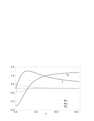
FIG. 2.: The profile of a stable string.

Let us comment briefly on the parameters which were not relaxed from zero in this discussion. From the analysis in [6] we expect that turning on $g^{\prime}$ will favour larger soliton radii, without affecting our qualitative conclusions. The U(1) gauge interactions may even suffice by themselves to stabilize the soliton against shrinking. Similarly, turning on $\lambda_{3}$ should not affect significantly the discussion. Turning on $\lambda_{4}$ on the other hand, to render $H^{+}$ massive, presents a technical difficulty, because the corresponding potential term, evaluated for the zeroth-order soliton, diverges. The divergence is due to the slow approach of $n^{3}$ to its vacuum value at large distances. Although we don’t expect this effect to be physically-significant, our minimization procedure would have to be modified in this case and one must check numerically whether $H^{+}$ can be made heavy enough to comply with experimental bounds. It is on the other hand a welcome fact of our analysis that $\tilde{\lambda}_{5}$ need not be large for stable strings to exist, and that $\tilde{\lambda}_{6}$ is favoured to be small. Realistic values of the CP violation parameter in the Higgs sector, which is proportional to the difference $\tilde{\lambda}_{5}-\tilde{\lambda}_{6}$ [1], may be consistent with string stability even if $\xi$ cannot be relaxed to very small values. Thus, there is no a priori indication that the experimental limits on the parameters of the 2HSM [1] are incompatible with the existence of our defects, but this must be decided ultimately by a numerical analysis of the stability region [10]. The possible accelerator and/or cosmological implications of these solitons may of course depend sensitively on these results.

Finally, having an $S^{2}$ target space in the effective theory suggests that one should also search for stable localized solitons classified by the Hopf index $\pi_{3}(S^{2})$ [11]. The analytic methods of this paper are not however applicable because the zeroth order sigma model lagrangian does not admit such Hopf solutions.

Aknowledgements This research was supported in part by the EU grants CHRX-CT94-0621 and CHRX-CT93-0340, as well as by the Greek General Secretariat of Research and Technology grant 95E$\Delta$1759. We thank the referee for a useful email exchange.

REFERENCES

- [1] J. Gunion, H. Haber, G. Kane and S. Dawson, The Higgs Hunter’s Guide, Addison-Wesley Pub. Co. (1990), and references therein.
- [2] A.I. Bochkarev, S.V. Kuzmin and M.E. Shaposhnikov, Phys. Lett. 244B, 275 (1990) and Phys. Rev. D43, 369 (1991); N. Turok and J. Zadrozny, Phys. Rev. Lett. 65, 2331 (1990); L. McLerran, M. Shaposhnikov, N. Turok and M. Voloshin, Phys. Lett. 256B, 451 (1991).
- [3] C. Bachas and T.N. Tomaras, Phys. Rev. Lett. 76, 356 (1996); G. Dvali, Z. Tavartkiladze and J. Nanobashvili, Phys. Lett. 352B, 214 (1995); A. Riotto and Ola Tornkvist, Phys. Rev. D56, 3917 (1997).
- [4] C. Bachas, P. Tinyakov and T.N. Tomaras, Phys. Lett. B385, 237 (1996).
- [5] C. Bachas and T.N. Tomaras, Nucl. Phys. B428, 209 (1994).
- [6] C. Bachas and T.N. Tomaras, Phys. Rev. D51, R5356 (1995).
- [7] A.A. Belavin and A.M. Polyakov, Pis’ma Zh. Eksp. Teor. Fiz. 22, 503 (1975) [JETP Lett. 22, 245 (1975)].
- [8] Y. Nambu, Nucl. Phys. B130, 505 (1977); T. Vachaspati, Phys. Rev. Lett. 68, 1977 (1992) and Nucl. Phys. B397, 648 (1993); T. Vachaspati and M. Barriola, Phys. Rev. Lett. 69, 1867 (1992); L. Perivolaropoulos, Phys. Lett. 316B, 528 (1993); G. Dvali and G. Senjanovic, Phys. Rev. Lett. 71, 2376 (1993); M. James, T. Vachaspati and L. Perivolaropoulos, Phys. Rev. D46, R5232 (1992) and Nucl. Phys. B395, 534 (1993); M. Earnshaw and M. James, Phys. Rev. D48, 5818 (1993).
- [9] R.A. Leese, R. Peyrard and W.J. Zakrzewski, Nonlinearity 3, 773 (1990).
- [10] T.N. Tomaras, in progres.
- [11] H.J. de Vega, Phys. Rev. D18, 2945 (1977); J. Gladikowski and M. Hellmund, Phys. Rev. D56, 5194 (1997); L. Faddeev and A.J. Niemi, hep-th/9610193.