One-Loop Corrections and All Order Factorization
In Deeply Virtual Compton Scattering

Abstract

We calculate the one-loop corrections to a general off-forward deeply-virtual Compton process at leading twist for both parton helicity-dependent and independent cases. We show that the infrared divergences can be factorized entirely into off-forward parton distributions, even when one of the two photons is onshell. We argue that this property persists to all orders in perturbation theory. We obtain the next-to-leading order Wilson coefficients for the general leading-twist expansion of the product of two electromagnetic currents in the $\overline{\rm MS}$ scheme.

I introduction

Photons, real or virtual, are known to be clean probes of the internal structure of the nucleon. In deep inelastic scattering (DIS), the cross sections for absorption of highly-virtual photons were the first to reveal the internal quark structure of nucleons. The parton distributions extracted from these cross sections contain important structural information and seriously challenge our understanding nonperturbative quantum chromodynamics (QCD). Elastic absorption of virtual photons can be used to measure the electromagnetic form factors of the nucleon. At low virtuality, these form factors give us direct information about the sizes and magnetic moments of nucleons. At high virtuality, they are sensitive to the leading-twist light-cone wavefunctions. More recently, real photon elastic scattering at low energy has been used to extract the electromagnetic polarizablities of nucleons.

In a recent paper, one of us introduced deeply-virtual Compton scattering (DVCS) as a probe to a novel class of “off-forward” parton distributions (OFPD’s) [1]. DVCS is a process in which a highly virtual photon (with virtuality $Q^{2}>\!\!>\Lambda_{\rm QCD}^{2}$) scatters on a nucleon target (polarized or unpolarized), producing an exclusive final state consisting of a high-energy real photon and a slightly recoiled nucleon. With the virtual photon in the Bjorken limit, a QCD analysis shows that the scattering is dominated by the simple mechanism in which a quark (antiquark) in the initial nucleon absorbs the virtual photon, immediately radiates a real one, and falls back to form the recoiled nucleon.

Several interesting theoretical papers have since appeared in the literature, which studied the DVCS process further. In Ref. [2], the single-quark scattering was recalculated using a different, but equivalent definition of the parton distributions. The evolution equations of the distributions were derived and some general aspects of factorization were discussed. In Ref. [3], the evolution equations for OFPD’s were derived and the leading-twist DVCS cross sections were calculated at order $\alpha_{s}^{0}$. Some past and recent studies of OFPD’s can be found in [5]. In Ref. [4], estimates of these cross sections were made at COMPASS and TJNAF energies. In Ref. [6], the DVCS process was considered as a limit of unequal mass Compton scattering, which was studied from the point of view of the operator product expansion. Some early studies of unequal mass Compton processes can be found in Refs. [7, 8]. In Ref. [9], a number of suggestions were made to test the leading twist dominance in DVCS at finite $Q^{2}$. In a Rapid Communication paper, the present authors studied ${\cal O}(\alpha_{s})$ corrections to DVCS for the parton helicity-independent case[10]. In Refs. [11, 12], the same issue was investigated from different perspectives. The present paper is an expanded presentation of our results in Ref. [10].

The main motivation for the present study is to see if the theoretical basis for the DVCS process is up to par with other well-known perturbative QCD processes. More explicitly, we discuss the existence of a factorization theorem for this process. For general two virtual photon processes in the Bjorken limit, the factorizability is suggested by studies of deep inelastic scattering. In the case of DVCS, where one of the photons is onshell, the situation could be different. Potential infrared problems can arise because of the additional light-like vector in this special kinematic limit. However, it is believed that these complications will not ruin the factorization properties [3].

To see factorization at work, it is instructive to work out one-loop examples. We will do this explicitly in section III. For consistency, we consider the unphysical process of DVCS on onshell quark and gluon “targets.” To ensure gauge invariance, we regularize the infrared divergences by going to $d=4+\epsilon$ dimensions. For completeness we have considered both the symmetric and antisymmetric parts of the amplitudes, which are related to helicity-independent and dependent parton distributions, respectively. The only omission is the gluon helicity flip amplitude, which will be discussed in Ref. [13]. As expected, our result contains collinear infrared divergences which can be interpreted as the one-loop perturbative parton distributions, as we will show in Section IV. This property is independent of the special kinematic limit of DVCS.

A general proof of the DVCS factorization was first given by Radyushkin in his approach based on $\alpha$-representation [2]. In this paper, we give an alternative proof using the tools developed by Libby, Sterman, Collins and others [14]. According to these, one can represent the infrared sensitive contributions in a generic Feynman diagram with reduced diagrams. These reduced diagrams have intuitive physical significance and are easy to identify. General power counting rules can be used to select leading reduced diagrams in a process. A recent application of the method can be found in Ref.[15]. We show in Section V that the leading reduced diagrams for DVCS do not contain any soft divergences and are in fact exactly the same as those present when the final state photon is deeply virtual. The collinear divergences in the reduced diagrams can be attributed to those of OFPD’s when calculated in perturbation theory. Therefore we conclude that factorization for DVCS is in the same footing as other well-known examples like deep inelastic scattering.

The factorization property of the general two virtual photon process can be summarized beautifully in terms of Wilson’s operator product expansion. This expansion requires operators with total derivatives [6, 7, 8] to describe the off-forward nature of the process. It is well-known that these derivative operators contribute to the wavefunctions of mesons [16]. In section VI, we convert our one-loop results into Wilson coefficients of the twist-two operators in the $\overline{\rm MS}$ scheme. Together with the two-loop anomolous dimensions of these operators, they provide the necessary ingredients for calculating DVCS at the next-to-leading order.

We summarize and discuss our results in Section VII.

II Kinematics and Parton distributions

Although our ultimate interest is in deeply virtual Compton scattering, we start by considering a general Compton process involving two offshell photons with different virtualities. This and a suitable choice of kinematic variables allows us to exploit the full symmetry of the problem. In the general Compton process, a virtual photon of momentum $q+\Delta/2$ is absorbed by a hadron of momentum $P-\Delta/2$, which then emitts a virtual photon with momentum $q-\Delta/2$ and recoils with momentum $P+{\Delta/2}$. The three independent external momenta can be expanded in terms of the light-cone vectors

$$p^{\mu} = \left(p^{+},0,0,p^{+}\right)\ ,$$ (1)

$$n^{\mu} = {1\over{2p^{+}}}\left(1,0,0,-1\right)\ ,$$ (2)

where the 3-direction is chosen as the direction of the average hadron momentum ($P$), and two transverse vectors. In an expansion, we call the coefficient of $p^{\mu}$ the + component and that of $n^{\mu}$ the $-$ component. Thus we write

$$P^{\mu} = p^{\mu}+{M^{2}-{t/4}\over 2}n^{\mu}\ ,$$ (3)

$$q^{\mu} = -\zeta p^{\mu}+{Q^{2}\over{2\zeta}}n^{\mu}\ ,$$ (4)

$$\Delta^{\mu} = -2\xi p^{\mu}+\xi(M^{2}-t/4)n^{\mu}+\Delta_{T}^{\mu}\ ,$$ (5)

where $M$ is the hadron mass (which is taken to be the same for the initial and final hadrons), $t=\Delta^{2}$, $Q^{2}$ is the virtuality of $q^{\mu}$, $\xi$ is a measure of the difference of the virtualities of the two external photons, $\zeta$ is defined as

$$\zeta={Q^{2}\over{2x_{B}(M^{2}-t/4)}}\left(-1+\sqrt{1+{4x_{B}^{2}(M^{2}-t/4)\over Q^{2}}}\right),$$ (6)

and $\Delta_{T}^{\mu}$ is a vector in the transverse directions which has squared length $-t\left(1-{\xi^{2}}\right)-4\xi^{2}M^{2}$. We have also introduced $x_{B}={Q^{2}/(2P\cdot q)}$, the analogue of the Bjorken scaling variable in this off-forward process. We note that these expressions limit the range of $\xi$ to

$$\xi^{2}\leq{-t\over-t+4M^{2}}\ ,$$ (7)

for fixed $t$, or the range of $t$ to

$$-t\geq{4\xi^{2}M^{2}\over 1-\xi^{2}}\ ,$$ (8)

for fixed $\xi$.

In the Bjorken limit, these expressions simplify considerably. Since we consider only the leading twist in this paper, we may neglect all but the $+$ components of $P^{\mu}$ and $\Delta^{\mu}$ (in order to form large scalars, one must dot the $+$ component of a vector with the $-$ component of $q$). Hence, in the limit $Q^{2}\rightarrow\infty$ ($t$ remaining finite), we may write

$$P^{\mu}\sim p^{\mu}\ ,$$ (9)

$$q^{\mu}\sim-x_{B}p^{\mu}+{Q^{2}\over 2x_{B}}n^{\mu}\ ,$$ (10)

$$\Delta^{\mu}\sim-2\xi p^{\mu}\ .$$ (11)

Here, we note that the external invariants have been reduced from six to three by enforcing kinematics and taking the Bjorken limit. We express these three scalars in terms of one mass scale, $Q^{2}$, and two dimensionless parameters, $x_{B}$ and $\xi$. When we introduce the parton distributions, our expressions will also involve the parton light-cone momentum variable $x$. Hence, the final result will be expressed as algebraic functions of $x_{B}$, $x$, and $\xi$ multiplied by the appropriate power of $Q^{2}$.

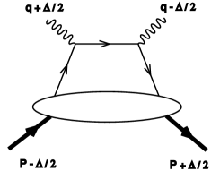
FIG. 1.: The handbag diagram for the general two photon process.

Our goal is to factorize the short and long distance physics of the Compton amplitude in the Bjorken limit,

$$T^{\mu\nu}=i\int d^{\,4}z\,e^{\,iq\cdot z}\left\langle P+{\Delta\over 2}\left|TJ^{\nu}\left({z\over 2}\right)J^{\mu}\left(-{z\over 2}\right)\right|P-{\Delta\over 2}\right\rangle\ ,$$ (12)

where $J^{\mu}=\sum_{q}e_{q}\bar{\psi_{q}}\gamma^{\mu}\psi_{q}$ is the electromagnetic current and $\psi_{q}$ is the bare quark field of flavor $q$ and charge $e_{q}$. The simplest Feynman diagram for this process is shown in Fig. 1, where a quark comes out of the nucleon blob, scatters, and rejoins the nucleon blob. While the scattering involves a large momentum transfer and can be calculated in perturbation theory, the nucleon blob with two quark legs is related to the baryon structure and is nonperturbative. For more complicated graphs, as will be discussed throughout this paper, the Compton amplitude can be separated analogously into soft and hard contributions. In the remainder of this section, we will highlight some important aspects of the soft part.

The nonperturbative contribution to the Compton amplitude in Eq. (12) can be expressed in terms of off-forward parton distributions contained in the parton density matrices[3]. For quarks, we call the density matrix $M_{\alpha\beta}$, where $\alpha$ and $\beta$ are Dirac indices, and expand it in terms of the Dirac matrices. At leading twist, $M_{\alpha\beta}$ is just the light-cone correlation function,

$$M^{q}_{\alpha\beta}\left(x,\xi\right) = \int{d\lambda\over 2\pi}e^{-i\lambda x}\left\langle P+{\Delta\over 2}\left|\bar{\psi}^{q}_{\beta}\left({\lambda\over 2}n\right){\rm P}\left\{e^{-ig\int_{-{\lambda\over 2}}^{\lambda\over 2}n\cdot A\left(\zeta n\right)d\zeta}\right\}\psi^{q}_{\alpha}\left(-{\lambda\over 2}n\right)\right|P-{\Delta\over 2}\right\rangle$$ (13)

$$= {1\over 2}F_{q}{\not\!p}_{\alpha\beta}+{1\over 2}\tilde{F}_{q}\left(\gamma_{5}\not\!p\right)_{\alpha\beta}+\cdots,$$ (14)

where the ellipses denote contributions either of higher twist or chiral-odd structure, which do not contribute to the leading process under consideration. The P symbol denotes the path ordering of the exponential, which makes this expression gauge invariant. It is necessary to include this gauge link whenever one is not working in the light-cone gauge ($A^{+}=0$). Multiplying by $\not\!n_{\beta\alpha}$ and $(\not\!n\gamma_{5})_{\beta\alpha}$ and taking traces, we project out the same distributions as considered in [3]:

$$F_{q}(x,\xi) = {1\over 2}\int{d\lambda\over 2\pi}e^{-i\lambda x}\left\langle P+{\Delta\over 2}\left|\bar{\psi}_{q}\left({\lambda\over 2}n\right){\rm P}\{\}\not\!n\psi_{q}\left(-{\lambda\over 2}n\right)\right|P-{\Delta\over 2}\right\rangle\ ,$$ (15)

$$\tilde{F}_{q}(x,\xi) = {1\over 2}\int{d\lambda\over 2\pi}e^{-i\lambda x}\left\langle P+{\Delta\over 2}\left|\bar{\psi}_{q}\left({\lambda\over 2}n\right){\rm P}\{\}\not\!n\gamma_{5}\psi_{q}\left(-{\lambda\over 2}n\right)\right|P-{\Delta\over 2}\right\rangle\ .$$ (16)

We have suppressed the renormalization scale $\mu$ which is always present in defining a parton distribution. We have also suppressed the $t$ dependence because it will not affect most of the discussions in this paper.

At next to leading order, gluons also contribute to the Compton process. Although it is nontrivial to show, the twist-two gluon distributions are contained in the following gauge-invariant light-cone correlations ($\epsilon^{0123}=+1$),

$$G^{\mu\nu\alpha\beta}(x,\xi) = \int{d\lambda\over 2\pi}e^{-i\lambda x}\left\langle P+{\Delta\over 2}\left|F_{a}^{\mu\nu}\left({\lambda\over 2}n\right){\rm P}\left\{e^{-ig\int_{-{\lambda\over 2}}^{\lambda\over 2}n\cdot A(\zeta n)d\zeta}\right\}_{ab}F_{b}^{\alpha\beta}\left(-{\lambda\over 2}n\right)\right|P-{\Delta\over 2}\right\rangle$$ (17)

$$= -xF_{G}(x,\xi)\left(g^{\mu\alpha}p^{\nu}p^{\beta}-g^{\mu\beta}p^{\nu}p^{\alpha}+g^{\nu\beta}p^{\mu}p^{\alpha}-g^{\nu\alpha}p^{\mu}p^{\beta}\right)$$ (19)

$$+ix\tilde{F}_{G}(x,\xi)\left(\epsilon^{\mu\alpha\gamma\delta}p^{\nu}p^{\beta}-\epsilon^{\mu\beta\gamma\delta}p^{\nu}p^{\alpha}+\epsilon^{\nu\beta\gamma\delta}p^{\mu}p^{\alpha}-\epsilon^{\nu\alpha\gamma\delta}p^{\mu}p^{\beta}\right)n_{\gamma}p_{\delta}+\cdots,$$

where the ellipses denote higher twist contributions and an additional twist-two term which involves gluon helicity flip and will not be considered in this paper [13]. Again, $\rm P\{\}$ denotes path ordering (we note that here the gauge link is in the adjoint representation of $SU(3)$). The off-forward gluon distribution functions $F_{G}$ and $\tilde{F}_{G}$ may be isolated by contraction and are

$$F_{G}=-{1\over 2x}\int{d\lambda\over 2\pi}e^{-i\lambda x}\left\langle P+{\Delta\over 2}\left|F_{a}^{\mu\alpha}\left({\lambda\over 2}n\right){\rm P}\left\{\right\}_{ab}F_{b\,\,\alpha}^{\nu}\left(-{\lambda\over 2}n\right)\right|P-{\Delta\over 2}\right\rangle n_{\mu}n_{\nu}\,\ ,$$ (20)

$$\tilde{F}_{G}=-{i\over 2x}\int{d\lambda\over 2\pi}e^{-i\lambda x}\left\langle P+{\Delta\over 2}\left|F_{a}^{\mu\alpha}\left({\lambda\over 2}n\right){\rm P}\left\{\right\}_{ab}\tilde{F}_{b\,\,\alpha}^{\nu}\left(-{\lambda\over 2}n\right)\right|P-{\Delta\over 2}\right\rangle n_{\mu}n_{\nu}\ .$$ (21)

Here, we have defined the dual field strength tensor $\tilde{F}^{\mu\nu}={1\over 2}\epsilon^{\mu\nu\alpha\beta}F_{\alpha\beta}$.

It is easiest to see the connection of the above gluon distributions with the nonperturbative structure arising from Feynman diagrams in the light-cone gauge. In this gauge, the gauge link is just the unit operator in the adjoint representation and field strength tensors with one + index $F^{+\mu}$ simplify to $\partial^{+}A^{\mu}$. Fourier transformation to momentum space yields

$$F_{G} = -{x_{+}x_{-}\over 2x}{1\over\rm VT}\int{d^{4}\ell\over{(2\pi)}^{4}}\delta(x-\ell\cdot n)$$ (23)

$$\times\left\langle P+{\Delta\over 2}\left|TA^{\mu}_{a}\left(\ell+{\Delta\over 2}\right)A^{\nu}_{a}\left(\ell-{\Delta\over 2}\right)\right|P-{\Delta\over 2}\right\rangle g^{\perp}_{\mu\nu}\ ,$$

$$\tilde{F}_{G} = -i{x_{+}x_{-}\over 2x}{1\over\rm VT}\int{d^{4}\ell\over{(2\pi)}^{4}}\delta(x-\ell\cdot n)$$ (25)

$$\times\left\langle P+{\Delta\over 2}\left|TA^{\mu}_{a}\left(\ell+{\Delta\over 2}\right)A^{\nu}_{a}\left(\ell-{\Delta\over 2}\right)\right|P-{\Delta\over 2}\right\rangle\epsilon_{+-\mu\nu}\ ,$$

where we have defined $x_{+}=x+\xi$ and $x_{-}=x-\xi$. VT represents $(2\pi)^{4}\delta^{4}(0)$, the space-time volume of our system. In a factorized calculation of the Compton amplitude involving gluons, the gluonic indices in the hard part will be contracted with the tensor

$${1\over\rm VT}\int{d^{4}\ell\over{(2\pi)}^{4}}\delta(x-\ell\cdot n)\times\left\langle P+{\Delta\over 2}\left|TA^{i}_{a}\left(\ell+{\Delta\over 2}\right)A^{j}_{a}\left(\ell-{\Delta\over 2}\right)\right|P-{\Delta\over 2}\right\rangle$$ (26)

$$=-{x\over x_{+}x_{-}}\left(F_{G}(x)g^{ij}+i\tilde{F}_{G}(x)\epsilon^{+-ij}\right)\ .$$ (27)

In the above definitions, we have assumed that we are working in 3+1 space-time dimensions. However, to regularize the ultraviolet and infrared divergences arising from loop diagrams, it is convenient to generalize them to $d$ dimensions. Let us first consider the quark density matrix in Eq. (8). Because the spinors are kept in 4 dimensions, the first term on the right hand side generalizes to $d$ dimensions without change. The second term, however, involves $\gamma_{5}$ which has no unique extension. Different choices, in the end, define different factorization schemes. If one uses the t’ Hooft-Veltman definition ($\gamma_{5}=i\gamma^{0}\gamma^{1}\gamma^{2}\gamma^{3}$)[17], one usually introduces an extra renormalization constant $Z_{5}$ so that the non-singlet axial currents are conserved. An alternative choice is offered by Chanowitz, Furman, and Hinchcliffe [18], which employs the usual four-dimensional rules

$$\{{\gamma^{\mu},\gamma_{5}\}} = 0~{}~{}~{}~{}~{}~{}~{}~{}~{}~{}~{}~{}~{}~{}~{}~{}~{}~{}~{}~{}\forall\mu\in[0,d]$$ (28)

$${\rm Tr}[\gamma_{5}\gamma^{\alpha}\gamma^{\beta}\gamma^{\gamma}\gamma^{\delta}] = -(4+{\cal O}(\epsilon))\,\,i\epsilon^{\alpha\beta\gamma\delta}\ .$$ (29)

The ambiguity in the second equation does not affect calculations as long as there are no anomalies in the problem. In the case that there is an anomaly, the ambiguity can be fixed by imposing the relevant Ward identities.

We now turn to the gluon density matrix in Eq. (27). $F_{G}(x)$ contains an average over gluon polarizations. To make this consistent with the number of transverse polarization states available to gluons in $d$ dimensions, we multiply this term by $1/(1+\epsilon/2)$. The polarized gluon density is related to the antisymmetric combination of the gluon fields $F^{+1}$ and $F^{+2}$. This does not change after going to $d$ dimensions if the target polarization is kept the same. Hence, we have left that term as it is.

III One-loop compton amplitudes
on quark and gluon “targets”

In this section, we present a one-loop calculation of the general Compton scattering on onshell quark and gluon “targets” in the Bjorken limit. The result will be used in the next section to show that the factorization of soft and hard contributions can be done consistently with the definition of off-forward parton distributions. In particular, this property does not change in the limit of a real final state photon. Our result will also be used to derive a generalized operator product expansion to next-to-leading order. For the convenience of the reader, we are going to spell out some technical details of the one loop calculation. We believe that some of the techniques, like the cancellation of propagators and light-front coordinate integration, will be useful in other contexts.

We begin with an onshell quark “target”. Here, there are two diagrams at leading order (LO) and eight at next-to-leading order (NLO). Half of these diagrams are shown in Fig. 2. The other half will be taken into account by using the crossing symmetry, i.e., the simultaneous replacement of $q\rightarrow-q$ and $\mu\leftrightarrow\nu$. The terms with $x_{B}\rightarrow-x_{B}$ in the following formulas reflect this contribution. Because of time reversal invariance, the Compton amplitude is also an even function of $\xi$, i.e., symmetric under $\xi\rightarrow-\xi$. This symmetry relates the left and right vertex diagrams (Figs. 2c and 2d, respectively) to each other. On the other hand, the quark self-energy diagram and the box diagram are themselves $\xi$-symmetric. This symmetry not only allows us to reduce the number of graphs at NLO from four to three, but also becomes a powerful tool which helps us compute each amplitude, as we illustrate later.

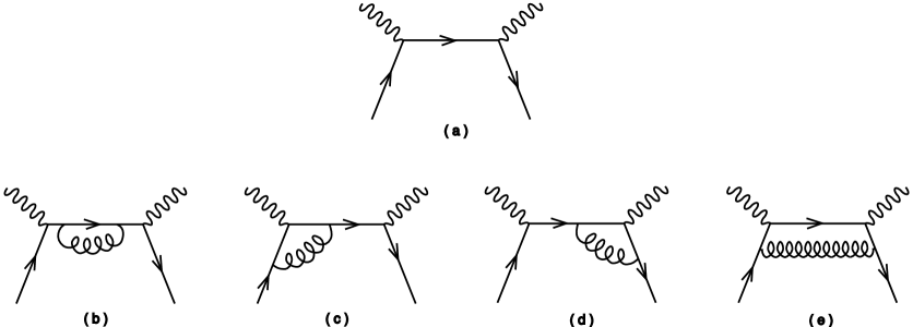
FIG. 2.: Diagrams for Compton scattering on an onshell quark to order $\alpha_{s}$.

Before presenting the details of our calculation, it is necessary to discuss the issues of onshell reduction and ultraviolet divergences. We calculate diagrams in $d$ dimensions and use Feynman’s gauge. As such, we can take the quark target to be massless and take the onshell limit at the beginning of our calculation. In the modified minimal subtraction scheme ($\overline{\rm MS}$), the renormalized single-quark propagator has a residue, $\delta Z$, at the pole ${\not\!p}=0$. According to Lehmann-Symanzik-Zimmerman reduction formula, we calculate the onshell physical matrix element of an operator $\hat{\cal O}_{R}$ as

$$\langle p|\hat{\cal O}_{R}|p\rangle=\lim_{{\not p}\,\rightarrow 0}{\delta Z}\sum_{G}G_{\cal O}\,\,\,\,,$$ (30)

where $G_{\cal O}$ is the set of all amputated connected graphs with one insertion of $\hat{\cal O}_{R}$ in renormalized perturbation theory. The factor $\delta Z$ is infrared divergent for massless quarks and equals $Z_{F}^{-1}$ in the present calculational scheme. Since $J^{\mu}=Z_{F}\bar{\psi}_{R}\gamma^{\mu}\psi_{R}$, all renormalization constants, including the subtraction for the quark self-energy, cancel at one-loop level. Therefore, $T^{\mu\nu}$ for single quark and gluon “targets” can be calculated just from the graphs shown in Fig. 2.

Examining these graphs, we see that the self-energy diagram contains a loop integral with two Feynman denominators, the vertex diagram contains one with three, and the box with four. A one-loop integral with two propagators is straightforward. Difficulties arise, however, with the calculation of three and especially four-propagator integrals. These difficulties may be avoided in this calculation because of several simplifications. Consider first the box diagram. The loop integral is of the form (with momentum routing as shown in Fig. 3)

$$\int{d^{d}k\over{(2\pi)}^{d}}{{{\rm Tr}[\gamma^{\alpha}\left({\not\!k}-\xi\not\!p\right)\gamma^{\nu}\left({\not\!k}+{\not\!q}\right)\gamma^{\mu}\left({\not\!k}+\xi\not\!p\right)\gamma_{\alpha}{\not\!p}(\gamma_{5})]}\over{(k+\xi p)^{2}(k-\xi p)^{2}(k-p)^{2}(k+q)^{2}}}\ ,$$ (31)

where we have replaced $\Delta^{\mu}$ by $-2\xi p^{\mu}$. In order to simplify the integral, we express the trace as a sum of terms which cancel one of the propagators. This can be done because both $k^{2}$ and $2p\cdot k$ can be written as linear combinations of $(k+\xi p)^{2}$ and $(k-\xi p)^{2}$, and the trace vanishes whenever $k^{-}$ and $k_{T}^{2}$ do.

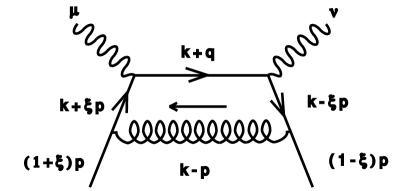
FIG. 3.: The momentum flow in the box diagram

Now that we have shown that a denominator can be cancelled, we have effectively reduced the four-propagator problem to a three-propagator one. Since we have only shown that the numerator will be a linear combination of two different denominators, rather that proportional to one, the four-propagator integral will in general become two three-propagator integrals. However, we may use the $\xi$ symmetry by writing

$$k^{2}={1\over 2} \left(k+\xi p\right)^{2}+(\xi\rightarrow-\xi)\ ,$$ (32)

$$2p\cdot k={1\over 2\xi} \left(k+\xi p\right)^{2}+(\xi\rightarrow-\xi)\ .$$ (33)

In this way, we consider only the $(k+\xi p)^{2}$ cancellation and let the symmetry take care of the rest. We note that the integral we now have is exactly the same (up to numerator differences) as that arising from the right vertex correction. We will see that this basic integral is the only one we must calculate to obtain both the polarized and unpolarized amplitudes for both the quark and gluon contributions (if we forget, for the moment, the simple self-energy diagram). The integral has the form

$$\int{d^{d}k\over{(2\pi)}^{d}}{Numerator\over{[(k-p)^{2}+i\epsilon][(k-{\xi}p)^{2}+i\epsilon][(k+q)^{2}+i\epsilon]}}\,\,.$$ (34)

We have found that this integral is easily done in light-cone coordinates by expanding $k^{\mu}$ in terms of the light cone momenta, $p^{\mu}$ and $n^{\mu}$. We first do the $k^{-}$ integration by contour in the unphysical region of large $x_{B}$, and then the transverse integrations. The $k^{+}$ integration is left until the end. If we write $k^{+}=yp^{+}$, the value of the integral (34) is

$${i\over 16\pi^{2}}\left({Q^{2}\over 4\pi}\right)^{{\epsilon\over 2}}{\Gamma(-{\epsilon\over 2})\over 1-\xi}\left\{\int_{a}^{x_{B}}dy\left({{y-a}\over{x_{B}-a}}\right)^{1+{\epsilon\over 2}}\left(1-{y\over x_{B}}\right)^{{\epsilon\over 2}}N\Big{|}^{a=1}_{a={\xi}}\right\},$$ (35)

where we have defined $N$ according to

$$Numerator\Big{|}_{k^{-}={k_{T}^{2}\over 2p^{+}(y-a)}}=\alpha+\beta k_{T}^{2};$$ (36)

$$N=\beta-{\alpha\over Q^{2}}{{x_{B}(x_{B}-a)}\over{(y-a)(x_{B}-y)}}.$$ (37)

Doing the $y$-integrals requires some care because a delicate cancellation must occur if one is to get finite result, but the treatment is straightforward. After the $\xi$ and crossing symmetries are used, we find the full NLO result for the symmetric quark amplitude

$$T^{(ij)}_{q} = -g^{ij}\sum_{q^{\prime}}e_{q^{\prime}}^{2}\delta_{qq^{\prime}}\left\{{1\over x_{B}-1}-{\alpha_{s}C_{F}\over 4\pi}\left({Q^{2}e^{\gamma_{E}}\over 4\pi\mu^{2}}\right)^{{\epsilon\over 2}}\left\{{3\over{x_{B}-1}}\left(-{2\over\epsilon}+3\right)\right.\right.$$ (42)

$$-{1\over\xi}\left[\left({2\xi\over x_{B}^{2}-1}+{x_{B}+\xi\over 1-\xi^{2}}\right)\left(-{4\over\epsilon}+3-\ln\,\left(1-{\xi\over x_{B}}\right)\right)-3\,{x_{B}-\xi\over 1-\xi^{2}}\right]\ln\left(1-{\xi\over x_{B}}\right)$$

$$\left.+\left[\left({x_{B}+1\over 1-\xi^{2}}+{2\over x_{B}-1}\right)\left(-{4\over\epsilon}+3-\ln\,\left(1-{1\over x_{B}}\right)\right)-3\,{x_{B}-1\over 1-\xi^{2}}\right.\right.$$

$$\left.\left.\left.-{3\over x_{B}-1}\right]\ln\left(1-{1\over x_{B}}\right)\right\}+(x_{B}\rightarrow-x_{B})\right\}$$

and the antisymmetric amplitude

$$T^{[ij]}_{q} = i\epsilon^{\alpha\beta ij}n_{\alpha}p_{\beta}\sum_{q^{\prime}}e_{q^{\prime}}^{2}\delta_{qq^{\prime}}\left\{{1\over x_{B}-1}-{\alpha_{s}C_{F}\over 4\pi}\left({Q^{2}e^{\gamma_{E}}\over 4\pi\mu^{2}}\right)^{{\epsilon\over 2}}\left\{{3\over x_{B}-1}\left(-{2\over\epsilon}+3\right)\right.\right.$$ (46)

$$\left.\left.-\left[\left({2x_{B}\over x_{B}^{2}-1}+{x_{B}+\xi\over 1-\xi^{2}}\right)\left(-{4\over\epsilon}+3-\ln\,\left(1-{\xi\over x_{B}}\right)\right)-{x_{B}-\xi\over 1-\xi^{2}}\right]\ln\left(1-{\xi\over x_{B}}\right)\right.\right.$$

$$+\left[\left({x_{B}+1\over 1-\xi^{2}}+{2\over x_{B}-1}\right)\left(-{4\over\epsilon}+3-\ln\,\left(1-{1\over x_{B}}\right)\right)-{x_{B}-1\over 1-\xi^{2}}\right.$$

$$\left.\left.\left.-{3\over x_{B}-1}\right]\ln\left(1-{1\over x_{B}}\right)\right\}-(x_{B}\rightarrow-x_{B})\right\}\ .$$

Here we have introduced $C_{F}={\rm Tr}[t_{a}t_{a}]={N^{2}_{c}-1\over 2N_{c}}$ in $SU(N_{c})$, where $N_{c}$ is the number of colors. We note that the divergences in these amplitudes are, in fact, infrared divergences since renormalization has removed all ultraviolet singularities. Their presence signals the existence of nonperturbative physics in the process. As mentioned earlier, these divergences will be factorized into nonperturbative matrix elements whose values can be extracted from experiment. We will explicitly show this in the next section. For now, we summarize the results of the gluon piece of the calculation.

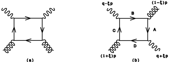
FIG. 4.: Diagrams for gluon Compton scattering at one loop.

There are six graphs which contribute to the LO amplitude for gluon-photon scattering. These six can be reduced to three by reversing the fermion number flow, and one of these can be eliminated by crossing symmetry. The two distinct graphs we must calculate are shown in Fig. 4. The denominator of Fig. 4a is identical to that of the quark box. Again, the numerator is seen to vanish whenever $k^{2}$ and $2p\cdot k$ do, which allows us to cancel one of the propagators exactly as above. Fig. 4b is somewhat more tricky. This diagram is itself symmetric under both crossing and $\xi$ symmetry. Labeling the momenta as shown, we see that under an integral the symmetry $q\rightarrow-q$ is equivalent to $A\leftrightarrow B$ and $C\leftrightarrow D$ and $\xi\rightarrow-\xi$ is equivalent to $B\leftrightarrow D$ and $A\leftrightarrow C$. We also note that here it is possible to represent 1 as a linear combination of Feynman denominators, which guarantees our ability to cancel one. Of course, since 1 does not depend on $q$ or $\xi$, it may be represented in the symmetric form

$$1=-{1\over 2(1-\xi)p\cdot q}A^{2}+(\xi\rightarrow-\xi)+(q\rightarrow-q).$$ (47)

Now it remains only to calculate the trace in a symmetric way and substitute the result into the formulae of the quark calculation. Averaging the gluon polarization for the symmetric amplitude in $d$-dimensions, one finds

$$T_{g}^{(ij)} = -{\alpha_{s}T_{F}\over 2\pi}g^{ij}\left(\sum_{q}e_{q}^{2}\right)\left({Q^{2}e^{\gamma_{E}}\over 4\pi\mu^{2}}\right)^{{\epsilon\over 2}}{1\over 1-\xi^{2}}$$ (51)

$$\left\{\left[\left(1+2x_{B}{x_{B}-1\over 1-\xi^{2}}\right)\left(-{4\over\epsilon}+4-\ln\,\left(1-{1\over x_{B}}\right)\right)-2\right]\ln\left(1-{1\over x_{B}}\right)\right.$$

$$-\left.2x_{B}\left[\left({x_{B}\over 1-\xi^{2}}-{1\over 2\xi}\right)\left(-{4\over\epsilon}+4-\ln\,\left(1-{\xi\over x_{B}}\right)\right)+{1\over\xi}\right]\left(1-{\xi\over x_{B}}\right)\ln\left(1-{\xi\over x_{B}}\right)\right.$$

$$\left.+(x_{B}\rightarrow-x_{B})\right\}\ ,$$

for the symmetric amplitude and

$$T_{g}^{[ij]} = i{\alpha_{s}T_{F}\over 2\pi}\epsilon^{\alpha\beta ij}n_{\alpha}p_{\beta}\left(\sum_{q}e_{q}^{2}\right)\left({Q^{2}e^{\gamma_{E}}\over 4\pi\mu^{2}}\right)^{{\epsilon\over 2}}{1\over 1-\xi^{2}}$$ (55)

$$\left\{\left[\left(1+2{x_{B}-1\over 1-\xi^{2}}\right)\left(-{4\over\epsilon}+4-\ln\,\left(1-{1\over x_{B}}\right)\right)-2\right]\ln\left(1-{1\over x_{B}}\right)\right.$$

$$-\left.2x_{B}\left[{1\over 1-\xi^{2}}\left(-{4\over\epsilon}+4-\ln\,\left(1-{\xi\over x_{B}}\right)\right)\right]\left(1-{\xi\over x_{B}}\right)\ln\left(1-{\xi\over x_{B}}\right)\right.$$

$$-\left.(x_{B}\rightarrow-x_{B})\right\}\ \ ,$$

for the antisymmetric amplitude. We have defined $T_{F}={\rm Tr}[t_{a}t_{b}]={1\over 2}\delta_{ab}$.

IV one-loop factorization
and evolution of Off-forward parton distributions

We now turn to the infrared divergences present in all of the amplitudes. These divergences arise from the regions of loop-mementum integration where some of the internal propagators are near their “mass shells”. In these regions, perturbative calculations are clearly meaningless. The standard procedure of fixing this problem is to factorize the amplitudes into the infrared safe (i.e. devoid of infrared divergences) and infrared divergent pieces, interpreting the latter as nonperturbative QCD quanities. Of course, the factorization procedure has a large degree of arbitrariness. To factorize in a physically interesting way, one usually chooses the nonperturbative objects as the parton distributions in the target, defined in a particular renormalization scheme. In this paper, we consider parton distributions in the $\overline{\rm MS}$ scheme. The goal of this section is to show that all infrared divergences present in the Compton amplitudes can be associated with these distributions.

Since we consider factorization within the framework of perturbation theory, we need to compute the parton distributions in quark and gluon targets in perturbative QCD. At the leading order in $\alpha_{s}$, one has

$$F_{q^{\prime}/q}^{0}(x,\xi)=\delta_{qq^{\prime}}\delta(x-1)\ ,$$ (56)

in an onshell quark $q$. At next-to-leading order, one can calculate directly from the definitions in section II (with the external hadron states replaced with perturbative quark states):

$$F^{1}_{q^{\prime}/q}(x,\xi) = {\alpha_{s}(\mu)\over 2\pi}\delta_{qq^{\prime}}\left({2\over\epsilon}+\ln(\mu^{2}e^{\gamma_{E}}/4\pi\mu_{0}^{2})\right)\left(P(x,\xi)+A\delta(x-1)\right)\ ,$$ (57)

where

$$A=C_{F}\left[{3\over 2}+\int^{x}_{\xi}{dy\over y-x-i\epsilon}+\int^{x}_{-\xi}{dy\over y-x-i\epsilon}\right]\ ,$$ (58)

and

$$P(x,\xi) = C_{F}{x^{2}+1-2\xi^{2}\over(1-x+i\epsilon)(1-\xi^{2})}\ ,~{}~{}~{}~{}~{}~{}~{}~{}~{}~{}x>\xi$$ (59)

$$= C_{F}{x+\xi\over 2\xi(1+\xi)}\left(1+{2\xi\over 1-x+i\epsilon}\right)\ ,~{}~{}~{}~{}~{}-\xi<x<\xi$$ (60)

$$= 0\ ,~{}~{}~{}~{}~{}~{}~{}~{}~{}~{}~{}~{}~{}~{}~{}~{}x<-\xi\ \ .$$ (61)

The quark distributions contain infrared divergences signaled by the presence of the $1/\epsilon$ terms. These divergences reflect the soft physics intrinsic to the parton distributions. $F^{1}_{q^{\prime}/q}$, calculated for the quark target, satisfies the evolution equation derived in Ref. [3] :

$${D_{Q}\,F_{a}(x,\xi)\over D\,\ln Q^{2}}={\alpha_{s}(Q^{2})\over 2\pi}\int_{x}^{1}{dy\over y}P_{ab}\left({x\over y},{\xi\over y}\right)F_{b}(y,\xi),$$ (62)

where $b$ is summed over all parton species and the $P$’s are the off-forward Alterelli-Parisi kernels, or splitting functions. The ‘covariant’ derivative is defined to include $A$, the endpoint contribution in Eq. (57).

We can reexpress the symmetric part of the quark Compton amplitude in terms of the unpolarized, off-forward quark distribution

$$T^{(ij)}_{q} = -g^{ij}\sum_{q^{\prime}}e_{q^{\prime}}^{2}\int^{1}_{-1}dxF_{q^{\prime}/q}(x,\xi)\left\{{1\over x_{B}-x}-{\alpha_{s}C_{F}\over 4\pi}\left\{{9\over{x_{B}-x}}\right.\right.$$ (66)

$$\left.\left.-{x\over\xi}\left[\left({2\xi\over x_{B}^{2}-x^{2}}+{x_{B}+\xi\over x_{+}x_{-}}\right)\left(3-\ln\,\left(1-{\xi\over x_{B}}\right)\right)-3{x_{B}-\xi\over x_{+}x_{-}}\right]\ln\left(1-{\xi\over x_{B}}\right)\right.\right.$$

$$+\left.\left.\left[\left({x_{B}+x\over x_{+}x_{-}}+{2\over x_{B}-x}\right)\left(3-\ln\,\left(1-{x\over x_{B}}\right)\right)-3{x_{B}-x\over x_{+}x_{-}}-{3\over x_{B}-x}\right]\ln\left(1-{x\over x_{B}}\right)\right\}\right.$$

$$\left.+(x_{B}\rightarrow-x_{B})\right\}\ .$$

Analogously, we find that the antisymmetric part of the quark Compton amplitude can be expressed in terms of the polarized off-forward quark distribution

$$T^{[ij]}_{q} = i\epsilon^{\alpha\beta ij}n_{\alpha}p_{\beta}\sum_{q^{\prime}}{e_{q^{\prime}}}^{2}\int^{1}_{-1}dx\tilde{F}_{q^{\prime}/q}(x,\xi)\left\{{1\over x_{B}-x}-{\alpha_{s}C_{F}\over 4\pi}\left\{{9\over x_{B}-x}\right.\right.$$ (70)

$$\left.\left.-\left[\left({2x_{B}\over x_{B}^{2}-x^{2}}+{x_{B}+\xi\over x_{+}x_{-}}\right)\left(3-\ln\,\left(1-{\xi\over x_{B}}\right)\right)-{x_{B}-\xi\over x_{+}x_{-}}\right]\ln\left(1-{\xi\over x_{B}}\right)\right.\right.$$

$$+\left.\left.\left[\left({x_{B}+x\over x_{+}x_{-}}+{2\over x_{B}-x}\right)\left(3-\ln\,\left(1-{x\over x_{B}}\right)\right)-{x_{B}-x\over x_{+}x_{-}}-{3\over x_{B}-x}\right]\ln\left(1-{x\over x_{B}}\right)\right\}\right.$$

$$\left.-(x_{B}\rightarrow-x_{B})\right\}\ .$$

We now turn to Compton scattering on a gluon “target”. Infrared divergent contributions come from the regions where the quarks in the box diagrams are nearly onshell. Therefore, it is natural to associate these divergences with the quark distributions in a gluon target. On the other hand, the finite contributions come from regions where large momenta run through the quark loop. In these regions, the photon has an effective pointlike coupling with the gluons in the target. At leading order, the off-forward gluon distribution in a gluon target is just

$$F_{g/g}^{0}(x,\xi)={1\over 2}(\delta(x-1)-\delta(x+1))\ .$$ (71)

To order $\alpha_{s}$, there are quark partons in the gluon. The corresponding off-forward quark distribution is

$$F^{1}_{q/g}(x,\xi)={\alpha_{s}(\mu)\over 2\pi}\left({2\over\epsilon}+\ln(\mu^{2}e^{\gamma_{E}}/4\pi\mu_{0}^{2})\right)P(x,\xi)\ ,$$ (72)

where for $x>\xi$

$$P(x,\xi)=2T_{F}{x^{2}+(1-x)^{2}-\xi^{2}\over(1-\xi^{2})^{2}}\,\,,$$ (73)

and for $-\xi<x<\xi$

$$P(x,\xi)=T_{F}{(x+\xi)(1-2x+\xi)\over\xi(1+\xi)(1-\xi^{2})}\,\,.$$ (74)

$F^{1}_{q/g}(x,\xi)=0$ for $x<-\xi$.

With the above off-forward distributions, we reexpress the symmetric part of the gluon Compton scattering amplitude

$$T_{g}^{(ij)} = -{\alpha_{s}T_{F}\over 2\pi}g^{ij}\left(\sum_{q}e_{q}^{2}\right)\int^{1}_{-1}dx{x\over x_{+}x_{-}}F_{g/g}(x,\xi)$$ (79)

$$\left\{\left[\left(1+2x_{B}{x_{B}-x\over x_{+}x_{-}}\right)\left(4-\ln\,\left(1-{x\over x_{B}}\right)\right)-2\right]\ln\left(1-{x\over x_{B}}\right)\right.$$

$$-\left.2x_{B}\left[\left({x_{B}\over x_{+}x_{-}}-{1\over 2\xi}\right)\left(4-\ln\,\left(1-{\xi\over x_{B}}\right)\right)+{1\over\xi}\right]\left(1-{\xi\over x_{B}}\right)\ln\left(1-{\xi\over x_{B}}\right)\right\}$$

$$-g^{ij}\sum_{q}{e_{q}^{2}}\int^{1}_{-1}dxF_{q/g}(x,\xi){1\over x_{B}-x}$$

$$+(x_{B}\rightarrow-x_{B})\ .$$

Similarly, we can reexpress the antisymmetric part of the gluon Compton amplitude in terms of helicity-dependent, off-forward quark and gluon distributions

$$T_{g}^{[ij]} = i{\alpha_{s}T_{F}\over 2\pi}\epsilon^{\alpha\beta ij}n_{\alpha}p_{\beta}\left(\sum_{q}e_{q}^{2}\right)\int^{1}_{-1}dx{x\over x_{+}x_{-}}\tilde{F}_{g/g}(x,\xi)$$ (84)

$$\left\{\left[\left(1+2x{x_{B}-x\over x_{+}x_{-}}\right)\left(4-\ln\,\left(1-{x\over x_{B}}\right)\right)-2\right]\ln\left(1-{x\over x_{B}}\right)\right.$$

$$-\left.2x_{B}\left[{x\over x_{+}x_{-}}\left(4-\ln\,\left(1-{\xi\over x_{B}}\right)\right)\right]\left(1-{\xi\over x_{B}}\right)\ln\left(1-{\xi\over x_{B}}\right)\right\}$$

$$+i\epsilon^{\alpha\beta ij}n_{\alpha}p_{\beta}\sum_{q}{e_{q}^{2}}\int^{1}_{-1}dx\tilde{F}_{q/g}(x,\xi){1\over x_{B}-x}$$

$$-(x_{B}\rightarrow-x_{B})$$

We summarize the one-loop Compton amplitude on a target $N$ in the factorization formula

$$T^{ij}_{N} = -g^{ij}\int^{1}_{-1}{dx\over x}\left[\sum_{q}F_{q/N}(x,\xi)C_{q}\left({x\over x_{B}},{\xi\over x_{B}}\right)+F_{g/N}(x,\xi)C_{g}\left({x\over x_{B}},{\xi\over x_{B}}\right)\right]$$ (86)

$$+i\epsilon^{ij\alpha\beta}n_{\alpha}p_{\beta}\int^{1}_{-1}{dx\over x}\left[\sum_{q}\tilde{F}_{q/N}(x,\xi)\tilde{C}_{q}\left({x\over x_{B}},{\xi\over x_{B}}\right)+\tilde{F}_{g/N}(x,\xi)\tilde{C}_{g}\left({x\over x_{B}},{\xi\over x_{B}}\right)\right]\,\,\,,$$

where $C_{q}$, $C_{g}$, $\tilde{C}_{q}$ and $\tilde{C}_{g}$ are shown to order $\alpha_{s}$ in Eqs. (66, 79, 70, 84), respectively. [We emphasize here again that we have neglected the contributions from longitudinally polarized photons and from photon helicity flip. Both effect start at order $\alpha_{s}$.] In the above form, all infrared sensitive contributions have been isolated in the relevant parton distributions, which must be calculated nonperturbatively or measured in experiments. In the DVCS limit $\xi\rightarrow x_{B}$, the coefficient functions remain finite, although they have branch cuts there. This indicates that factorization holds for two-photon amplitudes even when one of the photons is onshell. We will argue in the next section that the above formula, one of the main results of this paper, remains valid to all orders in perturbation theory.

V Factorization of DVCS amplitudes to all orders

In this section, we generalize the one-loop result of the previous section, showing that the factorization formula Eq. (86) is valid in the DVCS limit to all orders in perturbation theory. The one-loop result indicates that all soft divergences - those associated with integration regions where all components of some internal momenta are zero - cancel, whereas all collinear divergences can be factorized into the off-forward parton distributions. To see that this happens also at higher orders in perturbation theory, it is important to understand how the soft cancellation happens in the simplest case.

The self-energy diagram in Fig. 2b does not contain any infrared divergences because the intermediate quark is far offshell. The vertex corrections in Figs. 2c and 2d potentially have infrared divergences, but a simple power counting indicates that these diagrams are in fact infrared convergent. Thus infared divergences appear only in the box diagram. In the region where the gluon momentum $k$ is soft, we can approximate the integral as

$$\sim\int{d^{4}k\over(2\pi)^{4}}{p^{\prime}\cdot p}{1\over p^{\prime}\cdot k}{1\over p\cdot k}{1\over k^{2}}\ ,$$ (87)

where $p$ and $p^{\prime}$ are the momenta of the two external quark lines. On the other hand, the wave function renormalization of an “on-shell” quark, $\delta Z$, also contains infrared divergences. Grouping these divergent terms together, we have the entire soft contribution

$$\sim-{1\over 2}\int{d^{4}k\over(2\pi)^{4}}\left({p^{\mu}\over p\cdot k}-{p^{\prime\mu}\over p^{\prime}\cdot k}\right)^{2}{1\over k^{2}}\ .$$ (88)

In the collinear approximation, $p^{\prime}$ is proportional to $p$ and thus the above integral vanishes.

For higher-order Feynman diagrams, a systematic method of identifying, regrouping and factorizing infrared-sensitive contributions has been developed by Libby, Sterman, Collins, and others [14]. The method essentially consists of the following steps: 1) simplify the Feynman integrals by setting all the soft scales to zero, including the quark masses; 2) identify the regions of loop integration which give rise to infrared divergences; 3) use infrared power counting to find the leading infrared-divergent regions; 4) show that all soft and collinear divergences either cancel or factorize into some nonperturbative quantities. In the remainder of this section, we examine the validity of the factorization formula Eq. (86) in the limit of $x_{B}=\xi$ following the above steps.

In DVCS, the leading contributions come essentially from a massless collinear process in which the external momenta take the form shown in Eq. (6). In this simplified kinematic region, all infrared-sensitive contributions appear as $1/\epsilon$ poles in dimensional regularization. If a contribution contains no infrared divergences, it comes from regions of loop momenta comparable to the hard scale $Q^{2}$, and thus it is insensitive to the soft scales. An infrared divergent contribution must come from the integration regions where some internal propagators are near their mass shells. Since such soft contributions cannot be calculated reliably in perturbative QCD and eventually must be taken into account with nonperturbative matrix elements, one can use any valid infrared regulator to characterize them in perturbative calculations. Thus the collinear massless limit helps to simplify the identification of soft contributions while leaving the truly-perturbative contributions intact.

Infrared divergences appear in a Feynman diagram when some of the external momenta are onshell. The regions of integration producing such contributions can be identified from the Landau equations which are derived by considering the analytical properties of the diagrams as functions of complex external momenta. According to Coleman and Norton [19], these regions can be represented by the so-called reduced diagrams in which offshell lines are shrunk to points and onshell lines are drawn according to their real space-time propagation. We shall argue below that the general leading reduced diagram for DVCS is the one shown in Fig. 5a, in which an incoming virtual photon and an outgoing real one are attached to the hard interaction blob, which in turn is connected to the forward nucleon jet with two collinear quark lines or two physically polarized gluon lines, plus an arbitrary number of longitudinally-polarized collinear gluon lines.

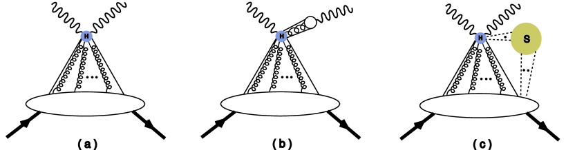
FIG. 5.: General reduced diagrams for the DVCS process.

To decide that a reduced diagram is leading, one can use infrared power counting [20], which is essentially a light-cone dimensional analysis [15]. A simple way to proceed is to consider the mass dimensions of the soft vertices that connect lines with either collinear or soft momenta. Since the dimension of an amplitude is fixed, all soft mass dimensions must be compensated by the hard scale $Q^{2}$. Assuming covariant normalization for the external states ($\langle p|p\rangle=2p^{0}(2\pi)^{3}\delta^{3}(0)$), every external wave function contributes mass dimension $-1$. The collinear quarks and gluons into a soft hadron vertex have effective mass dimensions depending on their polarizations. A Dirac field $\psi$ can be written as a sum of good ($\psi_{+}$) and bad ($\psi_{-}$) components, where $\psi_{\pm}=P_{\pm}\psi$ and $P_{\pm}={1\over 2}\gamma^{\mp}\gamma^{\pm}$. The good (bad) component has effective light-cone mass dimension $1$ ($2$). A vector potential $A^{\mu}$ has light-cone components $A^{+}$, $A^{\perp}$, and $A^{-}$, which have effective mass dimensions 0, 1, and 2, respectively. For the reduced diagram shown in Fig. 5a, the only soft mass dimension comes from the nucleon-quark-gluon blob. Using the above rule, we find it is 0 [$0=2$(physical parton lines $-2$( external nucleon states)]. Because $T^{\mu\nu}$ is dimensionless, the leading reduced diagram contributes at order ${\cal O}(Q^{0})$.

It is somewhat surprising that the leading region is independent of the virtuality of the final state photon as long as the initial photon is deeply virtual. When the final state photon is real, it can have pointlike coupling to quarks as well as extended coupling via its soft wave function, as happens in the case of vector dominance. Thus one has an additional reduced diagram in which a jet of quarks and gluons emerges in the $n^{\mu}$ direction and combines into a real photon long after the hard scattering (Fig 5b). Such a reduced diagram has already been considered in Ref. [15] and is ${\cal O}(Q^{-1})$ by infrared power counting. Indeed, according to the discussion in the previous paragraph, the photon wave function vertex has a soft mass dimension $1=2$ (quark lines) $-1$ (photon state) (recall the dimensionful pion decay constant $f_{\pi}$). A negative hard power $(Q^{-1})$ is needed in $T^{\mu\nu}$ to balance it out.

The power counting involving soft quark and gluon lines is more subtle, and some discussion may be found in Ref. [15]. The result is that any reduced diagram with soft lines connecting the hard scattering blob to the nucleon jet is subleading (Fig. 5c). The situation here is exactly analogous to the case of forward virtual Compton scattering relevant to deep-inelastic scattering as discussed, for instance, by Sterman [20]. A simple example is the vertex correction diagram we already discussed above. When the gluon becomes soft, it has a reduced diagram like Fig. 5c. However, it has no contribution at leading power.

We now come back to the leading reduced diagram shown in Fig. 5a. The collinear gluons with longitudinal polarization connect the hard scattering part and the nucleon jets. These collinear gluons can be factorized using the generalized Ward identities as described in Ref. [14]. Eventually, all collinear gluons can effectively be attached to an eikonal line in the light-cone direction conjuate to the nucleon jet, $n^{\mu}$. Physically, this means that as far as the collinear gluons are concerned, the hard interaction part acts as a jet of particles propagating along $n^{\mu}$. The internal structure of the hard interaction cannot be resolved and thus only the total color charge and momentum of the jet is relevant. The eikonal line together with the physical quarks and gluons and the nucleon jets form the off-forward parton distributions defined in Section II. In the hard scattering, only the total momentum and charge supplied by collinear partons are important. Thus, one can calculate it with incoming physical partons carrying the total momentum and charge of all the collinear longitudinally-polarized gluons. In this way, we have a complete factorization of the soft and hard physics in the DVCS process.

VI Generalized Operator Product Expansion
and Wilson’s Coefficients to the NLO order

The factorization formula in Eq. (86) for the general Compton scattering process can also be examined in the form of an operator product expansion. The OPE was first introduced by Wilson [21] in 1969 and has been used extensively in deep inelastic scattering and other perturbative QCD processes. For the product of two currents separated near the light-cone, the expansion is threefold. Primarily, it is a twist expansion, in which twist-two contributions are leading whereas the higher twist terms are suppressed by powers of $1/Q^{2}$. Each term in the twist expansion contains an infinite number of local operators of the relevant twist. This may be thought of as a kind of Taylor expansion of bilocal operators along the light-cone. Finally, the coefficients of local operators (Wilson coefficients) are themselves expansions in the strong coupling constant. The Wilson coefficients for the unpolarized DIS process were calculated at order $\alpha_{s}$ in the $\overline{\rm MS}$ scheme in [22]. For the polarized case, one can find them in [23].

When considering off-forward processes, the expansion of an operator product must include operators with total derivatives. We call this expansion the generalized OPE. In the remainder of this section, we will recast our factorization formula in its generalized OPE form. In the process, we identify these total derivative operators and obtain their Wilson coefficients to next-to-leading order in $\alpha_{s}$. The final result agrees with the known OPE in the DIS limit ($\xi\rightarrow 0$).

To derive the generalized OPE, we expand $T^{ij}$ in a power series about $x_{B}=\infty$. In this way, we can express the amplitude in terms of moments of the parton disributions rather than the distributions themselves. Eventually, we will relate the moments of parton distributions to the matrix elements of local operators. After the aforementioned expansion, we have

$$T^{ij}=-g^{ij}T_{S}+i\epsilon^{\alpha\beta ij}n_{\alpha}p_{\beta}T_{A}\,\,\,;$$ (89)

$$T_{S}=2\sum_{n\,\rm even=2}^{\infty}\,\,\sum_{m\,\rm even=0}^{\infty}\int^{1}_{-1}{dx\over x}{\left({x\over x_{B}}\right)}^{n}{\left({\xi\over x_{B}}\right)}^{m}\left[\sum_{q}c^{q}_{nm}F_{q}(x,\xi)+c^{g}_{nm}F_{g}(x,\xi)\right]$$ (90)

$$T_{A}=2\sum_{n\,\rm odd=1}^{\infty}\,\,\sum_{m\,\rm even=0}^{\infty}\int^{1}_{-1}{dx\over x}\left({x\over x_{B}}\right)^{n}\left({\xi\over x_{B}}\right)^{m}\left[\sum_{q}\tilde{c}^{q}_{nm}\tilde{F}_{q}(x,\xi)+\tilde{c}^{g}_{nm}\tilde{F}_{g}(x,\xi)\right],$$ (91)

The coefficients for the moments of the quark distributions in the expansion are

$$c_{nm}^{q} = \delta_{m0}-{\alpha_{s}C_{F}\over 4\pi}\left\{\left[9-{8\over n}+{2\over n+1}+4S_{2}(n-1)-4T_{1}^{1}(n-1)\right.\right.$$ (94)

$$\left.-S_{1}(n-1)\left(3+{2\over n}+{2\over n+1}\right)\right]\delta_{m0}+\left[{6n\over m(m+n)}-{1\over(n+m)(n+m+1)}\right.$$

$$\left.\left.+{4\over m}S_{1}(m-1)-2S_{1}(n+m-1)\left({1\over n+m}+{1\over n+m+1}\right)\right](1-\delta_{m0})\right\}\ ,$$

$$\tilde{c}_{nm}^{q} = \delta_{m0}-{\alpha_{s}C_{F}\over 4\pi}\left\{\left[9-{6\over n}+4S_{2}(n-1)-4T_{1}^{1}(n-1)\right.\right.$$ (98)

$$\left.-S_{1}(n-1)\left(3+{2\over n}+{2\over n+1}\right)\right]\delta_{m0}+\left[{6n\over m(n+m)}-{3\over m}+{4\over m}S_{1}(m-1)\right.$$

$$\left.\left.-2S_{1}(n+m-1)\left({1\over n+m}+{1\over n+m+1}\right)\right]\left(1-\delta_{m0}\right)\right\}\ ,$$

where we have introduced

$$S_{j}(n):=\sum_{i=1}^{n}{1\over i^{j}}\ ,$$ (99)

$$T_{j}^{k}(n):=\sum_{i=1}^{n}{S_{j}(i)\over i^{k}}\ .$$ (100)

Notice that the above expansion contains only positive powers of $x$ and $\xi$. This result is not immediately obvious because of the $x_{+}x_{-}$ denominators in the amplitudes. In the case of the gluon distribution functions, we have an additional factor of $x_{+}x_{-}$ in the denominator. Since the final OPE contains only local operators, these factors have to be cancelled in the process of expansion. Indeed, this turns out to be the case and we obtain the coefficients of the positive moments of the gluon distributions

$$c_{nm}^{g} = {\alpha_{s}T_{F}\over 2\pi}\left[{m\over n+m}-{m+2\over n+m+2}-2S_{1}(n+m-1)\left({1\over n+m}-{m+2\over n+m+1}+{m+2\over n+m+2}\right)\right]$$ (101)

$$\tilde{c}_{nm}^{g} = {\alpha_{s}T_{F}\over 2\pi}\left[2+2S_{1}(n+m-1)\right]\left({m+1\over n+m}-{m+2\over n+m+1}\right)\left(1-\delta_{n1}\right)\ .$$ (103)

Having obtained an expansion involving the moments of the distributions, we move toward a general form of the OPE. To this end, we consider the moments of the parton distributions. We begin by observing that for quarks

$$\int^{1}_{-1}dxx^{n-1}F_{q}(x,\xi)={1\over 2}\left\langle P_{f}\left|\bar{\psi}_{q}(0)\stackrel{{\scriptstyle\leftrightarrow}}{{i\partial}}_{\mu_{1}}\cdots\stackrel{{\scriptstyle\leftrightarrow}}{{i\partial}}_{\mu_{n-1}}\gamma_{\mu_{n}}\psi_{q}(0)\right|P_{i}\right\rangle n^{\mu_{1}}\cdots n^{\mu_{n}}$$ (104)

holds in light-cone gauge, where we have defined $\stackrel{{\scriptstyle\leftrightarrow}}{{\partial}}\,={1\over 2}(\stackrel{{\scriptstyle\rightarrow}}{{\partial}}-\stackrel{{\scriptstyle\leftarrow}}{{\partial}})$. The parton distribution depends on $x$ only through the exponential, which allows one to integrate over the $x$ through simple partial integrations. The $\lambda$ integration can then be done trivially. So the moments of the quark distribution can be expressed in terms of the matrix elements of local operators in the light-cone gauge. However, in this gauge, these gauge-dependent local operators are equal to the gauge invariant operators obtained by replacing the partial derivatives in the above expression by covariant derivatives,

$${}_{q}{\cal O}_{\mu_{1}\mu_{2}\cdots\mu_{n}}^{n}=\bar{\psi}(0)\stackrel{{\scriptstyle\leftrightarrow}}{{i\cal D}}_{(\mu_{1}}\cdots\stackrel{{\scriptstyle\leftrightarrow}}{{i\cal D}}_{\mu_{n-1}}\gamma_{\mu_{n})}\psi(0),$$ (105)

where $(\cdots)$ signifies that the indices are symmetrized and the trace has been removed. Thus the moments of the quark distribution functions are just matrix elements of the + components of the above operators between the initial and final hadron states. We also recognize that

$$(n\cdot i\partial)\,\,_{q}{\cal O}_{n}^{+\cdots+}=2\xi{\cal O}_{n}^{+\cdots+}\ .$$ (106)

This prompts us to define

$${}_{q}{\cal O}^{n,m}_{\mu_{1}\mu_{2}\cdots\mu_{n}} = i\partial_{\,(\mu_{1}}\cdots i\partial_{\,\mu_{m}}\bar{\psi}(0)\stackrel{{\scriptstyle\leftrightarrow}}{{i\cal D}}_{\mu_{m+1}}\cdots\stackrel{{\scriptstyle\leftrightarrow}}{{i\cal D}}_{\mu_{n-1}}\gamma_{\mu_{n})}\psi(0)\ ,$$ (107)

$${}_{q}{\tilde{\cal O}}^{n,m}_{\mu_{1}\mu_{2}\cdots\mu_{n}} = i\partial_{\,(\mu_{1}}\cdots i\partial_{\,\mu_{m}}\bar{\psi}(0)\stackrel{{\scriptstyle\leftrightarrow}}{{i\cal D}}_{\mu_{m+1}}\cdots\stackrel{{\scriptstyle\leftrightarrow}}{{i\cal D}}_{\mu_{n-1}}\gamma_{\mu_{n})}\gamma_{5}\psi(0)\ .$$ (108)

$${}_{g}{\cal O}^{n,m}_{\mu_{1}\mu_{2}\cdots\mu_{n}} = i\partial_{\,(\mu_{1}}\cdots i\partial_{\,\mu_{m}}F_{\mu_{m+1}\alpha}(0)\stackrel{{\scriptstyle\leftrightarrow}}{{i\cal D}}_{\mu_{m+2}}\cdots\stackrel{{\scriptstyle\leftrightarrow}}{{i\cal D}}_{\mu_{n-1}}F^{\alpha}_{~{}\mu_{n}}(0)\ ,$$ (109)

$${}_{g}{\tilde{\cal O}}^{n,m}_{\mu_{1}\mu_{2}\cdots\mu_{n}} = i\partial_{\,(\mu_{1}}\cdots i\partial_{\,\mu_{m}}F_{\mu_{m+1}\alpha}(0)\stackrel{{\scriptstyle\leftrightarrow}}{{i\cal D}}_{\mu_{m+2}}\cdots\stackrel{{\scriptstyle\leftrightarrow}}{{i\cal D}}_{\mu_{n-1}}i\tilde{F}^{\alpha}_{~{}\mu_{n}}(0)\ .$$ (110)

After replacing the moments of parton distributions in Eq.(91) with matrix elements of these operators and interpreting the result as an operator relation, we find the following generalized OPE,

$$~{}~{}~{}i\int d^{\,4}z~{}e^{iq\cdot z}~{}TJ^{\,\nu}\left({z\over 2}\right)J^{\,\mu}\left(-{z\over 2}\right)$$ (111)

$$= (-g^{\mu\nu}+\cdots)\sum_{n~{}\rm even=2}^{\infty}\,\,\sum_{m~{}\rm even=0}^{n}\left({2^{n-m}q_{\mu_{1}}\cdots q_{\mu_{n}}\over(Q^{2})^{n}}\right)\sum_{a=q,g}c^{a}_{n-m,m}\,\,{}_{a}{\cal O}_{n,m}^{\mu_{1}\cdots\mu_{n}}$$ (113)

$$+i\epsilon_{\mu\nu\alpha\beta}q^{\alpha}\sum_{n~{}\rm odd=1}^{\infty}\,\,\sum_{m~{}\rm even=0}^{n}\left({2^{n-m}q_{\mu_{2}}\cdots q_{\mu_{n}}\over(Q^{2})^{n}}\right)\sum_{a=q,g}\tilde{c}^{a}_{n-m,m}\,\,{}_{a}\tilde{\cal O}_{n,m}^{\beta\mu_{2}\cdots\mu_{n}}+...$$

It must be pointed out that the generalized OPE does not have a unique form. One can define $x_{B}$ as any dimensionless invariant formed from the external momenta which remains finite in the Bjorken limit and expand the amplitude in inverse powers of this variable. This will lead to a different set of coefficient functions, but the physical content is the same. The choice of which OPE to use is determined by the specifics of the problem at hand.

Of course, the above expression contains only the contributions to leading order in $1/Q^{2}$. Since the operators ${\cal O}_{n,m}$ are symmetrized and traceless, their rank is $n$. The mass dimension of these operators is just the dimension of the fermion fields plus that of the derivatives, or $3+n-1$. Hence these operators are all twist 2. At the next order in $1/Q^{2}$ one has to consider operators of higher twist, which are beyond the scope of this paper.

VII summary and comments

In this paper, we have studied the QCD factorization for deeply virtual Compton scattering explicitly at one loop and then to all orders in perturbation theory. Our conclusion is that DVCS is factorizable in perturbation theory. This statement has the same level of rigor as the ordinary operator production expansion used in deep-inelastic scattering. In fact, assuming the generalized OPE with total derivative operators, DVCS can be recovered by analytically continue $x_{B}$ variable from $x_{B}>1$ region to the point $x_{B}=\xi$. The factorization theorem guarantees that the Compton amplitudes are finite there, although the one-loop calculation indicates that they are not analytic.

We have also computed the coefficient functions to order $\alpha_{s}$ for the generalized OPE including the total derivative operators. For general two photon processes, one has to include the longitudinal photon scattering, which has been done in Ref. [12], and photon-helictity flip amplitude [13]. The scale evolution of total derivative operators can best be studied using conformally-symmetric operators [11]. In fact, it has been known for a long time that at the leading-log level, the operators of same twist and dimension evolve multiplicatively in Gegenbauer polynomial combinations. It is a simple excercise to transform Eq. (113) into this basis.

Note Added: After this work was completed, we learned that the DVCS factorization has also been studied by Collins and Freud [24]. Their arguments and conclusions are similar to ours. We also learned that some aspects of higher-order corrections to DVCS have been considered by Belitsky and Schäfer [25].