BROOKHAVEN NATIONAL LABORATORY   December, 1997 BNL-HET-98/1   
Supersymmetry Signatures at the CERN LHC
Frank E. Paige Physics Department Brookhaven National Laboratory Upton, NY 11973 USA
ABSTRACT These lectures, given at the 1997 TASI Summer School, describe the prospects for discovering supersymmetry (SUSY) and for studying its properties at the Large Hadron Collider (LHC) at CERN. If SUSY exists at a mass scale less than 1–$2\,{\rm TeV}$, then it should be easy to observe characteristic deviations from the Standard Model at the LHC. It is more difficult to determine SUSY masses because in most models there are two missing particles ${\tilde{\chi}_{1}^{0}}$ in every event. However, it is possible to use various kinematic distributions to make precision measurements of combinations of SUSY masses and other quantities related to SUSY physics. In favorable cases such measurements at the LHC can determine the parameters of the underlying SUSY model with good accuracy.
To appear in TASI 97: Supersymmetry, Supergravity and Supercolliders (Boulder, CO, 1997). This manuscript has been authored under contract number DE-AC02-76CH00016 with the U.S. Department of Energy. Accordingly, the U.S. Government retains a non-exclusive, royalty-free license to publish or reproduce the published form of this contribution, or allow others to do so, for U.S. Government purposes.

Supersymmetry Signatures at the CERN LHC

These lectures, given at the 1997 TASI Summer School, describe the prospects for discovering supersymmetry (SUSY) and for studying its properties at the Large Hadron Collider (LHC) at CERN. If SUSY exists at a mass scale less than 1–$2\,{\rm TeV}$, then it should be easy to observe characteristic deviations from the Standard Model at the LHC. It is more difficult to determine SUSY masses because in most models there are two missing particles ${\tilde{\chi}_{1}^{0}}$ in every event. However, it is possible to use various kinematic distributions to make precision measurements of combinations of SUSY masses and other quantities related to SUSY physics. In favorable cases such measurements at the LHC can determine the parameters of the underlying SUSY model with good accuracy.

1 Introduction

The theoretical attractiveness of having supersymmetry (SUSY) at the electroweak scale has been discussed by many authors.^?,? But while SUSY is perhaps the most promising ideas for physics beyond the Standard Model, we will not know if it is a correct idea until SUSY particles are discovered experimentally. LEP might still discover a SUSY particle, but it has already run at $\sqrt{s}=183\,{\rm GeV}$, and its reach will be limited by its maximum energy, probably $\sqrt{s}=193\,{\rm GeV}$. It is less unlikely that LEP might discover a light Higgs boson: the current bound^? of $\sim 77\,{\rm GeV}$ is expected to be improved to $\mathrel{\hbox to0.0pt{\raise 2.20013pt\hbox{$<$}\hss}{\lower 2.20013pt\hbox{$\sim$}}}95\,{\rm GeV}$,^? whereas the upper limit on the mass is $\sim 130\,{\rm GeV}$ in the Minimal Supersymmetric Standard Model^? and $\sim 150\,{\rm GeV}$ more generally.^? Finding a light Higgs would not prove the existence of SUSY, but it would certainly be a strong hint.

The Tevatron has a better chance of finding SUSY particles, particularly from the process^?,?

$$\bar{p}p\to{\tilde{\chi}}_{2}^{0}{\tilde{\chi}}_{1}^{\pm}\to\ell^{+}\ell^{-}\ell^{\pm}\hbox to0.0pt{\hbox to7.95831pt{\hfil/\hfil}\hss}E_{T}\,.$$

This can be sensitive to $M({\tilde{\chi}}_{2}^{0})\approx M({\tilde{\chi}}_{1}^{\pm})\mathrel{\hbox to0.0pt{\raise 2.20013pt\hbox{$<$}\hss}{\lower 2.20013pt\hbox{$\sim$}}}200\,{\rm GeV}$ for some choices of the other parameters, e.g., small $\tan\beta$, given an integrated luminosity of $2\,{\rm fb}^{-1}$ in Run 2 and more in future runs.^? But, like LEP, the Tevatron cannot exclude SUSY at the weak scale.

The decisive test of weak scale SUSY, therefore, must await the Large Hadron Collider (LHC) at CERN. The LHC can detect gluinos and squarks in the MSSM up to $\sim 2\,{\rm TeV}$ with only 10% of its design integrated luminosity per year. Discovering gluinos and squarks in the expected mass range, $\mathrel{\hbox to0.0pt{\raise 2.20013pt\hbox{$<$}\hss}{\lower 2.20013pt\hbox{$\sim$}}}1\,{\rm TeV}$, seems straightforward, since the rates are large and the signals are easy to separate from Standard Model backgrounds. Other SUSY particles can be found from the decays of gluinos and squarks. The difficult problem is not discovering SUSY if it exists but verifying that the new physics is indeed SUSY, separating the various SUSY signals, and interpreting them in terms of the parameters of an underlying SUSY model. This is more difficult for the LHC than for an $e^{+}e^{-}$ machine of sufficient energy, but some progress has been made recently.

The first few sections of these lectures are mainly review. Section 2 reviews the SUSY production cross sections and some basic facts about QCD perturbation theory. Section 3 discusses event generators, which are used to translate production cross sections into experimental signals. Section 4 summarizes the capabilities of ATLAS and CMS, the two main LHC detectors, to detect these signals.

The next sections concentrate on SUSY measurements at the LHC in the context of the minimal supergravity (SUGRA) model,^? although the general results should apply to other models, at least those in which the lightest SUSY particle escapes the detector. Section 5 shows the reach in SUGRA parameter space for various signals and describes how to make a first estimate of the SUSY mass scale. Section 6 describes examples of a recently developed approach to extracting information about SUSY masses and other parameters from LHC data for five specific SUGRA points. Section 7 shows what the resulting errors on the SUGRA parameters would be at these points. Section 8 discusses preliminary results at a SUGRA point with large $\tan\beta$ that has very different properties.

Section 9 discusses the LHC discovery potential for Higgs bosons both in the Standard Model and in the MSSM. Finally, Section 10 draws some conclusions.

2 SUSY Cross Sections

The LHC is a $pp$ collider to be built in the existing LEP tunnel at CERN (the European Laboratory for Particle Physics, located near Geneva, Switzerland) with a center-of-mass energy $\sqrt{s}=14\,{\rm TeV}$ and a luminosity ${\cal L}=10^{33}$–$10^{34}\,{\rm cm^{-2}s^{-1}}$. It will have two major experiments, ATLAS^? and CMS,^? for studying high-$p_{T}$ physics like SUSY. Two smaller experiments — LHC-B for $B$ physics and ALICE and for heavy ion physics — have also been proposed but will not be discussed further here. Construction of both the accelerator and the experiments is expected to be completed in 2005.^?

Fine tuning arguments^? suggest that the SUSY masses should be below about $1\,{\rm TeV}$ if SUSY is relevant to electroweak physics. Then SUSY production at the LHC is dominated by the production of gluinos and squarks. The elementary ${\tilde{g}}$ and ${\tilde{q}}$ cross sections only depend on the color representations and spins of these particles — which of course are fixed by supersymmetry — and on their masses. Thus they are less model dependent than the cross sections for gaugino production, which also depend on couplings determined by the mixing matrices.

Perturbative QCD tells us that inclusive production cross sections can be computed as a power series in the strong coupling coupling $\alpha_{s}(Q)$ evaluated at a scale $Q$ of order the masses involved. For example, the lowest order contribution to the elementary process $gg\to{\tilde{g}}{\tilde{g}}$ is given by^?

$${d\hat{\sigma}\over d\hat{t}} = {9\pi\alpha_{s}^{2}\over 4\hat{s}^{2}}\Biggl{\{}{2(\hat{t}-M^{2})(\hat{u}-M^{2})\over\hat{s}^{2}}+$$

$$\qquad\qquad\left[{(\hat{t}-M^{2})(\hat{u}-M^{2})-2M^{2}(\hat{t}+M^{2})\over(\hat{t}-M^{2})^{2}}+(\hat{t}\leftrightarrow\hat{u})\right]+$$

$$\qquad\qquad{M^{2}(\hat{s}-4M^{2})\over(\hat{t}-M^{2})(\hat{u}-M^{2})}\Biggr{\}}\,,$$

where $\hat{s}$, $\hat{t}$, $\hat{u}$ are usual parton process invariants and $M=M_{\tilde{g}}$ is the only relevant mass in this case. The lowest order cross section for $gg\to{\tilde{q}}\bar{{\tilde{q}}}$ depends on both $M_{\tilde{q}}$ and $M_{\tilde{g}}$. The cross sections for gaugino pair production and associated production depend on the masses and also on couplings which are determined by the chargino and neutralino mixing matrices.

The elementary cross sections are then related to $pp$ cross sections by the QCD-improved parton model, which is based on the impulse approximation for processes with large $Q^{2}$. In the parton model the $pp$ cross section is given by a convolution of the elementary parton-parton cross sections and the appropriate parton distributions, i.e., the probabilities of finding quarks or gluons with given momentum fractions $x_{i}$ in the incoming protons:

$$\sigma=\sum_{ij}\int dx_{1}dx_{2}\,\hat{\sigma}_{ij}f_{i}(x_{1},Q^{2})f_{j}(x_{2},Q^{2})\,.$$

Here $Q^{2}$ is a measure of the scale, e.g. $Q^{2}=p_{T}^{2}+M^{2}$, and $x_{i}$ are the momentum fractions of the incoming partons. By elementary kinematics they satisfy

$$\hat{s}=x_{1}x_{2}s,\quad x_{i}=\sqrt{\hat{s}\over s}e^{\pm\hat{y}}\,,$$

where $\hat{y}$ is the rapidity of the center of mass of the produced system.

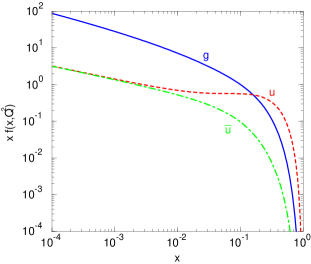
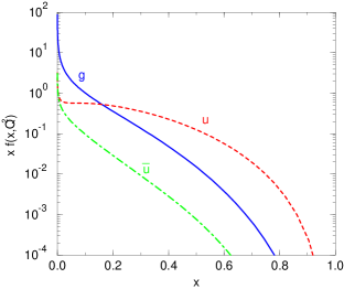
Figure 1: $g$, $u$, and $\bar{u}$ parton distributions $xf(x,Q^{2})$ in the proton vs. $x$ for $Q=100\,{\rm GeV}$ using the CTEQ3L^? parameterization.

Representative parton distributions for $Q=100\,{\rm GeV}$ are shown in Figure 1. Note that

$$x\sim\sqrt{\hat{s}\over s}\mathrel{\hbox to0.0pt{\raise 2.20013pt\hbox{$>$}\hss}{\lower 2.20013pt\hbox{$\sim$}}}{2M_{\tilde{g}}\over\sqrt{s}}\,$$

so that $g(x)$ is large and $gg$ processes dominate the production of squarks and gluinos for most masses of interest.

Figure 2: Soft and collinear singularities both come from gluons attached to external lines, only one of which is shown. Soft singularities come from $p^{2}=m^{2}$ and $k\to 0$; collinear ones come from $p^{2}=k^{2}=0$ and $\theta_{pk}\to 0$. The gluon can be either real or virtual.

The QCD-improved parton model is intuitively plausible, but we must require that it is consistent with higher order perturbation theory. Consider adding one gluon emission or loop. Then after renormalization of ultraviolet divergences in the usual way, individual graphs are found to give a series not in $\alpha_{s}$ but in $\alpha_{s}\ln^{2}Q^{2}$. These logarithms must cancel if perturbation theory is to be usable. There is only one large $Q^{2}$ in the problem, so the logarithms must reflect singularities as the external particles are put on mass shell. There are actually two distinct types of singularities, both well known from QED:

Soft or Infrared Singularities: These arise from a gluon with $k\to 0$ attached to an external line, Figure 2. Then as the external line goes on shell, so does the internal propagator. Soft singularities arise from the divergent multiplicity of soft gluons; the probability of radiating no gluons from an accelerated color charge is zero. The total cross section must be finite — something must happen. Hence the singularities must cancel between processes with different numbers of gluons, i.e., between real and virtual graphs. This can be proven to all orders in perturbation theory for QED.^?,? The situation in QCD is more complicated because the gluons themselves radiate, but the cancelation certainly works in all cases that have been tried.

Collinear or Mass Singularities: These arise from the emission of a hard gluon parallel to a massless parton in the initial state, i.e., $p^{2}=k^{2}=0$ and $k\|p$ in Figure 2 . (There also can be collinear singularities in the final state for differential cross sections.) They do not cancel for initial states like hadrons with limited transverse momenta, but they are universal because they come from on-shell poles.^? Hence they cancel if you calculate one physical process, e.g., ${\tilde{g}}{\tilde{g}}$ production, in terms of another, e.g., deep inelastic scattering. Equivalently, they can be absorbed into universal parton distributions defined by deep inelastic scattering. It is straightforward to verify this at one loop. The general proof is complex because soft and collinear singularities get tangled,^? but the result is believed to be true.

The collinear singularities in the parton distributions lead to a series in $(\alpha_{s}(Q^{2})\ln Q^{2})={\cal O}(1)$. These leading logarithms can be summed to all orders in perturbation theory: Altarelli and Parisi^? matched the operator product expansion to the 1-loop graphs, while Gribov and Lipatov^? and Dokshitser^? studied the origin of the logarithms in perturbation theory directly. The result is that the parton distributions satisfy the DGLAP equations,

$${\partial q_{i}(x,Q^{2})\over\partial Q^{2}} = \displaystyle{\alpha_{s}(Q^{2})\over 2\pi Q^{2}}\displaystyle\int_{x}^{1}{dx^{\prime}\over x^{\prime}}\left[q_{i}(x^{\prime},Q^{2})P_{qq}({x\over x^{\prime}})+g(x^{\prime},Q^{2})P_{qg}({x\over x^{\prime}})\right]\,,$$

$${\partial g(x,Q^{2})\over\partial Q^{2}} = \displaystyle{\alpha_{s}(Q^{2})\over 2\pi Q^{2}}\displaystyle\int_{x}^{1}{dx^{\prime}\over x^{\prime}}\Bigg{[}\sum_{j}q_{j}(x^{\prime},Q^{2})P_{gq}({x\over x^{\prime}})+g(x^{\prime},Q^{2})P_{gg}({x\over x^{\prime}})\Bigg{]}\,,$$

where the DGLAP functions

$$P_{qq}(x) = c_{F}\left({1+x^{2}\over 1-x}\right)_{+}+c_{qq}\delta(1-x)\,,$$

$$P_{gq}(x) = c_{F}\left({1+(1-x)^{2}\over x}\right)\,,$$

$$P_{qg}(x) = \frac{1}{2}\left(x^{2}+(1-x)^{2}\right)\,,$$

$$P_{gg}(x) = 2c_{A}\left({{x\over 1-x}+{1-x\over x}+x(1-x)}\right)_{+}+c_{gg}\delta(1-x)\,,$$

reflect the various QCD couplings. The $+$ subscript in these functions indicates that the singularity is to be treated as a distribution,

$$\int dx\,{f(x)\over(1-x)_{+}}\equiv\int dx\,{f(x)-f(1)\over(1-x)}\,.$$

The $1/(1-x)$ singularities come from the radiation of soft gluons, while the $\delta(1-x)$ terms come from virtual graphs. A little thought will show that using such a distribution implements the real-virtual cancellation just like the usual perturbative calculation. It is not actually necessary to calculate the virtual graphs: the coefficients of the delta functions can be determined by momentum conservation.^?

The DGLAP equations correspond to a simple picture of the $Q^{2}$ evolution of parton distributions. As $Q^{2}$ increases, more gluons are radiated, so the distributions soften at large $x$ and increase at small $x$. This radiation is responsible for the rise at small $x$ in Figure 1.

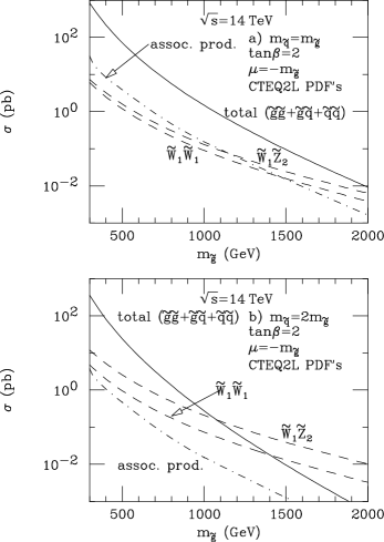
Figure 3: Total SUSY MSSM production cross sections^? at the LHC using $M_{i}=\alpha_{i}M_{\tilde{g}}/\alpha_{s}$ to determine the gaugino masses.

The lowest-order QCD cross sections^?,? for SUSY particle production in the MSSM are shown in Figure 3. These cross sections are similar but not identical to those in the SUGRA model; the gaugino masses are scaled from ${\tilde{g}}$ like

$${M_{1}\over\alpha_{1}}={M_{2}\over\alpha_{2}}={M_{\tilde{g}}\over\alpha_{s}}$$

instead of being calculated from the renormalization group equations. However, the gluino and squark cross sections are model independent, and these dominate except for very high masses and heavy squarks.

In addition to their effects on parton distributions, higher order QCD corrections also give finite ${\cal O}(\alpha_{s})$ corrections to $pp$ cross sections. These corrections typically give significant corrections to the overall normalization. That is, they give

$$\sigma\approx K\sigma_{LO}$$

with a “$K$-factor”

$$K=1+C{\alpha_{s}\over\pi}$$

that is typically substantially larger than one but less than two for the natural lowest-order scale choice because $C\sim\pi^{2}$ rather than $C\sim 1$. While the effect on the normalization is significant, the effect on the shape of inclusive distributions is typically small. This is illustrated in Figure 4, which shows the $p_{T}$ distributions for the leading-order (LO) and next-to-leading-order (NLO) calculations for SUSY production at the LHC.^? The two shapes are clearly almost identical.

Figure 4: Normalized LO and NLO $p_{T}$ distributions^? for squarks and gluinos at the LHC with $M_{\tilde{q}}=600\,{\rm GeV}$, $M_{\tilde{g}}=500\,{\rm GeV}$.

The similarity in the shapes of the LO and NLO distributions seems to be a general feature of perturbative QCD calculations for a wide variety of $pp$ processes. It is partly understood, at least for the simple case of Drell-Yan.^?,? The NLO Drell-Yan calculation contains a $\ln^{2}(-Q^{2})$ factor from the overlapping soft and collinear singularities. The logarithm is canceled by a $\ln^{2}(Q^{2})$ factor for deep inelastic scattering, but there is a $\pi^{2}$ from the difference. This $\pi^{2}$ multiplies the natural scale of $(4\alpha_{s}/3\pi)\sigma_{0}$, where $\sigma_{0}$ is the lowest order cross section, so it produces an overall normalization factor but no change in shape. It is not clear, however, that this $\pi^{2}$ factor is the dominant effect even in the simple case of Drell-Yan.

The cross sections shown in Figure 3 correspond to large rates. “Low” luminosity at the LHC is $10^{33}\,{\rm cm^{-2}s^{-1}}$ (about $10^{2}$ times that currently achieved at the Tevatron) while the design luminosity is $10^{34}\,{\rm cm^{-2}s^{-1}}$. A “Snowmass year” is defined to be $10^{7}\,{\rm s}$, not $3.1536\times 10^{7}\,{\rm s}$; it represents the typical effective running time per year for an accelerator. For example, in the recently completed Tevatron Run I, an integrated luminosity of about $100\,{\rm pb}^{-1}$ was obtained in about two years with peak luminosity of about $10^{31}\,{\rm cm^{-2}s^{-1}}$. Given a luminosity of $10^{4}-10^{5}\,{\rm pb}^{-1}$ per year, a large number of SUSY events will be produced if the masses are below $\sim 1\,{\rm TeV}$, as can be seen from Table 1.

Table 1: Events/year for various SUSY masses at LHC at low and high luminosity using the cross sections shown in Figure 3.

$M_{\tilde{g}}=M_{\tilde{q}}$ (GeV)	$\sigma$ (pb)	Events
500	100	$10^{6}-10^{7}$
1000	1	$10^{4}-10^{5}$
2000	0.01	$10^{2}-10^{3}$

The gluino and squark $p_{T}$ distributions must obviously peak at $p_{T}\sim M$, since smaller $p_{T}$’s are suppressed by phase space, while larger ones are suppressed by the requirement of additional energy for the initial partons. This peaking can be seen in Figure 4 both for the LO and for the NLO calculations. This means that the gluino or squark decay rest frame and the lab frame are similar, and the decay products in the lab frame are spread out over phase space. Gluinos or squarks decay via several steps to the lightest SUSY particle (LSP), taken to be the ${\tilde{\chi}_{1}^{0}}$. Thus a typical event might be:

$$g+g\to{\tilde{g}}+{\tilde{g}}$$

$${\tilde{g}}\to{\tilde{q}}_{L}\bar{q};\quad{\tilde{q}}_{L}\to{\tilde{\chi}}_{2}^{0}q;\quad{\tilde{\chi}}_{2}^{0}\to{\tilde{\chi}_{1}^{0}}\ell^{+}\ell^{-}({\tilde{\chi}_{1}^{0}}q\bar{q})$$

$${\tilde{g}}\to{\tilde{q}}_{R}\bar{q};\quad{\tilde{q}}_{R}\to{\tilde{\chi}_{1}^{0}}q\,.$$

This example event contains five new particles(!). The ${\tilde{\chi}_{1}^{0}}$ has electroweak couplings and must produce virtual sleptons or squarks when interacting with matter, so interacts weakly and escapes from the detector, giving $\hbox to0.0pt{\hbox to7.95831pt{\hfil/\hfil}\hss}E_{T}$. Signatures for such events involve multiple jets, large $\hbox to0.0pt{\hbox to7.95831pt{\hfil/\hfil}\hss}E_{T}$ from the two weakly-interacting ${\tilde{\chi}_{1}^{0}}$’s, possible leptons from decays of gauginos or sleptons in the cascade decay process, and $b$ jets that are either democratically produced or enhanced by smaller third-generation squark masses and large Yukawa couplings.

All of these features provide handles that can be used to separate the SUSY signals from Standard Model backgrounds. As will be discussed in Section 4 below, the LHC detectors can measure the $E_{T}$ of all jets and leptons, so they can determine $\hbox to0.0pt{\hbox to7.95831pt{\hfil/\hfil}\hss}E_{T}$ (with possible problems from cracks and resolution tails). They can identify and measure electrons and muons well; hadronically decaying $\tau$’s can also be identified, although with more background. Finally, $b$ jets can be tagged using vertex detectors to observe displaced vertices.

The single most important experimental signature for SUSY at the LHC is probably missing transverse energy $\hbox to0.0pt{\hbox to7.95831pt{\hfil/\hfil}\hss}E_{T}$. The Standard Model backgrounds for $\hbox to0.0pt{\hbox to7.95831pt{\hfil/\hfil}\hss}E_{T}$ come from all the possible ways to produce high-$p_{T}$ $\nu$’s:

• $W\to\ell\nu$, $\tau\nu$

• $Z\to\nu\bar{\nu}$, $\tau\tau$

• $Q\bar{Q}\to\ell\nu X$, $Q=c,b,t$.

• $g\to Q\bar{Q}$, $Q\to\ell\nu X$

The electroweak cross sections are suppressed by powers of $\alpha$, while the heavy quark ones are suppressed by color and spin factors. Both are suppressed by leptonic branching ratios and by the fact that the missing $\nu$ typically has smaller $p_{T}$ than its parent. There are also backgrounds to $\hbox to0.0pt{\hbox to7.95831pt{\hfil/\hfil}\hss}E_{T}$ from cracks and resolution tails in the detector. These are difficult to estimate in any simple way, but detailed calculations indicate that real neutrinos dominate for events with multiple jets and/or leptons and $\hbox to0.0pt{\hbox to7.95831pt{\hfil/\hfil}\hss}E_{T}\mathrel{\hbox to0.0pt{\raise 2.20013pt\hbox{$>$}\hss}{\lower 2.20013pt\hbox{$\sim$}}}100\,{\rm GeV}$.

3 Event Simulation

SUSY signatures typically involve multiple jets and/or leptons plus missing transverse energy $\hbox to0.0pt{\hbox to7.95831pt{\hfil/\hfil}\hss}E_{T}$ arising from complex cascade decays. The Standard Model backgrounds for these signatures arise only from high orders of perturbation theory, and the dominant contributions come from those regions of phase space that give soft or collinear singularities. Thus it is appropriate to use Monte Carlo event generators that simulate complete events and include the most important effects of QCD radiation to calculate both the signals and the backgrounds. Such event generators also provide complete events that can be used to estimate detector-induced backgrounds.

Three general-purpose event generators are in common use: HERWIG^?, ISAJET^?, and PYTHIA.^? Of these, HERWIG provides the best theoretical treatment of QCD but presently contains no SUSY processes. ISAJET has the most detailed treatment of SUSY. PYTHIA provides a well-tuned description of QCD and hadronization plus many SUSY processes. While a precise description of QCD and hadronization may eventually be important, it it probably not essential for the exploratory studies now being done.

Any Monte Carlo event generator requires a random number generator. If the numbers were truly random, then each run would produce different results, and debugging would be nearly impossible. Hence we require a pseudo-random number generator that produces the same sequence of random numbers given the same initial seed(s). A commonly used algorithm is the congruential generator.^? It is surprisingly simple:

$$s_{0}>0\,,$$

$$s_{n+1}=(as_{n}+c)\mathop{\rm mod}m\,.$$

For careful choices of $a$ and $c$ and a large value of $m$, e.g. $a=7^{5}$, $c=0$, $m=2^{31}-1$ or $a=6909031764870$, $c=0$, $m=2^{48}$, this algorithm yields a uniformly distributed sequence of integers satisfying most tests of randomness. (It is obvious that there are also extremely bad choices.) Then $x_{n}=s_{n}/m$ provides a uniformly distributed real number in $(0,1)$. The congruential generator does have the limitation that $k$-tuples of $x_{n}$ lie on at most $m^{1/k}$ planes in $k$-space. The random number algorithm does not at this time seem to be the critical issue for LHC SUSY physics, so we will not discuss it further here.

3.1 Hard Processes and Perturbative QCD

Given a random number generator, one can construct an algorithm for generating events according to any desired parton processes. This section outlines the basic steps, but since this Summer School is devoted to SUSY rather than to QCD, it opts for simplicity rather than attempting to review the state of the art.^?

Step 1: Generate the parton process. i.e., pick the kinematic variables according to the appropriate lowest order parton cross section. Using a lowest order cross section is important: higher order cross sections would involve singular distributions. These can be treated in principle using a cutoff, but the resulting distributions have very large positive/negative weight fluctuations.

This step is simple in principle, although it may be complicated in practice. From the definitions of cumulative probability distributions and random variables, if $x$ is distributed according to a (normalized) probability distribution $f(x)$, $0<x<1$, then

$$\int_{0}^{x}dx^{\prime}\,f(x^{\prime})=\zeta,\quad 0<\zeta<1\,,$$

where $\zeta$ is a uniformly distributed random variable that can be generated using a congruential or other generator. In a few cases, e.g. $f(x)=(n+1)x^{n}$, this relation can be solved analytically. Generally, an analytic solution is not possible, but one can find a bound $f(x)<f_{\rm max}$ and use a rejection algorithm, accepting $x=\zeta_{1}$ if $f(x)>\zeta_{2}f_{\rm max}$. It is possible to combine these methods and/or change variables to improve the efficiency.

To generate a parton process like $gg\to{\tilde{g}}{\tilde{g}}$, one should choose a set of variables like $p_{T},y_{1},y_{2},\phi$ to isolate the rapid cross section variation in a just a few variables, e.g., $p_{T}$. For processes like gluon and light quark jets that do not involve a mass scale, some form of importance sampling or weighting should be used to generate $p_{T}$ efficiently. For process like $Z$ or $H$ with a narrow $s$-channel resonance, one should instead choose a set of variables such as $\hat{s},\hat{t},\hat{y},\phi$. Generating the hard scattering is basically straightforward, although it can involve rather complex computer code.

Step 2: Add QCD radiation. Perturbation theory describes inclusive cross sections, but it does not necessarily give a good description of event structure. QCD is approximately scale invariant, with a dimensionless coupling $\alpha_{s}$ whose running with $Q^{2}$ is only logarithmic. Hence, radiation at all $Q^{2}$ scales is important; it produces fixed angle jets with $0\ll\langle M^{2}_{\rm jet}\rangle\sim\alpha_{s}(p_{T}^{2})p_{T}^{2}\ll p_{T}^{2}$.

The most important QCD radiation is the emission of gluons collinear with initial or final partons. But we know from the factorization theorems of perturbative QCD that collinear singularities factorize, not for amplitudes but for cross sections. That is,

$$\sigma_{n+1}\sim\sigma_{n}\otimes{\alpha_{s}(p^{2})\over 2\pi p^{2}}P_{ij}(z),\quad p^{2}\to 0\,,$$

where $P_{ij}$ is the appropriate Altarelli-Parisi (DGLAP) function and $z\sim p_{i}/p$. The starting point for QCD-based event generators like HERWIG, ISAJET, and PYTHIA is to use this collinear approximation for gluon radiation together with exact, non-collinear kinematics. This is known as the branching approximation.^? The branching approximation correctly describes the dominant, leading-log QCD effects, but because it uses exact kinematics, it also gives a fairly good approximation for real higher-order QCD effects such as multiple jet production.

The discussion that follows is limited only to the simplest case of leading-log gluon radiation from an outgoing quark line. This does not represent the state of the art, but it is simple to present and illustrates the main point, namely that a classical branching process can provided a reasonable approximation to QCD to all orders in perturbation theory. The cross section for the radiation of $n$ gluons from an outgoing quark is given in the collinear limit by

$$\frac{1}{\sigma}{d\sigma\over dp_{1}^{2}dz_{1}\ldots dp_{n}^{2}dz_{n}}=\left[{\alpha_{s}(p_{1}^{2})\over 2\pi p_{1}^{2}}P(z_{1})\right]\ldots\left[{\alpha_{s}(p_{n}^{2})\over 2\pi p_{n}^{2}}P(z_{n})\right]\,.$$

where $z$ is the momentum fraction. While $z$ is well defined in the collinear limit, its non-collinear extension is model dependent. A good choice is

$$z_{i}={E_{i+1}+|\vec{p}_{i+1}|\over E_{i}+|\vec{p}_{i}|}\,.$$

With this choice, radiation from the quark and antiquark in $e^{+}e^{-}\to q\bar{q}$ is treated symmetrically.

Introduce a minimum mass $t_{c}$ to regulate both the soft and the collinear singularities. For a branching $t_{0}\to t_{1}+t_{2}$ in the initial $t_{0}$ rest frame, the final energy and momenta are given by simple two-body kinematics:

$$E_{1}^{*}={t_{0}+t_{1}-t_{2}\over 2\sqrt{t_{0}}}\,,\qquad p_{1}^{*}={[(t_{0}-t_{1}-t_{2})^{2}-4t_{1}t_{2}]^{1/2}\over 2\sqrt{t_{0}}}\,.$$

The minimum energy and momentum of decay product 1 depend on the relation between the mass and velocity of the decaying system, but the maximum energy and momentum always correspond to $\cos\theta=1$. Boosting the center of mass momenta back to the lab frame, we find

$$z_{\rm max}=1-z_{c}={t_{0}+t_{1}-t_{2}\over 2t_{0}}+{[(t_{0}-t_{1}-t_{2})^{2}-4t_{1}t_{2}]^{1/2}\over 2t_{0}}\,.$$

Setting $t_{1}=t_{2}=t_{c}$, the cutoff mass, gives

$$z_{c}=\frac{1}{2}\left[1-\sqrt{1-{4t_{c}\over t_{0}}}\right]\,.$$

This cutoff will be used in what follows.

The next step is to sum up the radiation softer than the cutoff into a Sudakov form factor, i.e., into the probability of evolving from an initial mass $t$ to a final mass $t^{\prime}$ emitting no resolved radiation greater than the cutoff. The calculation of this Sudakov form factor is particularly simple if one takes the cutoff to be not a fixed mass $t_{c}$ but a fixed smallest $z_{c}$ defined by the initial mass and $t_{c}$ cutoff. Kinematics requires

$$t\geq t_{1}\geq\ldots\geq t^{\prime}\,.$$

By definition of a $z$ cutoff, all the $z_{i}$ are in the interval

$${\cal R}=\{z<z_{c}\}\cup\{z>1-z_{c}\}\,.$$

Thus, using the factorized form for gluon emission, the Sudakov form factor $S$ is given by

$$S_{i}(t,t^{\prime}) =\displaystyle\sum_{n}\int_{t^{\prime}}^{t}dt_{1}\,{\alpha_{s}(t_{1})\over 2\pi t_{1}}\int_{t^{\prime}}^{t_{1}}dt_{2}\,{\alpha_{s}(t_{2})\over 2\pi t_{2}}\ldots\int_{t^{\prime}}^{t_{n-1}}dt_{n}\,{\alpha_{s}(t_{n})\over 2\pi t_{n}}$$

$$\quad\times\displaystyle\int_{\cal R}dz_{1}P_{i}(z_{1})\ldots\int_{\cal R}dz_{1}P_{i}(z_{1})\,.$$

The form of this expression is simple because using a $z$ cutoff decouples the $z$ integrals from the $t$ ones.

Virtual graphs contribute $\delta(1-z)$ terms to the DGLAP functions. Momentum conservation requires that the $x$-weighted integral of the gluon and quark distributions give the total momentum fraction, unity:

$$\int_{0}^{1}dx\,\left[xg(x,Q^{2})+\sum_{q}xq(x,Q^{2})\right]=1\,.$$

This fixes the constants $c_{qq}$ and $c_{gg}$ in the DGLAP functions to satisfy

$$\int_{0}^{1}dz\,\left[{P_{ii}(z)+c_{ii}\delta(1-z)}\right]=0\,,$$

where the $1/(1-z)$ singularities in the functions $P(z)$ are regulated using ”$+$” distributions:

$$\int dz\,{f(z)\over(1-z)_{+}}\equiv\int dz\,{f(z)-f(1)\over(1-z)}\,.$$

The physical meaning of these $+$ distributions is that the soft singularities cancel between the real and virtual graphs. Because the complete integral over $P$ vanishes, the $z$ integrals in the definition of $S$ over the unresolved soft radiation in the region ${\cal R}$ can be related to a well-defined integral over non-soft values of $z$ in the complement of ${\cal R}$:

$$\int_{\cal R}dz\,P_{i}(z)=-\int_{z_{c}}^{1-z_{c}}dz\,P_{i}(z)\equiv-\gamma_{i}(z_{c})\,.$$

The integrals in the definition of $S$ over the $t_{i}$ are elementary, and the nesting gives a factor of $1/n!$. The final result has the simple form

$$S_{i}(t,t^{\prime})=\left[{\alpha_{s}(t)\over\alpha_{s}(t^{\prime})}\right]^{\frac{2}{b_{0}}\gamma_{i}(z_{c})}\,.$$

Knowing the cumulative distribution $S$ is enough to generate the next mass and hence the complete shower. Given $S$, the probability $\Xi(t)$ that the first resolved radiation occurs at $t$ is given by

$$\int_{t_{c}}^{t_{0}}dt\,\Xi(t)=1-S_{i}(t_{0},t_{c})\,.$$

The mass-squared $t$ of the quark at the next branching is therefore generated by solving the equation

$${1-S_{i}(t,t_{c})\over 1-S_{i}(t_{0},t_{c})}=\zeta\,,$$

where $\zeta$ is a uniformly distributed random number in $(0,1)$. Given the form for $S$, this equation can be easily solved in terms of elementary functions. This solution can then be used to build the complete shower:

1. Generate $t$.

2. Generate $z_{c}<z<1-z_{c}$ according to $P_{i}$.

3. Check $z$ against $t_{c}$ limits.

4. Generate $t_{1}$, $t_{2}$ starting at $z$, $(1-z)t$.

5. Solve 2-body kinematics.

6. Iterate.

This simple Monte Carlo algorithm generates all the leading-log effects of QCD radiation and provides a reasonable approximation to non-leading effects such as multi-jet production.

The algorithm just described can be extended to include $g\to gg,q\bar{q}$ and initial state radiation. It can also be refined in various ways, in particular to include in an approximate way coherent interference effects that reduce the radiation of soft gluons. For a recent review see Webber.^?

Step 3: Generate decays of the SUSY particles. This involves selecting the decay mode using branching ratios calculated from the SUSY masses and couplings and then then generating the decay using 2-body or 3-body phase space. Parton showers from any outgoing quarks or gluons are added using the branching approximation with an initial scale equal to the parent particle mass.

The use of phase space for a 3-body decay, say ${\tilde{q}}\to{\tilde{\chi}_{1}^{0}}q\bar{q}$, is not a good approximation if the squark ${\tilde{q}}$ is just slightly heavier than the gluino. The squark poles should cause the matrix element to peak where the gaugino and one quark are hard, while the other quark is soft. All distributions should be continuous as the squark mass varies from below to above the gluino mass, but the phase space approximation is not. This problem does not affect any of the points to be studied here. The approximations also lose information on spin correlations between particles, but this is probably not very important, at least for LHC studies.

Step 4: Hadronize the partons, i.e., generate a jet of hadrons for each parton. This involves soft, nonperturbative QCD physics, so one must rely on models tuned to experimental fragmentation data. The physical picture is that the hard scattering creates separated color charges connected by “strings” of gluons. As the strings stretch, they break, pulling a $q\bar{q}$ pair out of the vacuum. Since QCD is strong only at low $Q^{2}$, this breaking is a soft process which only occurs with low $p_{T}$ and small $\Delta y$. Thus it produces a jet of hadrons with limited $p_{T}$ relative to the parton direction. Hence, the event structure is mainly controlled by perturbation theory, not by the soft physics model.

The hard part of a $pp$ interaction never accounts for more than a small fraction of the total energy. The rest of the energy is carried off by spectators, which produce low-$p_{T}$ hadrons more or less uniformly in rapidity. Typically the leading particle in the beam jet carries half of the beam energy and just a few hundred MeV of transverse momentum. As a result, much of the energy escapes down the beam pipe: one can measure missing transverse energy $\hbox to0.0pt{\hbox to7.95831pt{\hfil/\hfil}\hss}E_{T}$ but not missing total energy. The models for beam jets are essentially parameterizations of experimental data. Fortunately, the beam jets are not very important for the experimental signatures, although they do have some effect on the isolation requirements for leptons and photons.

3.2 Soft or $\ln s$ Physics

The production of SUSY particles and of all the significant Standard Model backgrounds for them are hard processes that can be calculated in QCD perturbation theory. But most of the events at the LHC are soft interactions, for which there is no good theoretical description. These events are not important as backgrounds for new physics, but they dominate the rate and so are important for the design of the detectors. Fortunately, soft physics varies slowly with $\ln s$, so reliable extrapolations from lower energy can be made even without a good theoretical model.

The geometrical size of the proton is set by $1/M_{\pi}$, implying a natural geometrical cross section

$$\sigma=\pi\left({\hbar c\over M_{\pi}}\right)^{2}\approx 62\,{\rm mb}$$

since $\hbar c=197\,\hbox{MeV-f}$. This should be compared with SUSY cross sections ranging from $0.01\,{\rm pb}$ to $100\,{\rm pb}$ depending on the masses. The total cross section is of course given by the imaginary part of the forward scattering amplitude,

$$\sigma_{T}={1\over s}\Im f(s,0)\,.$$

In the high energy limit with fixed momentum transfer ($s\to\infty$, $t$ fixed) the exchange of an elementary particle of spin $J$ in the $t$ channel leads to

$$f(s,t)\sim P_{J}(z_{t})\sim s^{J}\,.$$

The Froissart bound, based only on analyticity properties that can be proven in field theory and on unitarity of the $S$-matrix, limits the growth of the cross section to

$$\sigma_{T}\leq\hbox{const}\ln^{2}s$$

so we must have $J\leq 1$.

The experimental data on the $pp$ and $\bar{p}p$ total cross sections, Figure 5, show rapid variation at low energy and large differences between the $pp$ and $\bar{p}p$. This difference is not surprising, since $\bar{p}p$ has a large cross section to annihilate into mesons, while $pp$ cannot do this. At high energy, however, the $pp$ and $\bar{p}p$ cross sections become equal and vary slowly with $\ln s$, in a way quite consistent with the Froissart bound.

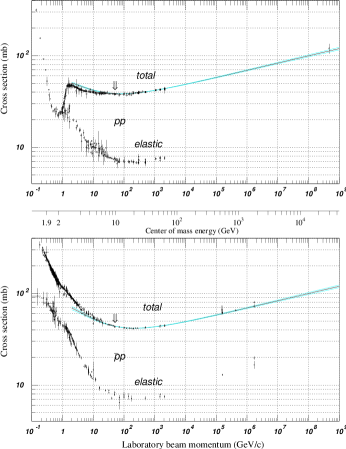
Figure 5: Compilation of $pp$ and $\bar{p}p$ cross sections.^?

While the total cross section is certainly nonperturbative, it is useful to consider how multiparticle production works in perturbation theory. Because the gluon has spin one, the box graph, Figure 6, gives a constant cross section for large $s$. Of course the cross section is infinite for a massless gluon exchanged between unconfined quarks, so an infrared cutoff is needed. Hence this whole discussion is only qualitative. However, it is possible to do a rigorous calculation of the behavior of the high-$p_{T}$ jet cross section for $s\gg p_{T}^{2}$ in QCD perturbation theory.^?

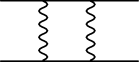
Figure 6: The discontinuity of the box graph gives a constant cross section for $s\to\infty$.

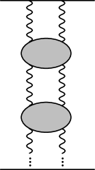
Figure 7: The discontinuity of the (generalized) ladder graph gives a factor of $\ln s$ from each longitudinal phase space integral.

The generalized ladder graph in Figure 7 similarly remains constant as the generalized rungs, the shaded blobs in the figure, are moved in rapidity. Hence, this graph gives a factor of $\ln s$ from each longitudinal phase space integral. It can be shown that graphs like this give the leading powers of $\ln s$ for each order in perturbation theory. The $n$ longitudinal integrals are ordered in rapidity and so give

$$\int_{0}^{\ln s}dy_{1}\dots\int_{0}^{y_{n-1}}dy_{n}={1\over n!}\ln^{n}s\,.$$

The discontinuity across the generalized rungs produces particles in the final state, and the distribution of these particles, like that of the rungs, is flat in rapidity. Furthermore, after many steps in rapidity, any quantum number exchange will be washed out, so the distribution in the central region is universal. All of these properties of this toy model are in qualitative agreement with experiment. However, the growth of Figure 7 with $\ln s$ violates the Froissart bound, so more complicated graphs must become important.

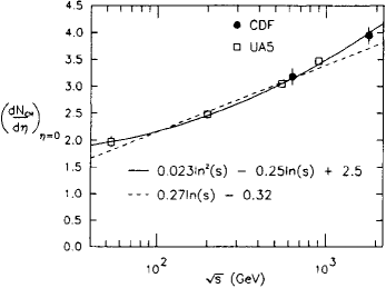
Figure 8: Compilation of $dN/d\eta\approx dN/dy$ for $pp$ and $\bar{p}p$ interactions.^?

Data on the charged multiplicity $dN/d\eta$, where

$$\eta\equiv-\ln\tan{\theta\over 2}\approx y\equiv\ln{E+p_{L}\over E-p_{L}}\quad{\rm for}\quad p_{T}\gg m\,,$$

are shown in Figure 8 for $pp$ and $\bar{p}p$ interactions. The rise is consistent with either a power of $\ln s$ or a small power of $s$. A smooth extrapolation to $14\,{\rm TeV}$ gives

$${dN_{\rm ch}\over d\eta}\approx 6\,.$$

The mean $p_{T}$ also grows slowly with $\sqrt{s}$, rising from about $0.35\,{\rm GeV}$ at low energy to about $0.5\,{\rm GeV}$ at $1.8\,{\rm TeV}$. Most of this rise probably comes from QCD jets with transverse momenta of a few GeV. Extrapolation suggests $\langle p_{T}\rangle\sim 0.65\,{\rm GeV}$ at LHC.

Soft interactions do not produce backgrounds for SUSY or other interesting processes, but they do give a very high interaction rate. The LHC bunch crossing rate is $40\,{\rm MHz}$, and there are $\sim 2$ interactions/bunch at $10^{33}\,{\rm cm^{-2}s^{-1}}$ and $\sim 20$ interactions/bunch at $10^{34}\,{\rm cm^{-2}s^{-1}}$.

4 LHC Detectors

Two LHC large detectors, ATLAS^? and CMS,^? are just beginning construction. Both ATLAS and CMS are designed to identify and measure all the Standard Model quanta — $\gamma$, $e$, $\mu$, $\tau$, $g$ and $q$ jets, and $b$ jets — over $|\eta|\mathrel{\hbox to0.0pt{\raise 2.20013pt\hbox{$<$}\hss}{\lower 2.20013pt\hbox{$\sim$}}}2.5$ ($\theta\mathrel{\hbox to0.0pt{\raise 2.20013pt\hbox{$>$}\hss}{\lower 2.20013pt\hbox{$\sim$}}}10^{\circ}$) and to measure energy flow over $|\eta|\mathrel{\hbox to0.0pt{\raise 2.20013pt\hbox{$<$}\hss}{\lower 2.20013pt\hbox{$\sim$}}}5$ ($\theta\mathrel{\hbox to0.0pt{\raise 2.20013pt\hbox{$>$}\hss}{\lower 2.20013pt\hbox{$\sim$}}}1^{\circ}$) to determine the missing transverse energy $\hbox to0.0pt{\hbox to7.95831pt{\hfil/\hfil}\hss}E_{T}$. This broad coverage is essential for complex signatures like SUSY. The cost of each detector by CERN accounting rules is CHF 475M. Each collaboration currently includes about 1500 physicists and senior engineers. Thus, both ATLAS and CMS are more like laboratories than traditional experiments.

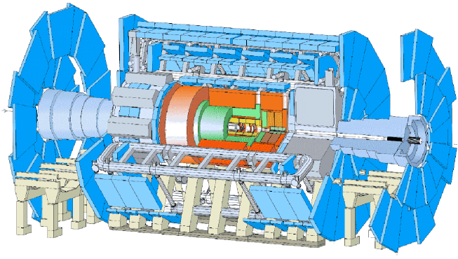
Figure 9: Cutaway view of the ATLAS detector^? as of 1997, showing from inside out the central detector, 2 Tesla solenoidal magnet coil, liquid argon electromagnetic calorimeter, hadron calorimeter and muon system including the lumped toroidal magnet coils and three layers of muon chambers.

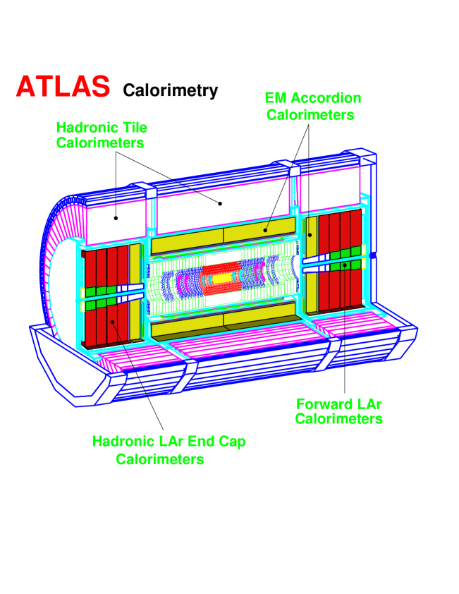
Figure 10: Cutaway view of the ATLAS calorimeter and central tracker, the central part of Figure 9.

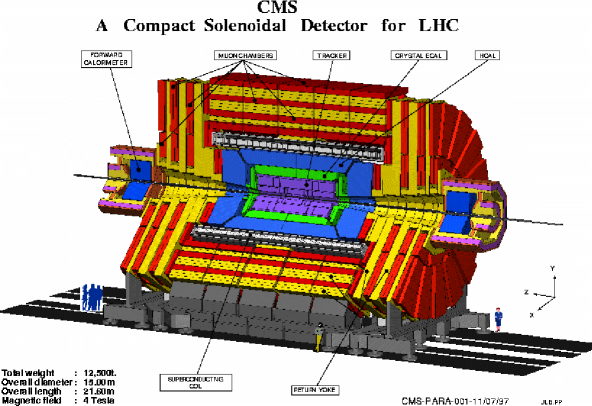
Figure 11: Cutaway view of the CMS detector^? as of 1997, showing from inside out the central tracker, crystal electromagnetic calorimeter, hadron calorimeter, 4 Tesla solenoidal magnet coil, and muon system.

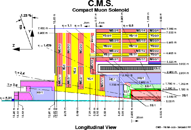
Figure 12: Cross section of one quarter of the CMS detector,^? showing the same elements as Figure 11.

The cost and scale of the detectors is driven both by the need to measure the high energies and large range of possible interesting processes such as SUSY production and by the need to cope with the high rates caused by soft physics at the LHC. While the detectors are quite different in detail, they both have the same basic elements. These are from inside out: a silicon vertex detector intended primarily for tagging $b$ jets, an inner tracker to measure the momenta of charged particles in a magnetic field, an electromagnetic calorimeter to measure the energies and directions of photons and electrons, a hadron calorimeter to measure jets, a forward calorimeter mainly to measure $\hbox to0.0pt{\hbox to7.95831pt{\hfil/\hfil}\hss}E_{T}$ but also to tag forward jets, and a muon system to identify and to measure muons. These parts can be seen in Figures 9 – 12. Section 4.1 below gives a brief description of each of these elements and their most important performance parameters. This is followed by Section 4.2, which explains how the parts are used in combination to detect physics signatures. The discussion given here is necessarily superficial, but hopefully it will prove useful to theorists interested in LHC physics. For details the reader should see the ATLAS^? and CMS^? Technical Proposals and the Technical Design Reports for the detector subsystems. The Particle Data Group^? provides useful general information on particle detectors.

4.1 Detector Elements

Silicon vertex detector: Both ATLAS and CMS have silicon microstrip detectors covering $|\eta|<2.5$. These are primarily intended to tag $b$ jets by detecting the displaced vertices of $B$ hadrons, but they also contribute to the momentum measurement. The detector elements are made out of silicon wafers similar to those used to make computer chips. A charged particle passing through the silicon causes ionization, and the resulting electrons are collected on strips about $80\,\mu{\rm m}$ wide. An amplifier and discriminator on each strip determines which strips were hit. For a uniform distribution of a variable $x$ in an interval $(-a/2,a/2)$,

$$\langle x^{2}\rangle={1\over a}\int_{-a/2}^{a/2}dx\,x^{2}={a^{2}\over 12}\,,$$

so the nominal resolution orthogonal to the strip direction is about $80\,\mu{\rm m}/\sqrt{12}$. The resolution in practice is very similar. Measurement of the other coordinate is obtained by using small-angle stereo, i.e., by placing the strips of adjacent layers at a small angle. The innermost layers of the silicon detectors will use pixels of about $50\,\mu{\rm m}\times 300\,\mu{\rm m}$ rather than strips. These are still under development.

Central Tracker: Given the high multiplicity at the LHC, it is a difficult problem in pattern recognition to combine the right hits to find the real tracks. Having many layers in the tracking system helps, but it is prohibitive in terms of both cost and material to make many silicon layers. In ATLAS the outer portion of the tracker uses 70 layers of straw tubes. These have a thin conducting outer shell and a fine wire in the center, with a high voltage between them. Charged particles produce ionization in the gas, which is chosen to give a constant drift velocity for the produced electrons. These electrons drift to the central wire, where the high field produces an avalanche with a typical gas gain of $\sim 10^{4}$. The time of this signal is measured, and the drift velocity is used to convert this to a drift distance with a resolution of order $100\,\mu{\rm m}$.

The ATLAS tracker is a “Transition Radiation Tracker.” It also incorporates a transition radiation detector, which detects the $X$-rays emitted by a charged particle passing through a dielectric interface. This radiation is proportional to $\gamma$ and is useful for identifying low-$p_{T}$ electrons.

The CMS outer tracker uses gas microstrip detectors, which are still being developed. The ionization is produced in a layer of gas, but it is detected using closely spaced strips on a substrate read out in a manner similar to silicon strips. There are fewer layers than in the ATLAS tracker, but each layer has better position resolution and lower occupancy.

The purpose of the central tracker is to determine the momenta of charged particles by measuring their curvature in the central solenoidal magnetic field. As a consequence of the Lorentz force, $F=e\vec{v}\times\vec{B}$, a charged particle in a uniform solenoidal magnetic field $B$ follows a helix with a radius of curvature

$$R={p_{T}\over 0.3B}\,,$$

with $R$ in meters, $B$ in Tesla, and $p_{T}$ in GeV. Simple geometry shows that the resulting sagitta $s$ for a radial length $L\ll R$ is given by

$$s={L^{2}\over 8R}={0.3BL^{2}\over 8p_{T}}$$

with $s$ and $L$ in meters and $p_{T}$ in GeV. For $p_{T}=100\,{\rm GeV}$, $B=2\,{\rm T}$, and $L=1\,{\rm m}$, the sagitta is $s=750\,\mu{\rm m}$. The resolution depends on the chamber layout and position resolution and on the multiple scattering in the chamber material. ATLAS has $B=2\,{\rm T}$, typical for most detectors, and $R=1\,{\rm m}$, giving

$${\Delta p_{T}\over p_{T}}\approx 0.7\left({p_{T}\over 1\,{\rm TeV}}\right)\oplus 0.014\,,$$

where the constant term comes from multiple scattering and is added in quadrature. The resolution for tracks beyond the corner of the solenoid degrades like $1/\sin^{2}\theta$. CMS has a very high field, $B=4\,{\rm T}$, and also a larger radius, giving

$${\Delta p_{T}\over p_{T}}\sim 0.1\left({p_{T}\over 1\,{\rm TeV}}\right)\,,$$

again degrading beyond the corner of the solenoid. ATLAS has a comparable resolution for muons only using its muon system.

Electromagnetic Calorimeter: Precision electromagnetic calorimetry has been used in several $e^{+}e^{-}$ detectors, but ATLAS and CMS are the first hadron-collider detectors to have it. The demand for very high resolution is driven by the search for $h\to\gamma\gamma$; it will be seen in Section 9 that this gives a narrow peak on a large $\gamma\gamma$ continuum background. The ability to separate $e$ and $\gamma$ depends on the tracker, so the useful calorimeter coverage is also $|\eta|<2.5$.

Any calorimeter creates a shower in some dense material and uses the total charge or light output from this shower to determine the energy of the initiating particle. The energy is divided among more and more particles until it is completely absorbed. It is important to realize that electromagnetic interactions with a dense material like lead are much stronger than hadronic ones: electromagnetic interactions scale like $Z^{2}$ while hadronic ones scale like $A^{2/3}$. For lead, the radiation length $X_{0}$, the distance in which a high energy electron loses all but $1/e$ of its energy, is $0.56\,{\rm cm}$, while the inelastic hadronic interaction length $\lambda$ is $17.1\,{\rm cm}$. (For a light material like aluminum $X_{0}=8.9\,{\rm cm}$ and $\lambda=39.4\,{\rm cm}$.) Thus, an electromagnetic calorimeter $\sim 25X_{0}$ thick will contain almost all of the shower from high energy electrons or photons while absorbing little hadronic energy. Thus the electromagnetic calorimeter is always in front of the hadronic one.

The ATLAS electromagnetic calorimeter uses lead plates with gaps filled with liquid argon. Electrons from the shower drift under high voltage through the liquid argon and are collected on readout pads. The energy is proportional to the total charge, with an energy resolution

$${\Delta E\over E}\approx{10\%\over\sqrt{E}}\oplus 0.5\%$$

with $E$ measured in GeV. The first term here comes from the shower multiplicity and the fluctuations in sampling it: the multiplicity $N$ of particles in the shower is proportional to the energy, and the Poisson fluctuation in $N$ is $1/\sqrt{N}$. Note that this term gives the same resolution for one particle or from several with the same total energy, the errors being added in quadrature, as one would expect for a calorimeter. The small constant term arises from many sources and is added in quadrature. The ATLAS calorimeter can also use the position of the shower as a function of depth to measure the direction of a photon with an accuracy of about $50\,{\rm mr}/\sqrt{E}$.

CMS uses a dense, transparent crystal, ${\rm PbWO_{4}}$, both to create the shower and to convert it into scintillation light that can be detected by photodiodes. Because there are no inert lead plates, the whole shower can be measured, the sampling fluctuations are reduced, and the resolution is therefore better,

$${\Delta E\over E}\approx{2\%\over\sqrt{E}}\oplus 0.5\%\,,$$

with $E$ measured in GeV. While crystals give better energy resolution, they make it harder to achieve fine segmentation and good pointing accuracy, and controlling the crystal quality is not trivial. At low luminosity, CMS will rely on tracking to determine the vertex and hence the photon direction. At high luminosity, it will add a preshower detector to measure the starting position of the shower and provide directional information at the cost of some energy resolution.

Hadron Calorimeter: The hadron calorimeter follows the electromagnetic one and measures the energy of both charged and neutral hadrons. Hadronic showers have intrinsically larger fluctuations than electromagnetic ones, and additional errors are introduced for jets by the clustering algorithm. Both the ATLAS and the CMS central hadron calorimeters use steel plates (which also act as the magnetic flux return) and sample the hadronic showers with scintillators read out by photomultiplier tubes. (The ATLAS endcap hadron calorimeter uses copper plates and liquid argon.) The resulting jet resolutions when combined with the electromagnetic calorimeters are roughly

$${\Delta E\over E}\approx{60\%\over\sqrt{E}}\oplus 3\%\,,\qquad|\eta|<3\,,$$

with $E$ measured in GeV. The first term comes from the shower multiplicity and the fluctuations in sampling it, as for the electromagnetic calorimeter. The second term is added in quadrature and comes, e.g., from the fact that there are fluctuations in the fraction of the energy carried by $\pi^{0}$’s and by charged $\pi$’s, and the calorimeter responds differently to these. The forward calorimeters cover $3<|\eta|<5$ with cruder energy resolution since $E\gg p_{T}$ in this region.

Solenoid: The central trackers require solenoids to provide the magnetic field. The 2 Tesla solenoid in ATLAS is thin, $<1X_{0}$, so it can be placed in front of the electromagnetic calorimeter without degrading its resolution too much. The 4 Tesla solenoid in CMS must be much thicker and so must be placed outside the hadron calorimeter.

Muon System: Muons radiate much less than electrons and so penetrate the whole calorimeter with small energy losses, at least for energies below the TeV scale. ATLAS makes its precise muon measurement with an air-core toroidal magnet outside the calorimeter and three groups of tracking chambers to measure the resulting sagitta. The barrel toroid is made of eight lumped coils, which can be seen in Figure 9. Lumped coils are needed to allow chambers to be placed within the toroid but give a rather complex, non-uniform field. The endcap toroid has one group of chambers in front of it and two groups behind it. The resolution $p_{T}$ for large $p_{T}$ in the central region is

$${\Delta p_{T}\over p_{T}}\sim 10\%\left({p_{T}\over 1\,{\rm TeV}}\right)\,;$$

it remains quite good up to $\eta=2.5$ because the endcap toroid gives a $B\propto 1/r$ at small radius, thus increasing the bending power at large $\eta$.

Table 2: A set of possible Level 1 and Level 2 triggers for ATLAS^? at ${\cal L}=10^{34}\,{\rm cm^{-2}s^{-1}}$. The $\hbox to0.0pt{\hbox to7.95831pt{\hfil/\hfil}\hss}E_{T}$ thresholds are not yet known but should be $\sim 100\,{\rm GeV}$; they will be set to give the indicated rates.

Trigger Requirement	LVL1 Rate	LVL2 Rate
	(kHz)	(kHz)
$\geq 1$ muon, $p_{T}>20\,{\rm GeV}$	4
$\geq 1$ isolated $\mu$, $p_{T}>20\,{\rm GeV}$		0.2
$\geq 1$ $\mu$, $p_{T}>40\,{\rm GeV}$		0.1
$\geq 1$ isolated e.m. cluster, $E_{T}>30\,{\rm GeV}$	20
$\geq 1$ electron $E_{T}>30\,{\rm GeV}$		0.3
$\geq 1$ isol. e.m. cluster, $E_{T}>30\,{\rm GeV}$		0.1
$\geq 2$ muons, $p_{T}>6\,{\rm GeV}$	1
$\geq 2$ $\mu$, $p_{T}>10\,{\rm GeV}$		0.1
$\geq 2$ isolated $\mu$, $p_{T}>6\,{\rm GeV}$		0.01
$\geq 2$ isolated e.m. clusters, $E_{T}>20\,{\rm GeV}$	4
$\geq 2$ $e$ or $\gamma$, $p_{T}>20\,{\rm GeV}$		0.2
$\geq 1$ jet, $E_{T}>150\,{\rm GeV}$	3
$\geq 1$ jet, $E_{T}>300\,{\rm GeV}$		0.1
$\geq 3$ jets, $E_{T}>150\,{\rm GeV}$		0.04
Missing energy ($\hbox to0.0pt{\hbox to7.95831pt{\hfil/\hfil}\hss}E_{T}$)	1	0.1
Prescaled triggers	5	0.1
Total	38	1.4

CMS relies on its central tracking to achieve comparable resolution for both muons and hadrons, making only a $\sim 20\%$ measurement in the external muon system, which utilizes the iron flux return of the central solenoid for its magnetic field. The CMS muon system provides triggering and muon identification rather than a precise measurement.

Trigger: The trigger systems are crucial for the LHC experiments. The $40\,{\rm MHz}$ interaction rate must be reduced by about a factor of $10^{6}$ before the events can be saved to tape for future analysis, and this obviously limits the physics that can be studied. The trigger is divided into three levels. Level 1 is hardware-based, synchronous with the beam clock, and deadtimeless. The data from every detector element must be saved for about $2\,{\rm\mu s}$ until a Level 1 decision can be made. This decision is based on fast sums of predefined clusters in the electromagnetic and hadronic calorimeter and on hits in roads corresponding to stiff tracks in the muon system. The thresholds on these are adjusted to reduce the rate to about $10^{4}\,{\rm Hz}$. Level 2 refines the selection made at Level 1 by using the full granularity of the detector and by combining measurements from more than one subsystem in “regions of interest” found by Level 1 trigger. This allows one, e.g., to determine the $p_{T}$ of an electron candidate more accurately both by using more detailed calorimeter information and by comparing it with tracking information. Finally, at Level 3 the whole detector is read out into a computer farm, which can run off-line analysis code and save events at roughly $100\,{\rm Hz}$. A list of possible triggers for ATLAS and their Level-1 and Level-2 rates is shown in Table 2.

4.2 Measuring the Standard Model Quanta

Any SUSY or other new particle will be produced at the LHC with $p_{T}\mathrel{\hbox to0.0pt{\raise 2.20013pt\hbox{$<$}\hss}{\lower 2.20013pt\hbox{$\sim$}}}M$, so its decay products will be widely distributed in phase space. It will either decay into quanta of the Standard Model — quark or gluon jets, charged leptons, neutrinos, or photons — or it will be stable and escape the detector like the lightest SUSY particle ${\tilde{\chi}_{1}^{0}}$ if $R$ parity is conserved. ATLAS and CMS are designed to detect such signals, in many cases with redundant measurements.

Jets: Jets, the dominant signal at large $p_{T}$, are measured as clusters of energy in the electromagnetic and hadronic calorimeters. There will also be multiple charged tracks connecting this cluster and the vertex. The jet energy resolution tends to be dominated more by uncertainties associated with jet clustering and QCD radiation than by detector performance.

$b$ Jets: The most important use of the vertex detector is to tag $b$ jets. Most of the tracks in an event will point back to the primary vertex, but those from a $B$ hadron will have a distance of closest approach characteristic of the $B$ lifetime, i.e., $c\tau\approx 465\mu{\rm m}$. Tagging is not easier for a highly relativistic $B$ hadron: while the typical distance traveled by the $B$ is $\gamma c\tau$, the typical opening angles of the decay tracks are ${\cal O}(1/\gamma)$, so the typical distance of closest approach to the primary vertex is independent of $\gamma$ provided $\beta\approx 1$. Calculating the tagging efficiency requires detailed simulation and obviously involves a tradeoff between efficiency and background rejection. For a 1% mistagging rate for light quark jets, the typical tagging efficiency is 60%.^?

Photons: An isolated photon is identified as a cluster contained in the electromagnetic calorimeter with a radius of order the radiation length $X_{0}$ with no hadronic energy behind it and no high-$p_{T}$ charged track near it. (Actually, the trackers in ATLAS and CMS both contain a significant fraction of $1X_{0}$, so the probability that the photon converts to an $e^{+}e^{-}$ pair in the tracker is not small.) Isolation criteria are sufficient to reject jets by a factor of several thousand but still leave some background from those jets in which one or more $\pi^{0}$’s carry most of the jet energy. An additional rejection can be obtained by using a preradiator to count the number of photons and/or by using detailed shower shape cuts. Thus, because of the very good ATLAS and CMS electromagnetic calorimeters, a jet rejection of $\sim 10^{4}$ can be achieved with a photon efficiency of order 90%. Hence, the background for $h\to\gamma\gamma$ should be dominated by the real QCD $\gamma\gamma$ continuum. Non-isolated photons of course cannot be separated from the much larger rate for $\pi^{0}\to\gamma\gamma$ in jets.

Electrons: An electron gives an electromagnetic shower like a photon but has a track with $p\approx E$ pointing to it. Because of this extra constraint, isolated electrons with $p_{T}\mathrel{\hbox to0.0pt{\raise 2.20013pt\hbox{$>$}\hss}{\lower 2.20013pt\hbox{$\sim$}}}10\,{\rm GeV}$ and $|\eta|<2.5$ can be identified with an efficiency of order 90% with a jet rejection of $\sim 10^{5}$, so that the background for isolated electrons is dominated in almost all cases by real electrons. Electrons within jets are much more difficult to identify.

Taus: A $\tau$ decaying into a lepton is difficult to distinguish from a prompt lepton. A $\tau$ decaying into hadrons can be identified as a narrow hadronic jet with one charged track or three tracks with a charge $\pm 1$ and a mass $<M_{\tau}$. The background from QCD jets is significant, and detailed study is required to develop cuts appropriate for any particular case.

Muons: A muon is identified by a charged track in the central tracker and a matching charged track in the external muon system. The energy deposition in the calorimeter is small ($\sim 2\,{\rm GeV}$) for energies below about $1\,{\rm TeV}$. At higher energies bremsstrahlung and $e^{+}e^{-}$ pair production become significant, and the energy deposited in the calorimeter needs to be considered.

Missing Energy: In hadron colliders the total missing energy is completely dominated by the loss of low-$p_{T}$ particles in the beam pipe, so only the missing transverse energy $\hbox to0.0pt{\hbox to7.95831pt{\hfil/\hfil}\hss}E_{T}$ can be used to detect neutrinos or ${\tilde{\chi}_{1}^{0}}$’s. This is measured by summing all the calorimeters plus any observed muons. The resolution is dominated by non-Gaussian tails and cracks in the calorimeter; detailed studies indicate that real neutrinos dominate over the instrumental background at least for $\hbox to0.0pt{\hbox to7.95831pt{\hfil/\hfil}\hss}E_{T}>100\,{\rm GeV}$.

5 Inclusive SUSY Measurements at LHC

If SUSY is indeed the right new physics at the electroweak scale, the first task of the LHC will be to detect a deviation from Standard Model predictions characteristic of SUSY. The ability to do so is clearly model dependent. For example, if all SUSY particles were nearly degenerate in mass, then they would decay into very soft jets or leptons plus an invisible ${\tilde{\chi}_{1}^{0}}$, and nothing would be observable. Fortunately, such a degenerate spectrum does not occur in any reasonable model.

5.1 Simulation of SUSY Signatures

Most recent studies of SUSY signatures at the LHC have assumed the minimal supergravity (SUGRA) model.^? The SUGRA model is a special case of the Minimal Supersymmetric Standard Model (MSSM), with two Higgs doublets and a SUSY partner for each Standard Model one, grand unification at some scale $M_{\rm GUT}$, and soft SUSY breaking terms added by hand assuming $R$-parity conservation:

$$-{\cal L}_{\rm soft} = A^{u}h^{u}\widetilde{Q}H_{u}\widetilde{u}^{c}+A^{d}h^{d}\widetilde{Q}H_{d}\widetilde{d}^{c}+A^{\ell}h^{\ell}\widetilde{L}H_{d}\widetilde{\ell}^{c}$$

$$+B\mu(H_{d}H_{u}+h.c.)+M_{H_{d}}^{2}|H_{d}|^{2}$$

$$+M_{H_{u}}^{2}|H_{u}|^{2}+M_{\widetilde{L}}^{2}|\widetilde{L}|^{2}+M_{\widetilde{e}}^{2}|\widetilde{e}^{c}|^{2}$$

$$+M_{\widetilde{Q}}^{2}|\widetilde{Q}|^{2}+M_{\widetilde{u}}^{2}|\widetilde{u}^{c}|^{2}+M_{\widetilde{d}}^{2}|\widetilde{d}^{c}|^{2}$$

$$+\frac{1}{2}M_{1}\overline{\widetilde{B}}\widetilde{B}+\frac{1}{2}M_{2}\overline{\widetilde{W}}\widetilde{W}+\frac{1}{2}M_{3}\overline{\widetilde{g}}\,\widetilde{g}\,.$$

In SUGRA the soft breaking terms are assumed to be communicated from the SUSY breaking sector by gravity and so to be universal at $M_{\rm GUT}$. The resulting minimal set of parameters is:

• $m_{0}$: the common SUSY-breaking mass of all squarks, sleptons, and Higgs bosons.

• $m_{1/2}$: the common SUSY-breaking mass of all gauginos.

• $A_{0}$: the common SUSY-breaking trilinear coupling.

• $B\mu$: the SUSY-breaking bilinear coupling.

• $\mu$: the SUSY-conserving Higgsino mass.

All of these parameters, including the SUSY-conserving parameter $\mu$, should be of order the weak scale. A limitation of the SUGRA model is the absence of any understanding of why $\mu$ should be of order the weak scale or why $R$ parity should be conserved. For a more detailed discussion, see the lectures by Dawson^? in these Proceedings and references therein.

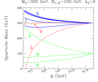
Figure 13: Evolution of SUSY masses from the GUT to the electroweak scale.^?

The SUGRA model defines the SUSY breaking parameters at the GUT scale. All of these parameters are essentially couplings and so obey renormalization group equations (RGE’s). The RGE’s in the SUGRA model involve 26 coupled partial differential equations, which have been studied by various authors;^? an example is shown in Figure 13. ISAJET implements a self-consistent solution of these RGE’s between the weak and the GUT scale. The first step is to run a truncated set of six equations from $M_{Z}$ to the GUT scale where the gauge couplings $g_{1}$ and $g_{2}$ meet using approximate SUSY mass scale:

$${dg_{1}\over dt} =-{1\over 16\pi^{2}}(-\frac{3}{5}-N_{f})g_{1}^{3}+\hbox{2-loop terms}$$

$${dg_{2}\over dt} =-{1\over 16\pi^{2}}(5-N_{f})g_{2}^{3}+\hbox{2-loop terms}$$

$${dg_{3}\over dt} =-{1\over 16\pi^{2}}(9-N_{f})g_{3}^{3}+\hbox{2-loop terms}$$

$$\dots$$

$${dy_{t}\over dt} ={1\over 16\pi^{2}}y_{t}[6y_{t}^{2}-\frac{13}{15}g_{1}^{2}-3g_{2}^{2}-\frac{16}{3}g_{3}^{2}]\,.$$

Once $M_{\rm GUT}$ is determined, the universal SUGRA boundary conditions are imposed, and the full set of 26 RGE’s are run back to the weak scale using Runge-Kutta step-by-step integration so that mass thresholds can be properly taken into account. The Clebsch-Gordon coefficients in these equations are such that the Higgs mass is driven negative, breaking electroweak symmetry but not charge or color. The Higgs effective potential is determined, and the GUT scale parameters $B$ and $\mu^{2}$ are determined in terms of the weak scale parameters $M_{Z}$ and $\tan\beta=v_{2}/v_{1}$. The whole procedure is then iterated until a self-consistent solution is obtained. The final result is to express the masses of all 32 SUSY particles plus all the mixing parameters in terms of just four parameters plus $\mathop{\rm sgn}\mu=\pm 1$:

• $m_{0}$: common scalar mass at $M_{\rm GUT}$.

• $m_{1/2}$: common gaugino mass at $M_{\rm GUT}$.

• $A_{0}$: common trilinear coupling at $M_{\rm GUT}$.

• $\tan\beta=v_{2}/v_{1}$: Ratio of VEV’s at $M_{Z}$.

• $\mathop{\rm sgn}\mu=\pm 1$.

In the SUGRA model the SUSY masses are mainly determined by $m_{0}$ and $m_{1/2}$, while $\tan\beta$ and $\mathop{\rm sgn}\mu=\pm 1$ mainly affect the Higgs sector. $A_{0}$ is not very important for weak-scale physics; while $A_{t}$, $A_{b}$, and $A_{\tau}$ are important for third-generation sparticles, they turn out to be only weakly dependent on $A_{0}$ over most of the parameter range. Hence it seems to be sufficient to scan the $m_{0}$-$m_{1/2}$ plane for a few values of $\tan\beta$ and $\mathop{\rm sgn}\mu=\pm 1$ and one value of $A_{0}$, say $A_{0}=0$.

Since the same $m_{0}$ is used for all scalar particles, it must be that $m_{0}^{2}>0$ so that charge and color are not broken. The SUGRA model is only possible because the top quark is heavy: it turns out that the large value of $y_{t}$ drives the Higgs mass-squared negative, breaking electroweak symmetry but not color or charge, as illustrated in Figure 13. SUGRA is surely not the final answer: it sheds no light on fermion masses, $CP$ violation, etc. But it is a self-consistent framework representative of a large class of models, and it might even be close to the truth, so it seems worthy of serious study. Other models might be easier. In gauge-mediated models, the lightest SUSY particle is the gravitino; if the next lightest SUSY particle is the ${\tilde{\chi}_{1}^{0}}$, then ${\tilde{\chi}_{1}^{0}}\to\tilde{G}\gamma$ decays can be used to tag SUSY events with two hard photons. In $R$-parity violating models, the ${\tilde{\chi}_{1}^{0}}$ can decay either into three leptons or into three quarks; decays into both would lead to weak-scale proton decay. In the first case the leptons give a good signature. In the second, there presumably are still leptons from the cascade decays and it is possible to kinematically reconstruct masses.^?

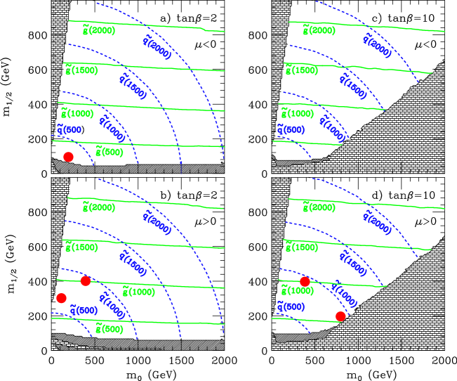
Figure 14: Gluino and squark masses^? in the minimal SUGRA model in the $m_{0}$-$m_{1/2}$ plane for $\tan\beta=2,10$, $\mathop{\rm sgn}\mu=\pm 1$, and $A_{0}=0$. The “bricked” regions are excluded theoretically, while the cross-hatched regions are excluded by experiment. The dots correspond to the five LHC points described in the text.

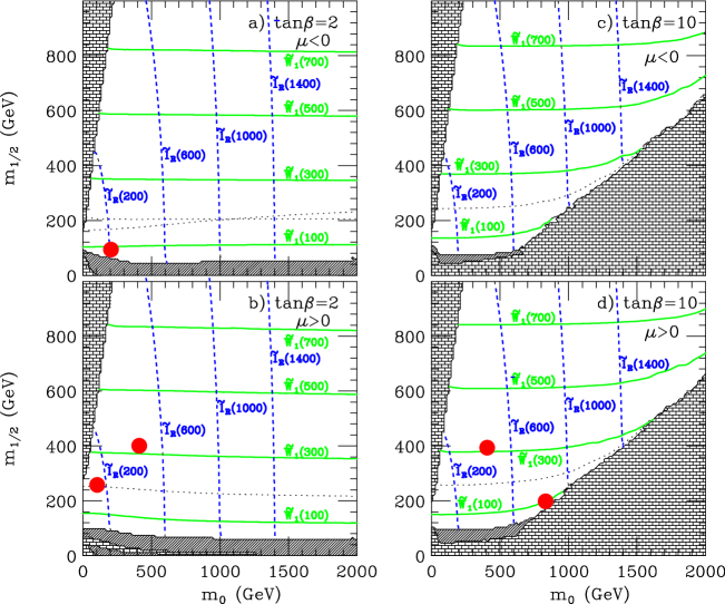
Figure 15: Gaugino and slepton masses^? in the minimal SUGRA model in the $m_{0}$-$m_{1/2}$ plane for $\tan\beta=2,10$, $\mathop{\rm sgn}\mu=\pm 1$, and $A_{0}=0$. The “bricked” regions are excluded theoretically, while the cross-hatched regions are excluded by experiment. The dots correspond to the five LHC points described in the text.

The solution of the renormalization group equations for the SUGRA model is built into ISAJET.^? The numerical solution of these equations uses Runge-Kutta step-by-step integration so that the thresholds corresponding to the various SUSY masses can be included in a self-consistent way. First, a truncated set of equations is used to determine a first estimate of the GUT scale, defined as the scale at which $\alpha_{1}$ and $\alpha_{2}$ meet. The GUT boundary conditions are then imposed, and the full set of equations is run back to the weak scale, freezing out mass parameters at their own scales. The 1-loop Higgs effective potential, including the SUSY masses, is computed, and the parameters $B$ and $\mu^{2}$ are eliminated in favor of $M_{Z}^{2}$ and $\tan\beta$. Some optimization of the scale choice is made; this is equivalent to including some 2-loop contributions. The equations are then iterated until a self-consistent solution is found. Once the renormalization equations have been solved, the sfermion and gaugino mixing matrices are computed, and all the branching ratios for SUSY particles are computed. In earlier versions mixings in the ${\tilde{b}}$ and ${\tilde{\tau}}$ sectors were ignored, limiting the program to $\tan\beta\mathrel{\hbox to0.0pt{\raise 2.20013pt\hbox{$<$}\hss}{\lower 2.20013pt\hbox{$\sim$}}}10$; this restriction has recently been removed. The branching ratio calculations use the correct matrix elements, but at present phase space is used in the actual event generation for technical convenience. Thus, for example, as a squark mass is varied from just below to just above the gluino mass, the branching ratio behaves sensibly but the event structure changes discontinuously.

PYTHIA^? uses approximate formulas rather than solving the renormalization group equations, or it can take masses from an external calculation. It treats the branching ratios in a similar way.

Figures 14 and 15 show contour plots of various SUSY masses in the $m_{0}$–$m_{1/2}$ plane for $\tan\beta=2,10$, $\mathop{\rm sgn}\mu=\pm 1$, and $A_{0}=0$ from ISAJET 7.22.^? The cross-hatched regions are excluded by experiment. The bricked regions at small $m_{0}$ are excluded by the requirement that the ${\tilde{\chi}_{1}^{0}}$ rather than the ${\tilde{\tau}}_{1}$ be the lightest SUSY particle. The bricked regions small $m_{1/2}$ and $\tan\beta=10$ were excluded in ISAJET 7.22 by the absence of electroweak symmetry breaking. It turns out that the size of this excluded region is very sensitive to the scale at which the effective potential is minimized; changes in recent versions of ISAJET intended to make the results more stable for $\tan\beta\gg 10$ have significantly reduced this region.

Figures 14 and 15 illustrate a number of general features of the SUGRA mass spectrum:

• Gluino and gaugino mass depend mainly on $m_{1/2}$.

• Slepton masses depend mainly on $m_{0}$.

• Squark masses depend mainly on $\sqrt{m_{0}^{2}+4m_{1/2}^{2}}$.

• $M_{\tilde{q}}\mathrel{\hbox to0.0pt{\raise 2.20013pt\hbox{$>$}\hss}{\lower 2.20013pt\hbox{$\sim$}}}0.9M_{\tilde{g}}$.

• $M_{\tilde{\chi}_{1}^{0}}\approx 0.5M_{{\tilde{\chi}}_{2}^{0}}\approx 0.5M_{{\tilde{\chi}}_{1}^{\pm}}\sim 0.5\times 0.3M_{\tilde{g}}$.

The last point is more general than the SUGRA model. It means that there is a large energy release at each step in the cascade decays of SUSY particles. If all the SUSY particles were nearly degenerate, they would be much more difficult to detect.

5.2 Reach of SUSY Signatures

Recall that a ${\tilde{g}}$ or ${\tilde{q}}$ is produced at the LHC with $p_{T}\sim M$ and decays into jets, possible leptons, and a ${\tilde{\chi}_{1}^{0}}$, which is neutral and weakly interacting and so escapes the detector. Thus the most generic prediction of ($R$-parity conserving weak scale) SUSY is an excess of events with multiple jets plus missing energy compared with the Standard Model sources, i.e., $W$, $Z$, and heavy quark production and mismeasurement of QCD jet events. The first task is to determine whether such an excess exists.

The standard requirement for discovery of a new phenomenon is a significance of at least $5\sigma$. That is, the probability that the background fluctuates up to the observed signal should be less than the tail of a Gaussian distribution beyond $5\sigma$, i.e., $5.7\times 10^{-5}$. This may seem overly conservative but is essential because one always looks at many different distributions with different cuts, and one of them is likely to have an unlikely fluctuation. For large numbers of events, the $5\sigma$ requirement is equivalent to

$$S/\sqrt{B}>5$$

where $S$ and $B$ are the number of signal and background events respectively. For small numbers, Poisson probabilities should be used. Of course the $S/B$ ratio, or more properly the error on determining what the background should be, must also be considered. Ruling out the existence of a signal is less demanding, and limits are generally quoted for 90% or 95% confidence.

The approach^?,? for determining the LHC reach in the SUGRA parameter space is to scan the $m_{0}-m_{1/2}$ plane for selected values of the other parameters, generating a sample of SUSY events for each choice of parameters. These consist mainly of ${\tilde{g}}$ and ${\tilde{q}}$ production, but all processes are included. Since one event typically takes about $0.5\,{\rm s}$ on an HP-735, the feasible data samples correspond to $\sim 10\,{\rm fb}^{-1}$ for detailed studies but much less for such a scan. It is clearly not possible to generate a representative sample of the Standard Model total cross section. Instead, high-$p_{T}$ events which potentially can give large $\hbox to0.0pt{\hbox to7.95831pt{\hfil/\hfil}\hss}E_{T}$, namely

• $W+{\rm jets}$, $W\to\ell\nu,\tau\nu$

• $Z+{\rm jets}$, $Z\to\nu\bar{\nu},\tau\tau$.

• $t\bar{t}$.

• QCD jets, including $g\to b\bar{b},c\bar{c}$ branching and decay.

These samples are generated using several approximately equal intervals of $\log p_{T}$ for the primary hard scattering. The event generator of course produces not just the hard scattering but also parton showers, hadronization of the partons into jets, and beam jets. The studies described here generally have assumed low luminosity, ${\cal L}=10^{33}\,{\rm cm^{-2}s^{-1}}$, and have therefore neglected pileup from overlapping events.

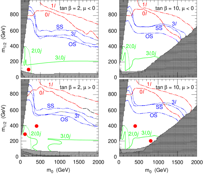
Figure 16: SUGRA reach in the $m_{0}$-$m_{1/2}$ plane for $\tan\beta=2,10$, $\mathop{\rm sgn}\mu=\pm 1$, and $A_{0}=0$ for $10\,{\rm fb}^{-1}$ luminosity at the LHC.^? The “bricked” regions are excluded theoretically, while the cross-hatched regions are excluded by experiment. The dots correspond to the points selected by the LHCC.

All events are passed through a toy detector simulation. This takes into account the overall coverage and Gaussian resolutions but not cracks, resolution tails, multiple scattering, or many other effects. It is possible to take all these effects into account, but the detector simulation then requires more than $1\,{\rm hr}$ per event. The toy simulation is not adequate to determine the $\hbox to0.0pt{\hbox to7.95831pt{\hfil/\hfil}\hss}E_{T}$ background from mismeasured QCD jets. More detailed studies show that this background is less than that from real Standard Model neutrinos for $\hbox to0.0pt{\hbox to7.95831pt{\hfil/\hfil}\hss}E_{T}\mathrel{\hbox to0.0pt{\raise 2.20013pt\hbox{$>$}\hss}{\lower 2.20013pt\hbox{$\sim$}}}100\,{\rm GeV}$, and this cut will generally be made whenever $\hbox to0.0pt{\hbox to7.95831pt{\hfil/\hfil}\hss}E_{T}$ is used.

Jets are found using a simple fixed-cone algorithm. That is, the highest remaining unused cell of the calorimeter is found, and the total $E_{T}$ is summed in a cone in

$$R=\sqrt{(\Delta\eta)^{2}+(\Delta\phi)^{2}}\,,$$

which is equivalent to a polar angle at $\eta=0$ but is $z$-boost invariant and so behaves properly in the forward direction. Generally $R=0.4$ is used for complex multijet events as a compromise between identifying nearby jets and containing all of the jet energy. Electrons and muons are treated equivalently, requiring isolation $E_{T}<5\,{\rm GeV}$ in cone $R=0.3$ both to suppress the $b,c\to\ell X$ background and to permit $e$ identification by track/shower matching. The latter requires a more detailed simulation to implement, so generator information is used for lepton identification.

Figure 16 summarizes the reach of the LHC to observe SUSY in various channels in the $m_{0}-m_{1/2}$ plane for two representative values of $\tan\beta$, $\mathop{\rm sgn}\mu=\pm 1$, and $A_{0}=0$. The reach limits are based on a $5\sigma$ signal after $10\,fb^{-1}$, corresponding to one year at low luminosity.

$0\ell$, $1\ell$: These curves show the reach in the basic channel, multiple jets plus missing energy. The $0\ell$ curve includes a veto on muons and isolated electrons, while the $1\ell$ curve requires a lepton. The lepton veto improves the $S/B$ ratio for low masses, but at high masses so many leptons are produced that requiring a lepton improves the reach. For both sets of curves the following cuts are made to reject the Standard Model background and to enhance the acceptance for heavy particles produced with $p_{T}\sim M$:

• $N_{\rm jets}\geq 2$ with $E_{T}>100\,{\rm GeV}$, $|\eta|<3$.

• Closest jet $j_{c}$ has $30^{\circ}<\Delta\phi(\hbox to0.0pt{\hbox to7.95831pt{\hfil/\hfil}\hss}E_{T},j_{c})<90^{\circ}$.

• $S_{T}>0.2$

• $\hbox to0.0pt{\hbox to7.95831pt{\hfil/\hfil}\hss}E_{T}>E_{T}^{c}$, $E_{T}(j_{1}),E_{T}(j_{2})>E_{T}^{c}$.

Here $E_{T}^{c}$ is a cut which is adjusted at each point to optimize $S/\sqrt{B}$, and the optimum value is used to define the reach. The variable $S_{T}$ is the transverse sphericity or circularity, which is defined as

$$S_{T}={2\lambda_{2}\over\lambda_{1}+\lambda_{2}}\,,$$

where $\lambda_{1}>\lambda_{2}$ are the eigenvalues of the transverse sphericity tensor

$$S_{ij}=\sum_{n}p_{n,i}p_{n,j}\,,\qquad i,j=1,2\,.$$

This cut selects “round” events characteristic of heavy particle production, but it is highly correlated with the multijet and other cuts.

$SS$: This curve shows the reach in the like-sign dilepton channel, $\ell^{\pm}\ell^{\pm}$, $\ell=e,\mu$. The leptons are required to have $p_{T}>20\,{\rm GeV}$ and $|\eta|<2.5$, and to satisfy the isolation criterion $E_{T}<5\,{\rm GeV}$ in a cone $R=0.3$. Since the gluino is a Majorana fermion, it is its own antiparticle and so has equal branching ratios into $\ell^{+}X$ and $\ell^{-}X$, e.g., through $\tilde{\chi}_{1}^{\pm}$ cascade decays. (There may be other SUSY sources of like-sign dileptons.) The dominant Standard Model isolated dilepton backgrounds, $t\bar{t}$, Drell-Yan, and $W^{+}W^{-}$, only give opposite-sign dileptons. There are Standard Model like-sign dilepton backgrounds, e.g., from $t\bar{t}$ production with $t\to\ell^{+}X$ and $\bar{t}\to\bar{b}\to\ell^{+}X$, but these will normally fail the isolation test.

$OS$: SUSY can also give opposite-sign dileptons $\ell^{+}\ell^{-}$, $\ell=e,\mu$. e.g., from ${\tilde{\chi}}_{2}^{0}\to{\tilde{\chi}_{1}^{0}}\ell^{+}\ell^{-}$. The same lepton cuts are made as for the $SS$ curves, and a $Z$ mass cut is also made for identical flavor leptons. Opposite-sign dilepton decays are enhanced at low $m_{0}$, for which the sleptons are light and the decay can proceed via ${\tilde{\chi}}_{2}^{0}\to{\tilde{\ell}}\ell\to{\tilde{\chi}_{1}^{0}}\ell^{+}\ell^{-}$ with substantial branching ratios. While the Standard Model backgrounds are larger in this channel than for $SS$, the statistical reach is comparable; the $OS$ channel also provides important independent information.

$3\ell$: SUSY can produce trilepton events from a variety of sources, including the decay of one gluino or squark via ${\tilde{\chi}}_{1}^{\pm}\to{\tilde{\chi}_{1}^{0}}\ell^{\pm}\nu$ and the other through ${\tilde{\chi}}_{2}^{0}\to{\tilde{\chi}_{1}^{0}}\ell^{+}\ell^{-}$. The Standard Model background for three isolated leptons is fairly small, so the reach in this channel is comparable to the dilepton channels even though the total branching ratio is smaller.

$3\ell,0j$, $2\ell,0j$: These channels require two or three leptons with the same cuts as before, $\hbox to0.0pt{\hbox to7.95831pt{\hfil/\hfil}\hss}E_{T}$, and no jets with $p_{T}>25\,{\rm GeV}$ and $|\eta|<3$. The jet veto is designed to select the direct production of gaugino or slepton pairs. These channels are the best way of searching for SUSY at the Tevatron, where the limited energy suppresses the production of the heavier gluinos and squarks. The search range is limited by competition from ${\tilde{\chi}}_{2}^{0}\to{\tilde{\chi}_{1}^{0}}Z,{\tilde{\chi}_{1}^{0}}h$ once $m_{1/2}$ is large enough that these are kinematically allowed.^? Even at smaller $m_{1/2}$ the branching ratio can be suppressed by interference between the virtual $Z$ and slepton exchange graphs, leading to the holes in the reach seen in Figure 16. Nevertheless, these channels would provide useful additional information should they be observed.

By comparing Figure 16 and the mass contours in Figure 14, one can see that the LHC can search the whole SUGRA parameter space at the $5\sigma$ level for gluino and squark masses up to about $2\,{\rm TeV}$ with only $10\,{\rm fb}^{-1}$ of luminosity. Similar conclusions have been found by the ATLAS^? and CMS^? Collaborations using the more general MSSM model and a more realistic parameterization of the detectors. In addition, various multilepton signatures can be observed for gluino and squark masses up to about $1\,{\rm TeV}$, i.e., over the whole range favored by fine-tuning arguments. The multilepton signatures with a jet veto are limited to relatively small values of $m_{1/2}$ or $m_{0}$. Thus, if SUSY exists at the weak scale, ATLAS and CMS should observe characteristic deviations from the Standard Model after one year of operation at only 10% of design luminosity. The LHC should either find SUSY or exclude it. Only experiment will decide whether SUSY at the weak scale is a crucial element in physics or an interesting exercise in mathematics.

5.3 Introduction to Precision Measurements

While observing signatures characteristic of SUSY at the LHC would be one of the most exciting developments in particle physics of all time, it is important to be able to determine the masses and other parameters of SUSY particles and thus to get a handle on the underlying dynamics. If $R$ parity is conserved, however, then every SUSY event is missing two ${\tilde{\chi}_{1}^{0}}$’s, and there are not enough kinematic constraints to determine their momenta.

It may be useful to compare the SUSY case with the production of $t\bar{t}$ at the Tevatron:

$$q+\bar{q}\to t+\bar{t}\to\ell^{+}\nu b+\bar{q}^{\prime}q^{\prime\prime}\bar{b}\,.$$

In these events there is one missing $\nu$ and hence three unknown kinematic variables $\vec{p}_{\nu}$. To determine these, there are two measured components of $\hbox to0.0pt{\hbox to7.95831pt{\hfil/\hfil}\hss}E_{T}$ and two additional constraints expressed as quadratic equations in the components of $\vec{p}_{\nu}$:

$$(p_{e}+p_{\nu})^{2} = M_{W}^{2}\,,$$

$$(p_{e}+p_{\nu}+p_{b})^{2} = (p_{q^{\prime}}+p_{q^{\prime\prime}}+p_{\bar{b}})^{2}\,.$$

Thus there is one more constraint than unknown; this is known in ancient bubble chamber terminology as a 1C fit. Using all the constraints, one can fully reconstruct the event despite the missing neutrino. If top were produced singly, then one would have only one quadratic constraint, a 0C fit; in this case $\vec{p}_{\nu}$ could still be reconstructed, but there would be a 2-fold ambiguity. Of course for $t\bar{t}$ production one can also reconstruct the 3-jet mass directly.

Table 3: Parameters for the five LHC SUGRA points.

Point	$m_{0}$	$m_{1/2}$	$A_{0}$	$\tan\beta$	$\mathop{\rm sgn}{\mu}$
	(GeV)	(GeV)	(GeV)
1	400	400	0	02.0	$+$
2	400	400	0	10.0	$+$
3	200	100	0	02.0	$-$
4	800	200	0	10.0	$+$
5	100	300	300	02.1	$+$

Table 4: Masses of the superpartners, in GeV, at the five LHC SUGRA points from ISAJET 7.22. The first and second generation squarks and sleptons are degenerate.

Point	1	2	3	4	5
$\widetilde{g}$	1004	1009	298	582	767
$\widetilde{\chi}_{1}^{\pm}$	325	321	96	147	232
$\widetilde{\chi}_{2}^{\pm}$	764	537	272	315	518
$\widetilde{\chi}_{1}^{0}$	168	168	45	80	122
$\widetilde{\chi}_{2}^{0}$	326	321	97	148	233
$\widetilde{\chi}_{3}^{0}$	750	519	257	290	497
$\widetilde{\chi}_{4}^{0}$	766	538	273	315	521
$\widetilde{u}_{L}$	957	963	317	918	687
$\widetilde{u}_{R}$	925	933	313	910	664
$\widetilde{d}_{L}$	959	966	323	921	690
$\widetilde{d}_{R}$	921	930	314	910	662
$\widetilde{t}_{1}$	643	710	264	594	489
$\widetilde{t}_{2}$	924	933	329	805	717
$\widetilde{b}_{1}$	854	871	278	774	633
$\widetilde{b}_{2}$	922	930	314	903	663
$\widetilde{e}_{L}$	490	491	216	814	239
$\widetilde{e}_{R}$	430	431	207	805	157
$\widetilde{\nu}_{e}$	486	485	207	810	230
$\widetilde{\tau}_{1}$	430	425	206	797	157
$\widetilde{\tau}_{2}$	490	491	216	811	239
$\widetilde{\nu}_{\tau}$	486	483	207	806	230
$h^{0}$	111	125	68	117	104
$H^{0}$	1046	737	379	858	638
$A^{0}$	1044	737	371	859	634
$H^{\pm}$	1046	741	378	862	638

For SUSY, there are two missing ${\tilde{\chi}_{1}^{0}}$’s and so six unknown momentum components in addition to the ${\tilde{\chi}_{1}^{0}}$ mass. The SUSY signal contains many different processes; there is no simple constraints like the $W$ mass in the top case, so there are only two constraints on the six variables from the two components of $\hbox to0.0pt{\hbox to7.95831pt{\hfil/\hfil}\hss}E_{T}$. Hence it is not possible to reconstruct the events in general. It is possible, however, to use the kinematic endpoints of various distributions to make a precise determination of combinations of masses. This is simplest in a $e^{+}e^{-}$ (or $\mu^{+}\mu^{-}$) collider, where the SUSY particles are produced with a known beam energy, giving extra constraints, but it is also possible at the LHC, as will be seen in Section 6 below.

While the possibility of making such precision measurements is quite general, which ones can be made depends on the assumed masses and branching ratios and so can be determined only by simulating in detail events for specific choices of the SUSY parameters. The LHC Committee (LHCC), the CERN committee overseeing the LHC experiments, selected the five SUGRA points listed in Table 3 for detailed study by the ATLAS and CMS collaborations. Point 3 is the “comparison point,” selected so that every existing or proposed accelerator could discover something. At this point, the Tevatron would discover winos and zinos, the LHC would discover gluinos and squarks, the NLC would discover sleptons, and LEP would have recently announced the discovery of a light Higgs boson with a mass of $68\,{\rm GeV}$. Points 1 and 2 have gluino and squark masses of about $1\,{\rm TeV}$ and so test the reach of the LHC for such masses. Point 4 has large $m_{0}$, so that sleptons and squarks are much heavier than gauginos and gluinos. It was also close to the boundary of the allowed electroweak symmetry breaking region with ISAJET 7.22, so that $\mu$ was quite small and there was large mixing between the gauginos and higgsinos. More recent versions of ISAJET find that Point 4 further from this boundary, so that $\mu$ is larger and the mixing of gauginos and higgsinos is smaller. Finally, Point 5 was chosen to be in the center of the region giving the right amount of cold dark matter for cosmology.^? Heavy stable ${\tilde{\chi}_{1}^{0}}$’s tend to overclose the universe; getting the right amount of cold dark matter generally requires enhancing the ${\tilde{\chi}_{1}^{0}}$ annihilation cross section and hence having relatively light sleptons.

The masses of the SUSY particles for these five points as calculated with ISAJET 7.22 are listed in Table 4. These masses and the corresponding branching ratios are used in all the analyses described below.

5.4 Effective Mass Analysis

The SUSY reach limits discussed in Section 5 are based on just counting the number of events with some specified set of cuts. Because QCD corrections to hadronic cross sections are large, the signal expected in the Standard Model is somewhat uncertain. It is therefore desirable to measure for some variable a distribution which agrees with the Standard Model in some range and then deviates from it, thus giving a more convincing signal and also providing an estimate of the SUSY mass scale.

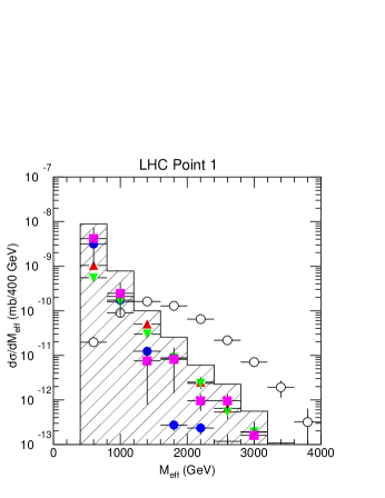
Figure 17: LHC Point 1 signal and Standard Model backgrounds.^? Open circles: SUSY signal. Solid circles: $t\bar{t}$. Triangles: $W\to\ell\nu$, $\tau\nu$. Downward triangles: $Z\to\nu\bar{\nu}$, $\tau\tau$. Squares: QCD jets. Histogram: sum of all backgrounds.

Figure 18: LHC Point 2 signal and Standard Model backgrounds.^? See Figure 17 for definitions of the symbols.

Figure 19: LHC Point 3 signal and Standard Model backgrounds.^? See Figure 17 for definitions of the symbols.

Figure 20: LHC Point 4 signal and Standard Model backgrounds.^? See Figure 17 for definitions of the symbols.

Figure 21: LHC Point 5 signal and Standard Model backgrounds.^? See Figure 17 for definitions of the symbols.

What properties should such a variable have? At least in the SUGRA model, the squarks are never much lighter than the gluino, so gluino production, which is enhanced by color and spin factors, is always important. If the squarks are heavier than the gluino, then the dominant gluino decays will be ${\tilde{g}}\to{\tilde{\chi}}q\bar{q}$, giving a minimum of four jets plus missing energy. If the gluino is heavier, then the decay chain ${\tilde{g}}\to{\tilde{q}}\bar{q}$, ${\tilde{q}}\to{\tilde{\chi}}q$ will dominate. In either case there will be at least four jets plus missing energy, more if one or more of the gauginos in the process decay hadronically. QCD cross sections fall rapidly with momentum transfer — the jet cross section at $\sqrt{s}=14\,{\rm TeV}$ falls over the relevant range of $p_{T}$ roughly like

$${d\sigma\over dp_{T}^{2}}\sim p_{T}^{-6}$$

— so it is clearly important to compare signal and background at comparable $p_{T}$ scales. The invariant mass of the produced system is not the best measure of this because it is too much influenced by possible soft jets at large rapidity. The scalar sum of the $p_{T}$’s of the four hardest jets and the $\hbox to0.0pt{\hbox to7.95831pt{\hfil/\hfil}\hss}E_{T}$ works well and will be called the “effective mass”^?

$$M_{\rm eff}=p_{T,1}+p_{T,2}+p_{T,3}+p_{T,4}+\hbox to0.0pt{\hbox to7.95831pt{\hfil/\hfil}\hss}E_{T}\,.$$

Backgrounds from QCD processes with multiple jets and neutrinos from heavy quarks generally have missing energy small compared to the $Q^{2}$ scale of the event. To avoid such backgrounds the $\hbox to0.0pt{\hbox to7.95831pt{\hfil/\hfil}\hss}E_{T}$ cut is made proportional to $M_{\rm eff}$,

$$\hbox to0.0pt{\hbox to7.95831pt{\hfil/\hfil}\hss}E_{T}>0.2M_{\rm eff}\,,$$

where the coefficient $0.2$ was chosen after studying the SUSY and Standard Model Monte Carlo distributions.

Table 5: The value of $M_{\rm eff}$ for which $S=B$ compared to $M_{\rm SUSY}$, the lighter of the gluino and squark ($\tilde{u_{R}}$) masses. Note that Point 3 is strongly influenced by the $\hbox to0.0pt{\hbox to7.95831pt{\hfil/\hfil}\hss}E_{T}$ and jet $p_{T}$ cuts.

LHC Point	$M_{\rm eff}\,({\rm GeV})$	$M_{\rm SUSY}\,({\rm GeV})$	Ratio
1	1360	926	1.47
2	1420	928	1.53
3	0470	300	1.58
4	0980	586	1.67
5	0980	663	1.48

Several additional cuts were made for technical reasons: a missing energy cut $\hbox to0.0pt{\hbox to7.95831pt{\hfil/\hfil}\hss}E_{T}>100\,{\rm GeV}$ to ensure that the Standard Model $\hbox to0.0pt{\hbox to7.95831pt{\hfil/\hfil}\hss}E_{T}$ background is dominated by neutrinos rather than mismeasured jets; a jet cut $p_{T,j}>50\,{\rm GeV}$ to ensure that the jets were well identified and measured, and a cut $p_{T,1}>100\,{\rm GeV}$ on the hardest jet to limit the range of QCD background that had to be generated. These cuts require $M_{\rm eff}>350\,{\rm GeV}$ and so limit the sensitivity to very light SUSY particles. In addition, there is a cut on transverse sphericity $S_{T}>0.2$ to select “round” events characteristic of SUSY, although this is highly correlated with the previous cuts. Finally, there is a veto on muons or isolated electrons with $p_{T}>15\,{\rm GeV}$; this minimizes the background for SUSY masses comparable to the top mass but reduces the sensitivity for high masses.

After all these cuts, the Standard Model background dominates the $M_{\rm eff}$ distribution for low $M_{\rm eff}$, but the SUSY signal dominates by a factor of 5–10 for large $M_{\rm eff}$ for all of the LHC points except the comparison point, Point 3, as can be seen from Figures 17–21. For Point 3, Figure 19, the SUSY signal is larger than the Standard Model background for all values of $M_{\rm eff}$ allowed by the technical cuts described above. Observing such a change in shape from a curve dominated by Standard Model physics to one a factor of 5–10 larger would be convincing evidence for new physics.

The signal curves in Figures 17–21 clearly shift with the SUSY masses. Since the SUSY cross section is dominated by ${\tilde{g}}$ and ${\tilde{q}}$ production, it is natural to use

$$M_{\rm SUSY}\equiv\min(M_{{\tilde{g}}},M_{\tilde{u}_{R}})$$

as a measure of the mass scale. Table 5 shows the points at which the signal and background points cross Figures 17–21. Clearly these points scale quite well with $M_{\rm SUSY}$.

Figure 22: Scatterplot of $M_{\rm SUSY}=\min(M_{{\tilde{g}}},M_{\tilde{u}})$ vs. $M_{\rm eff}$ for randomly chosen SUGRA models having the same light Higgs mass within $\pm 3\,{\rm GeV}$ as LHC Point 5.^?

Figure 23: Ratio $M_{\rm eff}/M_{\rm SUSY}$ from Figure 22.^?

To see whether the scaling in Table 5 might be accidental, a comparison of $M_{\rm eff}$ was made^? between 100 random SUGRA models and Point 5. The models were generated with parameters uniformly distributed in the intervals $100<m_{0}<500\,{\rm GeV}$, $100<m_{1/2}<500\,{\rm GeV}$, $-500<A_{0}<500\,{\rm GeV}$, $1.8<\tan\beta<12$, and $\mathop{\rm sgn}\mu=\pm 1$. All 100 models were selected to have $M_{h}$ within an assumed theoretical uncertainty of $\pm 3\,{\rm GeV}$ from the $M_{h}$ mass for Point 5. The value of $M_{\rm eff}$ for each model was determined not by the intersection with the Standard Model background but by the peak of the signal, which is somewhat higher. (It is not at all obvious that this is the optimal procedure, but it is what has been done.) The scatter plot of the peak $M_{\rm eff}$ vs. $M_{\rm SUSY}$ for each model is shown in Figure 22, and the projection is shown in Figure 23. Evidently the scaling of $M_{\rm eff}$ vs. $M_{\rm SUSY}$ works remarkably well for this random selection as well as for the five LHC points. While the scaling is physically plausible, it is not known how well it works for arbitrary SUSY models.

6 Precision Measurements with Exclusive Final States

While $M_{\rm eff}$ seems to work quite well as a measure of the SUSY mass scale, it clearly averages over many final states and branching ratios, so it can only be a rough approximation. To do better, one needs to reconstruct specific final states. If $R$ parity is conserved, then every SUSY event is missing two ${\tilde{\chi}_{1}^{0}}$’s, so no masses can be reconstructed directly. It is possible, however, to determine precisely combinations of masses by finding endpoints of kinematic distributions in specific final states, starting at the bottom of the decay chains for the SUSY particles and working up.^?,? For simple SUSY models such a SUGRA with only a few parameters, this approach can determine the model parameters with good accuracy, at least in favorable cases. Even for more complicated models it is a good starting point. This Section describes a number of such precision measurements^?,? for the five LHC SUGRA points.

6.1 Measurement of $M({\tilde{\chi}}_{2}^{0})-M({\tilde{\chi}_{1}^{0}})$

First consider Point 3. This point has unusual branching ratios because $M_{\tilde{b}}<M_{\tilde{g}}$ but $M_{\tilde{q}}>M_{\tilde{b}}$, so that ${\tilde{g}}\to{\tilde{b}}\bar{b}$ is very much enhanced:

$$B({\tilde{g}}\to{\tilde{b}}_{1}\bar{b}+{\rm h.c.}) =89\%\,,$$

$$B({\tilde{b}}_{1}\to{\tilde{\chi}}_{2}^{0}b) =86\%\,,$$

$$B({\tilde{\chi}}_{2}^{0}\to{\tilde{\chi}_{1}^{0}}\ell^{+}\ell^{-}) =33\%\,.$$

While these branching ratios are not typical, it is common for heavy flavors in SUSY decays to be comparable to light ones or even enhanced.

The SUSY particles at this point are relatively light and so give $\hbox to0.0pt{\hbox to7.95831pt{\hfil/\hfil}\hss}E_{T}$ in the range for which detector effects are not negligible. Hence, $\hbox to0.0pt{\hbox to7.95831pt{\hfil/\hfil}\hss}E_{T}$ is not used in the event selection at this point. Instead, events are selected by requiring

• $\ell^{+}\ell^{-}$ pair with $p_{T,\ell}>10\,{\rm GeV}$, $\eta<2.5$.

• $\geq 2$ jets tagged as $b$ quarks with $p_{T}>15\,{\rm GeV}$ and $\eta<2$.

• No $\hbox to0.0pt{\hbox to7.95831pt{\hfil/\hfil}\hss}E_{T}$ cut.

making use of the large ${\tilde{\chi}}_{2}^{0}\to{\tilde{\chi}_{1}^{0}}\ell^{+}\ell^{-}$ branching ratio. The details of the selection are certainly specific to this point, but it should be possible in general to use leptonic modes to observe SUSY particles in this low mass range.

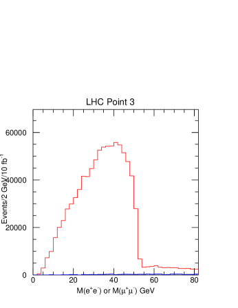
Figure 24: $\ell^{+}\ell^{-}$ mass for Point 3 (solid) and Standard Model background (shaded, nearly invisible).^?

SUSY signal and Standard Model background events were simulated as described above, and events were selected with the criteria just listed. Then the $\ell^{+}\ell^{-}$ mass distribution was plotted, including a 60% tagging efficiency for $b$’s and a 90% efficiency for electrons and muons. This mass distribution shows a spectacular edge at the $M({\tilde{\chi}}_{2}^{0})-M({\tilde{\chi}_{1}^{0}})$ endpoint, Figure 24. This distribution reflects the strong signal production, the large branching ratios, and the distinctive signature, resulting in almost no Standard Model background. The signal has huge statistics, and measuring the position of the edge is clearly easier than measuring the $W$ mass at the Tevatron, since only the lepton resolution and not the global $\hbox to0.0pt{\hbox to7.95831pt{\hfil/\hfil}\hss}E_{T}$ resolution enters. Since the latter has already achieved an error of about $40\,{\rm MeV}$, it seems conservative to estimate that one could measure the position of this edge and determine $M({\tilde{\chi}}_{2}^{0})-M({\tilde{\chi}_{1}^{0}})$ to $\sim 50\,{\rm MeV}$.

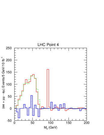
Figure 25: $M_{\ell^{+}\ell^{-}}$ distribution at Point 4 for opposite-sign, same-flavor dileptons (solid), opposite-sign, opposite-flavor dileptons (dashed) and Standard Model background (shaded).^?

The huge statistics from the low masses and the extra handle of the $b$ tag make this measurement unusually easy. But there is a similar edge at Point 4 plus a $Z$ peak coming from decays of the heavier gauginos. The dominant background is from two independent ${\tilde{\chi}}_{1}^{\pm}$ decays in SUSY events. This and the Standard Model backgrounds, e.g., from top decays, contribute equally to all combinations of leptons and so vanishes up to statistical fluctuations in the combination $e^{+}e^{-}+\mu^{+}\mu^{-}-e^{+}\mu^{-}-e^{-}\mu^{+}$. Figure 25 shows a plot of this difference for Point 4. The fluctuations in the background reflect the limited Monte Carlo statistics. Given the number of signal events, one could measure $\Delta\left(M({\tilde{\chi}}_{2}^{0})-M({\tilde{\chi}}_{1}^{0})\right)=\pm 1\,{\rm GeV}$ with $10\,{\rm fb}^{-1}$ at this point.

This method should work for any point for which the direct ${\tilde{\chi}}_{2}^{0}\to{\tilde{\chi}_{1}^{0}}\ell^{+}\ell^{-}$ branching ratio is not too small. This is generally the case for $M({\tilde{\chi}}_{2}^{0})\mathrel{\hbox to0.0pt{\raise 2.20013pt\hbox{$<$}\hss}{\lower 2.20013pt\hbox{$\sim$}}}200\,{\rm GeV}$ so that ${\tilde{\chi}}_{2}^{0}\not\to{\tilde{\chi}_{1}^{0}}Z$, ${\tilde{\chi}_{1}^{0}}h$. But there is a region of $m_{0}$ for $\mathop{\rm sgn}\mu=+1$ where the interference of the $Z$ and slepton exchange graphs makes the branching ratio small. This is the same effect that produces the holes in the $3\ell,0j$ reach curves in Figure 16.

6.2 Reconstruction of ${\tilde{g}}$ and ${\tilde{b}}_{1}$

The ${\tilde{\chi}}_{2}^{0}\to{\tilde{\chi}_{1}^{0}}\ell^{+}\ell^{-}$ decays at Point 3 can be combined with $b$ jets to reconstruct the ${\tilde{g}}\to{\tilde{b}}_{1}\bar{b}$, ${\tilde{b}}_{1}\to{\tilde{\chi}}_{2}^{0}b$ decay chain. The trick is to select an $\ell^{+}\ell^{-}$ pair near endpoint of the distribution. Then the ${\tilde{\chi}_{1}^{0}}$ must be soft in the $\ell^{+}\ell^{-}$ rest frame, so that

$$\vec{p}({\tilde{\chi}}_{2}^{0})\approx\left(1+{M({\tilde{\chi}_{1}^{0}})\over M(\ell\ell)}\right)\vec{p}(\ell\ell)\,,$$

where $M_{\tilde{\chi}_{1}^{0}}$ must be determined from the model. (A first approximation is $M({\tilde{\chi}}_{2}^{0})=2M({\tilde{\chi}_{1}^{0}})$, so that the $\ell^{+}\ell^{-}$ endpoint directly gives $M({\tilde{\chi}_{1}^{0}})$.) The following cuts are made for this analysis:

• $\geq 2$ jets tagged as $b$ jets with $p_{T}>15\,{\rm GeV}$, $\eta<2$;

• $\ell^{+}\ell^{-}$ pair with $45<M(\ell\ell)<55\,{\rm GeV}$.

Again, no use is made of $\hbox to0.0pt{\hbox to7.95831pt{\hfil/\hfil}\hss}E_{T}$. Then the inferred ${\tilde{\chi}}_{2}^{0}$ momentum is combined with one $b$ jet to make $M({\tilde{b}}_{1})$, and a second $b$ jet is added to make $M({\tilde{g}})$. A scatter plot including all the possible combinations for each event is shown in Figure 26. The projections of this scatter plot are shown in Figure 27.

Figure 26: Scatter plot of $M(b+{\tilde{\chi}}_{2})$ vs. $M(bb{\tilde{\chi}}_{2})-M(b{\tilde{\chi}}_{2})$ assuming $M_{\tilde{\chi}_{1}^{0}}$ known.^?

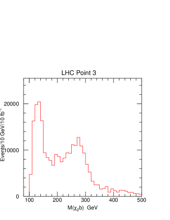
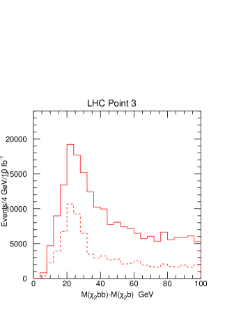
Figure 27: Projections of Figure 26.^? The dashed curve shows the mass difference for events in the ${\tilde{b}}$ mass peak.

Figure 26 was made assuming the correct ${\tilde{\chi}_{1}^{0}}$ mass, which is not directly measurable but must be determined from a global fit as described in Section 7 below. If $M({\tilde{\chi}_{1}^{0}})$ is varied about its nominal value, then the value of $M({\tilde{b}}_{1})$ extracted from Figure 27 shifts linearly, while the value of $M({\tilde{g}})-M({\tilde{b}}_{1})$ remains constant. Thus the errors on these masses are estimated to be

$$\Delta M({\tilde{b}}_{1})=\pm 1.5\Delta M({\tilde{\chi}_{1}^{0}})\pm 3\,{\rm GeV}\,,$$

$$\Delta(M({\tilde{g}})-M({\tilde{b}}_{1}))=\pm 2\,{\rm GeV}\,.$$

The fact that the difference $\Delta(M({\tilde{g}})-M({\tilde{b}}_{1}))$ is insensitive to the assumed mass is a simple consequence the kinematics and the fact that one $b$ jet is soft. Exactly the same effect is familiar from $D^{*}\to D\pi$ decays. In addition to the uncertainty from the ${\tilde{\chi}_{1}^{0}}$ mass, we must worry about the calibration of the hadronic energy scale. This can be studied using Standard Model events. For example, one could use $Z\to e^{+}e^{-}$ events to calibrate the electromagnetic calorimeter and then use $p_{T}$ balance in $\gamma+{\rm jets}$ and $Z+{\rm jets}$ events to transfer this calibration to the hadronic calorimeter. This is an important issue for the detector collaborations but need not concern us here.

6.3 Reconstruction of $h\to b\bar{b}$

For Point 5, the decay ${\tilde{\chi}}_{2}^{0}\to{\tilde{\chi}_{1}^{0}}h$ has a large branching ratio. A set of cuts similar to those made in the $M_{\rm eff}$ analysis is used to select the SUSY events and reject the Standard Model background:

• $\geq 4$ jets with $p_{T}>50\,{\rm GeV}$, $p_{T,1}>100\,{\rm GeV}$;

• Transverse sphericity $S_{T}>0.2$;

• $M_{\rm eff}>800\,{\rm GeV}$;

• $\hbox to0.0pt{\hbox to7.95831pt{\hfil/\hfil}\hss}E_{T}>\max(100\,{\rm GeV},0.2M_{\rm eff})$.

After these basic cuts, at least two jets are required to be tagged as $b$’s with the vertex detector and to have $p_{T,b}>25\,{\rm GeV}$ and $\eta_{b}<2$. The distribution of masses of all pairs of $b$ jets is shown in Figure 28. The width of the peak at the Higgs mass is set by clustering effects and resolution. The dominant background is other $b$ jets from SUSY events, not Standard Model background. This peak is much easier to detect than $h\to\gamma\gamma$ and would be the discovery mode of the Higgs boson at this point.

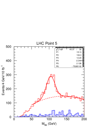
Figure 28: $M_{bb}$ distribution for Point 5 (solid), a Gaussian fit to the peak, and the Standard Model background (shaded).^?

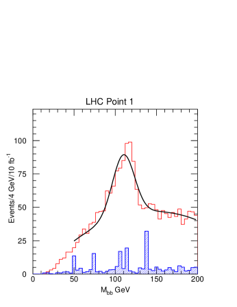
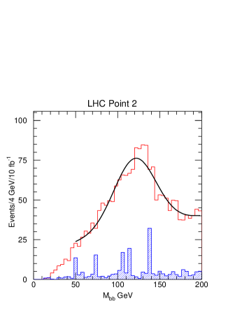
Figure 29: $M_{bb}$ distributions for Points 1 and 2.^? See Figure 28.

With the clustering algorithm described in Section 5.2 the Higgs peak actually came out several GeV below the Higgs mass. This is due partly to missing neutrinos and partly to leakage of energy out of the jet cone. A correction,

$$E_{b}^{\rm true}=1.08\left(E_{b}^{\rm observed}+2.9\,{\rm GeV}\right)\,,$$

was derived from the Monte Carlo data and applied to make Figure 28. In the real experiment, one would need to use the precision mass from $h\to\gamma\gamma$ to determine this correction.

The branching ratio for ${\tilde{\chi}}_{2}^{0}\to{\tilde{\chi}_{1}^{0}}h$ is generally substantial if it is kinematically allowed, i.e., for $m_{1/2}\mathrel{\hbox to0.0pt{\raise 2.20013pt\hbox{$>$}\hss}{\lower 2.20013pt\hbox{$\sim$}}}250\,{\rm GeV}$. There are similar Higgs mass peaks for the two other LHC points in this range; see Figure 29. One can hope to observe either ${\tilde{\chi}}_{2}^{0}\to{\tilde{\chi}_{1}^{0}}h$ or ${\tilde{\chi}}_{2}^{0}\to{\tilde{\chi}_{1}^{0}}\ell^{+}\ell^{-}$ over most of the parameter space.

It is also possible to reconstruct $W\to q\bar{q}$ at Point 5. Since there is no $b$ tag to select the relevant jets, the Standard Model backgrounds are large, and very hard cuts are needed.^?

6.4 Reconstruction of ${\tilde{g}}+{\tilde{g}}\to{\tilde{q}}_{L}q+{\tilde{q}}_{R}q$

Just as ${\tilde{\chi}}_{2}^{0}\to{\tilde{\chi}_{1}^{0}}\ell^{+}\ell^{-}$ was used as the starting point to reconstruct partially ${\tilde{b}}_{1}$ and ${\tilde{g}}$ at Point 3, one can use $h\to b\bar{b}$ as the starting point for more complex analyses. For example, at Point 5, the gluino is somewhat heavier than the squarks but has a larger cross section because of color and spin factors, producing as one possible signal

$${\tilde{g}}+{\tilde{g}}\to{\tilde{q}}_{L}q+{\tilde{q}}_{R}q\,,$$

$${\tilde{q}}_{L}\to{\tilde{\chi}}_{2}^{0}q\to{\tilde{\chi}_{1}^{0}}hq,\quad{\tilde{q}}_{R}\to{\tilde{\chi}_{1}^{0}}q\,.$$

The quark jets from the ${\tilde{q}}$ decays are hard, while the other jets are softer. These events can be selected by requiring in addition to the two $b$ jets two and only two additional jets with $p_{T}>75\,{\rm GeV}$. Then one of the two $qb\bar{b}$ combinations should come from a ${\tilde{q}}$ decay, so the smaller of the two $qb\bar{b}$ masses should have an endpoint at the kinematic limit for ${\tilde{q}}\to{\tilde{\chi}}_{2}^{0}q\to{\tilde{\chi}_{1}^{0}}hq$. This limit is readily found from two-body kinematics to be

$$(M_{hq}^{\rm max})^{2} = M_{h}^{2}+\left(M_{{\tilde{q}}}^{2}-M_{{\tilde{\chi}}_{2}^{0}}^{2}\right)$$

$$\times\left[{M_{{\tilde{\chi}}_{2}^{0}}^{2}+M_{h}^{2}-M_{{\tilde{\chi}_{1}^{0}}}^{2}+\sqrt{(M_{{\tilde{\chi}}_{2}^{0}}^{2}-M_{h}^{2}-M_{{\tilde{\chi}_{1}^{0}}}^{2})^{2}-4M_{h}^{2}M_{{\tilde{\chi}_{1}^{0}}}^{2}}}\over 2M_{{\tilde{\chi}}_{2}^{0}}^{2}\right]\,.$$

The average of the $u_{L}$ and $d_{L}$ masses gives $M_{hq}^{\rm max}=506\,{\rm GeV}$, which is consistent with the edge seen in Figure 30. The estimated error on this combination of masses is about one bin or $40\,{\rm GeV}$ for $10\,{\rm fb}^{-1}$. It is statistics limited and so should improve with more luminosity.

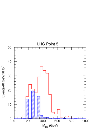
Figure 30: Smaller of two $b\bar{b}j$ masses at Point 5 (solid) and Standard Model background (shaded).^? The background statistics are limited by the Monte Carlo event sample.

6.5 $\ell^{+}\ell^{-}$ Distribution at Point 5

The $\ell^{+}\ell^{-}$ mass distribution has already been used to measure $M({\tilde{\chi}}_{2}^{0})-M({\tilde{\chi}_{1}^{0}})$ at Points 3 and 4. Consider now this mass distribution for Point 5, one of the points for which a ${\tilde{\chi}}_{2}^{0}\to{\tilde{\chi}_{1}^{0}}h$ signal has been observed. The event selection combines the same basic cuts as before plus the requirement of a lepton pair:

• $M_{\rm eff}>800\,{\rm GeV}$;

• $\hbox to0.0pt{\hbox to7.95831pt{\hfil/\hfil}\hss}E_{T}>0.2M_{\rm eff}$;

• $\geq 1$ jet with $p_{T}>100\,{\rm GeV}$;

• Isolated $\ell^{+}\ell^{-}$ pair with $p_{T}>10\,{\rm GeV}$, $\eta<2$;

• Transverse sphericity $S_{T}>0.2$.

The opposite-sign, same-flavor dilepton distribution after these cuts is shown in Figure 31 and obviously has a dramatic edge with very little background.

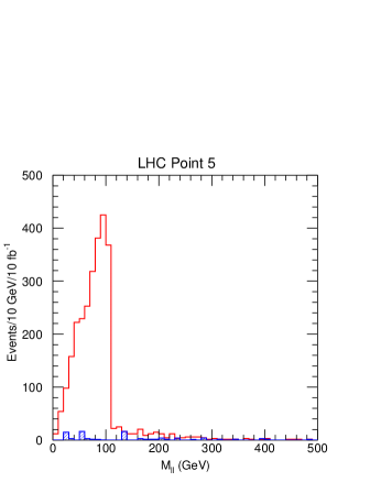
Figure 31: $M(\ell^{+}\ell^{-})$ distribution for Point 5 (solid) and Standard Model background (shaded).^?

It might at first seem that one should interpret this edge as a measure of $M({\tilde{\chi}}_{2}^{0})-M({\tilde{\chi}_{1}^{0}})$ from the kinematic limit of ${\tilde{\chi}}_{2}^{0}\to{\tilde{\chi}_{1}^{0}}\ell^{+}\ell^{-}$. But this interpretation is very implausible given the observation of $h\to b\bar{b}$ peak at this point, since this would require a 3-body decay to compete with a 2-body one, whereas 3-body phase space is much smaller than 2-body phase space. A much more plausible explanation is that another two-body decay, ${\tilde{\chi}}_{2}^{0}\to{\tilde{\ell}}\bar{\ell}$, gives rise to the dilepton endpoint. In SUGRA one generally has $M({\tilde{\ell}}_{R})<M({\tilde{\ell}}_{L})$, and in fact the observed endpoint in this case comes from

$${\tilde{\chi}}_{2}^{0}\to{\tilde{\ell}}^{\pm}\ell^{\mp}\to{\tilde{\chi}_{1}^{0}}\ell^{\pm}\ell^{\mp}\,.$$

Simple two-body kinematics for the ${\tilde{\chi}}_{2}^{0}\to{\tilde{\ell}}_{R}\bar{\ell}$ and ${\tilde{\ell}}_{R}\to{\tilde{\chi}_{1}^{0}}\ell$ decays gives for the $M(\ell^{+}\ell^{-})$ endpoint

$$M_{\rm max}(\ell\ell)=M({\tilde{\chi}}_{2}^{0})\sqrt{1-{M_{\tilde{\ell}}^{2}\over M_{\tilde{\chi}_{2}^{0}}^{2}}}\sqrt{1-{M_{{\tilde{\chi}_{1}^{0}}}^{2}\over M_{\tilde{\ell}}^{2}}}\,.$$

The estimated error on this combination of masses is about $1\,{\rm GeV}$ for $10\,{\rm fb}^{-1}$. It is statistics limited and so should improve with more luminosity.

This example illustrates that the interpretation of edges of kinematic distributions at the LHC may be ambiguous. If a signal for ${\tilde{\chi}}_{2}^{0}\to{\tilde{\chi}_{1}^{0}}h$, $h\to b\bar{b}$, had not already been observed at this point, it would not be clear whether the edge measured $M({\tilde{\chi}}_{2}^{0})-M({\tilde{\chi}_{1}^{0}})$ from direct decays or the above combination of three masses from decays through sleptons. Thus it is important to measure as many combinations of masses and distributions as possible so as to overconstrain models.

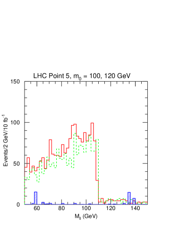
Figure 32: Same as Figure 31 but for Point 5 (solid) and $m_{0}=120\,{\rm GeV}$ (dashed), and Standard Model background (shaded).^?

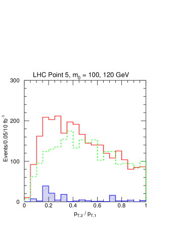
Figure 33: Ratio $p_{T}(\ell_{2})/p_{T}(\ell_{1})$ for Point 5 (solid), $m_{0}=120\,{\rm GeV}$ (dashed), and Standard Model background (shaded).^?

To get the maximum information from the dilepton distribution at this point, one should fit at least the $M(\ell\ell)$, $p_{T}(\ell\ell)$, $p_{T}(h)$, and $p_{T}(\ell_{2})/p_{T}(\ell_{1})$ distributions varying $M({\tilde{\chi}}_{2}^{0})$, $M(\tilde{\ell}_{R})$, $M({\tilde{\chi}_{1}^{0}})$, and the $p_{T}$ distribution of ${\tilde{\chi}}_{2}^{0}$. This is certainly what one would do if the distribution in Figure 31 were real experimental data, but it requires more effort than seems warranted now. Instead, one additional sample of events was generated with $m_{0}=120\,{\rm GeV}$ rather than $100\,{\rm GeV}$; this change increases $M(\ell_{R})$ by $13\,{\rm GeV}$ while having small effects on all the other relevant masses. As a result there is a $2\,{\rm GeV}$ change in the location of the edge, as seen in Figure 32. The changes in the $p_{T}$ distributions are small. The most significant change is in the distribution of the variable $p_{T}(\ell_{2})/p_{T}(\ell_{1})$, which is shown in Figure 33. This makes physical sense: increasing the slepton mass reduces the phase space and hence the $p_{T}$ for the first lepton, while increasing the phase space and the $p_{T}$ for the second lepton from the slepton. It is clear that a change of this magnitude is easily detected; the estimated error on the slepton mass from such measurement is $\sim 5\,{\rm GeV}$ on $m_{0}$ and $\sim 3\,{\rm GeV}$ on the slepton mass. Changing the slepton mass also changes the ${\tilde{\chi}}_{2}^{0}\to{\tilde{\ell}}\bar{\ell}$ branching ratio, providing additional information.

6.6 Measurement of $M({\tilde{g}})-M({\tilde{\chi}}_{2}^{0})$ and $M({\tilde{g}})-M({\tilde{\chi}}_{1}^{\pm})$ at Point 4

Gluino production dominates at Point 4 since $m_{0}\gg m_{1/2}$, so that the squarks are much heavier than the gluino. An analysis described previously for this point found a ${\tilde{\chi}}_{2}^{0}\to{\tilde{\chi}_{1}^{0}}\ell^{+}\ell^{-}$ edge and hence a measure of $M({\tilde{\chi}}_{2}^{0})-M({\tilde{\chi}_{1}^{0}})$. The jet multiplicity from gluino decay is large, so there is a lot of combinatorial background, and reconstructing a gluino signal is not trivial. The strategy for this analysis^? is to select

$${\tilde{g}}+{\tilde{g}}\to{\tilde{\chi}}_{2}^{0}q\bar{q}+{\tilde{\chi}}_{1}^{\pm}q\bar{q}$$

using leptonic decays of both gauginos to identify them and so to reduce the combinatorial background. Then the right combination of jet-jet masses has a common endpoint since $M({\tilde{\chi}}_{2}^{0})\approx M({\tilde{\chi}}_{1}^{\pm})$.

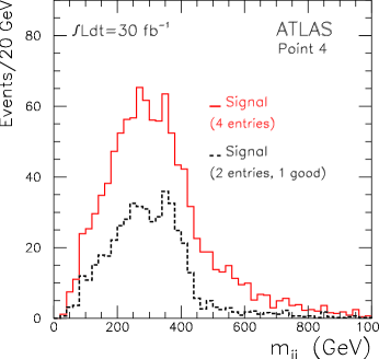
Figure 34: Jet-jet mass distribution for Point 4 with three leptons and four jets (solid) and for correct pairing (dashed).^?

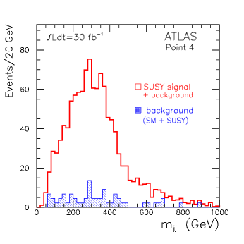
Figure 35: Jet-jet mass signal (solid) and background (shaded) for Point 4 with three leptons and four jets.^?

The event selection for this analysis imposes the following set of cuts:

• 3 isolated leptons with $p_{T}>20$, 10, $10\,{\rm GeV}$ and $|\eta|<2.5$, with one $OS$, $SF$ lepton pair.

• $M<72\,{\rm GeV}$, the edge in Figure 25, for the $OS$, $SF$ pair, consistent with ${\tilde{\chi}}20$ decay and not with possible $Z$ backgrounds.

• 4 jets with $p_{T}>150$, 120, 70, $40\,{\rm GeV}$ and $|\eta|<3.2$.

• No additional jets with $p_{T}>40\,{\rm GeV}$ and $|\eta|<5$ to minimize combinatorial backgrounds.

• No $\hbox to0.0pt{\hbox to7.95831pt{\hfil/\hfil}\hss}E_{T}$ cut.

After these cuts there 250 signal events with 30 ${\tilde{g}}{\tilde{q}}$ background and 18 other SUSY and Standard Model background for $30\,{\rm fb}^{-1}$ of integrated luminosity. Thus the signal purity is quite good, and the signal efficiency, $\sim 35\%$, is also good.

There are three ways of pairing the jets for event. The one that pairs the two highest and the two lowest $p_{T}$ jets is usually wrong since the ${\tilde{g}}$ are mainly at low $p_{T}$ and hence is removed.^? The distribution for the two remaining combinations, Figure 34, shows drop a near the endpoint for the correct combination of jets, shown as a dashed curve. The error on the mass was calculated by varying $M_{\tilde{g}}$, generating a new distribution, and using a Komogorov-Smirnov test to find whether the two distributions could be distinguished. The result of this analysis gives an estimated error

$$M_{\tilde{g}}-M_{{\tilde{\chi}}_{1}^{\pm}}/M{{\tilde{\chi}}_{2}^{0}}=434{+5.0\atop-16}\pm 4.5\,{\rm GeV}\,.$$

(The Komogorov-Smirnov test is a standard statistical test to see whether two distributions are identical. For a derivation and discussion, see Knuth.^?)

7 Global Fits to Determine SUSY Parameters

Section 6 has described a number of precision measurements that can be made at the LHC by relating features of kinematic distributions to combinations of SUSY masses. Quite a few other such measurements have been developed for these points, and many more would surely be found with the incentive of real data indicating the discovery of SUSY. It will also be possible to measure many other distributions that cannot be related to combinations of masses in such a precise way but which can be used to constrain the SUSY model. Given experimental observation of such signals, one would certainly use all the available data in a global fit to determine the SUSY model, just as the parameters of the Standard Model have been determined by global fits at LEP and SLC.

Making such a fit requires generating large samples of many possible SUSY signals, combining them with the Standard Model background, and comparing the results with the distributions for the assumed SUSY signal. This requires far more effort than can be justified at present. Instead, a much simpler approach has been adopted. Samples of signal events have been generated for each of the five LHC points. For each point, precision measurements of combinations of masses have been studied, and the errors on these combinations have been estimated. Then, SUGRA models have been generated choosing the parameters at random, the masses have been calculated, and the distributions of the model parameters have been determined for those models giving combinations of masses consistent with the precision measurements.

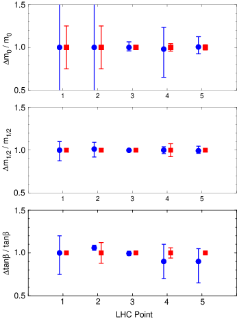
Figure 36: Errors on SUGRA parameters from the Hinchliffe et al.^? (circles) and Froidevaux^? (squares) fits.

Two such restricted global fits have been performed. The first fit is based on the set of precision measurements studied by Hinchliffe et al.^? and uses statistical errors appropriate to $10\,{\rm fb}^{-1}$, plus an assumed $3\,{\rm GeV}$ theoretical error on the light Higgs mass. The second fit, done by Froidevaux^? as part of the SUSY studies of the ATLAS Collaboration, is based on all of the Hinchliffe et al. measurements plus a number of additional ones and uses experimental errors scaled to three years at the full LHC design integrated luminosity, $300\,{\rm fb}^{-1}$. Froidevaux also assumes an error on the light Higgs mass set by the experimental error of $0.2\,{\rm GeV}$. That is, the Hinchliffe et al. fit is conservative both in regards to what is included and in regards to the integrated luminosity. The Froidevaux fit uses more distributions and the full LHC luminosity and it assumes a theoretical Higgs mass error much smaller than that currently available, so it requires a substantial improvement on the calculation of the Higgs effective potential in terms of the underlying SUGRA parameters. Nevertheless, even the results of Froidevaux might be improved by additional work and by studying actual data.

The results of these fits are shown in Figure 36, which displays the fractional errors for the Hinchliffe et al. and Froidevaux fits on each of the SUGRA parameters except $A_{0}$ at each of the five LHC points. Both fits do very well on $m_{1/2}$, the gaugino mass that sets the overall SUSY mass scale. The Hinchliffe, et al., fits do quite poorly on $m_{0}$ at Points 1 and 2 because the squark masses are insensitive to it and the slepton masses are too heavy to enter into any of the cascade decays. The Froidevaux fits do rather better because they include more information. The fits to $\tan\beta$ and $\mathop{\rm sgn}\mu$ uses $M_{h}$ heavily and so are sensitive to the assumed theoretical errors, which dominate over the experimental ones. Finally, neither fit gives a significant constraint on $A_{0}$. It is possible to constrain the weak-scale $A_{t}$, $A_{b}$, and $A_{\tau}$, but the renormalization group equations imply that these are only weakly related to $A_{0}$ and instead flow to quasi-fixed points.

Figure 36 shows that the LHC has the potential to determine the parameters of the SUSY model with good precision, at least for the cases studied. It is important to realize, however, that the use of a simple model is important in obtaining these results. Most of the measurements depend mainly on the gluino and squarks and on their main decay products, the lighter gauginos, ${\tilde{\chi}}_{1}^{0}$, ${\tilde{\chi}}_{2}^{0}$, or ${\tilde{\chi}}_{1}^{\pm}$, and the light Higgs boson $h$. It would be a useful exercise to vary the SUGRA model, e.g., by allowing splittings among the scalar masses, and to see how well these could be constrained.

8 Example Point with Large $\tan\beta$

When the five LHC points were selected, ISAJET and PYTHIA still neglected some mixing effects due to the $y_{b}$ and $y_{\tau}$ couplings. Hence it was necessary to choose points with $\tan\beta\leq 10$, for which these effects are small, since

$$\halign{\hbox to\displaywidth{$\hfil\displaystyle#\hfil$}\cr 0.0pt{\hfil$\displaystyle y_{t}={gm_{t}\over\sqrt{2}M_{W}\sin\beta}\,,\\ y_{b}={gm_{b}\over\sqrt{2}M_{W}\cos\beta}\,,\quad y_{\tau}={gm_{\tau}\over\sqrt{2}M_{W}\cos\beta}\,.\crcr}}$$

More recent versions of ISAJET have incorporated these mixing effects and so can be used for all values of $\tan\beta$. Large $\tan\beta$ has significant consequences for the phenomenology of the minimal SUGRA model:^?

• The renormalization group equations produce smaller ${\tilde{b}}_{L,R}$ and ${\tilde{\tau}}_{L,R}$ soft masses.

• The squark and slepton masses have larger off-diagonal terms, increasing the mixing and so reducing the ${\tilde{b}}_{1}$ and ${\tilde{\tau}}_{1}$ masses.

• The combination of smaller masses and larger Yukawa couplings enhance $b$ and $\tau$ decays.

• $M_{A}$ and related masses are also reduced.

Perhaps the most important consequence of these changes is that it is possible to have $M({\tilde{\tau}}_{1})<M({\tilde{\chi}}_{2}^{0}),M({\tilde{\chi}}_{1}^{\pm})$ but $M({\tilde{\ell}})>M({\tilde{\chi}}_{2}^{0}),M({\tilde{\chi}}_{1}^{\pm})$, leading to dominant $\tau$ decays of the gauginos.

“Point 6” is a minimal SUGRA point with $m_{0}=m_{1/2}=200\,{\rm GeV}$, $A_{0}=0$, $\tan\beta=45$, $\mu<0$. For this choice of $m_{0}$ and $m_{1/2}$, $W$, $Z$ and $h$ decays of the ${\tilde{\chi}}_{2}^{0}$ and ${\tilde{\chi}}_{1}^{\pm}$ are kinematically forbidden. Choosing $\tan\beta=45$ makes the ${\tilde{\tau}}_{1}$ light enough that $\tau$ decays of these gauginos are dominant, so that the ${\tilde{\chi}}_{2}^{0}\to{\tilde{\tau}}_{1}\bar{\tau}$ and ${\tilde{\chi}}^{\pm}\to{\tilde{\tau}}_{1}^{\pm}\nu_{\tau}$ decays are dominant, as can be seen from Figure 37.

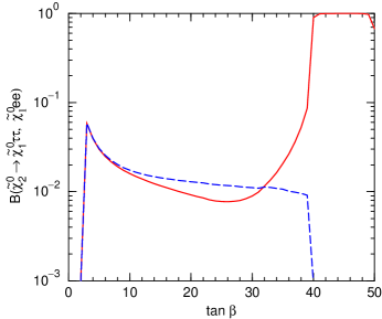
Figure 37: Branching ratios for ${\tilde{\chi}}_{2}^{0}\to{\tilde{\chi}_{1}^{0}}e^{+}e^{-}$ (dashed) and ${\tilde{\chi}_{1}^{0}}\tau^{+}\tau^{-}$ including ${\tilde{\tau}}_{1}^{\pm}\tau^{\mp}$ (solid).

The dominant decays of $\tau$’s are into leptons or into one or three charged hadrons:^?

$$\tau^{-}\to e^{-}\nu_{e}\nu_{\tau}\hfill \quad 17.8\%$$

$$\pi^{-}\nu_{\tau}\hfill \quad 11.3\%$$

$$\rho^{-}\nu_{\tau}\hfill \quad 25.2\%$$

$$a_{1}^{-}(1260)\hfill \quad 16.3\%\,.$$

The $a_{1}(1260)$ is an isovector, axial vector meson which dominantly decays into $\rho\pi$. Thus $\tau$’s can be identified experimentally as hadronic jets with a mass less than $M(\tau)=1.777\,{\rm GeV}$ and with either one charged track or three charged tracks with net charge $\pm 1$.

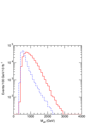
Figure 38: Effective mass $M_{\rm eff}$ for Point 6 signal (solid) and Standard Model background (dashed).

As is normally the case at the LHC, gluino and squark production dominate at this point. The same basic cuts are made as for the points discussed previously:

• $\geq 4$ jets with $p_{T,1}>100\,{\rm GeV}$, $p_{T,2,3,4}>50\,{\rm GeV}$.

• Missing energy $\hbox to0.0pt{\hbox to7.95831pt{\hfil/\hfil}\hss}E_{T}>100\,{\rm GeV}$.

• Transverse sphericity $S_{T}>0.2$.

• $M_{\rm eff}=\hbox to0.0pt{\hbox to7.95831pt{\hfil/\hfil}\hss}E_{T}+p_{T,1}+p_{T,2}+p_{T,3}+p_{T,4}>500\,{\rm GeV}$.

After these cuts, discovery is straightforward via multiple jets plus $\hbox to0.0pt{\hbox to7.95831pt{\hfil/\hfil}\hss}E_{T}$. Figure 38 shows the distribution of the variable $M_{\rm eff}$ defined previously for the signal and the sum of all Standard Model backgrounds. Evidently the signal dominates for large $M_{\rm eff}$ without using any $\tau$ identification cuts.

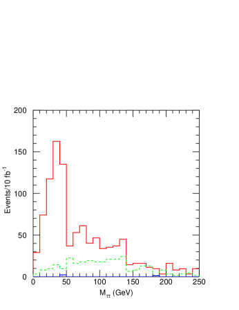
Figure 39: Visible $\tau^{+}\tau^{-}$ (solid) and $\tau^{\pm}\tau^{\pm}$ mass (dashed) for Point 6 and Standard Model background (shaded).

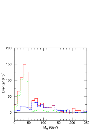
Figure 40: Visible $\tau^{+}\tau^{-}-\tau^{\pm}\tau^{\pm}$ mass for Point 6 signal (solid), ${\tilde{\chi}}_{2}^{0}$ decay contribution (dashed), and heavy gaugino contribution (dash-dotted).

After the above cuts, the signal is selected by requiring $M_{\rm eff}>500\,{\rm GeV}$, two hadronic $\tau$ decays, and no other isolated leptons. The $\tau$’s were selected using information from the event generator, since the actual detector cuts require rather a detailed analysis. Background from two independent decays, either from other SUSY channels or from Standard Model background, were removed by subtracting same-sign events from opposite-sign ones. Finally, only $\tau$ decays into three charged particles (mainly $a_{1}\nu_{\tau}$ and the $3\pi\nu_{\tau}$) were used. Since the 3-prong branching ratio is only about 15%, this involves a substantial loss in statistics, but the visible 3-prong momentum is closer to the true $\tau$ momentum. The opposite-sign and same-sign visible mass distributions after these cuts for the Point 6 signal and Standard Model background are shown in Figure 39. The difference of the opposite-sign and same-sign signals is shown in Figure 40. This figure also shows the contributions from ${\tilde{\chi}}_{2}^{0}\to{\tilde{\tau}}_{1}\bar{\tau}\to{\tilde{\chi}_{1}^{0}}\tau^{+}\tau^{-}$ and from events involving heavier gauginos. The former is responsible for the clear edge in the experimental distribution, while the latter dominates at larger masses.

Point 6 and similar points at which $\tau$ decays dominate will clearly be more difficult to study than points with decays into electrons and muons. More work is needed both to optimize the strategy and to understand the detector implications. Nevertheless, the results presented here are not unencouraging. Preliminary results indicate, however, that it will be difficult to detect any signals for such points at the Tevatron.

9 Higgs Bosons at LHC

Since the main reason for introducing SUSY at the weak scale is to cancel the quadratically divergent corrections to the Higgs masses, observing Higgs bosons at the LHC is just as important as observing SUSY particles. It is also a good deal more difficult, partly because the couplings to light quarks and hence the production cross sections are small, and partly because only some rare decay modes can be observed over the Standard Model backgrounds. Indeed, the ability to search for Higgs bosons has been the main design criterion for the detectors.^?,?

In the Minimal Supersymmetric Standard Model, there are five Higgs bosons,^? $h$, $H$, $A$, and $H^{\pm}$. These are described at tree level by just two parameters, generally taken to be the mass $M_{A}$ of the pseudoscalar Higgs boson and $\tan\beta$, the ratio of vacuum expectation values. The renormalization group equations and radiative electroweak symmetry breaking relate $M_{A}$ to the SUGRA parameters. The other masses are then given by

$$M_{H^{\pm}}^{2} = M_{A}^{2}+M_{W}^{2}$$

$$M_{h,H}^{2} = \frac{1}{2}\left[{M_{A}^{2}+M_{Z}^{2}\pm\sqrt{(M_{A}^{2}+M_{Z}^{2})^{2}-4M_{A}^{2}M_{Z}^{2}\cos^{2}2\beta}}\right]\,.$$

The mixing angle $\alpha$ between $h$ and $H$ is

$$\cos 2\alpha =-\cos 2\beta\left({\displaystyle{M_{A}^{2}-M_{Z}^{2}\over M_{H}^{2}-M_{h}^{2}}}\right)\,,$$

$$\sin 2\alpha =-\sin 2\beta\left({\displaystyle{M_{H}^{2}+M_{h}^{2}\over M_{H}^{2}-M_{h}^{2}}}\right)\,.$$

The couplings of the MSSM Higgs bosons relative to the Standard Model ones can all be expressed in terms of $\alpha$ and $\beta$, as shown in Table 6. Note that for $M_{A}\gg M_{Z}$, $\alpha\approx\beta-\frac{1}{2}\pi$, so that the light Higgs $h$ has couplings identical to those of a Standard Model Higgs of the same mass.

Table 6: MSSM Higgs couplings relative to a Standard Model Higgs of the same mass.

	$d\bar{d}$, $\ell^{+}\ell^{-}$	$u\bar{u}$	$WW$
$h$	$-\sin\alpha/\cos\beta$	$\cos\alpha/\sin\beta$	$\sin(\beta-\alpha)$
$H$	$\cos\alpha/\cos\beta$	$\sin\alpha/\sin\beta$	$\cos(\beta-\alpha)$
$A$	$-i\gamma_{5}\tan\beta$	$-i\gamma_{5}\cot\beta$	$0$

9.1 Observing Standard Model Higgs Bosons

The Standard Model Higgs is simpler than the MSSM Higgs sector and has been studied in more detail by ATLAS and CMS, so it makes sense to discuss it first. The dominant production is by $gg$ fusion through a $t$-quark loop, although $WW$ and $ZZ$ fusion also contribute for large masses. The same $5\sigma$ discovery limit discussed in Section 5.2 will be used here. The search for the Standard Model Higgs naturally divides into three mass regions^?,?:

$M_{H}>2M_{Z}$

The dominant Higgs decay modes in this mass region are $WW$ and $ZZ$, with $t\bar{t}$ at most $\sim 10\%$ and all other modes very small. The signal for $H\to ZZ\to\ell^{+}\ell^{-}\ell^{+}\ell^{-}$ is robust, with the only important background being the $ZZ$ continuum. It may also be possible to use the $H\to ZZ\to\ell^{+}\ell^{-}\nu\bar{\nu}$ and $H\to ZZ\to\ell^{+}\ell^{-}q\bar{q}$ modes, although the backgrounds in these channels are much more significant. The only problem in this region is that a very heavy Standard Model Higgs is strongly coupled to longitudinal $WW$ and $ZZ$ pairs, so that

$$\Gamma_{H}\approx{3G_{F}M_{H}^{3}\over 16\pi\sqrt{2}},\quad M_{H}\gg M_{Z}\,.$$

Thus at very large masses, $M_{H}>600$–$800\,{\rm GeV}$, the Higgs becomes so broad that it ceases to be a well defined particle and vanishes into the $WW$ or $ZZ$ continuum. Recent precision electroweak data from LEP indicates that the Standard Model Higgs is lighter than $420\,{\rm GeV}$ with 95% confidence.^? In this mass region, detection of a Higgs decaying into four leptons should be easy.

$130\,{\rm GeV}\mathrel{\hbox to0.0pt{\raise 2.20013pt\hbox{$<$}\hss}{\lower 2.20013pt\hbox{$\sim$}}}M_{H}<2M_{Z}$

In this mass region, the dominant Higgs decay mode is $H\to b\bar{b}$, but the background from QCD $b\bar{b}$ production is overwhelming. The best mode for detecting such a Higgs is $H\to ZZ^{*}\to\ell^{+}\ell^{-}\ell^{+}\ell^{-}$. While the rates are small, isolation cuts can be used to reject the $Zb\bar{b}$ background. Then, after the cuts $M_{12}\approx M_{Z}$ and $M_{34}>10\,{\rm GeV}$ to reject the $Z\gamma^{*}$ continuum, the $S/B$ is very good, as can be seen in Figure 41, although the signal is quite small. It seems clear that one can eventually detect a Higgs in this range, although it may take more than one year for $M_{H}\approx 170\,{\rm GeV}$, for which the $W^{+}W^{-}$ mode dominates.

Figure 41: Standard Model $H\to ZZ^{*}$ signals for $M_{H}=130$, 150, and $170\,{\rm GeV}$, showing both the average signal (top) and the signal for a typical experiment (bottom).^?

Table 7: $H\to ZZ^{*}$ event numbers.

Mass (GeV)	120	130	150	170	180
Signal ($3\times 10^{4}\,{\rm pb}^{-1}$)	2.6	12.5	34.9	10.2	26.5
$t\bar{t}$	$<0.1$	$<0.1$	$<0.1$	$<0.1$	$<0.1$
$Zb\bar{b}$	0.1	0.2	0.2	0.2	0.2
$ZZ^{*}$, $Z\gamma^{*}$	1.6	2.8	3.3	3.5	3.3
Background ($3\times 10^{4}\,{\rm pb}^{-1}$)	1.7	3.0	3.6	3.7	3.6
$S/\sqrt{B}$ ($3\times 10^{4}\,{\rm pb}^{-1}$)	2.0	7.2	18.3	5.3	14
Signal ($10^{5}\,{\rm pb}^{-1}$)	5.2	24.5	68.5	19.9	51.9
Background ($10^{5}\,{\rm pb}^{-1}$)	4.7	8.2	10.0	9.5	9.0
$S/\sqrt{B}$ ($10^{5}\,{\rm pb}^{-1}$)	2.4	8.5	21.7	6.5	17.3

For low statistics processes such as $H\to ZZ^{*}$, it is important to treat the statistics correctly. The right question to ask is, “What is the probability for the background to fluctuate up to the expected signal?” For large numbers of events, the answer is given by using Gaussian statistics to calculate the significance, $S/\sqrt{B}$, in standard deviations. For low numbers of events, however, it is important to use Poisson statistics and then to translate the probability to an equivalent Gaussian significance. Note, for example, that the Poisson probability for a background of 1 event to fluctuate up to 6 events is

$$P(5+1|1)={1^{6}e^{-1}\over 6!}=5.1\times 10^{-4}\,,$$

compared to $5\sigma$ Gaussian probability of $5.7\times 10^{-5}$. The probably that an expected signal $S+B=6$ fluctuates down to the background $B\leq 1$ is much larger:

$$P(0|6)+P(1|6)=e^{-6}[1+{6\over 1!}]=0.017\,.$$

Since there are many possible fake signals but presumably only one real one, this is acceptable.

The Gaussian significances shown in Table 7 are thus slightly too optimistic, but nevertheless they show that it is possible to discover a Higgs boson decaying through $ZZ^{*}$ into four leptons for $M_{H}\geq 130\,{\rm GeV}$. The maximum luminosity is needed for $M_{H}\sim 170\,{\rm GeV}$ because the $WW$ channel is open, reducing the $ZZ^{*}$ branching ratio. The acceptance used in this table may be somewhat optimistic, particularly for muons, but this can be compensated by more running time.

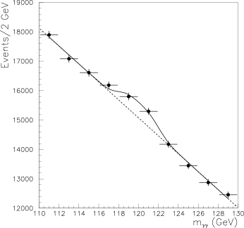
Figure 42: $120\,{\rm GeV}$ Standard Model Higgs signal and $\gamma\gamma$ background with the ATLAS detector.^?

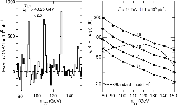
Figure 43: Background-subtracted signals for $H\to\gamma\gamma$ with the CMS detector and cross sections required for 5, 7, 10, and $15\sigma$ significance.^?

$M_{H}\mathrel{\hbox to0.0pt{\raise 2.20013pt\hbox{$<$}\hss}{\lower 2.20013pt\hbox{$\sim$}}}130\,{\rm GeV}$

Below about $130\,{\rm GeV}$ the $H\to ZZ^{*}\to\ell^{+}\ell^{-}\ell^{+}\ell^{-}$ branching ratio becomes too small to be observable, and the dominant $b\bar{b}$ and $\tau\tau$ modes are swamped by background. Thus in this mass range the only way to observe the Higgs is via the $\gamma\gamma$ mode. This mass region is particularly important for SUSY, since the light Higgs boson is always in this range and generally is almost identical to a Standard Model Higgs of the same mass. There are large backgrounds from the QCD $\gamma$-$\gamma$ continuum which can only be overcome with excellent $\gamma$-$\gamma$ mass resolution. There are also huge potential backgrounds from the $\gamma$-jet and jet-jet backgrounds. Detection of $H\to\gamma\gamma$ is an extraordinary challenge, and the need to do so has driven the design of the electromagnetic calorimeter — and, to a lesser extent, of the whole detector — for both ATLAS and CMS.

The first problem in detecting $H\to\gamma\gamma$ is to overcome the $\gamma\gamma$ continuum. The lowest order QCD process is $q\bar{q}\to\gamma\gamma$, but it is important to include the (gauge invariant) higher order process $gg\to\gamma\gamma$ through a box graph because $g(x)$ is very large at small $x$. The background calculation also includes $\gamma$ bremsstrahlung from quarks in the leading-log approximation. The following cuts are made in the ATLAS analysis to reduce this real $\gamma\gamma$ background compared to the signal:

• $p_{T,1}>40\,{\rm GeV}$, $p_{T,2}>25\,{\rm GeV}$, $|\eta|<2.5$.

• $p_{T,1}/(p_{T,1}+p_{T,2})<0.7$ to minimize bremsstrahlung backgrounds.

• Exclude regions of the calorimeter with degraded resolution.

• Choose $\Delta M$ for each mass to maximize $S/\sqrt{B}$.

With these cuts and with no fake $\gamma\gamma$ background, even the most favorable mass, $M_{H}=120\,{\rm GeV}$ is hard, as can be seen from Figure 42. Lower masses, $M_{H}<100\,{\rm GeV}$, are the most difficult, as can be seen from Figure 43. For a Standard Model Higgs in this mass range, one or more years at full luminosity are required to reach a $5\sigma$ significance. For all masses the $S/B$ ratio is poor, but because the peak is narrow, the side bands can be used to determine the background. Thus, the search limits are set by statistics and not by the understanding of the background.

The potential jet-jet and $\gamma$-jet backgrounds are very large; a $\gamma/{\rm jet}$ rejection of $\sim 10^{4}$ is essential to reduce these to a fraction of the QCD $\gamma\gamma$ continuum. Very detailed simulations of the isolation cuts and of the rejection of single and multiple $\pi^{0}$ using the detailed properties of the electromagnetic showers indicates that the required rejection can be achieved. An efficient trigger on two photons is also possible. But detecting this signal is probably the most difficult challenge for ATLAS and CMS.

Figure 44: Possible Higgs $5\sigma$ discovery contours for $30\,{\rm fb}^{-1}$ in various modes assuming all SUSY masses are $\sim 1\,{\rm TeV}$.^? Each signal is observable on the shaded side of the corresponding curve.

9.2 Observing SUSY Higgs Bosons

In the MSSM the Higgs sector at tree level depends only on two parameters, $M_{A}$ and $\tan\beta$. In the SUGRA model it is usually true that $M_{A}\gg M_{Z}$, so that the light Higgs $h$ is very similar to a Standard Model Higgs of the same mass, while the rest of the Higgs bosons are heavy, $M_{H}\approx M_{H^{\pm}}\approx M_{A}$. Many modes might be used to search for the SUSY Higgs bosons. Figures 44 and 45 show the $5\sigma$ reach contours^? for various signatures in the $M_{A}$-$\tan\beta$ plane, calculated assuming that all SUSY masses are $\sim 1\,{\rm TeV}$ so that SUSY decay modes do not contribute.^? Each mode has a statistical $5\sigma$ significance on the shaded side of the corresponding curve. The plot does not show constraints such as the rate for $b\to s\gamma$ that limit the Higgs parameter space for the assumed SUSY masses. Perhaps the only thing clear from these figures is that many modes can be used to search for SUSY Higgs bosons. By making use of all of the modes, it appears to be possible to discover at least one Higgs boson over the entire $M_{A}$–$\tan\beta$ plane by combining LEP at $195\,{\rm GeV}$ and ATLAS and CMS with $300\,{\rm fb}^{-1}$ each.^? Over much of the parameter space, more than one Higgs can be observed, but it is generally not possible to observe all of them.

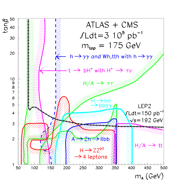
Figure 45: Possible Higgs $5\sigma$ discovery contours for $300\,{\rm fb}^{-1}$ in various modes assuming all SUSY masses are $\sim 1\,{\rm TeV}$.^? Each signal is observable on the shaded side of the corresponding curve.

All of the Standard Model Higgs search modes will be used to search for SUSY Higgs. In particular, in the SUGRA model the light Higgs $h$ is almost always in the range covered by the $\gamma\gamma$ mode because $M_{A}$ is large, so that the $h$ couplings are similar to the standard model ones. Hence the search for the $h$ is similar to that for a Standard Model Higgs in the same mass range. The $5\sigma$ discovery limits are indicated in Figures 44 and 45.

For the heavy Higgs bosons $H^{0}$ and $A^{0}$, the $ZZ$ modes are suppressed in the MSSM compared to the Standard Model. Because of $CP$ invariance, $A\not\to ZZ$, and the $H$ coupling to $WW$ and $ZZ$ is proportional to $\cos(\beta-\alpha)$, which vanished for large $M_{A}$. Hence the four-lepton modes are of limited value for SUSY Higgs, although there are regions indicated in Figures 44 and 45 where they can be observed.

Standard Model Higgs decays into $\tau\tau$ are probably not possible to observe. The $H$ and $A$ decays to $\tau\tau$ are enhanced for large $\tan\beta$, as can be seen from Table 6, and the competing $WW$ and $ZZ$ modes are reduced or eliminated. Since the $\tau$ always decays to a missing $\nu_{\tau}$, it is not possible to reconstruct the $\tau\tau$ mass in general. But if the Higgs is produced with high $p_{T}$, $p_{T}\mathrel{\hbox to0.0pt{\raise 2.20013pt\hbox{$>$}\hss}{\lower 2.20013pt\hbox{$\sim$}}}M_{H}$, then the two $\tau$’s are not back to back and it is possible to resolve the missing energy $\hbox to0.0pt{\hbox to7.95831pt{\hfil/\hfil}\hss}E_{T}$ along the observed $\tau$ directions, reconstructing the two $\tau$ momenta and hence the $\tau\tau$ mass. The mass resolution for such events has been studied with full simulation.^? The dominant $\tau\tau$ background is $Z^{*}/\gamma^{*}\to\tau\tau$, and this can be determined using $Z\to ee$, $\mu\mu$, and the known $\tau$ decay modes. Hence, the statistical errors should be dominant, and the $5\sigma$ discovery limits indicated in Figures 44 and 45 should be reliable.

The process $Wh\to\ell\nu b\bar{b}$ is another one that is difficult to observe for Standard Model Higgs, even though the lepton tag greatly reduces the Standard Model $b\bar{b}$ background. This signal is enhanced for large $\tan\beta$ in the MSSM and is at least statistically observable in the regions shown in Figures 44 and 45. But it must be noted that there is a large $t\bar{t}$ background: e.g., there are 475 signal events on 12700 background for a $100\,{\rm GeV}$ Standard Model Higgs. While this gives a statistical significance $S/\sqrt{B}=4.2$, it is necessary to know the background to better than 1% in order to be sure that the signal is real. While the $S/B$ for $H\to\gamma\gamma$ is also poor, the signal peak in that case is very narrow, so the sidebands can be used to determine the background. For $b\bar{b}$ decays the mass resolution will be of order 10%, and the $t\bar{t}$ background can produce background that varies significantly over this range. While it may be possible to observe this signal, the small value of $S/B$ implies that it will be very difficult.

10 Conclusions

If SUSY exists at the electroweak scale, i.e., with squark and gluino masses less than 1–$2\,{\rm TeV}$, it should be straightforward to find signals for it at the LHC in the ${\rm jets}+\hbox to0.0pt{\hbox to7.95831pt{\hfil/\hfil}\hss}E_{T}$ channel and perhaps in many other channels. Discovery of a deviation from the Standard Model should be possible with an integrated luminosity of $10\,{\rm fb}^{-1}$ or even less for masses below $1\,{\rm TeV}$. In many cases, it should be possible to determine combinations of masses from features of kinematic distributions, giving precision measurements of these mass combinations. If the SUSY model turns out to be simple, it will also be possible to determine its parameters from such precision measurements. Shortly after the LHC starts operation, either SUSY will become a central part of particle physics and of every subsequent TASI Summer School, or it will be relegated to an obscure corner of mathematical physics.

The LHC will mainly produce gluinos, squarks, and their main decay products, the light gauginos, ${\tilde{\chi}_{1}^{0}}$, ${\tilde{\chi}}_{2}^{0}$, and ${\tilde{\chi}}_{1}^{\pm}$. The dominant backgrounds for SUSY signatures come not from Standard Model processes but from other SUSY processes. For some choices of the SUSY model, it will also be possible to detect other SUSY particles, including some or all of the sleptons and the heavier gauginos. However, it is generally not possible to detect the whole SUSY and heavy Higgs spectrum. Thus, some of the conclusions from any LHC SUSY analysis will probably be model dependent.

The Next Linear Collider — or the Next Lepton Collider if a muon collider should turn out to be preferable — probably will be completed much later than the LHC. An NLC generally can detect all SUSY particles which are kinematically allowed. Using the fact that SUSY particles are pair produced at the beam energy allows one to reconstruct the ${\tilde{\chi}_{1}^{0}}$ mass as well as other masses.^?,? Such a machine may have to measure gauginos, Higgs’s, and perhaps sleptons with masses $\sim M_{\tilde{g}}$ This would require $\sqrt{s}>2M_{\tilde{g}}$. While this scale is not now known, it could be $2\,{\rm TeV}$. Of course, if the SUSY model turns out to be complicated, a lower energy machine capable of studying the sleptons and light gauginos could prove essential. There are exciting experimental prospects for SUSY not just at the LHC but at future machines.

I wish that I could be as optimistic about the future of particle physics in the United States.

It is a pleasure to thank my collaborators, including Howie Baer, Chih-Hao Chen, Manuel Drees, Daniel Froidevaux, Fabiola Gianotti, Ian Hinchliffe, Serban Protopopescu, Marjorie Shapiro, Jesper Söderqvist, Xerxes Tata, and Weiming Yao.

This work was supported in part by the United States Department of Energy under Contract DE-AC02-76CH00016.

References

References

- [1]
- [2] For general reviews of SUSY, see H.P. Nilles, Phys. Rep. 111, 1 (1984); H.E. Haber and G.L. Kane, Phys. Rep. 117, 75 (1985).
- [3] For a recent review of the MSSM, see S. Dawson, these proceedings.
- [4] P. Janot, Int. Euro. Conf. on High Energy Physics (Jerusalem, 1997), http://www.cern.ch/hep97/pl17.htm.
- [5] M. Carena, P. Zerwas, et al., hep-ph/9602250, CERN-96-01 (1996).
- [6] P.Q. Hung and M. Sher, Phys. Lett. B374, 138 (1996).
- [7] G.L. Kane, C. Kolda, and J.D. Wells, Phys. Rev. Lett. 70, 2686 (1993).
- [8] H. Baer, H. Murayama, X. Tata, et al., FSU-HEP-950401, hep-ph/9503479 (1995).
- [9] D0 Collaboration, Phys. Rev. Lett. 76, 2228 (1996).
- [10] H. Baer, C-H Chen, F.E. Paige, and X. Tata, Phys. Rev. D53, 6241 (1996).
- [11] L. Alvarez-Gaume, J. Polchinski and M.B. Wise, Nucl. Phys.B221, 495 (1983); L. Ibañez, Phys. Lett. 118B, 73 (1982); J.Ellis, D.V. Nanopolous and K. Tamvakis, Phys. Lett. 121B, 123 (1983); K. Inoue et al. Prog. Theor. Phys. 68, 927 (1982); A.H. Chamseddine, R. Arnowitt, and P. Nath, Phys. Rev. Lett., 49, 970 (1982).
- [12] ATLAS Collaboration, Technical Proposal, LHCC/P2 (1994).
- [13] CMS Collaboration, Technical Proposal, LHCC/P1 (1994).
- [14] LHC Management Board, http://wwwlhc01.cern.ch/planning.htm.
- [15] G.W. Anderson and D.J. Castano, Phys. Lett. B347, 300 (1995).
- [16] E. Eichten, I. Hinchliffe, K. Lane, and C. Quigg, Rev. Mod. Phys. 56, 579 (1984).
- [17] CTEQ Collaboration, Phys. Rev. D51, 4763 (1995).
- [18] T. Kinoshita, J. Math. Phys. 3, 650 (1962); T.D. Lee and M. Nauenberg, Phys. Rev. 140, B516 (1964).
- [19] For a very clear exposition, see S. Weinberg, Phys. Rev. 140, B516 (1965).
- [20] H.D. Politzer, Nucl. Phys. B129, 301 (1977).
- [21] J.C. Collins, D.E. Soper, and G. Sterman, in Perturbative QCD, ed. by A.H. Mueller (World Scientific, 1989, ISBN 9971505649), p. 1 and references therein.
- [22] G. Altarelli and G. Parisi, Nucl. Phys. B126, 298 (1977).
- [23] H. Baer, C-H Chen, F.E. Paige, and X. Tata, Phys. Rev. D52, 2746 (1995).
- [24] V.N. Gribov and L.N. Lipatov, Sov. J. Nucl. Phys. 15, 438 (1972).
- [25] Yu.L. Dokshitser, Sov. Phys. JETP 46, 641 (1978).
- [26] W. Beenakker, R. Hopker, M. Spira, and P.M. Zerwas, Nucl. Phys. B492, 51 (1997).
- [27] J. Kubar-Andre and F.E. Paige, Phys. Rev. D19, 221 (1979).
- [28] G. Altarelli, R.K. Ellis, and G. Martinelli, Nucl. Phys. B157, 461 (1979).
- [29] G. Marchesini, B.R. Webber, G. Abbiendi, I.G. Knowles, M.H. Seymour, and L. Stanco, hep-ph/9607393 (1996).
- [30] H. Baer, F.E. Paige, S.D. Protopopescu and X. Tata, in Physics at Current Accelerators and Supercolliders, ed. by J. Hewett, A. White and D. Zeppenfeld, (Argonne National Laboratory, 1993), hep-ph/9602203.
- [31] T. Sjostrand, LU-TP-95-20, hep-ph/9508391 (1995); S. Mrenna, Comput. Phys. Commun. 101, 232 (1997).
- [32] D. Knuth, Art of Computer Programming: Seminumerical Algorithms (Adisson Wesley, ISBN 0201038226).
- [33] For a recent review see B. Webber, hep-ph/9411384 (1994).
- [34] G.C. Fox and S. Wolfram, Nucl. Phys. B168, 285 (1980).
- [35] Particle Data Group, Phys. Rev. D54, 1 (1996).
- [36] A.H. Mueller and H. Navelet, Nucl. Phys. B282, 727 (1987).
- [37] CDF Collaboration, Phys. Rev. D41, 2330 (1990).
- [38] See, e.g., D.J. Castano, E.J. Piard, and P. Ramond, Phys. Rev. D49, 4882 (1994).
- [39] H. Baer, C.-H. Chen, and X. Tata, Phys. Rev. D55, 1466 (1997).
- [40] J. Bagger, hep-ph/9508392 (1995); pub. in Batavia Collider Workshop (1995).
- [41] J. Ellis and L. Roszkowski Phys. Lett. B283, 252, (1992); H. Baer and M. Brhlik, Phys. Rev. D53, 597 (1996).
- [42] I. Hinchliffe, F.E. Paige, M.D. Shapiro, J. Söderqvist, and W. Yao, Phys. Rev. D55, 5520 (1997).
- [43] A. Bartl, J. Söderqvist, et al., in Proc. 1996 Summer Study on High Energy Physics, ed. by D.G. Cassel and R.H. Siemann (Snowmass, 1996).
- [44] F. Gianotti, http://atlasinfo.cern.ch/Atlas/GROUPS/PHYSICS/- SUSY/susy.html (1996); ATLAS Phys-No-110 (1997).
- [45] H. Baer, C.-H. Chen, M. Drees, F.E. Paige, and X. Tata, Phys. Rev. Lett. 79, 986 (1997).
- [46] D. Froidevaux, http://atlasinfo.cern.ch/Atlas/GROUPS/PHYSICS/- SUSY/susy.html (1996).
- [47] J. Gunion, G. Kane, H. Haber, and S. Dawson, The Higgs Hunter’s Guide (Addison-Wesley, 1990, ISBN 0201509350).
- [48] E. Richter-Was, et al., ATLAS Note Phys-No-048 (1995).
- [49] D. Ward, Int. Euro. Conf. on High Energy Physics (Jerusalem, 1997), http://www.cern.ch/hep97/pl15.htm.
- [50] E. Richter-Was, et al., Phys-No-074 (1996).
- [51] T. Tsukamoto, K. Fujii, H. Murayama, M. Yamaguchi, and Y. Okada, Phys. Rev. D51, 3153, (1995).
- [52] M.M. Nojiri, K. Fujii, and T. Tsukamoto Phys. Rev. D54, 6756 (1996).